Manipulating P-and S-elastic waves in dielectric elastomers via external electric stimuli

Abstract

We investigate elastic wave propagation in finitely deformed dielectric elastomers in the presence of an electrostatic field. To analyze the propagation of both longitudinal (P-) and transverse (S-) waves, we utilize compressible material models. We derive explicit expressions of the generalized acoustic tensor and phase velocities of elastic waves for the ideal and enriched dielectric elastomer models. We analyze the slowness curves of the elastic wave propagation, and find the P-S-mode disentangling phenomenon. In particular, P- and S- waves are separated by the application of an electric field. The divergence angle between P- and S-waves strongly depends on the applied electrostatic excitation. The influence of the electric field is sensitive to material models. Thus, for ideal dielectric model the in-plane shear velocity increases with an increase in electric field, while for the enriched model the velocity may decreases depending on material constants. Similarly, the divergence angle gradually increases with an increase in electric field, while for the enriched model, the angle may be bounded. Material compressibility affects the P-wave velocity, and, for relatively compressible materials, the slowness curves evolve from circular to elliptical shapes manifesting in an increase of the reflection angle of P-waves. As a results, the divergence angle decreases with an increase in material compressibility.

1 Introduction

Dielectric elastomers (DEs) are soft responsive materials that can change their form and shape when subjected to electric stimuli [29, 3]. DEs have attracted considerable attention due to a large variety of possible applications ranging from artificial muscles and soft robotics to energy conversion and noise cancelling devises [28, 4, 6, 33, 21, 31, 25]. Figure 1 schematically illustrates a typical set-up of a planar DE actuator with deformation induced by applied voltage [49, 50, 16]. The DE layer coated with compliant electrodes contracts due to electrostatic attraction between oppositely charged electrodes.

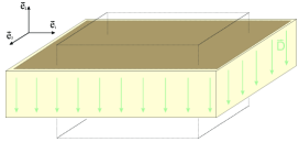
Figure 1: DE layer subjected to an electric field.

The theoretical framework of the non-linear electroelasticity is based on the theory first developed by Toupin [46, 47], which was recently revisited by Dorfmann and Ogden [9, 10] and Suo [44, 43]. This followed by a series of works on modeling DEs [45, 48, 18, 20, 8, 19, 24, 1], to name a few recent contributions. The electromechanical coupling in typical DEs is rather weak, and, therefore, DEs need to operate at the edge of instabilities and breakthrough voltages to achieve meaningful actuation [51, 30, 52, 53, 36, 34, 32, 14, 41]. Potentially, the need in the high voltage can be reduced through architectured microstructures of DEs and increasing the electromechanical coupling [17, 37, 5, 13], another promising approach is synthesis of new soft dielectric materials [23].

The effective electromechanical properties of DEs can be actively controlled by external electric stimuli. This opens an opportunity to manipulate wave propagation in DEs by applying electric field. In this work we focus on elastic wave propagation in finitely deformed DEs in the presence of an electric field. It is known that elastic wave propagation in purely elastic materials depends on the media mechanical properties and on the deformation [35, 12, 11]. In DEs the material moduli are modified by external electric field and induced deformations. To explore the elastic wave propagation in DEs, we follow the widely used approach of the analysis of small-amplitude motions superimposed on the finite deformations [27] induced by an external field [10]. To allow consideration of longitudinal wave propagation (as opposite to the recent works [15, 40, 7]), we utilize compressible electroactive material models, namely the ideal [51] and enriched DE models. By application of wave propagation analysis to the compressible DE models, we derive explicit expressions of generalized acoustic tensor and phase velocities for both longitudinal (P-) and transverse (S-) waves. We find that electrostatically induced changes in the important characteristics of shear and pressure waves lead to the disentangling phenomenon, where P- and S-waves travel in different directions. A schematic illustration of the P- and S-wave splitting phenomenon is shown in Fig. 2.

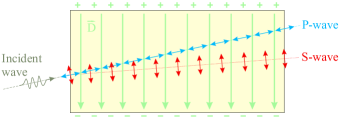
Figure 2: Schematics of the splitting of P-and S-elastic waves in a nearly incompressible neo-Hookean DE. P-wave does not refract from the initial direction of propagation, while S-wave refracts for a certain angle.

The divergence angle strongly depends on the external field, induced deformation, and material compressibility. P- and S-waves possess diverse properties and, thus, can be used for different purposes. For example, S-wave serves as a virtual ”finger” to probe the elasticity of the internal regions of the body in the shear wave elasticity imaging [39]. Longitudinal and transversal elastic waves can be separated on interfaces between dissimilar materials; however, in this case loss of energy or/and wave-mode conversion is encountered on the interface [2]. On this account we can use the phenomenon to split P-and S-elastic waves in dielectric elastomers by application of a bias electric field. This feature can be used, for example, in small-scale micro-electromechanical systems, where it is convenient to use electric field to control the performance.

2 Analysis

To analyse the finitely deformed state, we introduce the deformation gradient $\mathbf{F}(\vec{X},t)=\nabla_{\vec{X}}\otimes\vec{x}(\vec{X},t)$, where $\vec{X}$ and $\vec{x}$ are position vectors in the reference and current configurations, respectively. In order to model a non-linear electroelastic material behaviour, we consider an energy function $\psi(\mathbf{F},\vec{D}_{0})$ that is a function of the deformation gradient $\mathbf{F}$ and electric displacement vector $\vec{D}_{0}$ represented in the reference configuration. The corresponding electric displacement in the current configuration is given by $\vec{D}=J^{-1}\mathbf{F}\cdot\vec{D}_{0}$, where $J=\text{det}\leavevmode\nobreak\ \mathbf{F}$. Thus, the first Piola-Kirchhoff stress tensor and electric field in the reference configuration are given by

$$\mathbf{P}_{0}=\frac{\partial\psi}{\partial\mathbf{F}}\quad\text{and}\quad\vec{E}_{0}=\frac{\partial\psi}{\partial\vec{D}_{0}},$$ (1)

corresponding counterparts in the current configuration are

$$\mathbf{T}=J^{-1}\mathbf{P}_{0}\cdot\mathbf{F}^{T}\quad\text{and}\quad\vec{E}=\mathbf{F}^{-T}\cdot\vec{E}_{0}.$$ (2)

Next, we consider the small-amplitude motions superimposed on finite deformations. Incremental forms of the constitutive equations (1) are

$$\begin{split}\delta\mathbf{P}_{0}=\mathbb{C}_{0}:\delta\mathbf{F}+\mathcal{M}_{0}\cdot\delta\vec{D}_{0},\\ \delta\vec{E}_{0}=\delta\mathbf{F}:\mathcal{M}_{0}+\mathbf{K}_{0}\cdot\delta\vec{D}_{0},\end{split}$$ (3)

where $\delta$ denotes an increment change in a value on the right side; $\mathbb{C}_{0},\mathcal{M}_{0}$ and $\mathbf{K}_{0}$ are the so-called tensors of electroelastic moduli [10] defined as

$$\mathbb{C}_{0}=\frac{\partial^{2}\psi}{\partial\mathbf{F}\partial\mathbf{F}},\mathcal{M}_{0}=\frac{\partial^{2}\psi}{\partial\mathbf{F}\partial\vec{D}_{0}},\mathbf{K}_{0}=\frac{\partial^{2}\psi}{\partial\vec{D}_{0}\partial\vec{D}_{0}}.$$ (4)

Recall that $\mathbb{C}_{0}=\mathbb{C}_{0}^{(3412)}$ and $\mathbf{K}_{0}=\mathbf{K}_{0}^{T}$, where superscript (3412) denotes an isomer of the fourth-rank tensor [38, 26, 12] as detailed in A.

The incremental constitutive equations (3) in the frame of the updated reference configuration are

$$\delta\mathbf{P}=\mathbb{C}:\delta\mathbf{H}+\mathcal{M}\cdot\delta\vec{D}_{01},\delta\vec{E}_{01}=\delta\mathbf{H}:\mathcal{M}+\mathbf{K}\cdot\vec{D}_{01},$$ (5)

where $\delta\mathbf{P}=J^{-1}\delta\mathbf{P}_{0}\cdot\mathbf{F}^{T},\delta\vec{D}_{01}=J^{-1}\mathbf{F}\cdot\delta\vec{D}_{0},\delta\vec{E}_{01}=\mathbf{F}^{-T}\cdot\delta\vec{E}_{0},\delta\mathbf{H}=\delta\mathbf{F}\cdot\mathbf{F}^{-1}$ and

$$\begin{split}\mathbb{C}=&\ J^{-1}\left(\mathbf{F}\cdot\mathbb{C}_{0}^{(2134)}\cdot\mathbf{F}^{T}\right)^{(2134)},\\ \mathcal{M}=&\ \mathbf{F}\cdot\mathcal{M}_{0}^{(213)}\cdot\mathbf{F}^{-1},\\ \mathbf{K}=&\ J\mathbf{F}^{-T}\cdot\mathbf{K}_{0}\cdot\mathbf{F}^{-1}.\end{split}$$ (6)

Note that $\mathbb{C}=\mathbb{C}^{(3412)},\mathcal{M}^{(213)}=\mathcal{M}$ and $\mathbf{K}=\mathbf{K}^{T}$. The linearised equation of motion and Maxwell’s equations in Eulerian form are

$$\nabla_{\vec{x}}\cdot\delta\mathbf{P}=\rho\frac{\partial^{2}\vec{u}}{\partial t^{2}},\nabla_{\vec{x}}\times\delta\vec{E}_{01}=0,\nabla_{\vec{x}}\cdot\delta\vec{D}_{01}=0,$$ (7)

where $\vec{u}$ is incremental displacement and $\rho$ is material density. We seek for a solution of equations (7) in the form of plane waves with constant polarization

$$\vec{u}=\vec{m}f(\vec{n}\cdot\vec{x}-ct),\vec{D}_{01}=\vec{d}g(\vec{n}\cdot\vec{x}-ct),$$ (8)

where $f$ is a twice continuously differentiable function and $g$ is a continuously differentiable function; unit vectors $\vec{m}$ and $\vec{d}$ are polarization vectors of mechanical and electrical displacement, respectively; the unit vector $\vec{n}$ defines the direction of propagation of the wave, and $c$ is phase velocity of the wave.

By substitution (5) and (8) into (7), we obtain

$$\mathbf{A}\cdot\vec{m}=\rho c^{2}\vec{m},$$ (9)

where $\mathbf{A}$ is the so-called ”generalized” acoustic tensor which defines the condition of propagation of plane elastic waves in non-linear electroelastic materials. Moreover, for electroelastic materials with an arbitrary strain energy function $\psi(\mathbf{F},\vec{D}_{0})$ it has the following form [42]

$$\mathbf{A}=\mathbf{Q}-\frac{2}{(\text{tr}\hat{\mathbf{K}})^{2}-\text{tr}\hat{\mathbf{K}}^{2}}\mathbf{R}\cdot\left((\text{tr}\hat{\mathbf{K}})\hat{\mathbf{I}}-\hat{\mathbf{K}}\right)\cdot\mathbf{R}^{T},$$ (10)

where

$$\hat{\mathbf{I}}=\mathbf{I}-\vec{n}\otimes\vec{n}$$ (11)

is the projection on the plane normal to $\vec{n}$, $\hat{\mathbf{K}}=\hat{\mathbf{I}}\cdot\mathbf{K}\cdot\hat{\mathbf{I}}$ and

$$\mathbf{Q}=\mathbb{C}^{(1324)}:\vec{n}\otimes\vec{n},\mathbf{R}=\vec{n}\cdot\mathcal{M}.$$ (12)

It is worth mentioning that the generalized acoustic tensor $\mathbf{A}$ is symmetric as well as the purely elastic ”classic” acoustic tensor $\mathbf{Q}$. Recall that for DE to be stable, generalized acoustic tensor $\mathbf{A}$ has to be positively defined [42]. Detailed descriptions of the non-linear electroelastic theory for DEs can be found in works of Dorfmann and Ogden [9, 10], and Suo [44, 43].

It is well known that incompressible materials do not support longitudinal waves. Therefore, to analyse both transversal and longitudinal waves, we consider the energy function $\psi(\mathbf{F},\vec{D}_{0})$ for the compressible electroelastic material in the following form:

$$\psi(\mathbf{F},\vec{D}_{0})=\psi_{elas}(\mathbf{F})+\frac{1}{2\epsilon J}\left(\gamma_{0}I_{4e}+\gamma_{1}I_{5e}+\gamma_{2}I_{6e}\right),$$ (13)

where $\psi_{elas}(\mathbf{F})$ is the purely elastic energy function (for example, neo-Hookean, Mooney-Rivlin, Gent, etc. [27]), $\epsilon$ is the material permittivity in the undeformed state $\left(\mathbf{F}=\mathbf{I}\right)$ and $\gamma_{i}$ are dimensionless parameters, moreover $\gamma_{0}+\gamma_{1}+\gamma_{2}=1$, and

$$I_{4e}=\vec{D}_{0}\cdot\vec{D}_{0},I_{5e}=\vec{D}_{0}\cdot\mathbf{C}\cdot\vec{D}_{0},I_{6e}=\vec{D}_{0}\cdot\mathbf{C}^{2}\cdot\vec{D}_{0}$$ (14)

are invariants depending on the electric displacement $\vec{D}_{0}$ and right Cauchy-Green tensor $\mathbf{C}=\mathbf{F}^{T}\cdot\mathbf{F}$.

For energy function (13) the relation between the electric displacement and electric field is

$$\vec{E}=\frac{1}{\epsilon}\left(\gamma_{0}\mathbf{B}^{-1}+\gamma_{1}\mathbf{I}+\gamma_{2}\mathbf{B}\right)\cdot\vec{D},$$ (15)

where $\mathbf{B}=\mathbf{F}\cdot\mathbf{F}^{T}$ is the left Cauchy-Green tensor. The corresponding tensors of electroelastic moduli are

$$\begin{split}\mathbb{C}=&\mathbb{C}_{elas}+\frac{1}{2\epsilon}\left(\gamma_{0}\mathbb{C}_{4e}+\gamma_{1}\mathbb{C}_{5e}+\gamma_{2}\mathbb{C}_{6e}\right),\\ \mathcal{M}=&\frac{1}{2\epsilon}\left(\gamma_{0}\mathcal{M}_{4e}+\gamma_{1}\mathcal{M}_{5e}+\gamma_{2}\mathcal{M}_{6e}\right),\\ \mathbf{K}=&\frac{1}{\epsilon}\left(\gamma_{0}\mathbf{B}^{-1}+\gamma_{1}\mathbf{I}+\gamma_{2}\mathbf{B}\right),\end{split}$$ (16)

where $\mathbb{C}_{elas}$ is derived from the purely elastic part $\psi_{elas}(\mathbf{F})$ of the energy function in accordance to (4) and (6); and the explicit relations for the other tensors are given in the B.

Finally, the corresponding generalized acoustic tensor takes the following form

$$\mathbf{A}=\mathbf{Q}_{elas}+\frac{1}{2\epsilon}\left(\gamma_{0}\mathbf{Q}_{4e}+\gamma_{1}\mathbf{Q}_{5e}+\gamma_{2}\mathbf{Q}_{6e}-\frac{4}{\eta}\mathbf{A}_{e}\right),$$ (17)

where $\mathbf{Q}_{elas}$ is calculated by applying of Eq. (4), (6) and (12) to the purely elastic part $\psi_{elas}(\mathbf{F})$ of the energy function; the explicit expressions for $\eta$, and tensors $\mathbf{Q}_{4e}$, $\mathbf{Q}_{5e}$, $\mathbf{Q}_{6e}$ and $\mathbf{A}_{e}$ are given in the B. Remarkably, in the particular case of $\mathbf{F}=\lambda_{1}\vec{e}_{1}\otimes\vec{e}_{1}+\lambda_{2}\vec{e}_{2}\otimes\vec{e}_{2}+\lambda_{3}\vec{e}_{3}\otimes\vec{e}_{3}$, $\vec{n}=\vec{e}_{1}$ and $\vec{D}_{0}=D_{2}\vec{e}_{2}$ generalized acoustic tensor (17) reduces to

$$\mathbf{A}=\mathbf{Q}_{elas}+\frac{\gamma_{2}D_{2}^{2}}{\epsilon\lambda_{3}^{2}}\vec{e}_{2}\otimes\vec{e}_{2},$$ (18)

where ($\vec{e}_{1},\vec{e}_{2},\vec{e}_{3}$) is the orthonormal basis.

Let us consider how the application of an electric field affects the P-and S-wave propagation. Important characteristics of elastic waves can be deduced from consideration of slowness curves. Figure 3 schematically shows slowness curves for P-and S-waves for a nearly incompressible DE subjected to a voltage. Note that P-wave does not change its direction, while the S-wave refracts from initial direction. Thus, the P-and S-waves will be split when propagate in such media. It is easy to show that normal to slowness curves has the slope

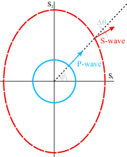
Figure 3: Slowness curves of pressure and shear waves in the nearly incompressible DE subjected to a voltage (for clarity, slowness curve of P-wave is zoomed in).

$$\text{tan}\leavevmode\nobreak\ \theta_{p,s}=\frac{s_{p,s}\leavevmode\nobreak\ \text{sin}\varphi-(ds_{p,s}/d\varphi)\leavevmode\nobreak\ \text{cos}\varphi}{s_{p,s}\leavevmode\nobreak\ \text{cos}\varphi+(ds_{p,s}/d\varphi)\leavevmode\nobreak\ \text{sin}\varphi},$$ (19)

where $\varphi$ is incident angle and $s_{p,s}=1/c_{p,s}$. Consequently, divergence angle between P-and S-wave can be calculated as $\Delta\theta=\theta_{p}-\theta_{s}$.

3 Results

3.1 Ideal dielectric elastomer model

First, we consider an ideal dielectric elastomer model [51], namely $\gamma_{0}=\gamma_{2}=0$ and $\gamma_{1}=1$ in (13). For an elastic part of the energy function (13), here and thereafter, we utilize a model of a compressible neo-Hookean material [27]

$$\psi_{elas}(\mathbf{F})=\frac{\mu}{2}(I_{1}-3)-\mu\ln\leavevmode\nobreak\ J+\left(\frac{K}{2}-\frac{\mu}{3}\right)(J-1)^{2},$$ (20)

where $I_{1}=\text{tr}\leavevmode\nobreak\ \mathbf{C}$ is the first invariant of the right Cauchy-Green tensor, $\mu$ is the shear modulus and $K$ is the bulk modulus.

For the ideal DE generalized acoustic tensor takes the form

$$\mathbf{A}=a_{1}^{*}\vec{n}\otimes\vec{n}+a_{2}^{*}\hat{\mathbf{I}},$$ (21)

where $\vec{n}\otimes\vec{n}$ is the projection on the direction $\vec{n}$ and $\hat{\mathbf{I}}$ is given in (11),

$$a_{1}^{*}=(K-2\mu/3)J+\mu J^{-1}(1+\vec{n}\cdot\mathbf{B}\cdot\vec{n})$$ (22)

$$\text{and}\quad a_{2}^{*}=\mu J^{-1}(\vec{n}\cdot\mathbf{B}\cdot\vec{n}).$$ (23)

Consequently, there always exist one pressure and two shear waves for any direction of propagation $\vec{n}$, finite deformation $\mathbf{F}$ and electric displacement $\vec{D}$. Phase velocities of these waves can be calculated as

$$c_{p}=\sqrt{a_{1}^{*}J/\rho_{0}}\quad\text{and}\quad c_{s}=\sqrt{a_{2}^{*}J/\rho_{0}},$$ (24)

where $\rho_{0}$ is the initial density of the material. Remarkably, while the electroelastic moduli (16) explicitly depend on electric field, phase velocities of elastic waves do not explicitly depend on the electric field. The dependence of the velocities on electric field is introduced through the electrostatically induced deformation. Specifically, dielectric elastomer coated with flexible electrodes contracts if a voltage is applied (see Fig. 1). Here we consider a case when electric field is orthogonal to the DE layer, i.e. $\vec{D}_{0}=D\sqrt{\mu\epsilon}\vec{e}_{2}$, and DE layer can freely expands in plane $\vec{e}_{1}-\vec{e}_{3}$ (Fig. 1). Thus, deformation gradient can be expressed as

$$\mathbf{F}=\lambda(D)\vec{e}_{2}\otimes\vec{e}_{2}+\tilde{\lambda}(D)(\mathbf{I}-\vec{e}_{2}\otimes\vec{e}_{2}).$$ (25)

For an incompressible ideal DE [51] $\lambda=(1+D^{2})^{-1/3}$ and $\tilde{\lambda}=\lambda^{-1/2}$. It should be noted that these relations approximately hold even for very compressible materials with $K/\mu\sim 1$ for a range of deformations and electric fields considered here. Recall that neo-Hookean DE is stable for $D\leqslant\sqrt{3}$ [51] and it will thin down without limit with further increase in electric field. Note that in the absence of an electric field, relations (24) reduce to $c_{p}=\sqrt{(K+4\mu/3)/\rho_{0}}$ and $c_{s}=\sqrt{\mu/\rho_{0}}$.

For the nearly incompressible DE, phase velocities of P- and S-waves can be calculated as

$$c_{p}=\sqrt{\left((K+\mu/3+\frac{\mu\left(1+D^{2}\text{cos}^{2}\leavevmode\nobreak\ \varphi\right)}{\left(1+D^{2}\right)^{2/3}}\right)/\rho_{0}}$$ (26)

and

$$c_{s}=\sqrt{\left(1+D^{2}\text{cos}^{2}\leavevmode\nobreak\ \varphi\right)\left(1+D^{2}\right)^{-2/3}\mu/\rho_{0}},$$ (27)

where the propagation direction is defined as $\vec{n}=(\text{cos}\varphi,\text{sin}\varphi,0)$. Hence, refraction angles of P-and S-waves are

$$\text{tan}\leavevmode\nobreak\ \theta_{p}=\frac{\left(K+\mu/3+\mu\left(1+D^{2}\right)^{-2/3}\right)\text{tan}\leavevmode\nobreak\ \varphi}{K+\mu/3+\mu\left(1+D^{2}\right)^{1/3}}$$ (28)

and

$$\text{tan}\leavevmode\nobreak\ \theta_{s}=\frac{\text{tan}\leavevmode\nobreak\ \varphi}{1+D^{2}}.$$ (29)

Remarkably, relations (26), (27),(28) and (29) approximately hold even for very compressible materials with $K/\mu\sim 1$ for a range of deformations and electric fields considered here.

Figure 4(a) shows that divergence angle $\Delta\theta$ significantly depends on the value of electric field. In particular, divergence angle monotonically increases with electric field until the limiting value of electric field is achieved ($D=\sqrt{3}$). Fig. 4(b) shows the dependence of the divergence angle $\Delta\theta$ on the incident angle $\varphi$. Clearly, the divergence angle $\Delta\theta$ has a maximum for a certain incident angle $\varphi_{0}$ depending on the applied electric field. The incident angle $\varphi_{0}$ corresponding to the maximal divergence angle is given by

$$\text{tan}\leavevmode\nobreak\ \varphi_{0}=\sqrt{\frac{\alpha\left(\alpha\mu^{3}\left(\alpha+27\right)+3D^{2}\alpha_{1}\mu\left(\alpha_{1}-3\mu\right)+\zeta\right)}{\mu^{3}\left(\alpha^{2}+27\right)+\zeta}},$$ (30)

where $\alpha=1+D^{2}$, $\alpha_{1}=\alpha^{2/3}\left(3K+\mu\right)$ and $\zeta=9K\alpha^{2}\left(\mu^{2}+3K\left(K+\mu\right)\right)$.

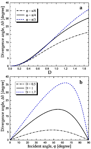
Figure 4: Divergence angle as functions of non-dimensional electric displacement – (a), and incident angle – (b) in the nearly incompressible neo-Hookean DE with $K/\mu=300$.

The angle $\varphi_{0}$ monotonically increases with increase in electric field. It is worth mentioning that for $\mu/K\ll 1$, $\varphi_{0}=\text{arccos}\left(2+D^{2}\right)^{-1/2}$.

Next we consider the influence of material compressibility on the elastic wave propagation in DEs. It was recently shown for purely mechanical materials that for highly compressible material phase velocity of longitudinal wave significantly depends on the direction of wave propagation and applied deformation [12]. Here, we also observe a strong dependence of P-wave velocity on the direction of wave propagation and deformation induced by an electric field. The more the material compressibility parameter $\mu/K$, the more the influence of electrostatically induced deformation on the elastic waves. In particular, slowness curves of P-wave evolve from circle to an ellipse shape with an increase in electric field. Thus, refraction angle of P-wave differs from the incident angle, namely P-wave refracts along with S-wave. The schematics of the phenomena is illustrated in Fig. 5.

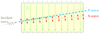
Figure 5: Schematics of the splitting of P- and S-waves in the compressible neo-Hookean DE. P-and S-wave unidirectionally refract from the initial direction of propagation, but the refraction angles are different.

It is clear that an increase in compressibility of the DE weakens the disentangling phenomenon. The dependence of the divergence angles as a function of compressibility for different values of applied electric field is presented in Fig. 6.

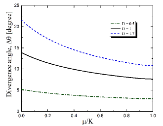
Figure 6: Divergence angle as functions of material compressibility for the ideal neo-Hookean DE, $\varphi=\pi/6$.

3.2 Enriched electroactive material model

Motivated by experimental data [50, 22], in this section we investigate elastic wave propagation in DEs described by an enriched electroactive material model (13). The model is similar to that considered by Gei et al [14]. To allow investigation of pressure waves, we extended the model to capture the compressibility effects. Table 1 summarizes the parameters of the material model (13) for different experimental data [50, 22].

Table 1: Material constants of DE model (13).

Reference	$\gamma_{0}$	$\gamma_{1}$	$\gamma_{2}$
Ideal DE [51]	0	1	0
Wissler and Mazza [50]	0.00104	1.14904	$-$0.15008
Li et al [22]	0.00458	1.3298	$-$0.33438

In case when $\gamma_{0}\not=0$, $\gamma_{2}\not=0$, deformation gradient is identical to (25), and $\vec{n}=\vec{e}_{1}$, phase velocities takes the following form

$$c_{p}^{(1)}=\sqrt{\left((K-2\mu/3)\lambda^{2}\tilde{\lambda}^{4}+\left(1+\tilde{\lambda}^{2}\right)\mu\right)/\rho_{0}},$$ (31)

$$c_{s}^{(2)}=\sqrt{\left(\gamma_{2}D^{2}\lambda+\tilde{\lambda}^{2}\right)\mu/\rho_{0}}$$ (32)

and

$$c_{s}^{(3)}=\tilde{\lambda}\sqrt{\mu/\rho_{0}}.$$ (33)

For incompressible materials $\tilde{\lambda}=\lambda^{-1/2}$, and $\lambda$ can be determined from the a solution of the following polynomial equation

$$\lambda^{3}\left(1+D^{2}\left(\gamma_{1}+2\gamma_{2}\lambda^{2}\right)\right)=1.$$ (34)

Hence, phase velocity of the shear wave with polarization $\vec{g}_{2}=\vec{e}_{2}$ (in-plane shear wave) explicitly depends on the electric field in contrast to the ideal DE. Figure 7 shows the phase velocity of the in-plane shear wave as a function of the non-dimensional electric field for the ideal DE and enriched DE models. One can see that consideration of the $I_{4e}$ and $I_{6e}$ invariants strongly affects the in-plane shear wave velocity. In particular, the increase in phase velocity of the in-plane shear wave is less prominent (dashed blue curve in Fig. 7) as compared to the ideal DE model result; moreover, the velocity may decrease with an increase in electric field for the particular material (dot-dashed green curve), while for the ideal DE model the velocity always increases.

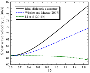
Figure 7: Phase velocity of in-plane shear wave as functions of non-dimentional electric displacement for $\varphi=0$.

These differences indeed affects the splitting mechanism and, thus, different results are produced by these material models. Figure 8 illustrates the difference in the divergence angels for the ideal DE and enriched DE models. In particular, Fig. 8(a) shows that divergence angle $\Delta\theta$ is smaller indeed than it was predicted by model of the ideal DE. Moreover, for Li et al. experimental data, divergence angle $\Delta\theta$ decreases with an increase in electric field when certain level of voltage is achieved. Fig. 8(b) shows that divergence angle $\Delta\theta$ has a maximum for a certain incident angle $\varphi_{1}$. Moreover, the incident angle $\varphi_{1}$, producing the maximum divergence angle, varies for different materials.

Although in this work we perform the fully electromechanical coupling analysis, it is possible to consider only purely mechanical analysis of wave propagation in non-linear electroelastic solid. Thus, contribution of the electroelastic moduli tensors $\mathcal{M}$ and $\mathbf{K}$ is neglected, and only terms of the tensor $\mathbb{C}$ contribute to the generalized acoustic tensor Remarkably, this approximation yields a very close results for the phase velocity of pressure wave, and exactly the same relations for the phase velocities of the shear waves. For example, for the deformation gradient (25), $\vec{n}=\vec{e}_{1}$ and $\vec{D}_{0}=D\sqrt{\mu\epsilon}\vec{e}_{2}$ classic acoustic tensor takes the form

$$\begin{split}\mathbf{Q}=&\ \mathbf{Q}_{elas}+\mu D^{2}(\gamma_{0}J^{-2}+\gamma_{1}\tilde{\lambda}^{-4}+\gamma_{2}\lambda^{2}\tilde{\lambda}^{-4})\vec{e}_{1}\otimes\vec{e}_{1}\\ &+\mu\gamma_{2}D^{2}\tilde{\lambda}^{-2}\vec{e}_{2}\otimes\vec{e}_{2}.\end{split}$$ (35)

It is easy to see that the resulting expressions for phase velocities of S-waves are the same as expressions (32) and (33), and expression for the phase velocity of P-wave has the form

$$\begin{split}c_{p}^{(1)}=&\ \sqrt{\mu/\rho_{0}}\Bigl{(}1+\tilde{\lambda}^{2}+(K/\mu-2/3)\lambda^{2}\tilde{\lambda}^{4}\\ &+D^{2}(\gamma_{0}\lambda^{-2}+\gamma_{1}+\gamma_{2}\lambda^{2})\tilde{\lambda}^{-4}\Bigr{)}^{-1/2}.\end{split}$$ (36)

Expression (36) for P-wave velocity differs from (31) in the additional term containing electric displacement magnitude. However, according to our observations for $K/\mu\gtrsim 100$, this term can be neglected for small and moderate levels of electric displacement.

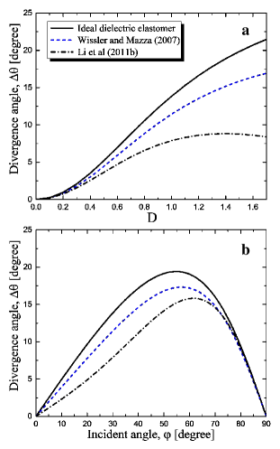
Figure 8: Divergence angle as functions of non-dimensional electric displacement for $\varphi=\pi/6$ (a) and incident angle for $D=1$ (b) in the nearly incompressible neo-Hookean DE with $K/\mu=300$.

4 Concluding remarks

In this paper, we considered P-and S-elastic waves in soft DEs subjected to an electric field. To allow consideration of P-wave propagation, we utilized the ideal and enriched material models containing compressibility effects. Explicit relations of the generalized acoustic tensor and phase velocities of elastic waves for the DE subjected to an electric field were presented. We found that, for the ideal DE elastic wave propagation is explicitly independent of the applied electric field, and it is influenced through deformation induced via bias electric field; this is despite the fact that all electroelastic moduli tensors explicitly depend on the applied electric field. However, for the enriched material model, including all three electroelastic invariants $I_{4e},I_{5e}$ and $I_{6e}$, elastic wave propagation explicitly depends on the applied electric field; namely, phase velocity of in-plane shear wave decreases when electric field is applied.

These findings were applied to explore the phenomenon of disentangling of P-and S-elastic waves in DEs by an electric field. We showed that divergence angle between P-and S-wave strongly depends on the value of the applied electric field and direction of wave propagation. Moreover, we found that an increase in the material compressibility weakens separation of P-and S-waves. This is due to the fact that P-wave also refracts along with the S-wave from the initial direction of wave propagation, while for nearly incompressible materials the change in its direction is negligible. The phenomenon can be used to manipulate elastic waves by a bias electrostatic field; this can be beneficial for an application at the small length-scale devices, such as micro-electromechanical systems, where electric field is a preferred control parameter.

Appendix A
Notation of a tensor isomer

Here we follow the notation of an isomer firstly introduced by Ryzhak [38, 26]. Let $\mathcal{S}$ be a third-rank tensor with the following representation as the sum of a certain number of triads:

$$\mathcal{S}=\mathbf{a}_{1}\otimes\mathbf{a}_{2}\otimes\mathbf{a}_{3}+\mathbf{b}_{1}\otimes\mathbf{b}_{2}\otimes\mathbf{b}_{3}+\ldots$$ (37)

Let (ijk) be some permutation of the numbers (123). Then the isomer $\mathcal{S}^{(ijk)}$ is defined to be the third-rank tensor determined by the relation

$$\mathcal{S}^{(ijk)}=\mathbf{a}_{i}\otimes\mathbf{a}_{j}\otimes\mathbf{a}_{k}+\mathbf{b}_{i}\otimes\mathbf{b}_{j}\otimes\mathbf{b}_{k}+\ldots$$ (38)

Analogously, we can define isomers for higher-rank tensors.

Appendix B
Components of the electroelastic moduli and generalized acoustic tensors

Here we introduce the following notations

$$\begin{split}L_{ab}=&\vec{a}\cdot\mathbf{L}\cdot\vec{b},L_{ab}^{(2)}=\vec{a}\cdot\mathbf{L}^{2}\cdot\vec{b},\mathbf{L}^{2}=\mathbf{L}\cdot\mathbf{L},\\ L_{ab}^{(-1)}=&\vec{a}\cdot\mathbf{L}^{-1}\cdot\vec{b},L_{ab}^{(-2)}=\vec{a}\cdot\mathbf{L}^{-2}\cdot\vec{b},\mathbf{L}^{-2}=\mathbf{L}^{-1}\cdot\mathbf{L}^{-1},\\ L_{ab}^{(3)}=&\vec{a}\cdot\mathbf{L}^{3}\cdot\vec{b},\mathbf{L}^{3}=\mathbf{L}^{2}\cdot\mathbf{L},L_{ab}^{(-3)}=\vec{a}\cdot\mathbf{L}^{-3}\cdot\vec{b},\\ \mathbf{L}^{-3}=&\mathbf{L}^{-2}\cdot\mathbf{L}^{-1},\vec{a}\otimes\vec{b}^{s}=\frac{1}{2}\left(\vec{a}\otimes\vec{b}+\vec{b}\otimes\vec{a}\right),\\ a_{b}=&\vec{a}\cdot\vec{b},a_{b}^{2}=(a_{b})^{2},\end{split}$$ (39)

where $\mathbf{L}$ is an arbitrary second-rank tensor; $\vec{a}$ and $\vec{b}$ are arbitrary vectors.

$$\begin{split}\mathbb{C}_{4e}=&\ B_{DD}^{-1}(\mathbf{I}\otimes\mathbf{I}+\mathbf{I}\otimes\mathbf{I}^{(1342)}),\\ \mathbb{C}_{5e}=&\ 2(\vec{D}\otimes\mathbf{I}\otimes\vec{D}^{(2134)}-\vec{D}\otimes\vec{D}\otimes\mathbf{I}-\mathbf{I}\otimes\vec{D}\otimes\vec{D})\\ &+D_{D}(\mathbf{I}\otimes\mathbf{I}+\mathbf{I}\otimes\mathbf{I}^{(1342)}),\\ \mathbb{C}_{6e}=&\ 2(\vec{D}\otimes\mathbf{I}\otimes(\mathbf{B}\cdot\vec{D})^{(2134)}+\mathbf{B}\otimes\vec{D}\otimes\vec{D}^{(1432)}\\ &+\vec{D}\otimes\mathbf{B}\otimes\vec{D}^{(2134)}+(\mathbf{B}\cdot\vec{D})\otimes\mathbf{I}\otimes\vec{D}^{(2134)}\\ &+\vec{D}\otimes\vec{D}\otimes\mathbf{B}^{(1324)}+\vec{D}\otimes\mathbf{B}\otimes\vec{D}\\ &-\mathbf{I}\otimes(\mathbf{B}\cdot\vec{D})\otimes\vec{D}-\mathbf{I}\otimes\vec{D}\otimes(\mathbf{B}\cdot\vec{D})\\ &-\vec{D}\otimes(\mathbf{B}\cdot\vec{D})\otimes\mathbf{I}-(\mathbf{B}\cdot\vec{D})\otimes\vec{D}\otimes\mathbf{I})\\ &+B_{DD}(\mathbf{I}\otimes\mathbf{I}+\mathbf{I}\otimes\mathbf{I}^{(1342)}).\end{split}$$ (40)

$$\begin{split}\mathbf{Q}_{4e}=&\ 2\ B_{DD}^{(-1)}\vec{n}\otimes\vec{n},\\ \mathbf{Q}_{5e}=&\ 2((D_{D}+D_{n}^{2})\vec{n}\otimes\vec{n}+D_{n}^{2}\hat{\mathbf{I}}-2D_{n}\vec{D}\otimes\vec{n}^{s})),\\ \mathbf{Q}_{6e}=&\ 2((2B_{Dn}D_{n}+B_{DD})\vec{n}\otimes\vec{n}+2B_{Dn}D_{n}\hat{\mathbf{I}}\\ &-2B_{Dn}\vec{D}\otimes\vec{n}^{s}+D_{n}^{2}\mathbf{B}+2D_{n}(\mathbf{B}\cdot\vec{n})\otimes\vec{D}^{s}\\ &-2D_{n}(\mathbf{B}\cdot\vec{D})\otimes\vec{n}^{s}+B_{nn}\vec{D}\otimes\vec{D}).\end{split}$$ (41)

$$\begin{split}\mathcal{M}_{4e}=&\ -2\mathbf{I}\otimes(\mathbf{B}^{-1}\cdot\vec{D}),\\ \mathcal{M}_{5e}=&\ 2(\vec{D}\otimes\mathbf{I}+\vec{D}\otimes\mathbf{I}^{(213)}-\mathbf{I}\otimes\vec{D}),\\ \mathcal{M}_{6e}=&\ 2(\vec{D}\otimes\mathbf{B}+\vec{D}\otimes\mathbf{B}^{(213)}+(\mathbf{B}\cdot\vec{D})\otimes\mathbf{I}\\ &+(\mathbf{B}\cdot\vec{D})\otimes\mathbf{I}^{(213)}-\mathbf{I}\otimes(\mathbf{B}\cdot\vec{D})).\end{split}$$ (42)

$$\begin{split}\mathbf{R}_{4e}=&\ -2\vec{n}\otimes(\mathbf{B}^{-1}\cdot\vec{D}),\\ \mathbf{R}_{5e}=&\ 2(D_{n}\mathbf{I}+\vec{D}\otimes\vec{n}-\vec{n}\otimes\vec{D}),\\ \mathbf{R}_{6e}=&\ 2(D_{n}\mathbf{B}+\vec{D}\otimes(\mathbf{B}\cdot\vec{n})+B_{Dn}\mathbf{I}\\ &+(\mathbf{B}\cdot\vec{D})\otimes\vec{n}-\vec{n}\otimes(\mathbf{B}\cdot\vec{D})).\end{split}$$ (43)

$$\begin{split}\eta=&\gamma_{0}^{2}\left(2B_{nn}^{(-2)}-\mathbf{B}^{-1}:\mathbf{B}^{-1}-(B_{nn}^{(-1)})^{2}\right)+\gamma_{2}^{2}\left(2B_{nn}^{(2)}-\mathbf{B}:\mathbf{B}-(B_{nn})^{2}\right)\\ &+\left(\gamma_{0}\left(\mathbf{I}:\mathbf{B}^{-1}-B_{nn}^{(-1)}\right)+\gamma_{1}\right)^{2}+\left(\gamma_{2}\beta+\gamma_{1}\right)^{2}+2\gamma_{0}\gamma_{2}\left((\mathbf{I}:\mathbf{B}^{-1})\beta-I_{1}B_{nn}^{(-1)}-1\right)\end{split}$$ (44)

$$\begin{split}\mathbf{A}_{e}=&\ a_{1}\vec{n}\otimes\vec{n}+a_{2}\mathbf{I}+a_{3}\vec{D}\otimes\vec{D}+a_{4}\vec{n}\otimes\vec{D}^{s}+a_{5}\mathbf{B}+a_{6}(\mathbf{B}\cdot\vec{n})\otimes\vec{D}^{s}\\ &+a_{7}(\mathbf{B}\cdot\vec{D})\otimes\vec{n}^{s}+a_{8}(\mathbf{B}\cdot\vec{n})\otimes\vec{n}^{s}+a_{9}\mathbf{B}^{2}+a_{10}(\mathbf{B}^{2}\cdot\vec{n})\otimes\vec{D}^{s}\\ &+a_{11}(\mathbf{B}^{2}\cdot\vec{D})\otimes\vec{n}^{s}+a_{12}(\mathbf{B}^{2}\cdot\vec{n})\otimes\vec{n}^{s}+a_{13}(\mathbf{B}\cdot\vec{n})\otimes(\mathbf{B}\cdot\vec{n})\\ &+a_{14}\mathbf{B}^{3}+a_{15}(\mathbf{B}^{3}\cdot\vec{n})\otimes\vec{D}^{s}+a_{16}(\mathbf{B}^{3}\cdot\vec{D})\otimes\vec{n}^{s}\\ &+a_{17}(\mathbf{B}^{2}\cdot\vec{n})\otimes(\mathbf{B}\cdot\vec{n})^{s}+a_{18}\mathbf{B}^{-1}+a_{19}(\mathbf{B}^{-1}\cdot\vec{n})\otimes\vec{n}^{s}\\ &+a_{20}(\mathbf{B}^{-1}\cdot\vec{n})\otimes\vec{D}^{s}+a_{21}(\mathbf{B}^{-1}\cdot\vec{D})\otimes\vec{n}^{s}\\ &+a_{22}(\mathbf{B}^{-1}\cdot\vec{n})\otimes(\mathbf{B}\cdot\vec{n})^{s}+a_{23}(\mathbf{B}^{-2}\cdot\vec{D})\otimes\vec{n}^{s},\end{split}$$ (45)

where

$$\begin{split}a_{1}=&\gamma_{0}^{3}\left(\left(B_{DD}^{(-2)}-(B_{Dn}^{(-1)})^{2}\right)\mathbf{I}:\mathbf{B}^{-1}-B_{nn}^{(-1)}B_{DD}^{(-2)}-B_{DD}^{(-3)}+2B_{Dn}^{(-1)}B_{Dn}^{(-2)}\right)+\gamma_{1}^{3}D_{D}\\ &+\gamma_{2}^{3}\left(\beta B_{DD}^{(2)}-B_{DD}^{(3)}\right)+2\gamma_{0}\gamma_{1}\gamma_{2}\left(\beta B_{DD}^{(-1)}+B_{Dn}B_{Dn}^{(-1)}+\beta_{4}B_{DD}-D_{D}\right)\\ &+\gamma_{0}\gamma_{1}^{2}\left(\beta_{4}D_{D}+B_{DD}^{(-1)}\right)+\gamma_{0}\gamma_{2}^{2}\left(\beta_{4}B_{DD}^{(2)}-3B_{DD}+2\beta D_{D}+2B_{Dn}^{(-1)}B_{Dn}^{(2)}\right)\\ &+\gamma_{1}\gamma_{0}^{2}\left(2\beta_{4}B_{DD}^{(-1)}-B_{DD}^{(-2)}+(B_{Dn}^{(-1)})^{2}\right)+\gamma_{1}\gamma_{2}^{2}\left(2\beta B_{DD}-B_{DD}^{(2)}\right)\\ &+\gamma_{2}\gamma_{0}^{2}\left(\beta B_{DD}^{(-2)}-3B_{DD}^{(-1)}+2\beta_{4}D_{D}+B_{Dn}^{(-1)}\left(2D_{n}-I_{1}B_{Dn}^{(-1)}\right)\right)+\gamma_{2}\gamma_{1}^{2}\left(\beta D_{D}+B_{DD}\right),\\ a_{2}=&\gamma_{1}^{3}D_{n}^{2}+\gamma_{2}^{3}\beta(B_{Dn})^{2}+2\gamma_{0}\gamma_{1}\gamma_{2}D_{n}\left(\beta_{4}B_{Dn}-D_{n}\right)+\gamma_{0}\gamma_{1}^{2}\beta_{4}D_{n}^{2}\\ &+\gamma_{0}\gamma_{2}^{2}\left(\beta_{4}B_{Dn}-2D_{n}\right)B_{Dn}+\gamma_{1}\gamma_{2}^{2}B_{Dn}\left(B_{Dn}+2\beta D_{n}\right)+\gamma_{2}\gamma_{1}^{2}\left(\beta D_{n}+2B_{Dn}\right)D_{n},\\ a_{3}=&\gamma_{2}^{2}\Bigr{(}\gamma_{2}\left(I_{1}\left(B_{nn}^{(2)}-(B_{nn})^{2}\right)+B_{nn}B_{nn}^{(2)}-B_{nn}^{(3)}\right)+\gamma_{0}\left(B_{nn}-B_{nn}^{(-1)}B_{nn}^{(2)}+(\mathbf{I}:\mathbf{B}^{-1})\left(B_{nn}^{(2)}-(B_{nn})^{2}\right)\right)\\ &+\gamma_{1}\left(B_{nn}^{(2)}-(B_{nn})^{2}\right)\Bigl{)},\\ a_{4}=&2\Bigr{(}\gamma_{0}\gamma_{1}\gamma_{2}\left(D_{n}-2\beta_{4}B_{Dn}\right)-\gamma_{1}^{3}D_{n}-\gamma_{2}^{3}\left(I_{1}B_{Dn}^{(2)}-B_{Dn}^{(3)}\right)-\gamma_{0}\gamma_{1}^{2}\beta_{4}D_{n}\\ &+\gamma_{0}\gamma_{2}^{2}\left(3B_{Dn}-\beta_{4}B_{Dn}^{(2)}+I_{1}\left(B_{Dn}^{(-1)}B_{nn}-2D_{n}\right)+D_{n}B_{nn}-B_{Dn}^{(-1)}B_{nn}^{(2)}\right)+\gamma_{1}\gamma_{2}^{2}B_{Dn}\left(B_{nn}-2I_{1}\right)\\ &+\gamma_{2}\gamma_{0}^{2}\left(B_{nn}\left(B_{Dn}^{(-1)}(\mathbf{I}:\mathbf{B}^{-1})-B_{Dn}^{(-2)}\right)-2D_{n}\beta_{4}\right)-\gamma_{2}\gamma_{1}^{2}\left(\beta D_{n}+2B_{Dn}\right)\Bigl{)},\\ a_{5}=&\gamma_{2}\Bigr{(}\gamma_{2}^{2}B_{Dn}\left(2D_{n}\beta-B_{Dn}\right)+2\gamma_{0}\gamma_{1}\beta_{4}D_{n}^{2}+\gamma_{0}\gamma_{2}D_{n}\left(2\beta_{4}B_{Dn}-D_{n}\right)\\ &+2\gamma_{1}\gamma_{2}\beta D_{n}^{2}+\gamma_{1}^{2}D_{n}^{2}\Bigl{)},\\ a_{6}=&2\gamma_{2}\Bigr{(}\gamma_{2}^{2}\left(D_{n}B_{nn}^{(2)}+I_{1}\left(B_{Dn}-D_{n}B_{nn}\right)\right)+\gamma_{0}\gamma_{1}\beta_{4}D_{n}+\gamma_{0}\gamma_{2}\left((\mathbf{I}:\mathbf{B}^{-1})\left(B_{Dn}-D_{n}B_{nn}\right)-B_{nn}^{(-1)}B_{Dn}\right)\\ &+\gamma_{1}\gamma_{2}\left(B_{Dn}+\beta D_{n}\right)+\gamma_{1}^{2}D_{n}\Bigl{)},\\ a_{7}=&-2\gamma_{2}\Bigr{(}\gamma_{2}^{2}\beta B_{Dn}+2\gamma_{0}\gamma_{1}\beta_{4}D_{n}+\gamma_{0}\gamma_{2}\left(\beta_{4}B_{Dn}-2D_{n}\right)+2\gamma_{1}\gamma_{2}\beta D_{n}+\gamma_{1}^{2}D_{n}\Bigl{)},\\ a_{8}=&2\gamma_{2}\Bigr{(}\gamma_{0}\gamma_{2}\left(B_{Dn}^{(-1)}\left(I_{1}D_{n}-B_{Dn}\right)-D_{n}^{2}\right)+D_{n}\Bigr{(}\gamma_{0}^{2}\left(B_{Dn}^{(-1)}(\mathbf{I}:\mathbf{B}^{-1})-B_{Dn}^{(-2)}\right)-\gamma_{2}^{2}B_{Dn}^{(2)}\\ &-\gamma_{0}\gamma_{1}B_{Dn}^{(-1)}-\gamma_{1}\gamma_{2}B_{Dn}\Bigl{)}\Bigl{)},\\ a_{9}=&\gamma_{2}^{2}D_{n}\left(\gamma_{2}\left(\beta D_{n}-2B_{Dn}\right)+D_{n}\left(\gamma_{0}\beta_{4}-\gamma_{1}\right)\right),a_{10}=2\gamma_{2}^{2}\left(\gamma_{2}\left(I_{1}D_{n}-B_{Dn}\right)+\gamma_{0}\beta_{4}D_{n}\right),\\ a_{11}=&2\gamma_{2}^{2}\left(\gamma_{2}\left(B_{Dn}-\beta D_{n}\right)-D_{n}\left(\gamma_{0}\beta_{4}-\gamma_{1}\right)\right),a_{12}=-2\gamma_{0}\gamma_{2}^{2}D_{n}B_{Dn}^{(-1)},\\ a_{13}=&\gamma_{2}^{2}D_{n}\left(\gamma_{2}\left(2B_{Dn}-I_{1}D_{n}\right)+\gamma_{1}D_{n}-\gamma_{0}D_{n}(\mathbf{I}:\mathbf{B}^{-1})\right),\\ a_{14}=&-\gamma_{2}^{3}D_{n}^{2},a_{15}=-2\gamma_{2}^{3}D_{n},a_{16}=-a_{15},a_{17}=-2a_{14},\\ a_{18}=&-\gamma_{0}\left(\gamma_{1}D_{n}+\gamma_{2}B_{Dn}\right)^{2},a_{19}=-2\gamma_{0}^{2}B_{Dn}^{(-1)}\left(\gamma_{1}D_{n}+\gamma_{2}B_{Dn}\right),\\ a_{20}=&2\gamma_{0}\gamma_{2}B_{nn}\left(\gamma_{1}D_{n}+\gamma_{2}B_{Dn}\right),\\ a_{21}=&2\gamma_{0}\left(\gamma_{2}\gamma_{0}\left(D_{n}-\beta_{4}B_{Dn}\right)-\gamma_{2}\beta\left(\gamma_{1}D_{n}+\gamma_{2}B_{Dn}\right)-\gamma_{1}\gamma_{0}\beta_{4}D_{n}\right),\\ a_{22}=&2\gamma_{0}\gamma_{2}D_{n}\left(\gamma_{1}D_{n}+\gamma_{2}B_{Dn}\right),a_{23}=2\gamma_{0}^{2}\left(\gamma_{1}D_{n}+\gamma_{2}B_{Dn}\right),\\ \beta=&I_{1}-B_{nn}\quad\text{and}\quad\beta_{4}=\mathbf{I}:\mathbf{B}^{-1}-B_{nn}^{(-1)}.\end{split}$$ (46)

References

References

- [1] J. Aboudi. Micro-electromechanics of soft dielectric matrix composites. International Journal of Solids and Structures, 64:30–41, 2015.
- [2] J. D. Achenbach. Wave Propagation in Elastic Solids. Applied Mathematics and Mechanics. North-Holland Publishing Company, 1973.
- [3] Y. Bar-Cohen. Electroactive polymers as artificial muscles: A review. Journal of Spacecraft and Rockets, 39(6):822–827, 2002.
- [4] P. Brochu and Q. Pei. Advances in dielectric elastomers for actuators and artificial muscles. Macromolecular Rapid Communications, 31(1):10–36, 2010.
- [5] C. Cao and X. Zhao. Tunable stiffness of electrorheological elastomers by designing mesostructures. Appl. Phys. Lett., 103(4), 2013.
- [6] F. Carpi, D. De Rossi, R. Kornbluh, R. Pelrine, and P. Sommer-Larsen. Dielectric Elastomers as Electromechanical Transducers: Fundamentals, Materials, Devices, Models and Applications of an Emerging Electroactive Polymer Technology. Elsevier Science, 2011.
- [7] W. Chen and H. Dai. Waves in pre-stretched incompressible soft electroactive cylinders: exact solution. Acta Mechanica Solida Sinica, 25(5):530–541, 2012.
- [8] N. Cohen and G. deBotton. Multiscale analysis of the electromechanical coupling in dielectric elastomers. European Journal of Mechanics, A/Solids, 48:48–59, 2014.
- [9] A. Dorfmann and R. Ogden. Nonlinear electroelasticity. Acta Mech., 174:167–183, 2005.
- [10] A. Dorfmann and R. Ogden. Electroelastic waves in a finitely deformed electroactive material. Journal of Applied Mathematics, 75:603–636, 2010.
- [11] P. I. Galich and S. Rudykh. Comment on ”disentangling longitudinal and shear elastic waves by neo-hookean soft devices” [appl. phys. lett. 106, 161903 (2015)]. Applied Physics Letters, 107(5):056101, 2015.
- [12] P. I. Galich and S. Rudykh. Influence of stiffening on elastic wave propagation in extremely deformed soft matter: from nearly incompressible to auxetic materials. Extreme Mechanics Letters, 4:156–161, 2015.
- [13] E. Galipeau, S. Rudykh, G. deBotton, and P. Ponte Castañeda. Magnetoactive elastomers with periodic and random microstructures. Int. J. Solids Struct., 51:3012–3024, 2014.
- [14] M. Gei, S. Colonnelli, and R. Springhetti. The role of electrostriction on the stability of dielectric elastomer actuators. International Journal of Solids and Structures, 51(3-4):848–860, 2014.
- [15] M. Gei, S. Roccabianca, and M. Bacca. Controlling bandgap in electroactive polymer-based structures. IEEE/ASME Transactions on Mechatronics, 16(1):102–107, 2011.
- [16] M. Hossain, D. K. Vu, and P. Steinmann. A comprehensive characterization of the electro-mechanically coupled properties of vhb 4910 polymer. Archive of Applied Mechanics, 85(4):523–537, 2015.
- [17] C. Huang, Q. M. Zhang, G. deBotton, and K. Bhattacharya. All-organic dielectric-percolative three-component composite materials with high electromechanical response. Applied Physics Letters, 84(22):4391–4393, 2004.
- [18] M. Itskov and V. N. Khiêm. A polyconvex anisotropic free energy function for electro-and magneto-rheological elastomers. Mathematics and Mechanics of Solids, page 1081286514555140, 2014.
- [19] M. Jabareen. On the modeling of electromechanical coupling in electroactive polymers using the mixed finite element formulation. Procedia IUTAM, 12:105–115, 2015.
- [20] M. Keip, P. Steinmann, and J. Schröder. Two-scale computational homogenization of electro-elasticity at finite strains. Computer Methods in Applied Mechanics and Engineering, 278:62–79, 2014.
- [21] R. Kornbluh, R. Pelrine, H. Prahlad, A. Wong-Foy, B. McCoy, S. Kim, J. Eckerle, and T. Low. From boots to buoys: Promises and challenges of dielectric elastomer energy harvesting. In L. Rasmussen, editor, Electroactivity in Polymeric Materials, pages 67–93. Springer US, 2012.
- [22] B. Li, H. Chen, J. Qiang, S. Hu, Z. Zhu, and Y. Wang. Effect of mechanical pre-stretch on the stabilization of dielectric elastomer actuation. Journal of Physics D: Applied Physics, 44(15):155301, 2011.
- [23] F. B. Madsen, L. Yu, A. E. Daugaard, S. Hvilsted, and A. L. Skov. Silicone elastomers with high dielectric permittivity and high dielectric breakdown strength based on dipolar copolymers. Polymer, 55(24):6212 6219, 2014.
- [24] C. Miehe, D. Vallicotti, and D. Zäh. Computational structural and material stability analysis in finite electro-elasto-statics of electro-active materials. International Journal for Numerical Methods in Engineering, 102(10):1605–1637, 2015.
- [25] C. T. Nguyen, H. Phung, T. D. Nguyen, C. Lee, U. Kim, D. Lee, H. Moon, J. Koo, J. Nam, and H. R. Choi. A small biomimetic quadruped robot driven by multistacked dielectric elastomer actuators. Smart Materials and Structures, 23(6):065005, 2014.
- [26] L. Nikitin and E. Ryzhak. On stability and instability of a compressed block pressed to a smooth basement. Mechanics of Solids, 43(4):558–570, 2008.
- [27] R. W. Ogden. Non-Linear Elastic Deformations. Dover Publications, New York, 1997.
- [28] A. O’Halloran, F. O’Malley, and P. McHugh. A review on dielectric elastomer actuators, technology, applications, and challenges. Journal of Applied Physics, 104(7):071101, 2008.
- [29] R. Pelrine, R. Kornbluh, Q. Pei, and J. Joseph. High-speed electrically actuated elastomers with strain greater than 100 Science, 287(5454):836–839, 2000.
- [30] J. S. Plante and S. Dubowsky. On the properties of dielectric elastomer actuators and their design implications. Smart Materials and Structures, 16(2):S227, 2007.
- [31] J. A. Rogers. A clear advance in soft actuators. Science, 341(6149):968–969, 2013.
- [32] S. Rudykh and K. Bertoldi. Stability of anisotropic magnetorheological elastomers in finite deformations: a micromechanical approach. J. Mech. Phys. Solids, 61:949–967, 2013.
- [33] S. Rudykh, K. Bhattacharya, and G. deBotton. Snap-through actuation of thick-wall electroactive balloons. Int. J. Nonlinear Mech., 47:206–209, 2012.
- [34] S. Rudykh, K. Bhattacharya, and G. deBotton. Multiscale instabilities in soft heterogeneous dielectric elastomers. Proceedings of the Royal Society of London A: Mathematical, Physical and Engineering Sciences, 470(20130618), 2014.
- [35] S. Rudykh and M. Boyce. Transforming wave propagation in layered media via instability-induced interfacial wrinkling. Phys. Rev. Lett., 112:034301, 2014.
- [36] S. Rudykh and G. deBotton. Stability of anisotropic electroactive polymers with application to layered media. Z. Angew. Math. Phys., 62:1131–1142, 2011.
- [37] S. Rudykh, A. Lewinstein, G. Uner, and G. deBotton. Analysis of microstructural induced enhancement of electromechanical coupling in soft dielectrics. Appl. Phys. Lett., 102:151905, 2013.
- [38] E. I. Ryzhak. On stable deformation of unstable materials in a rigid triaxial testing mashine. J. Mech. Phys. Solids, 41(8):1345–1356, 1993.
- [39] A. Sarvazyan, O. Rudnenko, S. Swanson, J. Fowlkes, and S. Emelianov. Shear wave elasticity imaging: a new ultrasonic technology of medical diagnostics. Ultrasound in Med. and Biol., 24(9):1419–1435, 1998.
- [40] G. Shmuel, M. Gei, and G. deBotton. The rayleigh-lamb wave propagation in dielectric elastomer layers subjected to large deformations. International Journal of Non-Linear Mechanics, 47(2):307–316, 2012.
- [41] M. H. Siboni, R. Avazmohammadi, and P. Ponte-Castañeda. Electromechanical instabilities in fiber-constrained, dielectric-elastomer composites subjected to all-around dead-loading. Mathematics and Mechanics of Solids, page 1081286514551501, 2014.
- [42] S. A. Spinelli and O. Lopez-Pamies. Some simple explicit results for the elastic dielectric properties and stability of layered composites. International Journal of Engineering Science, 88:15–28, 2015.
- [43] Z. Suo. Theory of dielectric elastomers. Acta Mechanica Solida Sinica, 23(6):549–578, 2010.
- [44] Z. Suo, X. Zhao, and W. H. Greene. A nonlinear field theory of deformable dielectrics. J. Mech. Phys. Solids, 56:467–486, 2008.
- [45] S. Thylander, A. Menzel, and M. Ristinmaa. An electromechanically coupled micro-sphere framework: Application to the finite element analysis of electrostrictive polymers. Smart Mater. Struct., 21(9), 2012.
- [46] R. A. Toupin. The elastic dielectric. J. Ration. Mech. Anal., 5:849–915, 1956.
- [47] R. A. Toupin. A dynamical theory of elastic dielectrics. Int. J. Eng. Sci., 1:101–126, 1963.
- [48] K. Volokh. On electromechanical coupling in elastomers. Journal of Applied Mechanics, 79(4):044507, 2012.
- [49] M. Wissler and E. Mazza. Modeling and simulation of dielectric elastomer actuators. Smart Materials and Structures, 14(6):1396, 2005.
- [50] M. Wissler and E. Mazza. Electromechanical coupling in dielectric elastomer actuators. Sensors and Actuators A: Physical, 138(2):384–393, 2007.
- [51] X. Zhao, W. Hong, and Z. Suo. Electromechanical hysteresis and coexistent states in dielectric elastomers. Phys. Rev. B, 76:134113, 2007.
- [52] X. Zhao and Z. Suo. Method to analyze programmable deformation of dielectric elastomer layers. Appl. Phys. Lett., 93:251902, 2008.
- [53] X. Zhao and Z. Suo. Theory of dielectric elastomers capable of giant deformation of actuation. Phys. Rev. Lett., 104:178302, 2010.