Oscillations of superfluid hyperon stars: decoupling scheme and g-modes

Abstract

We analyse the oscillations of general relativistic superfluid hyperon stars, following the approach suggested by Gusakov & Kantor and Gusakov et al. and generalizing it to the nucleon-hyperon matter. We show that the equations governing the oscillations can be split into two weakly coupled systems with the coupling parameters $s_{\rm e}$, $s_{\rm\mu}$, and $s_{\rm str}$. The approximation $s_{\rm e}=s_{\rm\mu}=s_{\rm str}=0$ (decoupling approximation) allows one to drastically simplify the calculations of stellar oscillation spectra. An efficiency of the presented scheme is illustrated by the calculation of sound speeds in the nucleon-hyperon matter composed of neutrons (n), protons (p), electrons (e), muons ($\mu$), as well as $\rm\Lambda$, ${\rm\Xi}^{-}$, and ${\rm\Xi}^{0}$-hyperons. However, the gravity oscillation modes (g-modes) cannot be treated within this approach, and we discuss them separately. For the first time we study the composition g-modes in superfluid hyperon stars with the $\rm npe\mu\Lambda$ core and show that there are two types of g-modes (‘muonic’ and ‘$\Lambda$–hyperonic’) in such stars. We also calculate the g-mode spectrum and find out that the eigenfrequencies $\nu$ of the superfluid g-modes can be exceptionally large (up to $\nu\approx 742~{}{\rm Hz}$ for a considered stellar model).

1 Introduction

It is interesting to study the oscillations of compact stars because of two reasons. First, these oscillations can be directly observed by analysing electromagnetic radiation from the stellar surface (Israel et al. 2005; Strohmayer & Watts 2006; Watts & Strohmayer 2007a, b; Strohmayer & Mahmoodifar 2014a, b) and, in the future, gravitational radiation from the oscillating stars (Andersson 2003; Benhar et al. 2004; Andersson et al. 2011; Sathyaprakash et al. 2012; Andersson et al. 2013). Secondly, some classes of oscillations of rotating compact stars (the most important are r- and f-modes) are generically unstable with respect to excitation of gravitational waves. Such oscillations can be spontaneously excited in a rotating star and can strongly affect its observational properties (Bondarescu et al. 2007; Andersson et al. 2014; Lee 2014), even if the oscillations themselves are not directly detected.

Unfortunately, a realistic modelling of compact star dynamics is a difficult task. The main difficulties are: (i) accounting for the effects of general relativity; (ii) an equation of state (EOS) and an actual composition of the internal layers of compact stars are not reliably known (nucleon matter? nucleon-hyperon matter? quarks? some other exotica?); (iii) possible superfluidity of baryons substantially complicates stellar dynamics by increasing the number of independent degrees of freedom (velocity fields) involved into the problem.

Because of the general complexity of the problem, here we concentrate on its particular piece. Namely, in this paper we discuss in detail the equations governing the oscillations of general relativistic superfluid hyperon stars (HSs), which are the compact objects hosting hyperons (e.g., ${\rm\Lambda}$, ${\rm\Xi}^{-}$, ${\rm\Xi}^{0}$, ${\rm\Sigma}^{-}$) in their cores. According to most of the microscopic theories they appear at densities around $\rho\sim(2\div 3)\rho_{0}$, where $\rho_{0}\approx 2.8\times 10^{14}$ g cm^-3 is the density in atomic nuclei (see e.g., Bednarek et al. 2012; Weissenborn et al. 2012b, a; Gusakov et al. 2014). Thus, they should exist in the majority of (not too light) neutron stars. Meanwhile, up until now, most of the studies of stellar oscillation spectra ignored a possible presence of hyperons even when modelling non-superfluid (‘normal’) compact stars (but see e.g., Lindblom & Owen 2002; Benhar et al. 2004; Nayyar & Owen 2006; Blázquez-Salcedo et al. 2014; Chirenti et al. 2015 and references therein). Concerning the superfluid HSs, even the equations driving the oscillations of such stars were not established until recently. The problem was addressed in a series of papers by Gusakov & Kantor, where a dissipative relativistic superfluid hydrodynamics was formulated (Gusakov & Kantor 2008) and applied to study the sound waves in superfluid nucleon-hyperon mixture (Kantor & Gusakov 2009); its main ingredients (entrainment matrix and bulk viscosity coefficients) have been calculated by Gusakov & Kantor (2008) and Gusakov et al. (2009a, b). Subsequently, a multifluid Newtonian hydrodynamics, capable of describing superfluid nucleon-hyperon mixtures, has been formulated by Haskell et al. (2012); prior to that, its simplified version was used by Haskell & Andersson (2010) to study the hyperon bulk viscosity and the resulting r-mode damping in superfluid HSs.

This work is built on the existing research described above and is aimed at presenting an approximate scheme allowing to decouple the superfluid and normal degrees of freedom and, hence, to substantially simplify modelling of oscillations of HSs. The presented method is a generalization of a similar method suggested and applied by Gusakov & Kantor (2011); Chugunov & Gusakov (2011); Kantor & Gusakov (2012); Gusakov et al. (2013); Gualtieri et al. (2014) in application to superfluid neutron stars with neutron-proton-electron cores ($\rm npe$ cores). We argue that this method can be used to study the oscillation modes which survive in barotropic (non-stratified) HSs (such as e.g., f-, p-, and r-modes) but is inapplicable to gravity modes (g-modes), whose frequencies are determined by the degree of stratification of the matter in the stellar cores and vanish for purely barotropic stars. That is why the g-modes in superfluid HSs should be treated separately. Here we calculate their spectrum for the first time, adopting a modern hyperonic EOS from Gusakov et al. (2014) and following the approach of Kantor & Gusakov (2014), who studied g-modes in neutron stars with superfluid $\rm npe$ cores with admixture of muons.

The paper is organized as follows. In Section 2 we discuss the main processes of particle transformations in a nucleon-hyperon matter and review the relativistic hydrodynamics of superfluid nucleon-hyperon mixtures. In Section 3 we present an approximate method allowing one to decouple the equations describing superfluid and normal degrees of freedom and generalize it to allow for stellar rotation which substantially complicates the dynamics leading to the formation of arrays of Feynman–Onsager vortices. In Section 4 we test our decoupling scheme by the calculation of the sound speeds in superfluid nucleon-hyperon matter and comparing them with the exact result. In Section 5 we argue that this scheme cannot be used for the analysis of g-modes and calculate their spectrum for a one particular model of a HS. Finally, we sum up in Section 6.

2 Relativistic superfluid hydrodynamics of nucleon-hyperon mixture

2.1 Definitions

In what follows we use the geometric system of units, in which the gravitational constant $G$ and the speed of light $c$ are equal to unity, $G=c=1$. A brief glossary of symbols and the main definitions used in the paper are collected in Table 1.

Table 1: A brief glossary of symbols

$i,k={\rm n,p,\Lambda,{\Xi^{-}},{\Xi^{0}},{\Sigma^{-}}}$	indices for baryons
$l={\rm e,\mu}$	indices for leptons
$q_{i},q_{l}$	electric charge of a given particle
$\alpha,\beta,\gamma=0,1,2,3$	spacetime indices
$g^{\alpha\beta}$	metric tensor
$u^{\alpha}$	four-velocity of normal fluid
$v^{\alpha}_{{\rm sfl}(i)}$	four-velocity of superfluid baryon species $i$
$n_{i},n_{l}$	number density for particles $i$, $l$
$n_{\rm b}=\sum_{i}n_{i}$	baryon number density
$\mu_{i},\mu_{l}$	relativistic chemical potential for particles $i$, $l$
$w^{\alpha}_{(i)}=\mu_{i}(v^{\alpha}_{{\rm sfl}(i)}-u^{\alpha})$	superfluid four-vector, convenient to use instead of $v^{\alpha}_{{\rm sfl}(i)}$
$Y_{ik}$	symmetric relativistic entrainment matrix
$j_{(i)}^{\alpha}=n_{i}u^{\alpha}+Y_{ik}w^{\alpha}_{(k)}$	four-current for baryon species $i$
$j_{({\rm e})}^{\alpha}=n_{\rm e}u^{\alpha}$, $j_{({\rm\mu})}^{\alpha}=n_{\rm\mu}u^{\alpha}$	four-currents for electrons and muons
$j_{({\rm b})}^{\alpha}=\sum\limits_{i}j_{(i)}^{\alpha}\equiv n_{\rm b}U_{({\rm b})}^{\alpha}$	baryon four-current
$U_{({\rm b})}^{\alpha}=j_{({\rm b})}^{\alpha}/n_{\rm b}$	baryon four-velocity
$W^{\alpha}=U_{({\rm b})}^{\alpha}-u^{\alpha}$	difference between baryon and normal four-velocities
$S_{i}$	strangeness of particle $i$
$n_{{{\rm str}}}=-\sum_{i}S_{i}n_{i}=n_{\rm\Lambda}+2n_{{\rm\Xi}^{-}}+2n_{{\rm\Xi}^{0}}+n_{{\rm\Sigma}^{-}}$	(minus) strangeness number density
$j_{({{\rm str}})}^{\alpha}=-\sum\limits_{i}S_{i}j_{(i)}^{\alpha}$	‘strange’ four-current
$U_{({\rm str})}^{\alpha}=j_{({{\rm str}})}^{\alpha}/n_{{\rm str}}$	strangeness four-velocity
$T^{\alpha\beta}$	energy-momentum tensor
$\partial_{\alpha}X=\frac{\partial}{\partial x^{\alpha}}X$	partial derivative of a quantity $X$ (scalar, vector, or tensor)
$X_{;\alpha}$	covariant derivative of a quantity $X$ (scalar, vector, or tensor)

2.2 Main processes of particle transformations in nucleon-hyperon matter

We consider a HS matter consisting of neutrons ($\rm n$), protons ($\rm p$), electrons ($\rm e$), muons ($\rm\mu$), as well as $\rm\Lambda$, ${\rm\Xi}^{-}$, ${\rm\Xi}^{0}$ and ${\rm\Sigma}^{-}$–hyperons. The most effective reactions in such a matter are the following fast processes due to strong interaction of particles (see e.g., Gusakov et al. 2014):

$${\rm\Lambda}+{\rm\Lambda}\leftrightarrow{\rm n}+{\rm\Xi}^{0},$$ (1)

$${\rm\Lambda}+{\rm\Lambda}\leftrightarrow{\rm p}+{\rm\Xi}^{-},$$ (2)

$${\rm n}+{\rm\Xi}^{0}\leftrightarrow{\rm p}+{\rm\Xi}^{-},$$ (3)

$${\rm n}+{\rm\Lambda}\leftrightarrow{\rm p}+{\rm\Sigma}^{-},$$ (4)

$${\rm n}+{\rm\Xi}^{-}\leftrightarrow{\rm\Lambda}+{\rm\Sigma}^{-},$$ (5)

$${\rm\Lambda}+{\rm\Xi}^{-}\leftrightarrow{\rm\Xi}^{0}+{\rm\Sigma}^{-}.$$ (6)

We assume that the perturbed matter is always in equilibrium with respect to these reactions, which means

$$2\mu_{\Lambda}=\mu_{\rm n}+\mu_{{\rm\Xi}^{0}},$$ (7)

$$2\mu_{\Lambda}=\mu_{\rm p}+\mu_{{\rm\Xi}^{-}},$$ (8)

$$\mu_{\rm n}+\mu_{\Lambda}=\mu_{\rm p}+\mu_{{\rm\Sigma}^{-}},$$ (9)

where $\mu_{i}$ is the relativistic chemical potential for a particle species $i$.

The unperturbed matter is also in equilibrium with respect to a number of reactions due to weak interaction. The latter include various Urca processes and weak nonleptonic reactions such as, e.g., $n+n\rightarrow n+\Lambda$. The corresponding conditions of chemical equilibrium (for the unperturbed matter only!) are

$$\mu_{{\rm n}}=\mu_{{\rm p}}+\mu_{{\rm e}},$$ (10)

$$\mu_{{\rm n}}=\mu_{{\rm p}}+\mu_{{\rm\mu}},$$ (11)

$$\mu_{{\rm n}}=\mu_{{\rm\Lambda}}.$$ (12)

2.3 Hydrodynamic equations

In this section we give a brief overview of the superfluid relativistic hydrodynamics (see e.g., Gusakov & Andersson 2006; Gusakov et al. 2013 for details). For definiteness, all baryons are assumed to be in superfluid state. In what follows, the indices $i$ and $k$ are reserved for baryons, $i$, $k=n$, $\rm p$, $\rm\Lambda$, ${\rm\Xi}^{-}$, ${\rm\Xi}^{0}$, ${\rm\Sigma}^{-}$, while the index $l$ is for leptons, $l=e$, $\rm\mu$. Unless otherwise stated, a summation is assumed over the repeated space–time indices (Greek letters $\alpha,\beta,\gamma$, $\ldots$) and particle indices (Latin letters).

In a superfluid matter a motion with few independent velocities is possible. These are the ‘superfluid’ four-velocities $v^{\alpha}_{{\rm sfl}(i)}$ describing the motion of baryon condensates (each can flow with its own velocity), as well as the ‘normal’ four-velocity $u^{\alpha}$ with which the ‘normal’ (non-superfluid) baryon fraction and leptons move. The latter velocity is normalized by the standard condition, $u^{\alpha}u_{\alpha}=-1$. Instead of $v^{\alpha}_{{\rm sfl}(i)}$ it is often more convenient to use the four-vectors $w^{\alpha}_{(i)}\equiv\mu_{i}(v^{\alpha}_{{\rm sfl}(i)}-u^{\alpha})$. In terms of the quantities $u^{\alpha}$ and $w^{\alpha}_{(i)}$ the particle density currents $j_{(i)}^{\alpha}$ can be represented as

$$j_{(i)}^{\alpha}=n_{i}u^{\alpha}+Y_{ik}w^{\alpha}_{(k)},$$ (13)

$$j_{(l)}^{\alpha}=n_{l}u^{\alpha},$$ (14)

where $Y_{ik}$($=Y_{ki}$) is the relativistic entrainment matrix, which is a generalization of the concept of superfluid density to strongly interacting superfluid mixtures (see Gusakov & Andersson 2006; Gusakov 2007; Gusakov et al. 2009a, b, 2014). Generally, it is a function of the particle number densities $n_{i}$ and ratios $T/T_{{\rm c}i}$, where $T$ is the temperature and $T_{{\rm c}i}$ is the critical temperature for transition of a particle species $i$ to superfluid state.

The system of hydrodynamic equations describing non-magnetized superfluid mixtures is formulated below and includes the following.

(i) The continuity equation for baryons,

$${j_{({\rm b})}^{\alpha}}\phantom{}_{;\alpha}=0,\quad j_{({\rm b})}^{\alpha}\equiv n_{\rm b}U_{(\rm b)}^{\alpha}=n_{\rm b}u^{\alpha}+\sum_{i}Y_{ik}w_{(k)}^{\alpha},$$ (15)

where we introduce the baryon number density $n_{\rm b}=\sum_{i}n_{i}$ and the baryon four-velocity $U^{\alpha}_{(\rm b)}=u^{\alpha}+1/n_{\rm b}\,\sum_{i}Y_{ik}w_{(k)}^{\alpha}$.

(ii) The continuity equations for electrons, muons, and strangeness. We assume that the weak processes of particle transformations are slow on a typical hydrodynamic time-scale (see e.g., Haensel et al. 2002 and references therein). Hence, the corresponding continuity equations can be written as

$${j_{({\rm e})}^{\alpha}}\phantom{}_{;\alpha}={j_{({\rm\mu})}^{\alpha}}\phantom{}_{;\alpha}={j_{({\rm str})}^{\alpha}}\phantom{}_{;\alpha}=0,$$ (16)

where $j_{({\rm str})}^{\alpha}\equiv n_{\rm str}U_{(\rm str)}^{\alpha}\equiv-\sum S_{i}j^{\alpha}_{(i)}$ is the ‘strange’ four-current and $S_{i}$ is the strangeness of particle species $i$. Here we also introduced the (minus) strangeness number density $n_{\rm str}=-\sum_{i}S_{i}n_{i}=n_{\rm\Lambda}+2n_{{\rm\Xi}^{-}}+2n_{{\rm\Xi}^{0}}+n_{{\rm\Sigma}^{-}}$ and the strangeness four-velocity $U_{({\rm str})}^{\alpha}=j_{({{\rm str}})}^{\alpha}/n_{{\rm str}}$.

(iii) Quasineutrality condition,

$$q_{i}j_{(i)}^{\alpha}+q_{l}j_{(l)}^{\alpha}=0,$$ (17)

which implies the following two relations ($q_{j}$ is the electric charge of particle species $j$),

$$q_{i}n_{i}+q_{l}n_{l}=0,$$ (18)

$$q_{i}Y_{ik}w_{(k)}^{\alpha}=0.$$ (19)

(iv) Einstein equations

$$R^{\alpha\beta}-\frac{1}{2}g^{\alpha\beta}R=8\pi T^{\alpha\beta},$$ (20)

where $R^{\alpha\beta}$, $R$, and $g_{\alpha\beta}$ are the Ricci tensor, the scalar curvature, and the metric tensor, respectively; $T^{\alpha\beta}$ is the energy-momentum tensor of superfluid matter,

$$T^{\alpha\beta}=(P+\varepsilon)u^{\alpha}u^{\beta}+Pg^{\alpha\beta}+Y_{ik}\left[w^{\alpha}_{(i)}w^{\beta}_{(k)}+\mu_{i}w^{\alpha}_{(k)}u^{\beta}+\mu_{k}w^{\beta}_{(i)}u^{\alpha}\right]$$ (21)

which satisfies energy-momentum conservation (compatible with equation 20),

$${T^{\alpha\beta}}_{;\beta}=0.$$ (22)

In equation (21) $P$ is the pressure and $\varepsilon$ is the energy density. For future purposes it is convenient to rewrite the expression for $T^{\alpha\beta}$ by making use of the chemical equilibrium conditions (7)–(9) and the quasineutrality condition (19):

$$T^{\alpha\beta}=(P+\varepsilon)u^{\alpha}u^{\beta}+Pg^{\alpha\beta}+\mu_{\rm n}n_{\rm b}\left(W^{\alpha}u^{\beta}+W^{\beta}u^{\alpha}\right)\\ -\underline{\left(\Delta\mu_{\rm\Lambda}Y_{{\rm\Lambda}k}+2\Delta\mu_{\rm\Lambda}Y_{{\rm\Xi}^{-}k}+2\Delta\mu_{\rm\Lambda}Y_{{\rm\Xi}^{0}k}+\Delta\mu_{\rm\Lambda}Y_{{\rm\Sigma}^{-}k}\right)\left(w^{\alpha}_{(k)}u^{\beta}+w^{\beta}_{(k)}u^{\alpha}\right)}+\underline{Y_{ik}w^{\alpha}_{(i)}w^{\beta}_{(k)}},$$ (23)

where $W^{\alpha}\equiv 1/n_{\rm b}\sum_{i}Y_{ik}w_{(k)}^{\alpha}$ and $\Delta\mu_{\Lambda}\equiv\mu_{\rm n}-\mu_{\Lambda}$.

(v) The equation stating that the motion of superfluid species $i$ is purely potential (a more general equation describing rotating superfluids, containing Onsager-Feynman vortices, is discussed in Section 3.4):

$${\left(w_{(i)\alpha}+\mu_{i}u_{\alpha}+q_{i}A_{\alpha}\right)}\phantom{}_{;\beta}-{\left(w_{(i)\beta}+\mu_{i}u_{\beta}+q_{i}A_{\beta}\right)}\phantom{}_{;\alpha}=0,$$ (24)

where $A_{\alpha}$ is the four-potential of the electromagnetic field.

The hydrodynamic equations given above should be supplemented by the definition of the comoving frame in which we measure (define) such thermodynamic quantities as $n_{i}$, $P$, $\varepsilon$, etc. Below we define the comoving frame as the frame in which $u^{\alpha}=\left(1,0,0,0\right)$. This imposes a number of conditions on $j_{(i)}^{\alpha}$, $T^{\alpha\beta}$, and $w^{\alpha}_{(i)}$,

$$u_{\alpha}j_{(i)}^{\alpha}=-n_{i},$$ (25)

$$u_{\alpha}u_{\beta}T^{\alpha\beta}=\varepsilon,$$ (26)

$$u_{\alpha}w^{\alpha}_{(i)}=0.$$ (27)

The thermodynamic quantities in equations (15)–(27) are related by the following well-known conditions (see e.g., Landau & Lifshitz 1980; the last term in equations 29 and 30 arises due to superfluidity, see e.g., Gusakov & Andersson 2006 for details):

$$P+\varepsilon=\mu_{i}n_{i}+\mu_{l}n_{l}+TS,$$ (28)

$${\rm d}\varepsilon=\mu_{i}{\rm d}n_{i}+\mu_{l}{\rm d}n_{l}+T{\rm d}S+\frac{Y_{ik}}{2}{\rm d}\left[w_{(i)}^{\alpha}w_{(k)\alpha}\right],$$ (29)

$${\rm d}P=n_{i}{\rm d}\mu_{i}+n_{l}{\rm d}\mu_{l}+S{\rm d}T-\frac{Y_{ik}}{2}{\rm d}\left[w_{(i)}^{\alpha}w_{(k)\alpha}\right].$$ (30)

These equations can be conveniently presented in the form

$$P+\varepsilon=\mu_{\rm n}n_{\rm b}-\Delta\mu_{\rm e}n_{\rm e}-\Delta\mu_{\rm\mu}n_{\rm\mu}-\Delta\mu_{\rm\Lambda}n_{\rm str}+\underline{TS},$$ (31)

$${\rm d}\varepsilon=\mu_{\rm n}{\rm d}n_{\rm b}-\Delta\mu_{\rm e}{\rm d}n_{\rm e}-\Delta\mu_{\rm\mu}{\rm d}n_{\rm\mu}-\Delta\mu_{\rm\Lambda}{\rm d}n_{\rm str}+\underline{T{\rm d}S}+\underline{\frac{Y_{ik}}{2}{\rm d}\left[w_{(i)}^{\alpha}w_{(k)\alpha}\right]},$$ (32)

$${\rm d}P=n_{\rm b}{\rm d}\mu_{\rm n}-n_{\rm e}{\rm d}\Delta\mu_{\rm e}-n_{\rm\mu}{\rm d}\Delta\mu_{\rm\mu}-n_{\rm str}{\rm d}\Delta\mu_{\rm\Lambda}+\underline{S{\rm d}T}-\underline{\frac{Y_{ik}}{2}{\rm d}\left[w_{(i)}^{\alpha}w_{(k)\alpha}\right]},$$ (33)

where $\Delta\mu_{\rm e}\equiv\mu_{\rm n}-\mu_{\rm p}-\mu_{\rm e}$ and $\Delta\mu_{\rm\mu}\equiv\mu_{\rm n}-\mu_{\rm p}-\mu_{\mu}$.

2.4 Superfluid degrees of freedom

Let us inspect a number of independent superfluid degrees of freedom in our problem. The potentiality equations (24) (with $\beta=0$) along with the chemical equilibrium conditions (7)–(9) result in the three equations connecting six superfluid four-velocities $w_{(i)\alpha}$:

$$\frac{\partial}{\partial t}\left[2w_{({\rm\Lambda})\alpha}-w_{({\rm p})\alpha}-w_{({\rm\Xi}^{-})\alpha}\right]=\frac{\partial}{\partial x^{\alpha}}\left[2w_{({\rm\Lambda})0}-w_{({\rm p})0}-w_{({\rm\Xi}^{-})0}\right],$$ (34)

$$\frac{\partial}{\partial t}\left[2w_{({\rm\Lambda})\alpha}-w_{({\rm n})\alpha}-w_{({\rm\Xi}^{0})\alpha}\right]=\frac{\partial}{\partial x^{\alpha}}\left[2w_{({\rm\Lambda})0}-w_{({\rm n})0}-w_{({\rm\Xi}^{0})0}\right],$$ (35)

$$\frac{\partial}{\partial t}\left[w_{({\rm n})\alpha}+w_{({\rm\Lambda})\alpha}-w_{({\rm p})\alpha}-w_{({\rm\Sigma}^{-})\alpha}\right]=\frac{\partial}{\partial x^{\alpha}}\left[w_{({\rm n})0}+w_{({\rm\Lambda})0}-w_{({\rm p})0}-w_{({\rm\Sigma}^{-})0}\right],$$ (36)

which, in the case of small harmonic perturbations (when $w_{(i)\alpha}\propto{\rm e}^{{\rm i}\omega t}$ and $w_{(i)0}=0$, see Section 3.1 below) reduce to a set of simple algebraic relations:

$$2w_{({\rm\Lambda})\alpha}=w_{({\rm p})\alpha}+w_{({\rm\Xi}^{-})\alpha},$$ (37)

$$2w_{({\rm\Lambda})\alpha}=w_{({\rm n})\alpha}+w_{({\rm\Xi}^{0})\alpha},$$ (38)

$$w_{({\rm n})\alpha}+w_{({\rm\Lambda})\alpha}=w_{({\rm p})\alpha}+w_{({\rm\Sigma}^{-})\alpha}.$$ (39)

The quasineutrality condition (19) provides one more relation. Consequently, only $6-4=2$ superfluid four-vectors (e.g., $w_{({\rm n})\alpha}$ and $w_{({\rm\Lambda})\alpha}$) are independent. Thus, there are only two superfluid degrees of freedom in the problem.

The same analysis can be performed for other cases, when some particles are absent or non-superfluid. Namely, it can be shown that, if the thresholds for the appearance of hyperons $n_{({\rm b})}^{(i)}$ satisfy the inequality $n_{({\rm b})}^{({\rm\Lambda})}<n_{({\rm b})}^{({\rm\Xi}^{-})}<n_{({\rm b})}^{({\rm\Xi}^{0})}<n_{({\rm b})}^{({\rm\Sigma}^{-})}$ (which is true for all the EOSs GM1A, GM1‘B and TM1C studied here), then in each case there are no more than two superfluid degrees of freedom. Three degrees of freedom arise only in the (nonrealistic) situation, when at some density ${\rm\Sigma}^{-}$–hyperons as well as ${\rm\Xi}^{-}$– and/or ${\rm\Xi}^{0}$–hyperons are present while $\rm\Lambda$–hyperons are absent.

3 Decoupling of superfluid and normal equations

3.1 Equilibrium four-vectors $u^{\alpha}$ and $w^{\alpha}_{(i)}$ and small deviations from equilibrium

We assume that deviations from the equilibrium are small, so that one can use linearized hydrodynamic equations to study a perturbed nucleon-hyperon matter of HSs. We further assume that in equilibrium the superfluid components comove with the normal (non-superfluid) liquid component, i.e., $w^{1}_{(i)}=w^{2}_{(i)}=w^{3}_{(i)}=0$ (Gusakov & Andersson 2006). Finally, everywhere except in Section 3.4 we assume that the normal component of the star is at rest, $u^{\alpha}=(u^{0},0,0,0)$. [In Section 3.4 we briefly discuss the case of a rotating HS, for which $u^{\alpha}=(u^{0},0,0,u^{\phi})$.] From the condition (27) it then follows that $w^{0}_{(i)}=0$ for both rotating and non-rotating stellar configurations, so that all the components of the four-vectors $w^{\alpha}_{(i)}$ vanish in equilibrium, $w^{\alpha}_{(i)}=0$. A perturbation of an arbitrary quantity $A$ from its equilibrium value will be denoted as $\delta A$. Note that this notation will not be used for the four-vectors $w^{\alpha}_{(i)}$ and scalars $\Delta\mu_{\rm e}$, $\Delta\mu_{\rm\mu}$, and $\Delta\mu_{\rm\Lambda}$ since $\delta w^{\alpha}_{(i)}=w^{\alpha}_{(i)}$, $\delta\Delta\mu_{\rm e}=\Delta\mu_{\rm e}$, etc. (remember that $\Delta\mu_{\rm e}=\Delta\mu_{\rm\mu}=\Delta\mu_{\rm\Lambda}=0$ in equilibrium, see equations 10–12).

We will further use a simplified version of equations (31)–(33) by noticing that, in a strongly degenerate matter, one can neglect small temperature-dependent terms $TS$, $T{\rm d}S$, and $S{\rm d}T$ there. We shall also neglect the quadratically small terms in equations (23), (32), and (33) which depend on the superfluid four-vectors $w^{\alpha}_{(i)}$. Overall, all the underlined terms in equations (23) and (31)–(33) will be neglected.

3.2 Normal equations and coupling parameters

In the linear approximation a perturbation $\delta T^{\alpha\beta}$ of the energy-momentum tensor (23) can be rewritten as

$$\delta T^{\alpha\beta}=(\delta P+\delta\varepsilon)U_{({\rm b})}^{\alpha}U_{({\rm b})}^{\beta}+(P+\varepsilon)\left[U_{({\rm b})}^{\alpha}\delta U_{({\rm b})}^{\beta}+U_{({\rm b})}^{\beta}\delta U_{({\rm b})}^{\alpha}\right]+\delta Pg^{\alpha\beta}+P\delta g^{\alpha\beta},$$ (40)

where the quantities $U_{({\rm b})}^{\alpha}$, $P$, $\varepsilon$, and $g^{\alpha\beta}$ are taken in equilibrium (note that in equilibrium $U_{({\rm b})}^{\alpha}=u^{\alpha}$).

If $\delta T^{\alpha\beta}$ does not depend on superfluid degrees of freedom, then the system of hydrodynamic equations contains a subsystem that coincides with the equations of ordinary (non-superfluid) hydrodynamics. Let us find an approximation which leads to this case. One can describe perturbations in superfluid $\rm npe\mu\Lambda\Xi^{-}\Xi^{0}\Sigma^{-}$ matter with the following independent ‘normal’ variables $\delta g^{\alpha\beta}$, $\delta U_{({\rm b})}^{\alpha}$ and ‘superfluid’ variables $w_{(i)}^{\alpha}$ (e.g., $w_{({\rm n})}^{\alpha}$ and $w_{({\rm\Lambda})}^{\alpha}$).

Using the continuity equations (15) and (16), one can schematically write

$$\delta n_{\rm b}=\delta n_{\rm b}(\delta U_{({\rm b})}^{\alpha},\delta g^{\alpha\beta}),$$ (41)

$$\delta n_{\rm e}=\delta n_{\rm e}(\delta u^{\alpha},\delta g^{\alpha\beta})=\delta n_{\rm e}(\delta U_{({\rm b})}^{\alpha},\delta g^{\alpha\beta},w_{(i)}^{\alpha}),$$ (42)

$$\delta n_{\rm\mu}=\delta n_{\rm\mu}(\delta u^{\alpha},\delta g^{\alpha\beta})=\delta n_{\rm\mu}(\delta U_{({\rm b})}^{\alpha},\delta g^{\alpha\beta},w_{(i)}^{\alpha}),$$ (43)

$$\delta n_{\rm str}=\delta n_{\rm str}(\delta U_{({\rm str})}^{\alpha},\delta g^{\alpha\beta})=\delta n_{\rm str}(\delta U_{({\rm b})}^{\alpha},\delta g^{\alpha\beta},w_{(i)}^{\alpha}),$$ (44)

where, for example, the first equation means that the perturbation $\delta n_{\rm b}$ of baryon number density $n_{\rm b}$ can be expressed through (depends on) the perturbations $\delta U_{({\rm b})}^{\alpha}$ and $\delta g^{\alpha\beta}$. Now let us split $\delta n_{\rm e}$ into the sum of two terms, $\delta n_{{\rm e}({\rm norm})}$ and $\delta n_{{\rm e}({\rm SFL})}$, which depend on normal and superfluid degrees of freedom, respectively,

$$\delta n_{\rm e}(\delta U_{({\rm b})}^{\alpha},\delta g^{\alpha\beta},w_{(i)}^{\alpha})=\delta n_{{\rm e}({\rm norm})}(\delta U_{({\rm b})}^{\alpha},\delta g^{\alpha\beta})+\delta n_{{\rm e}({\rm SFL})}(w_{(i)}^{\alpha}),$$ (45)

and do the same for $\delta n_{\rm\mu}$ and $\delta n_{\rm str}$,

$$\delta n_{\rm\mu}(\delta U_{({\rm b})}^{\alpha},\delta g^{\alpha\beta},w_{(i)}^{\alpha})=\delta n_{{\rm\mu}({\rm norm})}(\delta U_{({\rm b})}^{\alpha},\delta g^{\alpha\beta})+\delta n_{{\rm\mu}({\rm SFL})}(w_{(i)}^{\alpha}),$$ (46)

$$\delta n_{\rm str}(\delta U_{({\rm b})}^{\alpha},\delta g^{\alpha\beta},w_{(i)}^{\alpha})=\delta n_{{\rm str}({\rm norm})}(\delta U_{({\rm b})}^{\alpha},\delta g^{\alpha\beta})+\delta n_{{\rm str}({\rm SFL})}(w_{(i)}^{\alpha}).$$ (47)

Any thermodynamic quantity (e.g. $\varepsilon$ or $P$) in a degenerate matter can be presented as a function of $(n_{\rm b},n_{\rm e},n_{\rm\mu},n_{\rm str})$, hence its perturbation is known function of $(\delta n_{\rm b},\delta n_{\rm e},\delta n_{\rm\mu},\delta n_{\rm str})$ or $(\delta U_{({\rm b})}^{\alpha},\delta g^{\alpha\beta},w_{(i)}^{\alpha})$.

Guided by this observation, let us express $\delta\varepsilon$ and $\delta P$ through the perturbations of number densities,

$$\delta\varepsilon=\mu_{\rm n}\delta n_{\rm b},$$ (48)

$$\begin{split}\frac{\delta P}{P}=&\frac{\partial\ln P(n_{\rm b},n_{\rm e},n_{\rm\mu},n_{\rm str})}{\partial\ln n_{\rm b}}\left(\frac{\delta n_{\rm b}}{n_{\rm b}}\right.+\frac{\tilde{s}_{\rm e}\delta n_{\rm e(norm)}+s_{\rm e}\delta n_{\rm e(SFL)}}{n_{\rm e}}+\frac{\tilde{s}_{\rm\mu}\delta n_{\rm\mu(norm)}+s_{\rm\mu}\delta n_{\rm\mu(SFL)}}{n_{\rm\mu}}\\ &\left.+\frac{\tilde{s}_{\rm str}\delta n_{\rm str(norm)}+s_{\rm str}\delta n_{\rm str(SFL)}}{n_{\rm str}}\right),\end{split}$$ (49)

where

$$\tilde{s}_{\rm e}=s_{\rm e}=\frac{\partial\ln P/\partial\ln n_{\rm e}}{\partial\ln P/\partial\ln n_{\rm b}},\quad\tilde{s}_{\rm\mu}=s_{\rm\mu}=\frac{\partial\ln P/\partial\ln n_{\rm\mu}}{\partial\ln P/\partial\ln n_{\rm b}},\quad\tilde{s}_{\rm str}=s_{\rm str}=\frac{\partial\ln P/\partial\ln n_{\rm str}}{\partial\ln P/\partial\ln n_{\rm b}}.$$ (50)

To obtain equation (48) we used equation (32) and neglected quadratically small terms $\Delta\mu_{\rm e}\delta n_{\rm e}$, $\Delta\mu_{\rm\mu}\delta n_{\rm\mu}$, and $\Delta\mu_{\rm\Lambda}\delta n_{\rm str}$. In equations (49) and (50) we introduced the ‘electron’, ‘muon’ and ‘strange’ coupling parameters $s_{\rm e}$, $s_{\rm\mu}$, and $s_{\rm str}$, respectively, and the quantities $\tilde{s}_{\rm e}$, $\tilde{s}_{\rm\mu}$, and $\tilde{s}_{\rm str}$. We discriminate between the parameters $s_{\rm e}$ and $\tilde{s}_{\rm e}$, $s_{\rm\mu}$ and $\tilde{s}_{\rm\mu}$, or $s_{\rm str}$ and $\tilde{s}_{\rm str}$ due to purely technical reasons: it turns out to be convenient to develop a perturbation theory in parameters $s_{\rm e}$, $s_{\rm\mu}$, and $s_{\rm str}$ while treating the terms depending on $\tilde{s}_{\rm e}$, $\tilde{s}_{\rm\mu}$, and $\tilde{s}_{\rm str}$ in a non-perturbative way (see a discussion in the sections 5 and 6 in Gusakov et al. 2013). Let us assume for a moment that all the coupling parameters vanish, $s_{\rm e}=s_{\rm\mu}=s_{\rm str}=0$ (hereafter such an approximation will be called ‘decoupling approximation’). In that case $\delta T^{\alpha\beta}=\delta T^{\alpha\beta}(\delta U_{({\rm b})}^{\alpha},\delta g^{\alpha\beta})$ does not depend on the superfluid degrees of freedom $w_{(i)}^{\alpha}$ and has exactly the same form as in the absence of superfluidity. This means that the perturbed Einstein equation (20), $\delta\left(R^{\alpha\beta}-\frac{1}{2}g^{\alpha\beta}R\right)=8\pi\delta T^{\alpha\beta}$, also does not depend on $w_{(i)}^{\alpha}$ and hence coincides with the corresponding equations for normal matter. Solving these equations one can obtain ‘normal’ oscillation modes of a non-superfluid star. However, if a star oscillates on a frequency which does not coincide with any of the ‘normal’ eigenfrequencies, then the eigenfunctions $\delta U_{({\rm b})}^{\alpha}$ and $\delta g^{\alpha\beta}$ must vanish, $\delta U_{({\rm b})}^{\alpha}=\delta g^{\alpha\beta}=0$ (this also implies $\delta P=\delta n_{\rm b}=0$, see equations 41 and 49 with $s_{\rm e}=s_{\rm\mu}=s_{\rm str}=0$), which means that perturbations are described with superfluid variables $w_{(i)}^{\alpha}$ only. Solving ‘superfluid’ equations (see Section 3.3 below) one can obtain eigenfrequencies and eigenfunctions for superfluid modes.

If the coupling parameters $s_{\rm e},~{}s_{\rm\mu}$, and $s_{\rm str}$ are small but finite, then superfluid and normal modes remain approximately decoupled. These parameters are plotted in Fig. 1 for the realistic hyperonic EOSs GM1A, GM1’B, TM1C from Gusakov et al. (2014). One sees that the absolute value of the largest coupling parameter, $s_{\rm str}$, generally does not exceed $0.2$. Since $s_{\rm str}$ is smaller at low densities, one can conclude that decoupling approximation works better for low-mass stars.

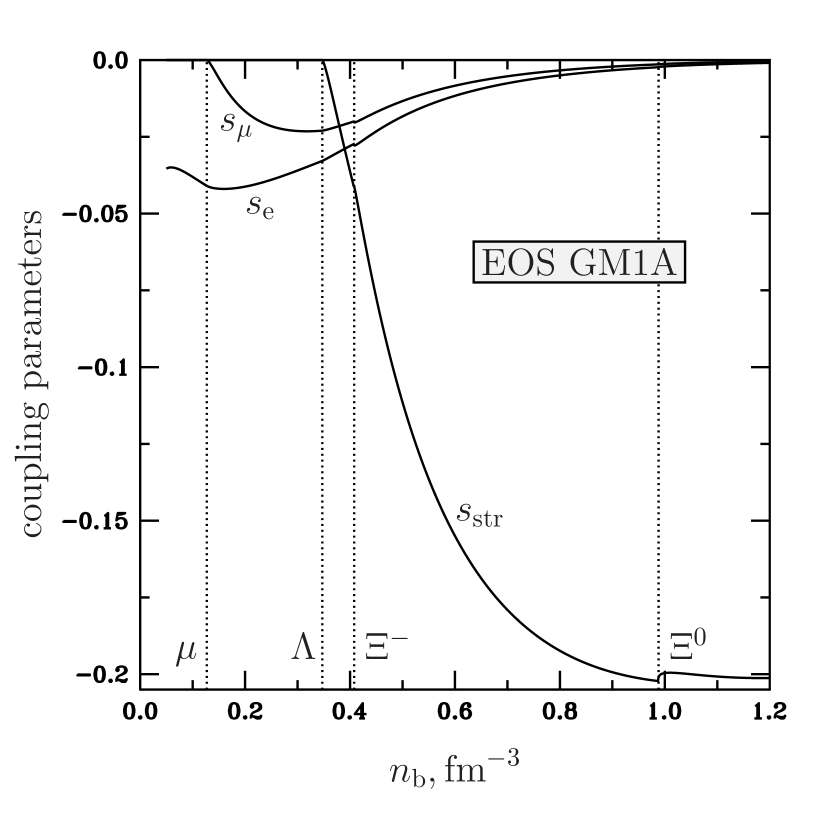
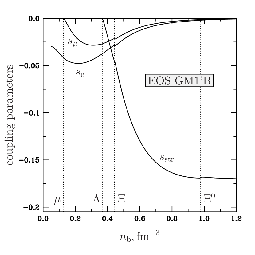
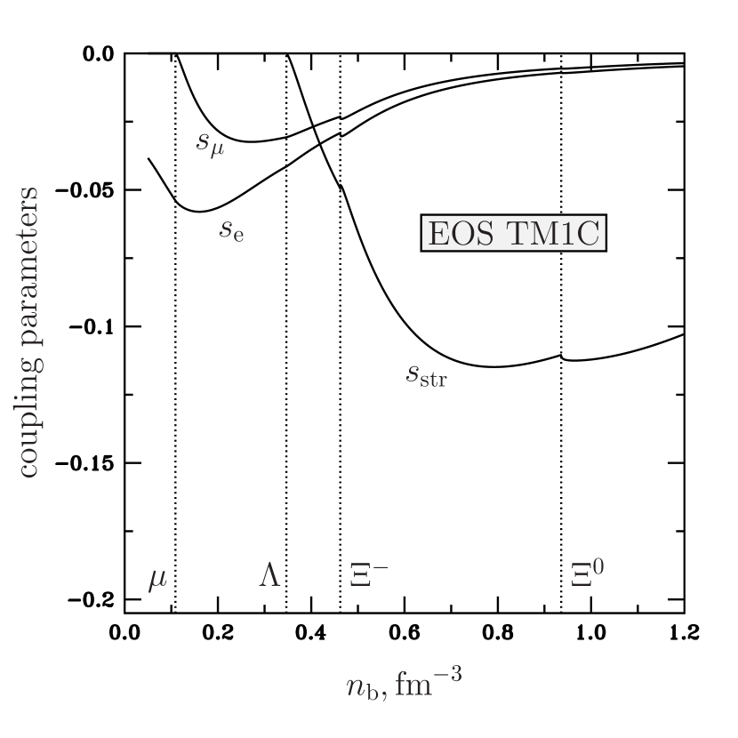
Figure 1: Coupling parameters $s_{\rm e},~{}s_{\rm\mu},~{}s_{\rm str}$ versus the baryon number density $n_{\rm b}$ for the EOSs GM1A, GM1’B, TM1C from Gusakov et al. (2014). Vertical lines are the thresholds for the appearance of muons and $\rm\Lambda$–, ${\rm\Xi}^{-}$–, ${\rm\Xi}^{0}$–hyperons.

3.3 Superfluid equations

Assuming that all the coupling parameters vanish, one can, in principle, study superfluid oscillation modes using the potentiality conditions for the motion of superfluid components (24) together with the continuity equations (16) and the condition $\delta U_{({\rm b})}^{\alpha}=\delta g^{\alpha\beta}=0$ (as it is discussed in the previous section). However, if the coupling parameters are small but finite (which is the case for realistic EOSs), such an approach will lead to significant errors (see details in Appendix A). In this section we derive a set of equations which are more suitable for our decoupling scheme. These equations are generalization of the superfluid equation discussed by Gusakov & Kantor (2011). To obtain them, we follow the derivation of that paper.

Using the energy-momentum conservation (22), one can compose a vanishing combination ${{T_{\alpha}}^{\beta}}\phantom{}_{;\beta}+u_{\alpha}u_{\gamma}{T^{\gamma\beta}}\phantom{}_{;\beta}=0$. Subtracting from it the potentiality condition (24) for neutrons multiplied by $n_{\rm b}u^{\beta}$, one obtains

$$(P+\varepsilon-\mu_{\rm n}n_{\rm b})u^{\beta}{u_{\alpha}}\phantom{}_{;\beta}+\left(\partial_{\beta}{P}-n_{\rm b}\partial_{\beta}{\mu_{\rm n}}\right)u_{\alpha}u^{\beta}+\left(\partial_{\alpha}{P}-n_{\rm b}\partial_{\alpha}{\mu_{\rm n}}\right)\\ +(g_{\alpha\gamma}+u_{\alpha}u_{\gamma})u^{\beta}{(\mu_{\rm n}n_{\rm b}W^{\gamma})}\phantom{}_{;\beta}+\mu_{\rm n}n_{\rm b}\left({{u^{\beta}}}\phantom{}_{;\beta}W_{\alpha}+{u_{\alpha}}\phantom{}_{;\beta}W^{\beta}\right)-n_{\rm b}u^{\beta}\left[{w_{({\rm n})\alpha}}\phantom{}_{;\beta}-{w_{({\rm n})\beta}}\phantom{}_{;\alpha}\right]=0,$$ (51)

or, using the thermodynamic relations (31) and (33),

$$\left(-\Delta\mu_{\rm e}n_{\rm e}-\Delta\mu_{\rm\mu}n_{\rm\mu}-\Delta\mu_{\rm\Lambda}n_{\rm str}\right)u^{\beta}{u_{\alpha}}\phantom{}_{;\beta}+\left(-n_{\rm e}\partial_{\beta}{\Delta\mu_{\rm e}}-n_{\rm\mu}\partial_{\beta}{\Delta\mu_{\rm\mu}}-n_{\rm str}\partial_{\beta}{\Delta\mu_{\rm\Lambda}}\right)u_{\alpha}u^{\beta}\\ +\left(-n_{\rm e}\partial_{\alpha}{\Delta\mu_{\rm e}}-n_{\rm\mu}\partial_{\alpha}{\Delta\mu_{\rm\mu}}-n_{\rm str}\partial_{\alpha}{\Delta\mu_{\rm\Lambda}}\right)+(g_{\alpha\gamma}+u_{\alpha}u_{\gamma})u^{\beta}{(\mu_{\rm n}n_{\rm b}W^{\gamma})}\phantom{}_{;\beta}+\mu_{\rm n}n_{\rm b}\left({{u^{\beta}}}\phantom{}_{;\beta}W_{\alpha}+{u_{\alpha}}\phantom{}_{;\beta}W^{\beta}\right)\\ -n_{\rm b}u^{\beta}\left[{w_{({\rm n})\alpha}}\phantom{}_{;\beta}-{w_{({\rm n})\beta}}\phantom{}_{;\alpha}\right]=0.$$ (52)

Each term in equation (52) depends on one of the small quantities $\Delta\mu_{\rm e}$, $\Delta\mu_{\rm\mu}$, $\Delta\mu_{\rm\Lambda}$, $w_{({\rm n})}^{\alpha}$ or $W^{\alpha}$. Thus, since we are working in the linear approximation, one can replace all other quantities in this equation with their equilibrium values.

Now let us consider a non-rotating equilibrated star with the Schwarzschild metric,

$${\rm d}s^{2}=-{\rm e}^{\nu}{\rm d}t^{2}+{\rm e}^{\lambda}{\rm d}r^{2}+r^{2}({\rm d}\theta^{2}+\sin^{2}\theta{\rm d}\phi^{2}),$$ (53)

and assume that all its perturbations depend on time as ${\rm e}^{{\rm i}\omega t}$ ($\omega$ is the perturbation frequency). In this case the spatial components ($\alpha=1,\,2,\,3$) of the superfluid equation take a very simple form

$${\rm i}\omega n_{\rm b}(\mu_{\rm n}W_{\alpha}-w_{({\rm n})\alpha})=n_{\rm e}\frac{\partial}{\partial x^{\alpha}}\left(\Delta\mu_{\rm e}{\rm e}^{\nu/2}\right)+n_{\rm\mu}\frac{\partial}{\partial x^{\alpha}}\left(\Delta\mu_{\rm\mu}{\rm e}^{\nu/2}\right)+n_{\rm str}\frac{\partial}{\partial x^{\alpha}}\left(\Delta\mu_{\rm\Lambda}{\rm e}^{\nu/2}\right),\quad\alpha=1,2,3.$$ (54)

In a similar way (using the potentiality condition for $\rm\Lambda$–hyperons instead of neutrons) one can derive an equation for $\rm\Lambda$–hyperons,

$${\rm i}\omega n_{\rm b}(\mu_{\rm n}W_{\alpha}-w_{({\rm\Lambda})\alpha})=n_{\rm e}\frac{\partial}{\partial x^{\alpha}}\left(\Delta\mu_{\rm e}{\rm e}^{\nu/2}\right)+n_{\rm\mu}\frac{\partial}{\partial x^{\alpha}}\left(\Delta\mu_{\rm\mu}{\rm e}^{\nu/2}\right)+(n_{\rm str}-n_{\rm b})\frac{\partial}{\partial x^{\alpha}}\left(\Delta\mu_{\rm\Lambda}{\rm e}^{\nu/2}\right),\quad\alpha=1,2,3.$$ (55)

Subtracting equation (55) from (54), one can obtain the following simple equation:

$${\rm i}\omega n_{\rm b}(w_{({\rm\Lambda})\alpha}-w_{({\rm n})\alpha})=n_{\rm b}\frac{\partial}{\partial x^{\alpha}}\left(\Delta\mu_{\rm\Lambda}{\rm e}^{\nu/2}\right),\quad\alpha=1,2,3.$$ (56)

This equation could also be derived by subtracting the potentiality condition for neutrons from the potentiality condition for $\rm\Lambda$–hyperons (see equation 24).

As a result, superfluid oscillation modes in the decoupling regime can be calculated by using the two equations, (54) and (56), along with the continuity equations (16) and the conditions $\delta U_{({\rm b})}^{\alpha}=\delta g^{\alpha\beta}=0$. If neutrons or $\rm\Lambda$–hyperons are non-superfluid, one can write similar equations for other particle species (see Appendix B for more details).

3.4 Effects of rotation

Rotation leads to the formation of Feynman-Onsager vortices inside HSs with the interspacing distance $\sim 10^{-2}-10^{-4}{\rm cm}$. Neglecting the vortex energy, the hydrodynamic equations averaged over the volume containing large amount of vortices have the same form as the corresponding equations for non-rotating matter (Khalatnikov & Bekarevich 1961; Mendell & Lindblom 1991). The only exception is the potentiality condition (24), which should be replaced (for neutral particles) by

$$u^{\beta}\left[{\left(w_{(i)\beta}+\mu_{i}u_{\beta}\right)}\phantom{}_{;\alpha}-{\left(w_{(i)\alpha}+\mu_{i}u_{\alpha}\right)}\phantom{}_{;\beta}\right]=\mu_{\rm n}n_{\rm b}f_{\alpha(i)}.$$ (57)

This equation is a generalization of equation (8) from Kantor & Gusakov (2012) to the case of a few neutral superfluids. The vector $f_{\alpha(i)}$ here is defined as

$$f_{(i)}^{\alpha}=\alpha_{i}(g^{\alpha\beta}+u^{\alpha}u^{\beta})F_{\beta\gamma(i)}W_{(i)}^{\gamma}+\frac{\beta_{i}-\gamma_{i}}{N_{i}}\left[F_{\gamma\beta(i)}F_{(i)}^{\beta\alpha}+u^{\alpha}u_{\delta}F_{\gamma\beta(i)}F_{(i)}^{\beta\delta}+u^{\beta}u_{\delta}F_{\gamma\beta(i)}F_{(i)}^{\delta\alpha}\right]W_{(i)}^{\gamma}+\gamma_{i}N_{i}W_{(i)}^{\alpha},$$ (58)

where no summation over index $i$ is assumed, and

$$W_{(i)}^{\alpha}\equiv\frac{Y_{ik}w_{(k)}^{\alpha}}{n_{\rm b}},$$ (59)

$$F_{\alpha\beta(i)}={\left(w_{(i)\beta}+\mu_{i}u_{\beta}\right)}\phantom{}_{;\alpha}-{\left(w_{(i)\alpha}+\mu_{i}u_{\alpha}\right)}\phantom{}_{;\beta},$$ (60)

$$N_{i}=\left(-\frac{1}{2}F_{\alpha\beta(i)}F_{(i)}^{\alpha\beta}-u^{\alpha}u_{\gamma}F_{\beta\alpha(i)}F_{(i)}^{\beta\gamma}\right)^{1/2}.$$ (61)

Here $\alpha_{i}$, $\beta_{i}$, and $\gamma_{i}$ are some scalars (kinetic coefficients), which, in the non-relativistic limit, are equal to the corresponding coefficients of non-relativistic hydrodynamics describing a rotating superfluid (see Khalatnikov & Bekarevich 1961).

Let us now inspect how rotation affects the oscillation equations. The right-hand side of equation (57) can schematically be presented in the form $\mu_{\rm n}n_{\rm b}f_{\alpha(i)}\equiv O_{\alpha\beta(i)}W_{(i)}^{\beta}$, where the tensor $O^{\alpha\beta}_{(i)}$ is defined by the expression (58) for $f^{\alpha}_{(i)}$. Repeating now the derivation of equation (52) and making use of Eq. (57) instead of the potentiality condition (24), one derives the same equation (52) but with the term $n_{\rm b}O_{\alpha\beta({\rm n})}W_{({\rm n})}^{\beta}$ in its right-hand side. This term depends on the small quantity $W_{({\rm n})}^{\beta}$, vanishing in equilibrium, so that our reasoning about the mode decoupling remains valid even for the rotating HSs. Note that, allowing for rotation, one should use the metric of a rotating star instead of the Schwarzschild metric.

Superfluid oscillation modes (e.g., superfluid r-modes) in a rotating HS are described by the following equations for the superfluid velocities $w_{({\rm n})}^{\alpha}$ and $w_{({\rm\Lambda})}^{\alpha}$ (both neutrons and $\Lambda$–hyperons are assumed to be superfluid):

$$\left(-\Delta\mu_{\rm e}n_{\rm e}-\Delta\mu_{\rm\mu}n_{\rm\mu}-\Delta\mu_{\rm\Lambda}n_{\rm str}\right)u^{\beta}{u_{\alpha}}\phantom{}_{;\beta}+\left(-n_{\rm e}\partial_{\beta}{\Delta\mu_{\rm e}}-n_{\rm\mu}\partial_{\beta}{\Delta\mu_{\rm\mu}}-n_{\rm str}\partial_{\beta}{\Delta\mu_{\rm\Lambda}}\right)u_{\alpha}u^{\beta}\\ +\left(-n_{\rm e}\partial_{\alpha}{\Delta\mu_{\rm e}}-n_{\rm\mu}\partial_{\alpha}{\Delta\mu_{\rm\mu}}-n_{\rm str}\partial_{\alpha}{\Delta\mu_{\rm\Lambda}}\right)+(g_{\alpha\gamma}+u_{\alpha}u_{\gamma})u^{\beta}{(\mu_{\rm n}n_{\rm b}W^{\gamma})}\phantom{}_{;\beta}+\mu_{\rm n}n_{\rm b}\left({{u^{\beta}}}\phantom{}_{;\beta}W_{\alpha}+{u_{\alpha}}\phantom{}_{;\beta}W^{\beta}\right)\\ -n_{\rm b}u^{\beta}\left[{w_{({\rm n})\alpha}}\phantom{}_{;\beta}-{w_{({\rm n})\beta}}\phantom{}_{;\alpha}\right]=n_{\rm b}O_{\alpha\beta({\rm n})}W_{({\rm n})}^{\beta},$$ (62)

$$\left(-\Delta\mu_{\rm e}n_{\rm e}-\Delta\mu_{\rm\mu}n_{\rm\mu}-\Delta\mu_{\rm\Lambda}n_{\rm str}+\Delta\mu_{\rm\Lambda}n_{\rm b}\right)u^{\beta}{u_{\alpha}}\phantom{}_{;\beta}+\left(-n_{\rm e}\partial_{\beta}{\Delta\mu_{\rm e}}-n_{\rm\mu}\partial_{\beta}{\Delta\mu_{\rm\mu}}-n_{\rm str}\partial_{\beta}{\Delta\mu_{\rm\Lambda}}+n_{\rm b}\partial_{\beta}{\Delta\mu_{\rm\Lambda}}\right)u_{\alpha}u^{\beta}\\ +\left(-n_{\rm e}\partial_{\alpha}{\Delta\mu_{\rm e}}-n_{\rm\mu}\partial_{\alpha}{\Delta\mu_{\rm\mu}}-n_{\rm str}\partial_{\alpha}{\Delta\mu_{\rm\Lambda}}+n_{\rm b}\partial_{\alpha}{\Delta\mu_{\rm\Lambda}}\right)+(g_{\alpha\gamma}+u_{\alpha}u_{\gamma})u^{\beta}{(\mu_{\rm n}n_{\rm b}W^{\gamma})}\phantom{}_{;\beta}+\mu_{\rm n}n_{\rm b}\left({{u^{\beta}}}\phantom{}_{;\beta}W_{\alpha}+{u_{\alpha}}\phantom{}_{;\beta}W^{\beta}\right)\\ -n_{\rm b}u^{\beta}\left[{w_{({\rm\Lambda})\alpha}}\phantom{}_{;\beta}-{w_{({\rm\Lambda})\beta}}\phantom{}_{;\alpha}\right]=n_{\rm b}O_{\alpha\beta({\rm\Lambda})}W_{({\rm\Lambda})}^{\beta}.$$ (63)

As in the previous section, all the quantities in equations (62) and (63) except for $\Delta\mu_{\rm e}$, $\Delta\mu_{\rm\mu}$, $\Delta\mu_{\rm\Lambda}$, $w_{(i)}^{\alpha}$, and $W_{(i)}^{\alpha}$ should be replaced with their equilibrium values.

4 Example: sound waves in nucleon-hyperon matter

In this section we illustrate the decoupling scheme developed in Section 3 by the calculation of the speed of sound in a homogeneous nucleon–hyperon matter. Since this problem can be solved exactly, we can use it as a test for our approximate method. We consider small harmonic perturbations ($\sim{\rm e}^{{\rm i}\omega t-{\rm i}\boldsymbol{kr}}={\rm e}^{-{\rm i}k_{\alpha}x^{\alpha}}$) in homogeneous superfluid matter in Minkowski spacetime with the metric $g^{\alpha\beta}=\operatorname{diag}(-1,1,1,1)$. We assume that all baryons ($\rm n$, $\rm p$, $\rm\Lambda$, ${\rm\Xi}^{-}$, ${\rm\Xi}^{0}$, ${\rm\Sigma}^{-}$) can be superfluid.

Perturbations are described by the energy-momentum conservation law (22) and superfluid equations (54) and (55) for neutrons and $\rm\Lambda$–hyperons. In our case these equations take the following simple form:

$$\omega(P+\varepsilon)\boldsymbol{\delta U}_{({\rm b})}=\boldsymbol{k}\delta P,$$ (64)

$$\omega n_{\rm b}\left(\mu_{\rm n}\boldsymbol{W}-\boldsymbol{w}_{({\rm n})}\right)=-\boldsymbol{k}\left(n_{\rm e}\Delta\mu_{\rm e}+n_{\rm\mu}\Delta\mu_{\rm\mu}+n_{{\rm str}}\Delta\mu_{\rm\Lambda}\right),$$ (65)

$$\omega n_{\rm b}\left(\mu_{\rm n}\boldsymbol{W}-\boldsymbol{w}_{({\rm\Lambda})}\right)=-\boldsymbol{k}\left(n_{\rm e}\Delta\mu_{\rm e}+n_{\rm\mu}\Delta\mu_{\rm\mu}+n_{\rm str}\Delta\mu_{\rm\Lambda}-n_{\rm b}\Delta\mu_{\rm\Lambda}\right).$$ (66)

Here $\boldsymbol{\delta U}_{({\rm b})}$, $\boldsymbol{W}$, $\boldsymbol{w}_{(i)}$, and $\boldsymbol{k}$ are three-vectors composed of spatial components of the corresponding four-vectors.

Now we have to write $\delta P$ and $\Delta\mu_{j}$ in terms of $\boldsymbol{\delta U}_{({\rm b})}$, $\boldsymbol{w}_{({\rm n})}$, and $\boldsymbol{w}_{({\rm\Lambda})}$. As a first step, we present them as functions of the number density perturbations,

$$\delta=\delta n_{\rm b}\frac{\partial}{\partial n_{\rm b}}+\delta n_{\rm e}\frac{\partial}{\partial n_{\rm e}}+\delta n_{\rm\mu}\frac{\partial}{\partial n_{\rm\mu}}+\delta n_{{\rm str}}\frac{\partial}{\partial n_{{\rm str}}},$$ (67)

and then, with the help of the continuity equations (15) and (16), express the number density perturbations through the velocities $\boldsymbol{\delta U}_{({\rm b})}$ and $\boldsymbol{w}_{(i)}$:

$$\delta n_{\rm b}=n_{\rm b}\frac{\boldsymbol{k}}{\omega}\boldsymbol{\delta U}_{({\rm b})},$$ (68)

$$\delta n_{\rm e}=n_{\rm e}\frac{\boldsymbol{k}}{\omega}\boldsymbol{\delta u}=n_{\rm e}\frac{\boldsymbol{k}}{\omega}\left(\boldsymbol{\delta U}_{({\rm b})}-\frac{1}{n_{\rm b}}\sum_{i}Y_{ik}\boldsymbol{w}_{(k)}\right),$$ (69)

$$\delta n_{\rm\mu}=n_{\rm\mu}\frac{\boldsymbol{k}}{\omega}\boldsymbol{\delta u}=n_{\rm\mu}\frac{\boldsymbol{k}}{\omega}\left(\boldsymbol{\delta U}_{({\rm b})}-\frac{1}{n_{\rm b}}\sum_{i}Y_{ik}\boldsymbol{w}_{(k)}\right),$$ (70)

$$\delta n_{{\rm str}}=n_{{\rm str}}\frac{\boldsymbol{k}}{\omega}\boldsymbol{\delta U}_{({\rm str})}=\frac{\boldsymbol{k}}{\omega}\left[n_{{\rm str}}\boldsymbol{\delta U}_{({\rm b})}-\frac{n_{{\rm str}}}{n_{\rm b}}\sum_{i}Y_{ik}\boldsymbol{w}_{(k)}-S_{i}Y_{ik}\boldsymbol{w}_{(k)}\right].$$ (71)

Also we should express all the superfluid velocities $\boldsymbol{w}_{(k)}$ through $\boldsymbol{w}_{({\rm n})}$ and $\boldsymbol{w}_{({\rm\Lambda})}$ using Eqs. (19) and (37)–(39).

After substituting all these relations into the system of equations (64)–(66) one arrives at the linear equation of the form

$$\mathsf{\mathbf{A}}\cdot\boldsymbol{x}=0,$$ (72)

where $\boldsymbol{x}$ is a vector, $\boldsymbol{x}=(\delta U_{({\rm b})},w_{({\rm n})},w_{({\rm\Lambda})})$, with $\delta U_{({\rm b})}=\boldsymbol{\delta U}_{({\rm b})}\boldsymbol{k}/k$, $w_{({\rm n})}=\boldsymbol{w}_{({\rm n})}\boldsymbol{k}/k$, and $w_{({\rm\Lambda})}=\boldsymbol{w}_{({\rm\Lambda})}\boldsymbol{k}/k$ (it is clear that the vectors $\boldsymbol{k}$, $\boldsymbol{\delta U}_{({\rm b})}$, $\boldsymbol{w}_{({\rm n})}$ and $\boldsymbol{w}_{({\rm\Lambda})}$ must be collinear); $\mathsf{\mathbf{A}}$ is a $3\times 3$ matrix, whose elements depend on thermodynamic quantities, entrainment matrix $Y_{ik}$, as well as on the frequency $\omega$ and the wavenumber $k$. The system (72) has a nontrivial solution only if $\det\mathsf{\mathbf{A}}=0$. This condition results in a cubic equation for the squared speed of sound, $c_{\rm S}^{2}\equiv\omega^{2}/k^{2}$. Three roots of this cubic equation correspond to three sound modes in the nucleon–hyperon matter.

Note that in the decoupling approximation $\delta P$ does not depend on $\delta n_{\rm e(SFL)}$, $\delta n_{\rm\mu(SFL)}$, and $\delta n_{\rm str(SFL)}$ (see equation 49), so that Eq. (64) coincides with the corresponding equation for the normal (non-superfluid) matter and does not contain the superfluid variables $\boldsymbol{w}_{(i)}$. This equation describes ‘normal’ sound modes and can be solved separately from equations (65) and (66). The latter equations describe ‘superfluid’ sound modes.

We calculated sound speeds for the EOSs GM1A, GM1’B, and TM1C studied by Gusakov et al. (2014). In our calculations we need to specify baryon critical temperatures $T_{{\rm c}i}$, which are generally functions of baryon number density $n_{\rm b}$. These temperatures are poorly known, especially for hyperons (see e.g., Page et al. 2013). In view of large uncertainties, we (somewhat arbitrary) adopt the following values for $T_{{\rm c}i}$: $T_{\rm cn}=5\times 10^{8}~{}{\rm K}$, $T_{\rm cp}=3\times 10^{9}~{}{\rm K}$, $T_{\rm c\Xi^{-}}=T_{\rm c\Xi^{0}}=5\times 10^{9}~{}{\rm K}$. These values do not contradict the results of microscopic calculations (see e.g., Yakovlev et al. 1999; Lombardo & Schulze 2001; Page et al. 2013; Gezerlis et al. 2014 and references therein).

As for $\rm\Lambda$–hyperons, we consider two different possibilities discussed in the literature (see e.g., Takatsuka et al. 2006; Wang & Shen 2010):

1. $\rm\Lambda$–hyperons are superfluid, $T_{\rm c\Lambda}=10^{9}\,{\rm K}$. The dependence of the sound speeds $c_{\rm S}$ on the baryon number density $n_{\rm b}$ and on the temperature $T$ for this case is shown in Figs. 2 and 4, respectively.

2. $\rm\Lambda$–hyperons are normal at $T>10^{7}\,{\rm K}$. The corresponding functions $c_{\rm S}(n_{\rm b})$ and $c_{\rm S}(T)$ are demonstrated in Figs. 3 and 5, respectively.

Let us discuss Figs. 2–5 in more detail. Fig. 2 shows the dependence $c_{\rm S}(n_{\rm b})$ at fixed $T=3\times 10^{7}~{}{\rm K}$ for the first case ($T_{\rm c\Lambda}=10^{9}\,{\rm K}$). The solid lines present sound speeds calculated in the decoupling approximation, the dashed lines show the exact results. The vertical lines denote the thresholds for appearance of different particle species. The highest sound speed on every plot is labelled ‘normal’, because in the fully decoupled case it coincides with the sound speed in the non-superfluid matter. Other modes appear only in superfluid matter and are therefore labelled ‘SFL’. The number of superfluid sound modes is equal to the number of superfluid degrees of freedom, as discussed in Section 2.4. The second superfluid mode arises after the appearance of $\rm\Lambda$–hyperons. Note that the appearance of ${\rm\Xi}^{-}$ or ${\rm\Xi}^{0}$–hyperons does not lead to any additional degrees of freedom (and, hence, to new sound modes) due to the constraints (37) and (38).

Fig. 3 presents a similar plot but for non-superfluid $\rm\Lambda$–hyperons (case ii). Since $\rm\Lambda$–hyperons are normal, the second superfluid degree of freedom (associated with a ‘quasiparticle’ $A=({\rm p}+{\rm\Xi}^{-})/2$ and its superfluid four-vector $w_{(A)\alpha}=(w_{({\rm p})\alpha}+w_{({\rm\Xi}^{-})\alpha})/2$; see Appendix B) exists only in the presence of ${\rm\Xi}^{-}$–hyperons. Note that the second superfluid sound speed is much lower than in the case of superfluid $\rm\Lambda$–hyperons. In Figs. 2 and 3 (at low densities) one can see crossing of ‘normal’ and ‘SFL-I’ modes in the decoupling regime, while the exact solution shows the avoided crossing. This feature, generic to superfluid stars, was also observed e.g., by Gusakov & Kantor (2011) and Kantor & Gusakov (2011).

The dependence $c_{\rm S}(T)$ at fixed $n_{\rm b}=1.1~{}{\rm fm}^{-3}$ is shown for the cases of superfluid and non-superfluid $\rm\Lambda$–hyperons in Figs. 4 and 5, respectively. The vertical lines in the figures denote the critical temperatures $T_{{\rm c}i}$ for different baryon species. At high temperatures, when all baryons become non-superfluid, the ‘decoupled’ (normal) speed of sound is equal to the exact one (as it should be). The sound modes depend on $T$ because of the temperature dependence of the entrainment matrix $Y_{ik}$. The effect of finite temperatures on $Y_{ik}$ was discussed by Gusakov et al. (2009b). Since $Y_{ik}\rightarrow 0$ as $T\rightarrow T_{{\rm c}i}$, superfluid speeds of sound also decrease with increasing temperature. When protons become normal ($T_{\rm cp}<T<T_{{\rm c}{\rm\Xi}^{-}},~{}T_{{\rm c}{\rm\Xi}^{0}}$), only one superfluid mode (associated with ${\rm\Xi}^{0}$–hyperons) survives. One can see the avoided crossings of sound modes in Fig. 4.

To sum up, our numerical results show that the decoupling scheme developed in Section 3 allows one to calculate the oscillation modes within reasonable accuracy, which is determined by the coupling parameters $s_{\rm e}$, $s_{\rm\mu}$, and $s_{\rm str}$. At high densities the error is mainly due to the strange coupling parameter $s_{{\rm str}}$. For the EOS TM1C, $s_{{\rm str}}$ is smaller than that for the EOSs GM1A and GM1’B (see Fig. 1). That is why the difference between the exact and decoupled solution for the EOS TM1C is smaller.

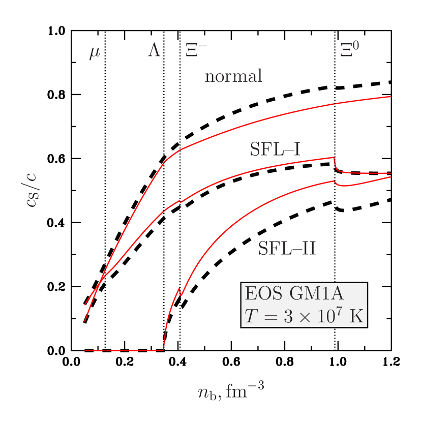
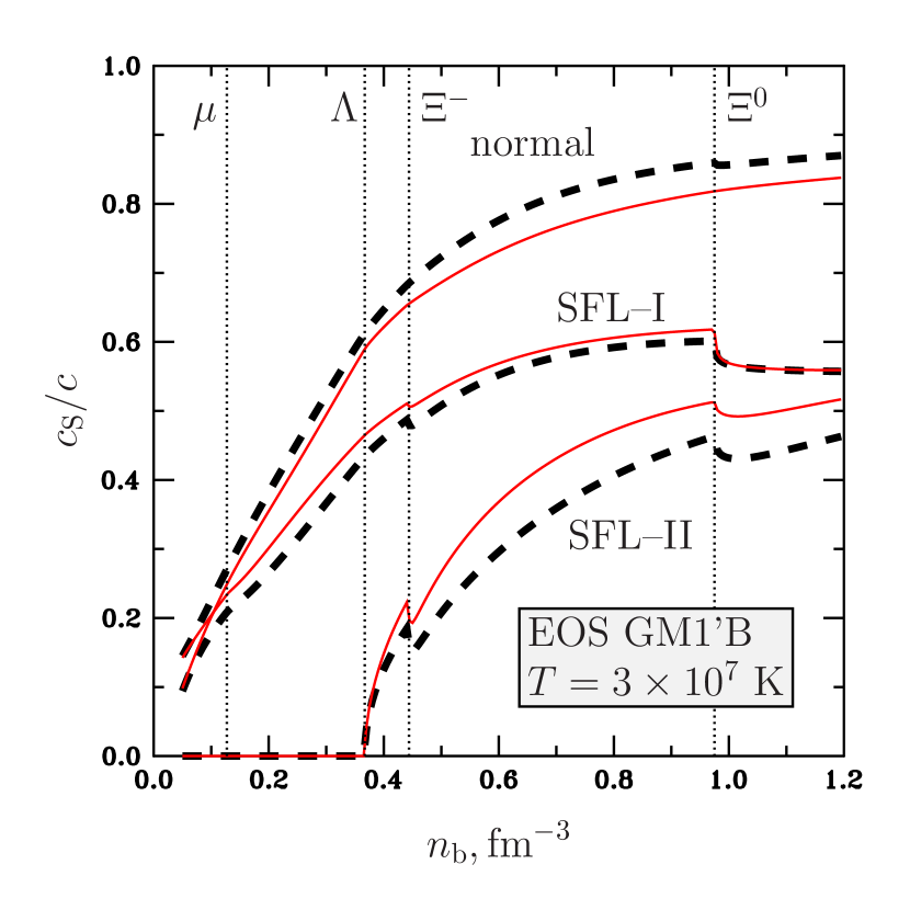
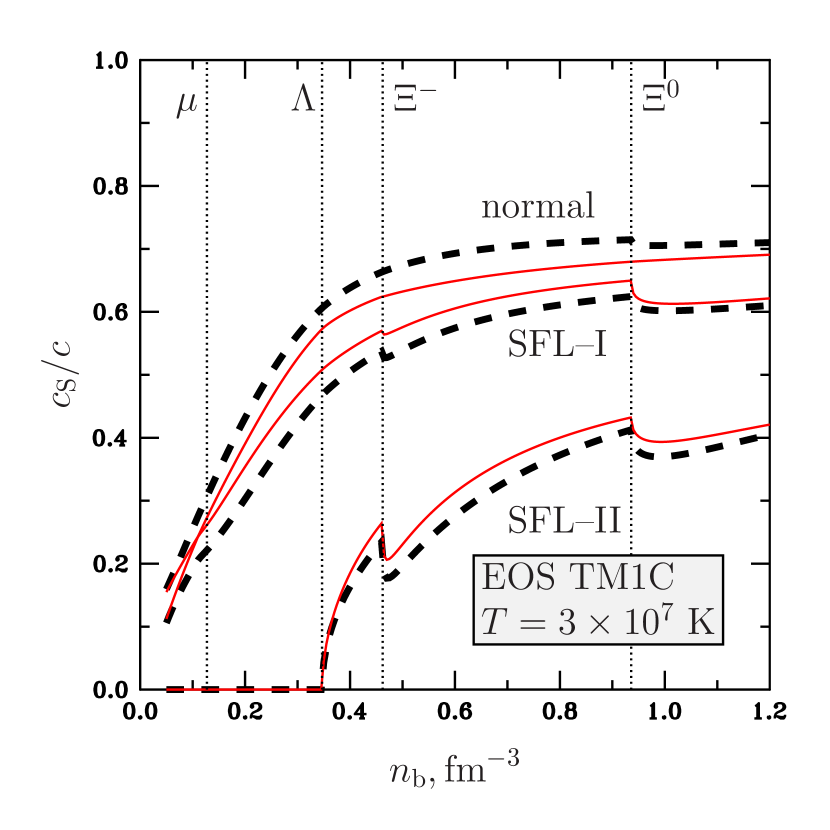
Figure 2: Speed of sound $c_{\rm S}$ (in units of $c$) versus the baryon number density $n_{\rm b}$ for the EOSs GM1A, GM1’B, TM1C at $T=3\times 10^{7}~{}{\rm K}$. Dashed lines: exact solution. Solid lines: decoupled solution. Vertical lines: thresholds for the appearance of muons and $\rm\Lambda$–, ${\rm\Xi}^{-}$–, ${\rm\Xi}^{0}$–hyperons. $\rm\Lambda$–hyperons are superfluid.

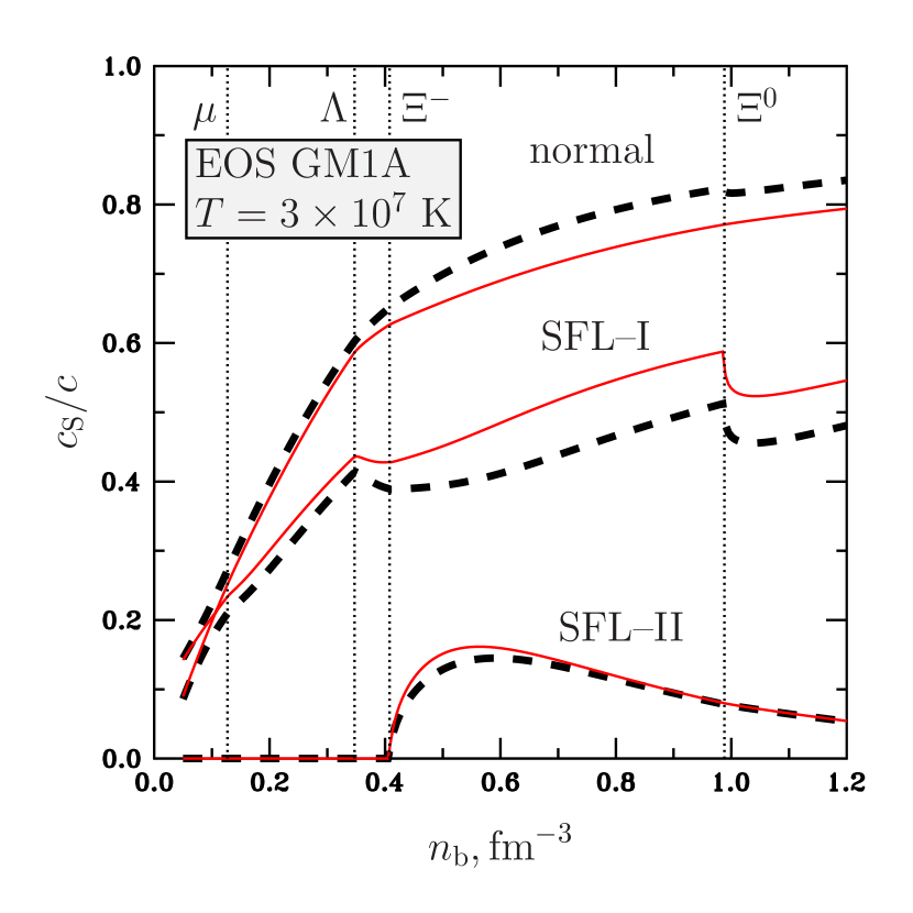
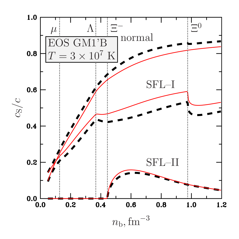
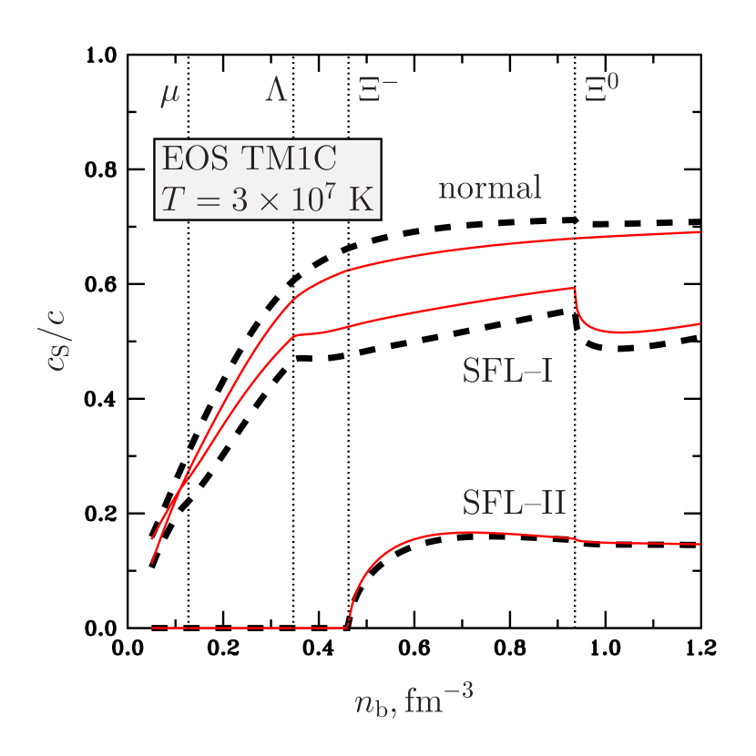
Figure 3: Speed of sound $c_{\rm S}$ (in units of $c$) versus the baryon number density $n_{\rm b}$ for the EOSs GM1A, GM1’B, TM1C at $T=3\times 10^{7}~{}{\rm K}$. Dashed lines: exact solution. Solid lines: decoupled solution. Vertical lines: thresholds for the appearance of muons and $\rm\Lambda$–, ${\rm\Xi}^{-}$–, ${\rm\Xi}^{0}$–hyperons. $\rm\Lambda$–hyperons are non-superfluid.

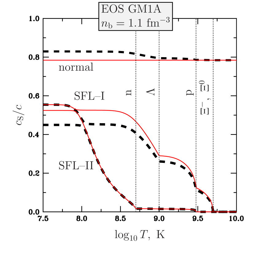
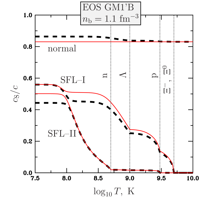
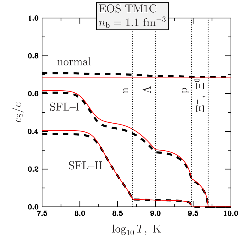
Figure 4: Speed of sound $c_{\rm S}$ (in units of $c$) versus temperature $\log_{10}T,~{}{\rm K}$ for the EOSs GM1A, GM1’B, TM1C at $n_{\rm b}=1.1\;{\rm fm^{-3}}$. Dashed lines: exact solution. Solid lines: decoupled solution. Vertical lines: critical temperatures for baryons. $\rm\Lambda$–hyperons are superfluid.

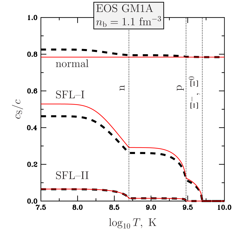
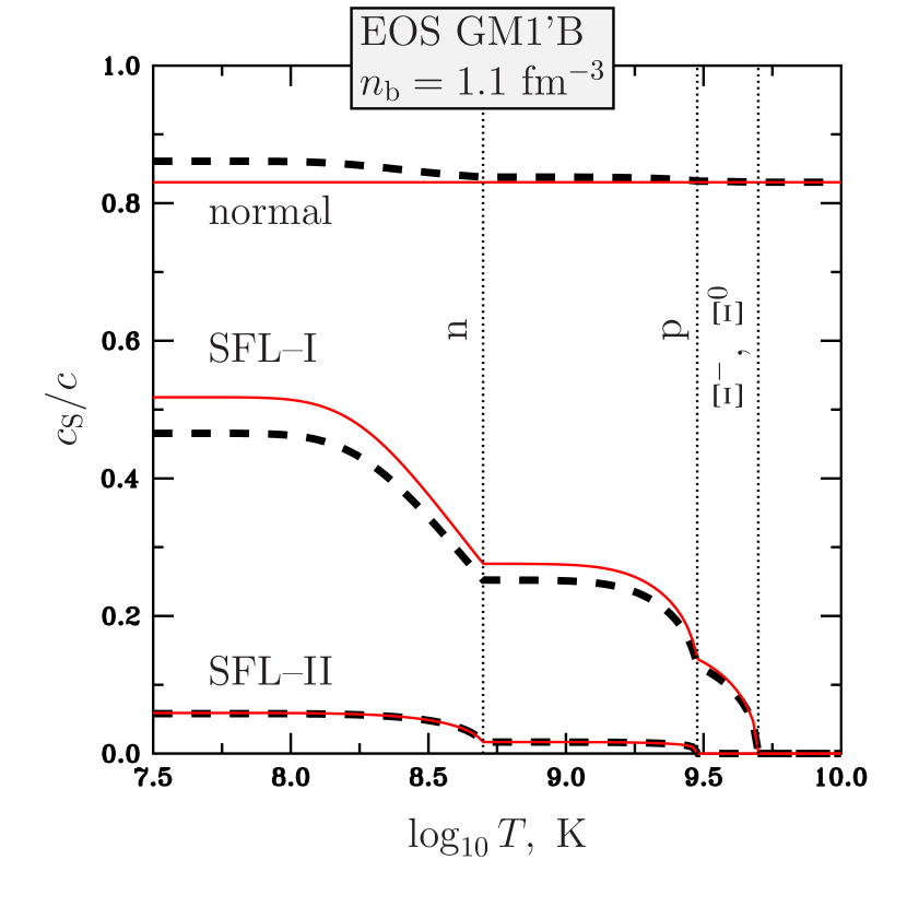
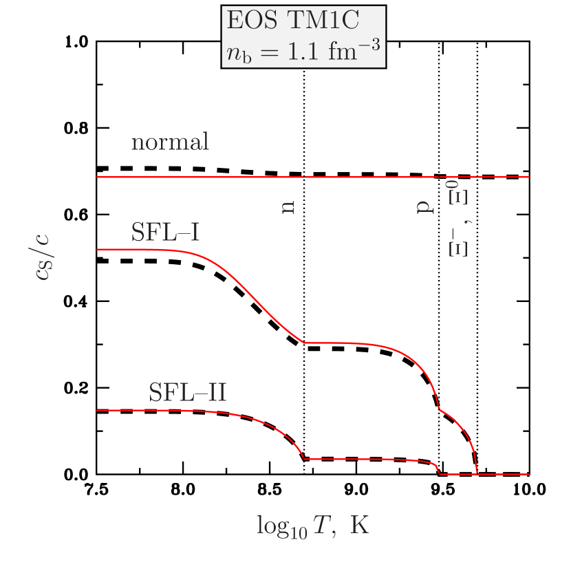
Figure 5: Speed of sound $c_{\rm S}$ (in units of $c$) versus temperature $\log_{10}T,~{}{\rm K}$ for the EOSs GM1A, GM1’B, TM1C at $n_{\rm b}=1.1\;{\rm fm^{-3}}$. Dashed lines: exact solution. Solid lines: decoupled solution. Vertical lines: critical temperatures for baryons. $\rm\Lambda$–hyperons are non-superfluid.

5 Composition g-modes in superfluid nucleon–hyperon matter

The decoupling scheme developed and applied in the preceding sections can be used to calculate various oscillation modes of superfluid HSs, e.g., f-, p-, and r-modes. We postpone a detailed analysis of superfluid oscillation modes in the nucleon-hyperon matter for a future publication.

However, there is an important class of oscillations, namely, the gravity modes (g-modes), that cannot be analysed within the framework presented above. It is easily verified that in the decoupling regime the g-modes exist and coincide with the g-modes of a non-superfluid HS. This is so ‘by construction’, because the decoupled equations, which describe the normal modes, are exactly the same as those for a non-superfluid star. Unfortunately, this result is completely wrong: the local analysis of hydrodynamic equations and numerical modelling show that the normal-like g-modes are artefacts of the adopted approximation. Putting it differently, the decoupling approximation is too crude to find the real g-modes. This conclusion is not surprising. For example, for a zero-temperature non-superfluid neutron star with the $\rm npe$ composition of the core, the g-modes disappear from the oscillation spectrum if one neglects the dependence of the pressure $P$ on the electron number density $n_{\rm e}$ (thus effectively treating a star as barotropic). In the decoupling approximation we also neglect the terms of this kind so that it is reasonable to expect that this affects the g-modes somehow. The fact that the g-modes in superfluid stars will differ substantially from their normal counterparts also clearly follows from the thought experiment discussed in the section II in Kantor & Gusakov (2014).

Meanwhile, the g-modes constitute a very interesting class of oscillations, especially because it has been believed, until recently, that they do not exist in the zero-temperature superfluid neutron stars (see e.g., Lee 1995; Andersson & Comer 2001; Prix & Rieutord 2002). However, as demonstrated by Kantor & Gusakov, this is generally not true (see also Passamonti et al. 2015). The g-modes, for example, can be excited in a superfluid $\rm npe\mu$ matter and their frequencies can be unusually large, up to $\sim 450$ Hz (while the frequencies of the ordinary composition g-modes in the non-superfluid neutron stars do not exceed $50-150$ Hz; see e.g., Reisenegger & Goldreich 1992). To the best of our knowledge, these modes have never been studied for nucleon-hyperon matter, even for non-superfluid HSs. This provides the motivation to study them here.

In this section, in all numerical calculations we employ the EOS GM1’B in the HS core and the EOS BSk21 (Potekhin et al. 2013) in the crust. All numerical results are obtained for a neutron star with the mass $M=1.634~{}\rm M_{\odot}$, the radius $R=13.55~{}{\rm km}$, and the central density $\rho_{\rm c}=8.1\times 10^{14}\rm~{}g~{}cm^{-3}$. The threshold for the $\rm\Lambda$–hyperon appearance in such star lies at a distance $r\approx 5.29\rm~{}km$ from the centre; other hyperons are absent. We assume that $\rm\Lambda$–hyperons are normal (case ii in Section 4), while the neutron and proton redshifted critical temperatures are constant throughout the core, $T_{\rm cn}^{\infty}\equiv T_{\rm cn}{\rm e}^{\nu/2}=5\times 10^{8}\rm K$ and $T_{\rm cp}^{\infty}\equiv T_{\rm cp}{\rm e}^{\nu/2}=3\times 10^{9}\rm K$. This simplifying assumption does not affect the g-mode spectrum in the limit $T^{\infty}\ll T_{\rm cn}^{\infty}$ ($T^{\infty}$ is the redshifted internal stellar temperature), when the g-mode frequencies reach a maximum value (Kantor & Gusakov 2014). It is the limit we are mostly interested in here.

5.1 Superfluid oscillation equations

We examine the superfluid g-modes following an approach presented recently by Kantor & Gusakov (2014). As mentioned above, we consider a model of a HS whose core consists of neutrons, protons, electrons, muons, and $\rm\Lambda$–hyperons ($\rm npe\mu\Lambda$ matter), assuming that neutrons and protons are superfluid, while $\rm\Lambda$–hyperons are not. We also assume that the metric is not perturbed during oscillations – this assumption, called the Cowling approximation (see Cowling 1941), works very well for the g-modes (see e.g., Gaertig & Kokkotas 2009). We consider non-radial perturbations $\propto{\rm e}^{{\rm i}\omega t}Y_{lm}(\theta,\phi)$ ($Y_{lm}$ is a spherical harmonic) of a non-rotating spherically symmetric star with the Schwarzschild metric (53). Equations, governing such perturbations in the $\rm npe\mu$ matter, were derived in the paper by Kantor & Gusakov (2014) (see equations 7–10 there). A straightforward generalization of these equations to the case of $\rm npe\mu\Lambda$ matter yields the following system of equations (the terms arising due to the presence of $\rm\Lambda$–hyperons are underlined):

$$\left(g\mu_{\rm n}n_{\rm b}\frac{\partial n_{\rm b}}{\partial P}+g\mu_{\rm n}\frac{\partial n_{\rm b}}{\partial\mu_{\rm n}}-\frac{\partial n_{\rm b}}{\partial x_{\rm e\mu}}\nabla x_{\rm e\mu}-\underline{\frac{\partial n_{\rm b}}{\partial x_{\rm e\Lambda}}\nabla x_{\rm e\Lambda}}\right)\,\xi^{r}_{(\rm b)}-\frac{n_{\rm b}}{{\rm e}^{\lambda/2}r^{2}}\frac{\partial}{\partial r}\left({\rm e}^{\lambda/2}r^{2}\xi^{r}_{(\rm b)}\right)+\frac{n_{\rm b}l(l+1){\rm e}^{\nu}}{r^{2}\omega^{2}(P+\varepsilon)}\delta P\\ =\frac{\partial n_{\rm b}}{\partial P}\delta P+\frac{\partial n_{\rm b}}{\partial\mu_{\rm n}}\delta\mu_{\rm n}-\frac{\partial n_{\rm b}}{\partial x_{\rm e\mu}}\nabla x_{\rm e\mu}\,\xi^{r}-\underline{\frac{\partial n_{\rm b}}{\partial x_{\rm e\Lambda}}\nabla x_{\rm e\Lambda}\,\xi^{r}},$$ (73)

$$-\omega^{2}\mu_{\rm n}n_{\rm b}{\rm e}^{\lambda-\nu}\xi_{(\rm b)}^{r}+\frac{\partial\delta P}{\partial r}+g\left(\frac{\partial w}{\partial P}\delta P+\frac{\partial w}{\partial\mu_{\rm n}}\delta\mu_{\rm n}-\frac{\partial w}{\partial x_{\rm e\mu}}\nabla x_{\rm e\mu}\xi^{r}-\underline{\frac{\partial w}{\partial x_{\rm e\Lambda}}\nabla x_{\rm e\Lambda}\xi^{r}}\right)=0,$$ (74)

$${\rm e}^{\nu/2}\frac{\partial}{\partial r}\left(\delta\mu_{\rm n}{\rm e}^{\nu/2}\right)-\omega^{2}{\rm e}^{\lambda}\mu_{\rm n}\left[(y+1)\xi_{(\rm b)}^{r}-y\xi^{r}\right]=0,$$ (75)

$$\left(g\mu_{\rm n}n_{\rm b}\frac{\partial n_{\rm e}}{\partial P}+g\mu_{\rm n}\frac{\partial n_{\rm e}}{\partial\mu_{\rm n}}\right)\,\xi^{r}-\frac{n_{\rm e}}{{\rm e}^{\lambda/2}r^{2}}\frac{\partial}{\partial r}\left({\rm e}^{\lambda/2}r^{2}\xi^{r}\right)+\frac{n_{\rm e}l(l+1){\rm e}^{\nu}}{r^{2}\omega^{2}y(P+\varepsilon)}\left[(y+1)\delta P-n_{\rm b}\delta\mu_{\rm n}\right]=\frac{\partial n_{\rm e}}{\partial P}\delta P+\frac{\partial n_{\rm e}}{\partial\mu_{\rm n}}\delta\mu_{\rm n}.$$ (76)

Here all the quantities except for $\xi^{r}$, $\xi_{({\rm b})}^{r}$, $\delta P$, and $\delta\mu_{\rm n}$ are taken in equilibrium. $\delta P$ and $\delta\mu_{\rm n}$ are the Eulerian perturbations of the pressure and the neutron chemical potential, respectively; $\nabla\equiv{\rm d}/{\rm d}r$; $g=\nabla\nu/2$; $w=P+\varepsilon$; $x_{\rm e\mu}=n_{\rm\mu}/n_{\rm e}$; $x_{\rm e\Lambda}=n_{\rm\Lambda}/n_{\rm e}$; and the parameter $y$ is expressed through the entrainment matrix $Y_{ik}$ as

$$y=\frac{n_{\rm b}Y_{\rm pp}}{\mu_{\rm n}\left(Y_{\rm nn}Y_{\rm pp}-Y_{\rm np}^{2}\right)}-1.$$ (77)

Finally, $\xi^{r}$ and $\xi_{({\rm b})}^{r}$ are the radial components of the Lagrangian displacements for the normal liquid component and baryons, respectively. They are defined by

$$u^{r}={\rm i}\omega{\rm e}^{-\nu/2}\xi^{r},\quad U_{({\rm b})}^{r}={\rm i}\omega{\rm e}^{-\nu/2}\xi_{({\rm b})}^{r}.$$ (78)

5.2 Non-superfluid equations and boundary conditions

Equations (73)–(76) describe the oscillations in the internal superfluid region of the star. To calculate the eigenfrequencies of global oscillations (or to calculate the g-mode spectrum of a non-superfluid star) one should also consider the equations governing the oscillations of the non-superfluid matter (see e.g., McDermott et al. 1983; Reisenegger & Goldreich 1992):

$$-\frac{1}{{\rm e}^{\lambda/2}r^{2}}\frac{\partial}{\partial r}\left[{\rm e}^{\lambda/2}r^{2}\xi_{(\rm b)}^{r}\right]+\frac{l(l+1){\rm e}^{\nu}}{r^{2}\omega^{2}}\frac{\delta P}{P+\varepsilon}-\frac{\delta P+\nabla P\,\xi_{(\rm b)}^{r}}{\gamma P}=0,$$ (79)

$$\frac{\partial\delta P}{\partial r}+g\left(1+\frac{1}{c_{\rm s}^{2}}\right)\delta P+{\rm e}^{\lambda-\nu}(P+\varepsilon)(\mathcal{N}_{\rm nsf}^{2}-\omega^{2})\xi_{(\rm b)}^{r}=0.$$ (80)

Here $\mathcal{N}_{\rm nsf}$ is the Brunt-V$\ddot{\rm a}$is$\ddot{\rm a}$l$\ddot{\rm a}$ frequency for the non-superfluid matter. In the (normal) core it is given by

$$\mathcal{N}_{\rm nsf}^{2}=g^{2}\,\left(\frac{1}{c_{\rm eq}^{2}}-\frac{1}{c_{s}^{2}}\right)\,{\rm e}^{\nu-\lambda},$$ (81)

where $c_{\rm eq}^{2}=\nabla P/(\mu_{\rm n}\nabla n_{\rm b})$; $c_{\rm s}^{2}\equiv\gamma P/(\mu_{\rm n}n_{\rm b})$; and $\gamma=(n_{\rm b}/P)\,\partial P(n_{\rm b},n_{\rm e}/n_{\rm b},n_{\rm\mu}/n_{\rm b},n_{\rm str}/n_{\rm b})/\partial n_{\rm b}$ is the (frozen) adiabatic index. In the crust we set $\mathcal{N}_{\rm nsf}=0$, thus ignoring possible surface g-modes localized at the interfaces between phases with different chemical composition (Finn 1987).

Equations (73)–(76) and (79)–(80) should be supplied by the following boundary conditions.

1. The existence of the finite solution to equations (73)–(76) implies that at the stellar centre

   $$\xi^{r}\propto r^{l-1},\quad\xi_{(\rm b)}^{r}\propto r^{l-1},\quad\delta P\propto r^{l},\quad\delta\mu_{\rm n}\propto r^{l}.$$ (82)

2. The continuity of the electron (or muon) current as well as the continuity of the energy and momentum currents through the superfluid/non-superfluid interface result in

   $$\xi_{(\rm b)}^{r}(r_{0}-0)=\xi_{(\rm b)}^{r}(r_{0}+0),$$ (83)

   $$\delta P(r_{0}-0)=\delta P(r_{0}+0),$$ (84)

   $$\xi^{r}_{(\rm b)}(r_{0}-0)=\xi^{r}(r_{0}-0),$$ (85)

   where $r_{0}$ is the radial coordinate of the interface.

3. Vanishing of the pressure $P$ at the stellar surface means

   $$\left.\delta P\right|_{r=R}+\left.\xi^{r}\nabla P\right|_{r=R}=0.$$ (86)

A solution to the oscillation equations with these boundary conditions allows one to determine stellar eigenfrequencies and eigenfunctions in the Cowling approximation.

5.3 Local analysis and the Brunt-V$\ddot{\rm a}$is$\ddot{\rm a}$l$\ddot{\rm a}$ frequency

Examining short-wave perturbations of the system (73)–(76), proportional to ${\exp}[{\rm i}\int^{r}{\rm d}r^{\prime}k(r^{\prime})]$ (WKB approximation, $k\gg|{\rm d}\,\ln k/{\rm d}r|$), one can find the standard (see e.g., McDermott et al. 1983) short-wave g-mode dispersion relation,

$$\omega^{2}={\mathcal{N}}^{2}\,\frac{l(l+1){\rm e}^{\lambda}}{l(l+1){\rm e}^{\lambda}+k^{2}r^{2}},$$ (87)

where

$${\mathcal{N}}^{2}=-\frac{g}{\mu_{\rm n}n_{\rm b}}{\rm e}^{\nu-\lambda}\,\frac{(1+y)}{y}\,\left[\frac{\partial w(P,\,\mu_{\rm n},\,x_{\rm e\mu},\,x_{\rm e\Lambda})}{\partial x_{\rm e\mu}}\,\,\nabla x_{\rm e\mu}+\frac{\partial w(P,\,\mu_{\rm n},\,x_{\rm e\mu},\,x_{\rm e\Lambda})}{\partial x_{\rm e\Lambda}}\,\,\nabla x_{\rm e\Lambda}\right]$$ (88)

is the corresponding Brunt-V$\ddot{\rm a}$is$\ddot{\rm a}$l$\ddot{\rm a}$ frequency squared. It can be written as a sum of two terms, $\mathcal{N}^{2}=\mathcal{N}_{\rm\mu}^{2}+\mathcal{N}_{\rm\Lambda}^{2}$, where $\mathcal{N}_{\rm\mu}^{2}$ and $\mathcal{N}_{\rm\Lambda}^{2}$ correspond, respectively, to the first and second terms in the square brackets in equation (88). The frequencies ${\mathcal{N}}(r)$ (solid line), ${\mathcal{N}}_{\rm\mu}(r)$ (thick dashed line) and ${\mathcal{N}}_{\rm\Lambda}(r)$ (thick dot–dashed line) are plotted in Fig. 6. Since ${\mathcal{N}}_{\rm\mu}^{2}(r)<0$ at $r/R<0.33$, ${\mathcal{N}}_{\rm\mu}$ becomes imaginary and we do not plot it in this region. However, the fact that ${\mathcal{N}}_{\rm\mu}^{2}<0$ does not lead to convective instability, because ${\mathcal{N}}^{2}$ and, therefore, $\omega^{2}$ are still positive. Note also that in the inner core ${\mathcal{N}}_{\rm\mu}^{2}$ is much smaller than ${\mathcal{N}}_{\rm\Lambda}^{2}$, hence ${\mathcal{N}}$ is approximately equal to ${\mathcal{N}}_{\rm\Lambda}$ in that region.

Since ${\mathcal{N}}(r)$ has two peaks, associated with ${\mathcal{N}}_{\rm\mu}$ and ${\mathcal{N}}_{\rm\Lambda}$, we can expect the existence of two types of modes, which it is convenient to call ‘muonic’ and ‘$\rm\Lambda$-hyperonic’ g-modes. The main difference between them is in their localization. The muonic g-modes should be localized in the region where muons exist ($r/R<0.857$ for the considered HS model), whereas the $\rm\Lambda$-hyperonic modes should be localized only in the inner core, where $\rm\Lambda$–hyperons are present ($r/R<0.39$). As we show below, numerical calculations confirm this hypothesis.

If a star is non-superfluid, the local analysis of equations (79) and (80) leads to a similar dispersion relation (87) with ${\mathcal{N}}^{2}={\mathcal{N}}_{\rm nsf}^{2}$, where the Brunt-V$\ddot{\rm a}$is$\ddot{\rm a}$l$\ddot{\rm a}$ frequency for non-superfluid matter, ${\mathcal{N}}_{\rm nsf}$, is defined by equation (81). ${\mathcal{N}}_{\rm nsf}(r)$ (dashed line) is also shown in Fig. 6.

Figure 6: Brunt-V$\ddot{\rm a}$is$\ddot{\rm a}$l$\ddot{\rm a}$ frequencies versus $r$ (in units of $R$). Red-shifted internal temperature is chosen to be $T^{\infty}=10^{7}~{}\rm K$. Solid line: the Brunt-V$\ddot{\rm a}$is$\ddot{\rm a}$l$\ddot{\rm a}$ frequency $\mathcal{N}$ (in kHz) for a superfluid HS. Dashed line: the Brunt-V$\ddot{\rm a}$is$\ddot{\rm a}$l$\ddot{\rm a}$ frequency ${\mathcal{N}}_{\rm nsf}$ (in kHz) for a non-superfluid HS. Thick dashed line: the ‘muonic’ Brunt-V$\ddot{\rm a}$is$\ddot{\rm a}$l$\ddot{\rm a}$ frequency ${\mathcal{N}}_{\rm\mu}$. Thick dot–dashed line: the ‘$\rm\Lambda$–hyperonic’ Brunt-V$\ddot{\rm a}$is$\ddot{\rm a}$l$\ddot{\rm a}$ frequency ${\mathcal{N}}_{\rm\Lambda}$. Vertical dotted lines: the thresholds for the appearance of muons and $\rm\Lambda$–hyperons.

5.4 Numerical results

The spectrum of the first nine quadrupolar ($l=2$) g-modes for a chosen HS model is shown in Fig. 7 as a function of $T^{\infty}$. The solid lines present the eigenfrequencies $\nu=\omega/(2\pi)$ for the g-modes which are ‘$\rm\Lambda$–hyperonic’ at $T^{\infty}=0$, the dashed lines present eigenfrequencies for the g-modes which are ‘muonic’ at $T^{\infty}=0$ [because of numerous avoided crossings of the modes (see Fig. 7 and a discussion below) any muonic g-mode may turn into a $\rm\Lambda$-hyperonic g-mode with growing $T^{\infty}$ (and vice versa)]. The dot–dashed lines show the g-mode eigenfrequencies for a non-superfluid HS of the same mass. As one could expect, they do not depend on $T^{\infty}$.

The difference between the muonic and $\rm\Lambda$–hyperonic superfluid g-modes is illustrated in Fig. 8, where the eigenfunctions $\delta P(r)$ (dimensionless) are plotted for the two modes with close frequencies: $\nu\approx 432~{}\rm Hz$ (solid line) and $\nu\approx 400~{}\rm Hz$ (dashed line). The red-shifted internal temperature is chosen to be $T^{\infty}=10^{7}~{}\rm K$. One can see that the mode with $\nu\approx 432~{}\rm Hz$ is localized only in the inner core, where $\rm\Lambda$–hyperons exist, and hence it could be called $\rm\Lambda$–hyperonic. In contrast, an area of localization of the $\nu\approx 400~{}\rm Hz$ mode coincides with the region where muons are present, hence we call it muonic g-mode.

When the frequencies of two different modes come close to each other, they demonstrate, as in the case of sound modes, an avoided crossing. Since the eigenfrequencies of two neighbouring modes near an avoided crossing may differ by just a few Hz (as e.g., in the case of the fourth and fifth modes in Fig. 7 at $T^{\infty}\sim 4\times 10^{8}~{}{\rm K}$), it is sometimes hard to distinguish the avoided crossing from the ordinary crossing of modes in the plot.

Although the superfluid HS matter is strongly degenerate, the g-mode frequencies (as well as the Brunt-V$\ddot{\rm a}$is$\ddot{\rm a}$l$\ddot{\rm a}$ frequency) strongly depend on $T^{\infty}$ through the parameter $y$, which, in turn, can be expressed through the temperature-dependent entrainment matrix $Y_{ik}$. Temperature dependence of g-mode frequencies in Fig. 7 is very similar to a dependence shown in fig. 4 in Kantor & Gusakov (2014). That plot, as well as ours, was obtained under the assumption that $T_{{\rm c}i}^{\infty}$ are constant throughout the core. However, one should keep in mind that, adopting a more realistic superfluidity model, in which $T_{\rm cn}^{\infty}$ and $T_{\rm cp}^{\infty}$ depend on density, will lead to a different behaviour of the spectrum at $T^{\infty}$ close to $T_{\rm cn}^{\infty}$. Namely, the superfluid g-modes do not vanish at $T^{\infty}\rightarrow T_{\rm cn}^{\infty}$ but turn into ordinary g-modes of a non-superfluid star (see fig. 5 and its discussion in Kantor & Gusakov 2014 for details).

Note that the eigenfrequency of the fundamental quadrupolar ($l=2$) g-mode turns out to be exceptionally large ($\nu\approx 742~{}{\rm Hz}$ in the low-temperature limit, $T^{\infty}\ll T_{\rm cn}^{\infty},~{}T_{\rm cp}^{\infty}$). For comparison, the eigenfrequency of the corresponding mode in a neutron star with the $\rm npe\mu$ core composition, calculated by Kantor & Gusakov (2014), equals $\nu\approx 462\rm~{}Hz$. The g-mode frequencies for non-superfluid HSs are also quite large (up to $\sim 370~{}{\rm Hz}$) in comparison to those for non-superfluid neutron stars with the $\rm npe$ core composition ($\sim 50-150$ Hz; see e.g., Reisenegger & Goldreich 1992). Such high frequencies arise in HSs because of the strong stratification, which leads to a large value of the Brunt-V$\ddot{\rm a}$is$\ddot{\rm a}$l$\ddot{\rm a}$ frequency and, hence, to large oscillation frequencies.

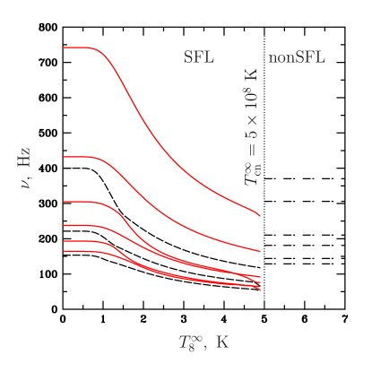
Figure 7: Spectrum of quadrupolar ($l=2$) g-modes versus $T_{8}^{\infty}\equiv T^{\infty}/(10^{8}\,\rm K)$. Critical temperatures: $T_{\rm cn}^{\infty}=5\times 10^{8}~{}\rm K$, $T_{\rm cp}^{\infty}=3\times 10^{9}~{}\rm K$. $\rm\Lambda$–hyperons are assumed to be non-superfluid. Solid lines: eigenfrequencies (in Hz) for the g-modes which are ‘$\rm\Lambda$–hyperonic’ at $T^{\infty}=0$. Dashed lines: eigenfrequencies for the g-modes which are ‘muonic’ at $T^{\infty}=0$. Dot–dashed lines: eigenfrequencies for the g-modes in a non-superfluid HS. Vertical dotted line: the redshifted critical temperature for neutrons.

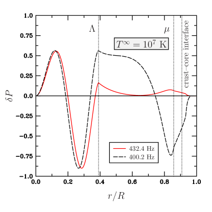
Figure 8: Perturbation of the pressure $\delta P$ (dimensionless) versus $r$ (in units of $R$) for the second ‘$\rm\Lambda$–hyperonic’ g-mode ($\nu\approx 432~{}\rm Hz$, solid line) and the first ‘muonic’ g-mode ($\nu\approx 400~{}\rm Hz$, dashed line). The red-shifted internal temperature is chosen to be $T^{\infty}=10^{7}~{}\rm K$. Vertical dotted lines: the threshold for the appearance of muons and $\rm\Lambda$–hyperons.

6 Summary

In this paper we generalized to the case of the nucleon-hyperon matter an approximate method of decoupling of superfluid and normal degrees of freedom, suggested by Gusakov & Kantor (2011) and Gusakov et al. (2013). We showed that the equations governing the oscillations of superfluid hyperon stars (HSs) can be split into two weakly coupled systems of equations with the coupling parameters $s_{\rm e}$, $s_{\rm\mu}$, and $s_{\rm str}$, given by Eq. (50). These two systems describe the ‘normal’ and ‘superfluid’ oscillation modes. Neglecting the rather small coupling terms (i.e. putting $s_{\rm e}=s_{\rm\mu}=s_{\rm str}=0$; the so called ‘decoupling approximation’) allows one to drastically simplify the calculations of the oscillation spectra. Namely, we have shown that in the decoupling regime the normal modes coincide with the ordinary modes of a non-superfluid HS and can be calculated within the non-superfluid hydrodynamics. As for the superfluid modes, in this approximation they can be calculated by using only two ‘superfluid’ equations (54) and (55) (along with the continuity equations (16) and the conditions $\delta U_{({\rm b})}^{\alpha}=\delta g^{\alpha\beta}=0$). These modes do not perturb metric, pressure, baryon current density, and are localized in the superfluid region of a star. It is shown how the proposed approach can be modified to study the oscillations in rotating HSs, containing arrays of Feynman-Onsager vortices.

An efficiency of the presented decoupling scheme is illustrated in Section 4 by the calculation, using modern hyperonic EOSs, of the sound speeds in the superfluid nucleon-hyperon matter at arbitrary temperature. It is shown that the approximate approach qualitatively well reproduces the results of the accurate calculation. Summarizing, the decoupling scheme presented here can be used to study various oscillation modes in rotating superfluid HSs (e.g., p-, f-, and r-modes). Such a detailed analysis is beyond the scope of the present paper.

Unfortunately, there exist a class of oscillations, namely the gravity modes (g-modes), that cannot be treated within the proposed simple scheme and should be considered separately. We have performed such an analysis in Section 5, where we, for the first time, discussed the composition g-modes in a star with a superfluid $\rm npe\mu\Lambda$ core. Our consideration complements the results of Kantor & Gusakov (2014) who analysed the g-modes in superfluid neutron stars with an $\rm npe\mu$ core. We showed that such a HS harbours two types of superfluid g-modes, which we call ‘muonic’ and ‘$\rm\Lambda$–hyperonic’. The eigenfrequencies of g-modes in superfluid HSs turn out to be exceptionally large (up to $\nu\approx 742~{}{\rm Hz}$ for the considered HS model). This may have a strong impact on the properties of inertial-gravity modes in rotating stars, and, as a consequence, on damping and saturation of r-modes with which they can interact. Also, the g-modes analysed in this paper may substantially modify gravitational-wave signal from coalescing HS–compact star (or HS–black hole) binaries (see Lai 1999; Ho & Lai 1999). More details on these issues as well as other possible implications of our result are discussed by Kantor & Gusakov (2014). We hope to address some of these problems in the near future.

7 Acknowledgements

We are very grateful to D.P. Barsukov, E.M. Kantor, and D.G. Yakovlev for reading the draft of the paper and many valuable suggestions, and to A.I. Chugunov for discussions. This work was partially supported by RFBR (grants 14-02-00868-a and 14-02-31616-mol-a), by RF president programme (grants MK-506.2014.2 and NSh-294.2014.2), and by the Dynasty Foundation.

Appendix A Error estimates for superfluid modes in the decoupling approximation

As mentioned in Section 3.3, if all the coupling parameters are strictly zero ($s_{\rm e}=s_{\rm\mu}=s_{\rm str}=0$), then the superfluid oscillation modes can be studied by making use of the potentiality conditions for motion of superfluid components (24) together with the continuity equations (16) and the conditions $\delta U_{({\rm b})}^{\alpha}=\delta g^{\alpha\beta}=0$.

However, if the coupling parameters are finite (but small), which is the case for realistic EOSs, then the application of the decoupling approximation scheme directly to equation (24) will lead to significant errors and hence is not appropriate. In this section we briefly explain this fact and demonstrate that use of ‘superfluid’ equations (54) and (55) instead of (24) substantially reduce errors and thus is more suitable for calculations of superfluid modes in the decoupling approximation.

Suppose that we have calculated some superfluid oscillation modes in the decoupling regime, assuming $\delta U_{({\rm b})}^{\alpha}=\delta g^{\alpha\beta}=0$. How good is this approximation if the coupling parameters are small but finite? To estimate an error one has to compare the various terms depending on the baryon four-velocity perturbation $\delta U_{({\rm b})}^{\alpha}$ and on the superfluid vectors $w_{(i)}^{\alpha}$. Since in the fully decoupled case $\delta U_{({\rm b})}^{\alpha}$ vanishes for the superfluid modes, it should be small, $\sim O(|s_{\rm e}|+|s_{\mu}|+|s_{\rm str}|)$, in the exact calculation. In other words, for the superfluid modes one can make the following estimate, $\delta U_{({\rm b})}\sim sW$, where $s=|s_{\rm e}|+|s_{\rm\mu}|+|s_{\rm str}|$, and $\delta U_{({\rm b})}$ and $W$ are the absolute values of the perturbations of the baryon four-velocity $\delta U_{({\rm b})}^{\alpha}$ and the superfluid four-vector $W^{\alpha}=\sum_{i}Y_{ik}w_{(k)}^{\alpha}$, respectively: $\delta U_{({\rm b})}\equiv\sqrt{|\delta U_{({\rm b})}^{\alpha}\delta U_{({\rm b})\alpha}|}$, $W\equiv 1/n_{\rm b}\sqrt{|W^{\alpha}W_{\alpha}|}$.

First, we show that the use of the potentiality conditions (24) leads to large errors if calculations are made in the fully decoupled case ($s=0$). Let us consider a harmonic perturbation ($\propto{\rm e}^{{\rm i}\omega t}$) of a non-rotating star, assuming, for simplicity, that only $\rm\Lambda$–hyperons are superfluid. Equation (24) for $\rm\Lambda$–hyperons in the linear approximation reads (we take $\beta=0$ and $\alpha=1,2,3$)

$${\rm i}\omega\left(w_{({\rm\Lambda})\alpha}+\mu_{\rm\Lambda}\delta u_{\alpha}\right)-\frac{\partial}{\partial x^{\alpha}}\left(u_{0}\delta\mu_{\Lambda}\right)=0.$$ (89)

Using the definitions for $U_{({\rm b})\alpha}$ (15) and $W_{\alpha}$, one can rewrite equation (89) as

$${\rm i}\omega\left[\frac{n_{\rm b}}{Y_{\Lambda\Lambda}}W_{\alpha}+\mu_{\Lambda}\left(\delta U_{({\rm b})\alpha}-W_{\alpha}\right)\right]=\frac{\partial}{\partial x^{\alpha}}\left(u_{0}\delta\mu_{\Lambda}\right).$$ (90)

In the left-hand side of equation (90) the ‘superfluid’ terms, depending on $W_{\alpha}$, are much greater than the ‘normal’ terms, depending on $\delta U_{({\rm b})\alpha}$, because $\delta U_{({\rm b})}\sim sW$. The approximation $\delta U_{({\rm b})\alpha}=0$ is valid only if the same is true also for the terms in the right-hand side of this equation, namely for the quantity $\delta\mu_{\rm\Lambda}$. Generally, $\delta\mu_{\Lambda}$ depends on both the baryon velocity $\delta U_{({\rm b})\alpha}$ and superfluid four-vector $W_{\alpha}$. Let us express $\delta\mu_{\rm\Lambda}$ through the number density perturbations $\delta n_{\rm b}$, $\delta n_{\rm e}$, $\delta n_{\rm\mu}$, and $\delta n_{\rm str}$:

$$\delta\mu_{\rm\Lambda}=\frac{\delta n_{\rm b}}{n_{\rm b}}\frac{\partial\mu_{\Lambda}}{\partial\ln n_{\rm b}}+\frac{\delta n_{\rm e}}{n_{\rm e}}\frac{\partial\mu_{\Lambda}}{\partial\ln n_{\rm e}}+\frac{\delta n_{\rm\mu}}{n_{\rm\mu}}\frac{\partial\mu_{\Lambda}}{\partial\ln n_{\rm\mu}}+\frac{\delta n_{\rm str}}{n_{\rm str}}\frac{\partial\mu_{\Lambda}}{\partial\ln n_{\rm str}}.$$ (91)

These perturbations can in turn be expressed through $\delta U_{({\rm b})}^{\alpha}$ and $W^{\alpha}$ using the continuity equations (15) and (16):

$$\frac{\delta n_{\rm b}}{n_{\rm b}}=-\frac{1}{{\rm i}\omega}{\rm e}^{\nu/2}\left({\delta U_{({\rm b})}^{\alpha}}\phantom{}_{;\alpha}+\frac{{\rm d}\ln n_{\rm b}}{{\rm d}r}\delta U_{({\rm b})}^{r}\right),$$ (92)

$$\frac{\delta n_{\rm e}}{n_{\rm e}}=-\frac{1}{{\rm i}\omega}{\rm e}^{\nu/2}\left[{\left(\delta U_{({\rm b})}^{\alpha}-W^{\alpha}\right)}\phantom{}_{;\alpha}+\frac{{\rm d}\ln n_{\rm e}}{{\rm d}r}\left(\delta U_{({\rm b})}^{r}-W^{r}\right)\right],$$ (93)

$$\frac{\delta n_{\rm\mu}}{n_{\rm\mu}}=-\frac{1}{{\rm i}\omega}{\rm e}^{\nu/2}\left[{\left(\delta U_{({\rm b})}^{\alpha}-W^{\alpha}\right)}\phantom{}_{;\alpha}+\frac{{\rm d}\ln n_{\rm\mu}}{{\rm d}r}\left(\delta U_{({\rm b})}^{r}-W^{r}\right)\right],$$ (94)

$$\frac{\delta n_{{\rm str}}}{n_{{\rm str}}}=-\frac{1}{{\rm i}\omega}{\rm e}^{\nu/2}\left[{\left(\delta U_{({\rm b})}^{\alpha}+\frac{n_{\rm b}-n_{{\rm str}}}{n_{{\rm str}}}W^{\alpha}\right)}\phantom{}_{;\alpha}+\frac{{\rm d}\ln n_{{\rm str}}}{{\rm d}r}\left(\delta U_{({\rm b})}^{r}+\frac{n_{\rm b}-n_{{\rm str}}}{n_{{\rm str}}}W^{r}\right)\right].$$ (95)

After substituting (92)–(95) into (91), one can roughly estimate the ratio of normal to superfluid terms in $\delta\mu_{\rm\Lambda}$ as

$$\frac{\text{normal~{}terms~{}in~{}}\delta\mu_{\rm\Lambda}}{\text{SFL~{}terms~{}in~{}}\delta\mu_{\rm\Lambda}}\sim z\frac{\delta U_{({\rm b})}}{W}\sim zs$$ (96)

(remember that $\delta U_{({\rm b})}\sim sW$), where

$$z=-\left(\frac{\partial\mu_{\rm\Lambda}}{\partial\ln n_{\rm b}}+\frac{\partial\mu_{\rm\Lambda}}{\partial\ln n_{\rm e}}+\frac{\partial\mu_{\rm\Lambda}}{\partial\ln n_{\rm\mu}}+\frac{\partial\mu_{\rm\Lambda}}{\partial\ln n_{\rm str}}\right)/\left(\frac{\partial\mu_{\rm\Lambda}}{\partial\ln n_{\rm e}}+\frac{\partial\mu_{\rm\Lambda}}{\partial\ln n_{\rm\mu}}+\frac{\partial\mu_{\rm\Lambda}}{\partial\ln n_{\rm str}}\frac{n_{\rm str}-n_{\rm b}}{n_{\rm str}}\right).$$ (97)

For the EOSs GM1A, GM1’B, and TM1C $zs$ can be larger than unity even when $s$ is small. For example, for the EOS TM1C $z\approx 14.6$ and $|z||s|\approx 1.66$ at $n_{\rm b}=0.5~{}{\rm fm}^{-3}$ . Thus, for superfluid modes the terms depending on $\delta U_{({\rm b})}^{\alpha}$ can be even greater than the terms depending on $W^{\alpha}$. This means that the approximation $\delta U_{({\rm b})}^{\alpha}=0$ leads to completely wrong results if we use it together with the potentiality conditions (24).

Now let us check whether the approximation $\delta U_{({\rm b})}^{\alpha}=0$ is suitable for calculating the superfluid modes within the approach presented in Section 3, when we use equation (55) instead of equation (89). We have to compare the ‘normal’ and ‘superfluid’ terms entering the expressions for $\Delta\mu_{j}$, where $j={\rm e}$, ${\rm\mu}$, ${\rm\Lambda}$. One can write out an expansion for $\Delta\mu_{j}$ similar to equation (91),

$$\Delta\mu_{j}=\frac{\delta n_{\rm b}}{n_{\rm b}}\frac{\partial\Delta\mu_{j}}{\partial\ln n_{\rm b}}+\frac{\delta n_{\rm e}}{n_{\rm e}}\frac{\partial\Delta\mu_{j}}{\partial\ln n_{\rm e}}+\frac{\delta n_{\rm\mu}}{n_{\rm\mu}}\frac{\partial\Delta\mu_{j}}{\partial\ln n_{\rm\mu}}+\frac{\delta n_{\rm str}}{n_{\rm str}}\frac{\partial\Delta\mu_{j}}{\partial\ln n_{\rm str}}.$$ (98)

Using then equations (92)–(95), one can estimate the ratio of the ‘normal’ to ‘superfluid’ terms in $\Delta\mu_{j}$ as

$$\frac{\text{normal~{}terms~{}in~{}}\Delta\mu_{j}}{\text{SFL~{}terms~{}in~{}}\Delta\mu_{j}}\sim z_{j}\frac{\delta U_{({\rm b})}}{W}\sim z_{j}s,$$ (99)

where

$$z_{j}=-\left(\frac{\partial\Delta\mu_{j}}{\partial\ln n_{\rm b}}+\frac{\partial\Delta\mu_{j}}{\partial\ln n_{\rm e}}+\frac{\partial\Delta\mu_{j}}{\partial\ln n_{\rm\mu}}+\frac{\partial\Delta\mu_{j}}{\partial\ln n_{\rm str}}\right)/\left(\frac{\partial\Delta\mu_{j}}{\partial\ln n_{\rm e}}+\frac{\partial\Delta\mu_{j}}{\partial\ln n_{\rm\mu}}+\frac{\partial\Delta\mu_{j}}{\partial\ln n_{\rm str}}\frac{n_{\rm str}-n_{\rm b}}{n_{\rm str}}\right).$$ (100)

As a result, the total error of the approximation $\delta U_{({\rm b})}^{\alpha}=0$ in equation (55) can be estimated as $(|z_{\rm e}|+|z_{\rm\mu}|+|z_{\rm\Lambda}|)|s|$, which is the sum of errors arising from the three terms in the right-hand side of that equation. For the hyperonic EOSs GM1A, GM1’B, and TM1C $|z_{\rm e}|,|z_{\rm\mu}|,|z_{\rm\Lambda}|\sim 1$, whereas the coupling parameters $|s_{\rm e}|,|s_{\rm\mu}|,|s_{\rm str}|\ll 1$, so our perturbative scheme is valid. For example, for the EOS TM1C at $n_{\rm b}=0.5~{}{\rm fm}^{-3}$ $(|z_{\rm e}|+|z_{\rm\mu}|+|z_{\rm\Lambda}|)|s|\approx 0.23$, hence our decoupling scheme developed in Section 3 calculates the superfluid modes within the accuracy of $\sim 20\%$. Estimates presented here are supported by calculations of sound speeds in Section 4.

Appendix B Superfluid oscillation equations for different sets of superfluid particle species

In Section 3.3 we derived the superfluid equation (52) using the potentiality condition (24) for the neutron superfluid four-vector $w_{({\rm n})}^{\alpha}$ as well as the energy-momentum conservation law (22). In addition, we used the fact that $P+\varepsilon-\mu_{\rm n}n_{\rm b}$ and $\partial_{\beta}P-n_{\rm b}\partial_{\beta}\mu_{\rm n}$ are small quantities, vanishing in equilibrium. The same derivation can be performed for any baryon species $i$, if the following two conditions are fulfilled:

1. the superfluid four-vector $w_{(i)\alpha}$ satisfies the potentiality equation ${\left(w_{(i)\alpha}+\mu_{i}u_{\alpha}\right)}\phantom{}_{;\beta}-{\left(w_{(i)\beta}+\mu_{i}u_{\beta}\right)}\phantom{}_{;\alpha}=0$;

2. the difference of chemical potentials $\mu_{i}-\mu_{\rm n}$ is a small quantity, vanishing in equilibrium.

These conditions are fulfilled e.g., for $\rm\Lambda$– or ${\rm\Xi}^{0}$–hyperons.

Furthermore, one can take not only a single superfluid four-vector $w_{(i)\alpha}$ and chemical potential $\mu_{i}$, but also an appropriate linear combination of $w_{(i)\alpha}$ and the corresponding linear combination of $\mu_{i}$. For example, if we introduce a ‘quasiparticle’ $({\rm p}+{\rm\Sigma}^{-})/2$, with $w_{\alpha}=(w_{({\rm p})\alpha}+w_{({\rm\Sigma}^{-})\alpha})/2$ and the chemical potential $\mu=(\mu_{\rm p}+\mu_{{\rm\Sigma}^{-}})/2$, then it meets the conditions (i) and (ii). Therefore, even in this case we can derive a superfluid equation for this ‘quasiparticle’.

Let us demonstrate this for an arbitrary particle (or ‘quasiparticle’) $A$, which meets the conditions (i) and (ii) [in particular, $\mu_{A}-\mu_{\rm n}$ vanishes in equilibrium]. The derivation is the same as that for equations (52)–(55). Now we shall outline it, underlining, for clarity, the additional terms that have not appeared in the derivation of (52)–(55). Using the energy-momentum conservation law (22) together with the potentiality condition (24) for (quasi)particle $A$, one obtains an equation similar to (51),

$${{T_{\alpha}}^{\beta}}\phantom{}_{;\beta}+u_{\alpha}u_{\gamma}{T^{\gamma\beta}}\phantom{}_{;\beta}-n_{\rm b}u^{\beta}\left[{\left(w_{(A)\alpha}+\mu_{A}u_{\alpha}\right)}\phantom{}_{;\beta}-{\left(w_{(A)\beta}+\mu_{A}u_{\beta}\right)}\phantom{}_{;\alpha}\right]\\ =(P+\varepsilon-\mu_{A}n_{\rm b})u^{\beta}{u_{\alpha}}\phantom{}_{;\beta}+\left({P}\phantom{}_{;\beta}-n_{\rm b}{\mu_{A}}\phantom{}_{;\beta}\right)u_{\alpha}u^{\beta}+\left({P}\phantom{}_{;\alpha}-n_{\rm b}{\mu_{A}}\phantom{}_{;\alpha}\right)\\ +(g_{\alpha\gamma}+u_{\alpha}u_{\gamma})u^{\beta}{(\mu_{\rm n}n_{\rm b}W^{\gamma})}\phantom{}_{;\beta}+\mu_{\rm n}n_{\rm b}\left({{u^{\beta}}}\phantom{}_{;\beta}W_{\alpha}+{u_{\alpha}}\phantom{}_{;\beta}W^{\beta}\right)-n_{\rm b}u^{\beta}\left[{w_{(A)\alpha}}\phantom{}_{;\beta}-{w_{(A)\beta}}\phantom{}_{;\alpha}\right]=0.$$ (101)

It follows from equations (31) and (33) that

$$P+\varepsilon-\mu_{A}n_{\rm b}=-\Delta\mu_{\rm e}n_{\rm e}-\Delta\mu_{\rm\mu}n_{\rm\mu}-\Delta\mu_{\rm\Lambda}n_{\rm str}+\underline{\Delta\mu_{A}n_{\rm b}},\quad\Delta\mu_{A}\equiv\mu_{\rm n}-\mu_{A},$$ (102)

$${\rm d}P-n_{\rm b}{\rm d}\mu_{A}=-n_{\rm e}{\rm d}\Delta\mu_{\rm e}-n_{\rm\mu}{\rm d}\Delta\mu_{\rm\mu}-n_{\rm str}{\rm d}\Delta\mu_{\rm\Lambda}+\underline{n_{\rm b}{\rm d}\Delta\mu_{A}}.$$ (103)

Using these relations one can rewrite equation (101) as

$$\left(-\Delta\mu_{\rm e}n_{\rm e}-\Delta\mu_{\rm\mu}n_{\rm\mu}-\Delta\mu_{\rm\Lambda}n_{\rm str}+\underline{\Delta\mu_{A}n_{\rm b}}\right)u^{\beta}{u_{\alpha}}\phantom{}_{;\beta}+\left(-n_{\rm e}\partial_{\beta}{\Delta\mu_{\rm e}}-n_{\rm\mu}\partial_{\beta}{\Delta\mu_{\rm\mu}}-n_{\rm str}\partial_{\beta}{\Delta\mu_{\rm\Lambda}}+\underline{n_{\rm b}\partial_{\beta}\Delta\mu_{A}}\right)u_{\alpha}u^{\beta}\\ +\left(-n_{\rm e}\partial_{\alpha}{\Delta\mu_{\rm e}}-n_{\rm\mu}\partial_{\alpha}{\Delta\mu_{\rm\mu}}-n_{\rm str}\partial_{\alpha}{\Delta\mu_{\rm\Lambda}}+\underline{n_{\rm b}\partial_{\alpha}\Delta\mu_{A}}\right)+(g_{\alpha\gamma}+u_{\alpha}u_{\gamma})u^{\beta}{(\mu_{\rm n}n_{\rm b}W^{\gamma})}\phantom{}_{;\beta}+\mu_{\rm n}n_{\rm b}\left({{u^{\beta}}}\phantom{}_{;\beta}W_{\alpha}+{u_{\alpha}}\phantom{}_{;\beta}W^{\beta}\right)\\ -n_{\rm b}u^{\beta}\left[{w_{(A)\alpha}}\phantom{}_{;\beta}-{w_{(A)\beta}}\phantom{}_{;\alpha}\right]=0.$$ (104)

In the case of a non-rotating star with the Schwarzschild metric, when all perturbations depend on time as ${\rm e}^{{\rm i}\omega t}$, the spatial components ($\alpha=1,2,3$) of this equation take the following final form:

$${\rm i}\omega n_{\rm b}(\mu_{\rm n}W_{\alpha}-w_{(A)\alpha})=n_{\rm e}\frac{\partial}{\partial x^{\alpha}}\left(\Delta\mu_{\rm e}{\rm e}^{\nu/2}\right)+n_{\rm\mu}\frac{\partial}{\partial x^{\alpha}}\left(\Delta\mu_{\rm\mu}{\rm e}^{\nu/2}\right)+n_{\rm str}\frac{\partial}{\partial x^{\alpha}}\left(\Delta\mu_{\rm\Lambda}{\rm e}^{\nu/2}\right)-\underline{n_{\rm b}\frac{\partial}{\partial x^{\alpha}}\left(\Delta\mu_{A}{\rm e}^{\nu/2}\right)},\quad\alpha=1,2,3.$$ (105)

Now let us focus on the following question. In a real neutron star, depending on a density and temperature, some particle species are superfluid, some are present but non-superfluid, while others are absent. How many different equations do we need to cover all the cases? It turns out that, if the thresholds for the appearance of hyperons $n_{({\rm b})}^{(i)}$ satisfy the inequality $n_{({\rm b})}^{({\rm\Lambda})}<n_{({\rm b})}^{({\rm\Xi}^{-})}<n_{({\rm b})}^{({\rm\Xi}^{0})}<n_{({\rm b})}^{({\rm\Sigma}^{-})}$ (which is true for many modern equations of state, including GM1A, GM1‘B, and TM1C), then in all the situations there are no more than two superfluid degrees of freedom. Interestingly, all the cases except one (see below) can be covered with the only four choices of (quasi)particle $A$ in equation (104) (or 105),

1. $A={\rm n}$

2. $A={\rm\Lambda}$

3. $A={\rm\Xi}^{0}$

4. $A=({\rm p}+{\rm\Sigma}^{-})/2$.

The special case is when ${\rm\Xi}^{-}$– and ${\rm\Sigma}^{-}$–hyperons are the only superfluid species in the system. Then we can construct superfluid equation by subtracting the potentiality condition (24) for ${\rm\Sigma}^{-}$–hyperons from the potentiality condition for ${\rm\Xi}^{-}$– hyperons. Using then the fact that $\mu_{{\rm\Sigma}^{-}}-\mu_{{\rm\Xi}^{-}}=\mu_{\rm n}-\mu_{\rm\Lambda}=\Delta\mu_{\rm\Lambda}$ (see equations 7–9), one gets

$${\rm i}\omega(w_{({\rm\Xi}^{-})\alpha}-w_{({\rm\Sigma}^{-})\alpha})=\frac{\partial}{\partial x^{\alpha}}\left(\Delta\mu_{\rm\Lambda}{\rm e}^{\nu/2}\right),\quad\alpha=1,2,3.$$ (106)

Let us illustrate the above statements by considering a few possible situations.

(1) Assume that the protons as well as the ${\rm\Xi}^{0}$– and ${\rm\Xi}^{-}$–hyperons are superfluid, while other particles are not. Then there are two superfluid degrees of freedom; the use of the superfluid four-vector $w_{({\rm n})\alpha}$ and, as a consequence, of the superfluid equation for neutrons, seems to be incorrect (neutrons are normal!). However, one can formally introduce a variable $w_{({\rm n})\alpha}\equiv w_{({\rm p})\alpha}+w_{({\rm\Xi}^{-})\alpha}-w_{({\rm\Xi}^{0})\alpha}$, such that the superfluid equation for ‘neutrons’ remains valid (remember that $\mu_{\rm n}=\mu_{\rm p}+\mu_{{\rm\Xi}^{-}}-\mu_{{\rm\Xi}^{0}}$). Moreover, proceeding in the same way, one can introduce a variable $w_{({\rm\Lambda})\alpha}\equiv(w_{({\rm p})\alpha}+w_{({\rm\Xi}^{-})\alpha})/2$, and use the standard superfluid equation for ‘$\rm\Lambda$–hyperons’ (55). As a result, we cover this case by formally introducing superfluid ‘quasiparticles’ ${\rm n}={\rm p}+{\rm\Xi}^{-}-{\rm\Xi}^{0}$ (case i) and ${\rm\Lambda}=({\rm p}+{\rm\Xi}^{-})/2$ (case ii).

(2) Assume now that only the neutrons, protons, and ${\rm\Sigma}^{-}$–hyperons are superfluid. In this situation one also has two superfluid degrees of freedom and, therefore, two superfluid equations. The first is the equation for neutrons (case i), while the second is the superfluid equation for a quasiparticle $A=({\rm p}+{\rm\Sigma}^{-})/2$ (case iv).

References

- Andersson (2003) Andersson N., 2003, Classical and Quantum Gravity, 20, 105
- Andersson & Comer (2001) Andersson N., Comer G. L., 2001, MNRAS, 328, 1129
- Andersson et al. (2011) Andersson N., Ferrari V., Jones D. I., Kokkotas K. D., Krishnan B., Read J. S., Rezzolla L., Zink B., 2011, General Relativity and Gravitation, 43, 409
- Andersson et al. (2013) Andersson N., et al., 2013, Classical and Quantum Gravity, 30, 193002
- Andersson et al. (2014) Andersson N., Jones D. I., Ho W. C. G., 2014, MNRAS, 442, 1786
- Bednarek et al. (2012) Bednarek I., Haensel P., Zdunik J. L., Bejger M., Mańka R., 2012, A&A, 543, A157
- Benhar et al. (2004) Benhar O., Ferrari V., Gualtieri L., 2004, Phys. Rev. D, 70, 124015
- Blázquez-Salcedo et al. (2014) Blázquez-Salcedo J. L., González-Romero L. M., Navarro-Lérida F., 2014, Phys. Rev. D, 89, 044006
- Bondarescu et al. (2007) Bondarescu R., Teukolsky S. A., Wasserman I., 2007, Phys. Rev. D, 76, 064019
- Chirenti et al. (2015) Chirenti C., de Souza G. H., Kastaun W., 2015, Phys. Rev. D, 91, 044034
- Chugunov & Gusakov (2011) Chugunov A. I., Gusakov M. E., 2011, MNRAS, 418, L54
- Cowling (1941) Cowling T. G., 1941, MNRAS, 101, 367
- Finn (1987) Finn L. S., 1987, MNRAS, 227, 265
- Gaertig & Kokkotas (2009) Gaertig E., Kokkotas K. D., 2009, Phys. Rev. D, 80, 064026
- Gezerlis et al. (2014) Gezerlis A., Pethick C. J., Schwenk A., 2014, preprint, (arXiv:1406.6109)
- Gualtieri et al. (2014) Gualtieri L., Kantor E. M., Gusakov M. E., Chugunov A. I., 2014, Phys. Rev. D, 90, 024010
- Gusakov (2007) Gusakov M. E., 2007, Phys. Rev. D, 76, 083001
- Gusakov & Andersson (2006) Gusakov M. E., Andersson N., 2006, MNRAS, 372, 1776
- Gusakov & Kantor (2008) Gusakov M. E., Kantor E. M., 2008, Phys. Rev. D, 78, 083006
- Gusakov & Kantor (2011) Gusakov M. E., Kantor E. M., 2011, Phys. Rev. D, 83, 081304
- Gusakov et al. (2009a) Gusakov M. E., Kantor E. M., Haensel P., 2009a, Phys. Rev. C, 79, 055806
- Gusakov et al. (2009b) Gusakov M. E., Kantor E. M., Haensel P., 2009b, Phys. Rev. C, 80, 015803
- Gusakov et al. (2013) Gusakov M. E., Kantor E. M., Chugunov A. I., Gualtieri L., 2013, MNRAS, 428, 1518
- Gusakov et al. (2014) Gusakov M. E., Haensel P., Kantor E. M., 2014, MNRAS, 439, 318
- Haensel et al. (2002) Haensel P., Levenfish K. P., Yakovlev D. G., 2002, A&A, 394, 213
- Haskell & Andersson (2010) Haskell B., Andersson N., 2010, MNRAS, 408, 1897
- Haskell et al. (2012) Haskell B., Andersson N., Comer G. L., 2012, Phys. Rev. D, 86, 063002
- Ho & Lai (1999) Ho W. C. G., Lai D., 1999, MNRAS, 308, 153
- Israel et al. (2005) Israel G. L., et al., 2005, ApJ, 628, L53
- Kantor & Gusakov (2009) Kantor E. M., Gusakov M. E., 2009, Phys. Rev. D, 79, 043004
- Kantor & Gusakov (2011) Kantor E. M., Gusakov M. E., 2011, Phys. Rev. D, 83, 103008
- Kantor & Gusakov (2012) Kantor E. M., Gusakov M. E., 2012, in Lewandowski W., Maron O., Kijak J., eds, Astronomical Society of the Pacific Conference Series Vol. 466, Electromagnetic Radiation from Pulsars and Magnetars. p. 211
- Kantor & Gusakov (2014) Kantor E. M., Gusakov M. E., 2014, MNRAS, 442, L90
- Khalatnikov & Bekarevich (1961) Khalatnikov I. M., Bekarevich I. L., 1961, JETP, 40, 920
- Lai (1999) Lai D., 1999, MNRAS, 307, 1001
- Landau & Lifshitz (1980) Landau L. D., Lifshitz E. M., 1980, Statistical physics. Pt.1, Pt.2
- Lee (1995) Lee U., 1995, A&A, 303, 515
- Lee (2014) Lee U., 2014, MNRAS, 442, 3037
- Lindblom & Owen (2002) Lindblom L., Owen B. J., 2002, Phys. Rev. D, 65, 063006
- Lindblom & Splinter (1990) Lindblom L., Splinter R. J., 1990, ApJ, 348, 198
- Lombardo & Schulze (2001) Lombardo U., Schulze H.-J., 2001, in Blaschke D., Glendenning N. K., Sedrakian A., eds, Lecture Notes in Physics, Berlin Springer Verlag Vol. 578, Physics of Neutron Star Interiors. p. 30 (arXiv:astro-ph/0012209)
- McDermott et al. (1983) McDermott P. N., van Horn H. M., Scholl J. F., 1983, ApJ, 268, 837
- Mendell & Lindblom (1991) Mendell G., Lindblom L., 1991, Annals of Physics, 205, 110
- Nayyar & Owen (2006) Nayyar M., Owen B. J., 2006, Phys. Rev. D, 73, 084001
- Page et al. (2013) Page D., Lattimer J. M., Prakash M., Steiner A. W., 2013, preprint, (arXiv:1302.6626)
- Passamonti et al. (2015) Passamonti A., Andersson N., Ho W. C. G., 2015, preprint, (arXiv:1504.07470)
- Potekhin et al. (2013) Potekhin A. Y., Fantina A. F., Chamel N., Pearson J. M., Goriely S., 2013, A&A, 560, A48
- Prix & Rieutord (2002) Prix R., Rieutord M., 2002, A&A, 393, 949
- Reisenegger & Goldreich (1992) Reisenegger A., Goldreich P., 1992, ApJ, 395, 240
- Sathyaprakash et al. (2012) Sathyaprakash B., et al., 2012, Classical and Quantum Gravity, 29, 124013
- Strohmayer & Mahmoodifar (2014a) Strohmayer T., Mahmoodifar S., 2014a, ApJ, 784, 72
- Strohmayer & Mahmoodifar (2014b) Strohmayer T., Mahmoodifar S., 2014b, ApJ, 793, L38
- Strohmayer & Watts (2006) Strohmayer T. E., Watts A. L., 2006, ApJ, 653, 593
- Takatsuka et al. (2006) Takatsuka T., Nishizaki S., Yamamoto Y., Tamagaki R., 2006, Progress of Theoretical Physics, 115, 355
- Wang & Shen (2010) Wang Y. N., Shen H., 2010, Phys. Rev. C, 81, 025801
- Watts & Strohmayer (2007a) Watts A. L., Strohmayer T. E., 2007a, Advances in Space Research, 40, 1446
- Watts & Strohmayer (2007b) Watts A. L., Strohmayer T. E., 2007b, Ap&SS, 308, 625
- Weissenborn et al. (2012a) Weissenborn S., Chatterjee D., Schaffner-Bielich J., 2012a, Phys. Rev. C, 85, 065802
- Weissenborn et al. (2012b) Weissenborn S., Chatterjee D., Schaffner-Bielich J., 2012b, Nuclear Physics A, 881, 62
- Yakovlev et al. (1999) Yakovlev D. G., Levenfish K. P., Shibanov Y. A., 1999, Soviet Physics Uspekhi, 42, 737