Coupling spin to velocity: collective motion of Hamiltonian polar particles

Abstract

We propose a conservative two-dimensional particle model in which particles carry a continuous and classical spin. The model includes standard ferromagnetic interactions between spins of two different particles, and a nonstandard coupling between spin and velocity of the same particle inspired by the coupling observed in self-propelled hard discs. Because of this coupling Galilean invariance is broken and the conserved linear momentum associated to translation invariance is not proportional to the velocity of the center of mass. Also, the dynamics is not invariant under a global rotation of the spins alone. This, in principle, leaves room for collective motion and thus raises the question whether collective motion can arise in Hamiltonian systems. We study the statistical mechanics of such a system, and show that, in the fully connected (or mean-field) case, a transition to collective motion does exist in spite of momentum conservation. Interestingly, the velocity of the center of mass, which in the absence of Galilean invariance, is a relevant variable, also feeds back on the magnetization properties, as it acts as an external magnetic field that smoothens the transition. Molecular dynamics simulations of finite size systems indeed reveal a rich phase diagram, with a transition from a disordered to a homogeneous polar phase, but also more complex inhomogeneous phases with local order interrupted by topological defects.

Keywords Collective motion, XY-model, Hamiltonian dynamics, Statistical mechanics, Numerical simulations

1 Introduction

Spontaneous collective motion, a coordinated motion of an assembly of moving entities which interact locally without any leader, has recently drawn a lot of attention from the statistical physics community [1, 2]. Such a phenomenon is present both in biological systems like motility assays [3, 4, 5, 6] and bacterial colonies [7, 8] or on a larger scale insects swarms [9] and flocks of birds [10, 11], as well as in engineered systems like driven colloids [12, 13, 14, 15], droplets [16, 17], or grains [18, 19, 20, 21]. From a theoretical perspective, such moving individuals are represented as polar self-propelled particles, that is, particles set in motion by a driving force directed along the heading vector of the particle. This driving force being balanced by a friction force, a constant speed is reached in the absence of interaction with obstacles or other particles. Assuming, as a simplification, that the speed is always constant leads to minimal models like the Vicsek model [22], where particles also interact with their neighbors so as to align their velocity vectors, up to some noise. In other words, Vicsek-type models can be thought of as spin-models [23, 24], where particles move along the direction of their spin instead of remaining fixed on the node of a lattice. This analogy with spin models is important because in two dimensions (the dimension in which the Vicsek model is usually defined), the Mermin-Wagner theorem [25] prevents the existence of long-range order for equilibrium models of spins that are invariant under global rotation of the spins, due to the presence of low-energy excitations called spin-waves  [26, 27, 28]. The existence of long-range order in the two-dimensional Vicsek model [22, 23, 29, 30, 31] thus reveals the intrinsic non-equilibrium character of the model, and to some extent, of the phenomenon of collective motion itself. The presence of long-range order in the Vicsek model can be understood as resulting from the continuous evolution of the neighborhood of a given particle, which successively interact with different particles.

As mentioned above, an important simplification of Vicsek-type models is to identify the direction of motion with that of the heading vector of the particles. At low enough density, when the relaxation time of the velocity is short as compared to the typical time between successive interactions, this approximation is well-justified. In a denser regime however, as observed in experiments on shaken polar grains [19, 20], velocity and heading vectors may have different directions, and it is a priori relevant to consider them as distinct dynamical variables, as done in [32, 33], assuming a suitable coupling between velocity and heading. In this situation, we are thus dealing with a fluid of particles carrying a (classical) spin.

When considering both velocity and heading (or spin) variables, the possible existence of collective motion at equilibrium cannot be immediately ruled out by standard arguments if spins and velocities are coupled. The first argument (in two dimension) is the Mermin–Wagner theorem, but its applicability is not granted if spins interact with velocities, because the system is then no longer invariant under a rotation of the spins alone. The second argument is that for an isolated system at equilibrium the momentum is conserved and no spontaneous global motion can emerge. Alternatively, boundaries or a substrate may break momentum conservation, but they act as a momentum sink, also preventing collective motion. These arguments are however valid only if the standard relation ${\bf p}=m{\bf v}$ between momentum and velocity holds. Although very general, it is well-known that such a relation breaks down when the ‘potential energy’ (the potential term in the Lagrangian) depends on the velocities as is the case for charges in magnetic field. A third argument related to the second one, is that at equilibrium the center-of-mass velocity is conjugated, in a thermodynamic sense, to momentum—just like temperature is conjugated to energy—and is thus equal to that of the surrounding medium [34]. Invoking Galilean invariance, one then usually sets the center-of-mass velocity to zero. However Galilean invariance does not hold in those above situations where the potential term in the Lagrangian depends on the velocities, so that the center-of-mass velocity should be a relevant parameter in this case. A natural question is thus to investigate whether a coupling between velocity and spin variables could break the Galilean invariance, modify the standard definition of momentum, and as a result allow for the possibility of collective motion at equilibrium—equilibrium being understood in the generic sense of the statistical steady-state of a Hamiltonian system, in the absence of external forcing.

In this paper, we investigate this issue by considering a simple two-dimensional model of point-like particles carrying a spin and evolving according to a conservative dynamics coupling spin and velocity in a minimal way. The dynamics is originally defined in a Lagrangian formalism, from which a Hamiltonian formulation is derived. A non-standard expression of the momentum of each particle in terms of its velocity and spin is obtained. We study the statistical mechanics of such a system, and show that in the fully connected (or mean-field) case a transition to collective motion occurs. The velocity of the center of mass, which in the absence of Galilean invariance, is a relevant variable, also feeds back on the magnetization properties: it acts as an external magnetic field that smoothens the transition and stabilizes non trivial local minima of the free energy. Molecular dynamics (MD) simulations of finite size systems confirm the existence of a homogeneous polar phase. Increasing sizes, the system organizes into domains of collectively moving particles structured around topological defects.

2 The model

2.1 Definition

We start by considering a liquid of XY-spins in two dimensions. The Lagrangian of such a model is described by $L=L_{\text{r}}+L_{\text{s}}$ with:

$$L_{\text{r}} =\sum_{i=1}^{N}\Bigg{(}\frac{m}{2}\dot{\mathbf{r}}_{i}^{2}-\frac{1}{2}\sum_{k(\neq i)}U(r_{ik})\Bigg{)}$$ (1a)

$$L_{\text{s}} =\sum_{i=1}^{N}\Bigg{(}\frac{I}{2}\dot{\theta}_{i}^{2}+\frac{1}{2}\sum_{k(\neq i)}J(r_{ik}){\mathbf{s}_{i}}\cdot{\mathbf{s}_{k}}+{\mathbf{h}}\cdot{\mathbf{s}_{i}}\Bigg{)}$$ (1b)

where $r_{ik}\equiv|\mathbf{r}_{k}-\mathbf{r}_{i}|$, with $\mathbf{r}_{i}$, $\theta_{i}$ and $\mathbf{s}_{i}$, denoting the position, the angle and the spin of each particle respectively (the dot on top of a variable denotes time derivative). Note that the spin $\mathbf{s}_{i}$ is defined as $\mathbf{s}_{i}={\hat{\mathbf{e}}}(\theta_{i})\equiv\cos\theta_{i}\hat{\mathbf{e}}_{x}+\sin\theta_{i}\hat{\mathbf{e}}_{y}$. The other parameters appearing in the Lagrangian are the mass $m$ of the particles, their moment of inertia $I$ associated to spin rotation, the coupling $J=J_{0}j(r_{ik})$ between spins, the external field $\mathbf{h}$, and the interaction potential $U(r_{ik})$ between particles (e.g., hard sphere or Lennard-Jones potential). With the model as it stands, there is coordination of spins at low temperature. However there is no coupling between spin and particle motion, so that no collective motion can emerge. To couple the motion of the particles to the spin we add to the Lagrangian a term

$$L_{\text{sv}}=K\sum_{i=1}^{N}{\mathbf{s}}_{i}\cdot\dot{\mathbf{r}}_{i}\,,$$ (2)

where $K$ is a coupling constant between spin and velocity, which is expected to favor the alignment of the velocity of particle $i$ to its own spin $\mathbf{s}_{i}$. Apart from the fact that it should contribute to align velocities when spins align –although we shall see that the effect is really indirect and counter-intuitive– this term is motivated by the observation of such self-alignment in real systems of self-propelled grains [32] and has been identified as a key ingredient for the dynamics of self-propelled discs [33].

Leaving aside the potential term $U$, although we shall reintroduce it when moving to the molecular dynamics simulations, our starting point is thus the following dimensionless Lagrangian:

$$L=\sum_{i=1}^{N}\Bigg{(}\frac{1}{2}\dot{\mathbf{r}}_{i}^{2}+\frac{1}{2}\dot{\theta}_{i}^{2}+(K\dot{\mathbf{r}}_{i}\!+\!\mathbf{h})\cdot\mathbf{s}_{i}+\frac{1}{2}\sum_{k(\neq i)}j(r_{ik}){\mathbf{s}_{i}}\cdot{\mathbf{s}_{k}}\Bigg{)},$$ (3)

where we used the following redefinitions

$$\mathbf{r}/\sqrt{I/m}\rightarrow\mathbf{r},\quad t/\sqrt{I/J_{0}}\rightarrow t,$$ (4a)

$$\frac{K}{\sqrt{{mJ_{0}}}}\rightarrow K,\quad\frac{\mathbf{h}}{J_{0}}\rightarrow\mathbf{h},\quad L/J_{0}\rightarrow L.$$ (4b)

The parameter $K$ now controls the strength of the alignment between spin and velocity. The Euler–Lagrange equations then read

$$\ddot{\mathbf{r}}_{i} =-K\dot{\theta}_{i}\hat{\mathbf{e}}_{\perp,i}+\sum_{k(\neq i)}\frac{\partial j(r_{ik})}{\partial\mathbf{r}_{i}}\cos\theta_{ik}$$ (5a)

$$\ddot{\theta}_{i} =(K\dot{\mathbf{r}}_{i}+\mathbf{h})\cdot{\hat{\mathbf{e}}}_{\perp,i}+\sum\limits_{k(\neq i)}j(r_{ik})\sin\theta_{ik},$$ (5b)

where $\theta_{ik}=\theta_{k}-\theta_{i}$ and $\hat{\mathbf{e}}_{\perp,i}$ is a unit vector perpendicular to the spin, defined as $\hat{\mathbf{e}}_{\perp,i}=\hat{\mathbf{e}}(\theta_{i}+\frac{\pi}{2})$. Finally, we reformulate the dynamics in the Hamiltonian formalism. The momenta $\mathbf{p}_{i}$ and $\omega_{i}$ conjugate to the positions $\mathbf{r}_{i}$ and angles $\theta_{i}$ read:

$$\mathbf{p}_{i} =\frac{\partial L}{\partial\dot{\mathbf{r}}_{i}}=\dot{\mathbf{r}}_{i}+K\mathbf{s}_{i},$$ (6a)

$$\omega_{i} =\frac{\partial L}{\partial\dot{\theta}_{i}}=\dot{\theta}_{i}.$$ (6b)

The spin of the particle acts as an internal potential vector and only for $K=0$ is the momentum equal to the velocity. The Hamiltonian is obtained by the usual Legendre transform of the Lagrangian

$$H=\sum_{i=1}^{N}\left(\mathbf{p}_{i}\cdot\dot{\mathbf{r}}_{i}+\omega_{i}{\dot{\theta}}_{i}\right)-L.$$ (7)

Expressing $\dot{\mathbf{r}}_{i}$ and $\dot{\theta}_{i}$ in terms of the conjugate variables $\mathbf{p}_{i}$ and $\omega_{i}$, one finds, discarding an irrelevant constant term:

$$H=\sum_{i=1}^{N}\Bigg{(}\frac{\mathbf{p}_{i}^{2}}{2}+\frac{\omega_{i}^{2}}{2}-(K\mathbf{p}_{i}+\mathbf{h})\cdot\mathbf{s}_{i}-\frac{1}{2}\sum_{k(\neq i)}j(r_{ik}){\mathbf{s}_{i}}\cdot{\mathbf{s}_{k}}\Bigg{)}.$$ (8)

The equations of motion follow:

$$\dot{\mathbf{r}}_{i} =\frac{\partial H}{\partial\mathbf{p}_{i}}=\mathbf{p}_{i}-K\mathbf{s}_{i}$$ (9a)

$$\dot{\mathbf{p}}_{i} =-\frac{\partial H}{\partial\mathbf{r}_{i}}=\sum_{k(\neq i)}\frac{\partial j(r_{ik})}{\partial\mathbf{r}_{i}}\cos\theta_{ik}$$ (9b)

$$\dot{\theta}_{i} =\frac{\partial H}{\partial\omega_{i}}=\omega_{i}$$ (9c)

$$\dot{\omega}_{i} =-\frac{\partial H}{\partial\theta_{i}}=(K\mathbf{p}_{i}+\mathbf{h})\cdot\hat{\mathbf{e}}_{\perp,i}+\sum_{k(\neq i)}j(r_{ik})\sin\theta_{ik}.$$ (9d)

Let us note that, up to a constant the Hamiltonian can be formally written as

$$H=\sum_{i=1}^{N}\Bigg{(}\frac{\dot{\mathbf{r}}_{i}^{2}}{2}+\frac{\omega_{i}^{2}}{2}-\mathbf{h}\cdot\mathbf{s}_{i}-\frac{1}{2}\sum_{k(\neq i)}j(r_{ik}){\mathbf{s}_{i}}\cdot{\mathbf{s}_{k}}\Bigg{)}.$$ (10)

Although this is not a proper formulation in terms of the canonical variables, it shows that written in terms of kinetic and potential energy, the Hamiltonian takes a form similar to the one of a standard liquid of particles carrying an XY-spin. The subtlety hidden in this misleadingly simple formulation is that $\dot{\mathbf{r}}_{i}$ is not proportional to $\mathbf{p}_{i}$.

2.2 Continuous Symmetries

Taking advantage of the Lagrangian formulation, we apply Noether’s theorem to obtain the conserved quantities of the dynamics, associated to the continuous transformation under which the Lagrangian is invariant.

First of all, the Lagrangian is invariant under time and space translation, so that the dynamics conserves the energy $E=H$ and the generalized linear momentum $\mathbf{P}$ obtained by summing (6a) over all particles:

$$\mathbf{P}=N\mathbf{V}+K\mathbf{M},$$ (11)

where $\mathbf{V}$ is the center of mass velocity and $\mathbf{M}=\sum_{i=1}^{N}\mathbf{s}_{i}$ is the total magnetization of the system. This simple but essential formula relates the total momentum of the system to the collective motion, described by the velocity of the center of mass, and the total magnetization of the system. Although the generalized linear momentum considered here is not proportional to the velocity of the center of mass, this conservation law is in stark contrast with most two-dimensional models for collective motion, for which momentum is not conserved.

The equations of motion are not invariant under a rotation of the system (i.e., a global rotation of the position of particles), as can be seen from (3), where the scalar product is not invariant, as the spins do not rotate, and also because of the presence of the external field $\mathbf{h}$.

Finally, let us stress a significant difference with the standard XY-model [26, 27, 28]. In the present case, there is no symmetry under rotation of the spins alone. Accordingly spin waves are not slow modes of the dynamics and the Mermin-Wagner theorem (at least in its form) does not apply, opening the way for possible long-range order.

2.3 Time reversibility

Interestingly the dynamics is not time reversible. Applying the transformation $t\rightarrow-t$:

$$\mathbf{r}_{i} \rightarrow\mathbf{r}_{i},\quad\dot{\mathbf{r}}_{i}\rightarrow-\dot{\mathbf{r}}_{i},\quad\ddot{\mathbf{r}}_{i}\rightarrow\ddot{\mathbf{r}}_{i},$$ (12a)

$$\theta_{i} \rightarrow\theta_{i},\quad\dot{\theta}_{i}\rightarrow-\dot{\theta}_{i},\quad\ddot{\theta}_{i}\rightarrow\ddot{\theta}_{i}$$ (12b)

to the Euler-Lagrange equations (5), they transform into

$$\ddot{\mathbf{r}}_{i} =K\dot{\theta}_{i}\hat{\mathbf{e}}_{\perp,i}+\sum_{k(\neq i)}\frac{\partial j(r_{ik)}}{\partial\mathbf{r}_{i}}\cos\theta_{ik}$$ (13a)

$$\ddot{\theta}_{i} =(-K\dot{\mathbf{r}}_{i}+\mathbf{h})\cdot\hat{\mathbf{e}}_{\perp,i}+\sum_{k(\neq i)}j(r_{ik})\sin\theta_{ik},$$ (13b)

which differ from the original ones [Eq. (5)], unless $K=0$. Note that although the Hamiltonian is symmetric under time reversal, it does not imply time reversibility of the trajectories because $\mathbf{p}_{i}$ transforms under time reversal into $\mathbf{p}_{i}^{\prime}=-\mathbf{p}_{i}+2K\mathbf{s}_{i}$, as can also be checked directly from Eq. (9).

The invariance of the trajectories can be recovered using the more general transformation $t\to-t$ and $\mathbf{s}_{i}\to-\mathbf{s}_{i}$. In this case, one has $\mathbf{p}_{i}\to-\mathbf{p}_{i}$ and both the Hamiltonian and the trajectories are invariant. The invariance under this more general transformation can be interpreted as a generalized form of microreversibility. At a heuristic level, this suggests that a generalized form of detailed balance, associated to a uniform measure in the micro-canonical ensemble, may hold.

2.4 Galilean Invariance

Also central in classical mechanics is the Galilean invariance, which states that the equations of motion are identical in different coordinate systems moving with constant velocity with respect to each other. Applying a Galilean transformation to the Euler-Lagrange equations (5)

$$\mathbf{r}_{i}^{\prime}=\mathbf{r}-\mathbf{V}_{0}t, \dot{\mathbf{r}}_{i}^{\prime}=\dot{\mathbf{r}}_{i}-\mathbf{V}_{0},\quad \ddot{\mathbf{r}}^{\prime}_{i}=\ddot{\mathbf{r}}_{i},$$ (14)

while keeping $\theta_{i}$ and its derivatives unchanged, one finds in the new frame, dropping primes to lighten notations,

$$\ddot{\mathbf{r}}_{i} =K\dot{\theta}_{i}\hat{\mathbf{e}}_{\perp,i}+\sum_{k(\neq i)}\frac{\partial j(r_{ik})}{\partial\mathbf{r}_{i}}\cos\theta_{ik}$$ (15)

$$\ddot{\theta}_{i} =K\mathbf{V}_{0}\cdot\hat{\mathbf{e}}_{\perp,i}+(K\dot{\mathbf{r}}_{i}+\mathbf{h})\cdot\hat{\mathbf{e}}_{\perp,i}+\sum_{k(\neq i)}j(r_{ik})\sin\theta_{ik},$$ (16)

where the extra term $K\mathbf{V}_{0}\cdot\hat{\mathbf{e}}_{\perp,i}$ in the last equation breaks Galilean invariance.

This absence of Galilean invariance is actually connected to the fact that the total momentum $\mathbf{P}$ is not proportional to the velocity $\mathbf{V}$ of the center of mass, as can be seen from the following argument. The term responsible for the broken Galilean invariance is the term $L_{\text{sv}}$ coupling spin and velocity [Eq. (2)]. Let us momentarily consider a general coupling term $L_{\text{sv}}$, assuming simply that it depends only on the spins ${\mathbf{s}}_{i}$ and the velocities $\dot{\mathbf{r}}_{i}$, $i=1,\dots,N$. Then the total momentum reads

$$\mathbf{P}=N\mathbf{V}+\sum_{i=1}^{N}\frac{\partial L_{\text{sv}}}{\partial\dot{\mathbf{r}}_{i}}$$ (17)

and is thus generically not proportional to the velocity of the center of mass. However, if the coupling term $L_{\text{sv}}$ satisfies Galilean invariance, one has $L_{\text{sv}}(\dot{\mathbf{r}}_{i}-\delta\mathbf{V}_{0},{\mathbf{s}}_{i})=L_{\text{sv}}(\dot{\mathbf{r}}_{i},{\mathbf{s}}_{i})$, where $\delta\mathbf{V}_{0}$ is the velocity shift associated to an infinitesimal Galilean transformation, resulting in

$$\sum_{i=1}^{N}\frac{\partial L_{\text{sv}}}{\partial\dot{\mathbf{r}}_{i}}=0$$ (18)

so that one recovers $\mathbf{P}=N\mathbf{V}$. In the following, when discussing the role of the broken Galilean invariance, we may thus consider the following coupling term,

$$L_{\text{sv}}=\sum_{i=1}^{N}K\Bigl{(}{\mathbf{s}}_{i}-\frac{\eta}{N}\sum_{k=1}^{N}{\mathbf{s}}_{k}\Bigr{)}\cdot\dot{\mathbf{r}}_{i}.$$ (19)

For $\eta=0$, this term corresponds to the coupling defined in Eq. (2), while for $\eta=1$, Galilean invariance is recovered and $\mathbf{P}=N\mathbf{V}$.

2.5 Motion of a single particle

To gain some intuition on particle motion, it is useful to analyze the equations of motion for a single and free particle $(j=0,\mathbf{h}=0)$. The individual momentum is conserved, $\mathbf{p}(t)=\mathbf{p}_{0}$. Taking the temporal derivative of Eq. (9c) and using Eq. (9d), one gets

$$\ddot{\theta}=K\mathbf{p}\cdot\hat{\mathbf{e}}_{\perp}=-Kp_{0}\sin\theta,$$ (20)

where the coordinate system has been set such that $\hat{\mathbf{e}}_{x}=\hat{\mathbf{p}}_{0}/p_{0}$, and $\mathbf{p}\cdot\mathbf{s}=p_{0}\cos\theta$. One recognizes the equation of motion of a pendulum: the spin $\mathbf{s}$ oscillates around the direction $\hat{\mathbf{p}}_{0}$ with a frequency $\sqrt{Kp_{0}}$. The velocity of the particle follows from Eq. (9a), as illustrated on Fig. 1 in the case $K=1$.

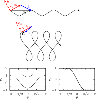
Figure 1: Dynamics of a single spin in the cases $Kp_{0}>1$ (top) and $Kp_{0}<1$ (middle). The momentum $\mathbf{p}_{i}=\mathbf{p}_{0}$ is conserved, the spin $\mathbf{s}_{i}$ oscillates around the direction given by $\mathbf{p}_{i}$ with a frequency $\sqrt{Kp_{0}}$. The velocity $\dot{\mathbf{r}}_{i}$ is then entirely set by Eq. (9a). The plots in the bottom row show that only the $x$-components of the trajectories differ, whereas the $y$-components oscillate on the same trajectory.

Using the conservation of the angular momentum $\mathcal{L}=-y(t)p_{0}+\dot{\theta}$ (see footnote 1), one finds $y(t)=y(0)+({\dot{\theta}}(t)-{\dot{\theta}(0)})/p_{0}$. The motion of the particle, perpendicular to the direction of its momentum, follows the periodic motion of $\dot{\theta}$. The dynamics along the direction of the momentum is more complicated. From Eq. (6a) one has $\dot{x}=p_{0}-K\cos\theta$. For small enough $K$, $K/p_{0}<1$, the particle always moves in the direction of its momentum. However, for larger K, the motion strongly depends on the dynamics of $\theta$; and, for small $\theta$, that is when the spin points to a direction close to that of the momentum, the particle moves into the opposite direction! This counter-intuitive behavior is deeply rooted in the conservation of $\mathbf{p}=\dot{\mathbf{r}}_{i}+K\mathbf{s}$. In the following we shall see that the constraints imposed on the dynamics by the conservation laws, together with the coupling between the spins and the velocities, lead at the mean-field level to the onset of collective motion.

3 Statistical description

3.1 Distribution of microscopic configurations

Starting from the Hamiltonian formulation of the model a Liouville equation can be written for the probability density function of the phase-space point $\mathcal{C}=({\mathbf{r}}^{N},\theta^{N},{\mathbf{p}}^{N},\omega^{N})$. It follows that at equilibrium the probability distribution is a function of the conserved quantities of the dynamics, namely the energy $E$ and the linear momentum $\mathbf{P}$. In the microcanonical ensemble, the conserved quantities cannot be exchanged with the environment; they have constant values $E_{0}$ and ${\mathbf{P}}_{0}$ respectively, and the distribution $\mathcal{P}(\mathcal{C})$ is given by

$$\mathcal{P}_{\text{mc}}(\mathcal{C})=\frac{1}{\Omega}\,\delta(E-E_{0})\delta(\mathbf{P}-\mathbf{P}_{0}),$$ (21)

where $\Omega$ is the microcanonical partition function, defined by normalizing $\mathcal{P}_{\text{mc}}(\mathcal{C})$ to $1$. In other words, all configurations with the same values of the conserved quantities are equally probable.

In practice, it is more convenient from a computational viewpoint to work in the canonical ensemble where the conserved quantities are exchanged with a reservoir. The probability measure in the canonical ensemble is then given by

$$\mathcal{P}(\mathcal{C})=\frac{1}{Z(\beta,\boldsymbol{\alpha})}e^{-\beta(E-\boldsymbol{\alpha}\cdot\mathbf{P})},$$ (22)

where $\beta$ and $\boldsymbol{\alpha}$ are intensive control parameters of the reservoir that determine the thermal averages of $E$ and $\mathbf{P}$ ($\beta$ denotes, as usual, the inverse temperature).

3.2 Computation of average moments

The distribution (22) of the microscopic configurations can be written more explicitly as

$$P(\mathbf{r}^{N},\theta^{N},\mathbf{p}^{N},\omega^{N})=\frac{1}{Z(\beta,\boldsymbol{\alpha})}\prod_{i=1}^{N}\phi(\mathbf{p}_{i},\theta_{i},\omega_{i})\prod_{i<k}\psi(r_{ik},\theta_{ik})$$ (23)

with

$$\phi(\mathbf{p}_{i},\theta_{i},\omega_{i}) =\exp\Bigl{[}-\beta\Bigl{(}\frac{{\mathbf{p}}_{i}^{2}}{2}+\frac{\omega_{i}^{2}}{2}-\mathbf{h}\cdot\mathbf{s}_{i}-(\boldsymbol{\alpha}{+}K{\mathbf{s}}_{i})\cdot{\mathbf{p}}_{i}\Bigr{)}\Bigr{]}$$

$$\psi(r_{ik},\theta_{ik}) =\exp\Bigl{(}\beta j(r_{ik})\cos\theta_{ik}\Bigr{)}\,,$$ (24)

and where

$$Z(\beta,\boldsymbol{\alpha})=Z_{\omega}\int d\theta^{N}Z_{p}(\theta^{N})\,\,Z_{r}(\theta^{N})$$ (25)

is the partition function, with

$$Z_{\omega} =\prod_{i=1}^{N}\int d\omega_{i}\,e^{-\beta\frac{\omega_{i}^{2}}{2}}$$ (26)

$$Z_{p}(\theta^{N}) =\prod_{i=1}^{N}\int d\mathbf{p}_{i}\,e^{-\beta\bigl{(}\frac{{\mathbf{p}}_{i}^{2}}{2}-(\boldsymbol{\alpha}+K{\mathbf{s}}_{i})\cdot{\mathbf{p}}_{i}-\mathbf{h}\cdot\mathbf{s}_{i}\bigr{)}}$$ (27)

$$Z_{r}(\theta^{N}) =\int d\mathbf{r}^{N}\prod_{i<k}e^{\beta j(r_{ik})\cos\theta_{ik}}.$$ (28)

From the distribution (23), one can easily compute the first and second moments of the momenta $\mathbf{p}_{i}$ and $\omega_{i}$. For the first moments, one finds $\langle\omega_{i}\rangle=0$ and

$$\langle{\mathbf{p}}_{i}\rangle=\boldsymbol{\alpha}+K\langle\mathbf{s}_{i}\rangle.$$ (29)

Using Eq. (6a) in Eq. (29) yields $\boldsymbol{\alpha}=\langle\dot{\mathbf{r}}_{i}\rangle$. Taking the sum over all particles and dividing by $N$ then leads to

$$\boldsymbol{\alpha}=\langle\mathbf{V}\rangle.$$ (30)

This relation, which shows that the intensive parameter $\boldsymbol{\alpha}$ associated to the conservation of momentum is the averaged velocity of the center of mass is not specific to the present model. It is a general property of equilibrium systems [34]. However, in the presence of Galilean invariance one can arbitrarily set $\langle\mathbf{V}\rangle=0$ and safely ignore $\boldsymbol{\alpha}$ in the partition function. Here because of the broken Galilean invariance we shall on the contrary keep it as a true and independent intensive thermodynamic parameter. Inserting Eq. (30) into Eq. (29), we end up with

$$\langle{\mathbf{p}}_{i}\rangle=\langle\mathbf{V}\rangle+K\langle\mathbf{s}_{i}\rangle,$$ (31)

which can be seen as a ‘local’ counterpart of Eq. (11).

For the second moment, one finds a generalization of the equipartition relations, with $kT=\beta^{-1}$,

$$\langle\omega_{i}^{2}\rangle =kT,$$ (32)

$$\left(\langle{\mathbf{p}}_{i}^{2}\rangle-\langle{\mathbf{p}}_{i}\rangle^{2}\right)-K^{2}\left(\langle{\mathbf{s}}_{i}^{2}\rangle-\langle{\mathbf{s}}_{i}\rangle^{2}\right) =2kT.$$ (33)

Hence not only are the average values of momentum and spin related, as could have been anticipated from Eq. (11), but so are also their fluctuations. Note however that the temperature is not proportional to the total kinetic energy because of the coupling between the translational velocities and the spins.

3.3 Phase transition in the fully connected model

We now study the behavior of the mean magnetization as a function of temperature and center of mass velocity (or equivalently, $\boldsymbol{\alpha}$). To keep the discussion at a simple enough level, we focus on the fully connected geometry, which is akin to a mean-field approximation (note that the momenta ${\mathbf{p}}_{i}$ and spins ${\mathbf{s}}_{i}$ however remain two-dimensional vectors). In this case, the interaction amplitude $j(|\mathbf{r}_{i}-\mathbf{r}_{k}|)$ is simply a constant, independent of the distance between particles. To ensure that energy remains extensive, we take this constant to be equal to $1/N$. The interaction term can then be rewritten as follows

$$\frac{1}{N}\sum_{i=1}^{N}\sum_{k(\neq i)}{\mathbf{s}_{i}}\cdot{\mathbf{s}_{k}} =\frac{1}{N}\sum_{i=1}^{N}\mathbf{s}_{i}\cdot\Bigl{(}\sum_{k=1}^{N}\mathbf{s}_{k}-\mathbf{s}_{i}\Bigr{)}$$

$$=N\mathbf{m}^{2}-1,$$ (34)

where $\mathbf{m}(\theta^{N})=N^{-1}\sum_{i=1}^{N}\mathbf{s}_{i}$ is the magnetization per spin. Disregarding the constant term (which amounts to a shift in the energy reference), the integrations of Eqs. (26), (27) and (28) over $\omega^{N}$, $\mathbf{r}^{N}$ and $\mathbf{p}^{N}$ are readily computed, yielding

$$Z(\beta,\boldsymbol{\alpha},N,V)=\Bigl{(}\frac{2\pi}{\beta}\Bigr{)}^{\frac{3N}{2}}\,V^{N}\,e^{\frac{\beta}{2}N(K^{2}+\boldsymbol{\alpha}^{2})}\,Z_{\theta}$$ (35)

where $V$ is the volume occupied by the system. The integral that remains to be computed is

$$Z_{\theta}=\int d\theta^{N}\,e^{\frac{1}{2}N\beta\mathbf{m}^{2}+N\beta\mathbf{m}\cdot(K\boldsymbol{\alpha}+\mathbf{h})},$$ (36)

where one recognizes the mean field partition function of the conventional XY-model in the presence of an external field $\mathbf{h}_{\text{eff}}=K\boldsymbol{\alpha}+\mathbf{h}$ [35]. Following standard techniques (see Appendix A), one finds

$$Z_{\theta}=\frac{N\beta}{2\pi}\int du_{1}du_{2}\,e^{-N\beta\mathcal{F}(\mathbf{u})},$$ (37)

where the function $\mathcal{F}(\mathbf{u})$ is given by

$$\mathcal{F}(\mathbf{u})=\frac{\mathbf{u}^{2}}{2}-\frac{1}{\beta}\ln\bigl{[}2\pi I_{0}\bigl{(}\beta\gamma(\mathbf{u})\bigr{)}\bigr{]}$$ (38)

with $I_{n}$, the modified Bessel function of order $n$ and $\gamma(\mathbf{u})=\left|\boldsymbol{\gamma}(\mathbf{u})\right|=\left|K\boldsymbol{\alpha}+\mathbf{h}+\mathbf{u}\right|$. In the large $N$ limit, the integral in Eq. (37) can be computed using the saddle point approximation, yielding to exponential order

$$Z_{\theta}\sim e^{-N\beta\mathcal{F}(\mathbf{u}^{*})}$$ (39)

where the saddle-point $\mathbf{u}^{*}(\boldsymbol{\alpha},\beta,\mathbf{h})$ is given by

$$\frac{\partial\mathcal{F}}{\partial\mathbf{u}}(\mathbf{u}^{*})=\mathbf{u}^{*}-\frac{I_{1}(\beta\gamma(\mathbf{u}^{*}))}{I_{0}(\beta\gamma(\mathbf{u}^{*}))}\,\hat{\boldsymbol{\gamma}}(\mathbf{u}^{*})=0$$ (40)

with $\hat{\boldsymbol{\gamma}}(\mathbf{u}^{*})$ the unit vector $\boldsymbol{\gamma}(\mathbf{u}^{*})/\gamma(\mathbf{u}^{*})$. Using Eq. (35) and Stirling’s approximation, the free energy density $f$ then reads

$$f(\beta,\boldsymbol{\alpha},N/V):=-\frac{kT}{N}\ln\frac{Z(\beta,\boldsymbol{\alpha},N,V)}{N!}\\ \sim\mathcal{F}(\mathbf{u}^{*})-\frac{1}{\beta}\Bigl{(}\frac{3}{2}\ln\frac{2\pi}{\beta}-\ln\frac{N}{V}+1\Bigr{)}-\frac{\boldsymbol{\alpha}^{2}}{2}.$$ (41)

It is a function of intensive variables only. Finally the average magnetization $\langle\mathbf{m}\rangle$ per particle is:

$$\langle\mathbf{m}\rangle=-\frac{\partial f}{\partial\mathbf{h}}=-\frac{\partial\mathbf{u}^{*}}{\partial\mathbf{h}}\frac{\partial\mathcal{F}}{\partial\mathbf{u}}(\mathbf{u}^{*})-\frac{\partial\mathcal{F}}{\partial\mathbf{h}}(\mathbf{u}^{*}).$$ (42)

Since $\partial\mathcal{F}/\partial\mathbf{u}(\mathbf{u}^{*})=0$, we end up with $\langle\mathbf{m}\rangle=-\frac{\partial\mathcal{F}}{\partial\mathbf{h}}(\mathbf{u}^{*})$. Combining this last result with the definition of $\boldsymbol{\gamma}$ and Eqs. (38) and (40), we get that $\langle\mathbf{m}\rangle=\mathbf{u}^{*}$. Hence $\langle\mathbf{m}\rangle$ can be obtained from the self-consistent equation (40), simply replacing $\mathbf{u}^{*}$ by $\langle\mathbf{m}\rangle$.

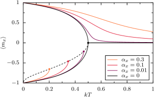
Figure 2: Magnetization of the fully connected model, in the absence of external field $(\mathbf{h}=\mathbf{0})$, but with non-zero effective field $\mathbf{h}_{\text{eff}}=K\boldsymbol{\alpha}$. Solid curves are obtained from numerically minimizing $\mathcal{F}(\mathbf{u})$. Parameters are $K=1$, $\alpha_{y}=0$.

Using $\frac{\partial\ln Z}{\partial\beta}=-\langle H\rangle+\boldsymbol{\alpha}\cdot\langle\mathbf{P}\rangle$, we also obtain the average energy per particle $\langle e\rangle=\langle H\rangle/N$:

$$\langle e\rangle=\frac{3}{2\beta}+\frac{\boldsymbol{\alpha}^{2}-{\mathbf{u}^{*}}^{2}}{2}-\mathbf{h}\cdot\mathbf{u}^{*}.$$ (43)

Eq. (40) can be solved numerically, the result being depicted in Fig. 2 for the case $K=1$ in the absence of external field $(\mathbf{h}=\mathbf{0})$. Without loss of generality we choose $\boldsymbol{\alpha}$ in the $x$-direction. When $\boldsymbol{\alpha}=\mathbf{0}$, there is a phase transition from an isotropic to a magnetized phase at $kT_{c}=1/2$. For nonzero values of $\boldsymbol{\alpha}$, we find in the upper half of the figure smooth magnetization curves which demonstrate that the coupling between the spins and the particle velocities is encompassed into an effective field $\mathbf{h}_{\text{eff}}=\mathbf{h}+K\boldsymbol{\alpha}$: as long as $K>0$, the average velocity of the center of mass acts as an external field, polarizing the spins. This nontrivial effect of the center-of-mass velocity is directly related to the loss of Galilean invariance. Actually, starting from the more general coupling term given in Eq. (19), one finds that the effective external field $\mathbf{h}_{\text{eff}}$ is changed into

$$\mathbf{h}_{\text{eff}}=\mathbf{h}+K(1-\eta)\boldsymbol{\alpha},$$ (44)

so that the contribution from $\boldsymbol{\alpha}$ to the effective field vanishes for $\eta=1$, when Galilean invariance is recovered.

In its lower half, Figure 2 shows further solutions. These are also obtained from minimizing $\mathcal{F}(\mathbf{u})$, but here the minima are local ones. In these solutions, the magnetization $\mathbf{M}$ is opposite to the center-of-mass velocity $\boldsymbol{\alpha}$. We can already anticipate that these local minima are essential to the low temperature physics of the model in the microcanonical ensemble: for a system with vanishing fixed total momentum, Eq. (11) imposes $\langle\mathbf{m}\rangle=-K\boldsymbol{\alpha}$ and the system will select the minima for which $\boldsymbol{\alpha}$ and $\langle\mathbf{m}\rangle$ are anti-aligned.

Although observing an ordering transition in a mean-field framework usually does not come as a surprise, let us emphasize that the present transition is non-standard even at mean-field level, in the sense that collective motion cannot be observed in equilibrium systems where momentum is either conserved or exchanged with a substrate, as long as the relation $\mathbf{P}=N\mathbf{V}$ is valid. The transition clearly relies on the coupling between spin and velocity, and disappears for $K=0$.

Also, the above results only hold for the fully-connected model, that is at the mean-field level. In the case of the standard two-dimensional XY-model, it is very well known that mean-field approximations erroneously predict a transition towards a true long-range ordered phase at low temperature, which in two dimensions is replaced by the celebrated Berezinskii–Kosterlitz–Thouless transition towards a quasi-long-range ordered phase, with zero magnetization, but infinite correlation length of its fluctuations [26, 27, 28]. Physically, long-range order in the two-dimensional XY-model is destroyed by the low-energy spin-wave excitations associated with the invariance of the dynamics under a continuous rotation of the spins. In the present case, we have seen in section 2.2 that this symmetry is absent for $K\neq 0$ when globally rotating the spins alone. One can however argue that a more general transformation, rotating both the spins and the velocities, should be applied to restore the Mermin-Wagner theorem. When a reservoir imposes $\boldsymbol{\alpha}$, or when the conserved momentum has a fixed value $\mathbf{P}_{0}\neq 0$, isotropy is actually broken. Yet, when $\mathbf{P}_{0}=0$, the system is isotropic and long wave-length excitations involving spins and velocities may be expected to destroy long-range order.

4 Molecular Dynamics simulations

In order to perform numerical simulations of the dynamics described by the equations of motion (9), one needs to specify the spatial dependence of the ferromagnetic interaction. Doing so, one notices that the interaction not only leads to alignment of the spins but also to attraction/repulsion of interacting spins, depending on their relative orientations. Typically, spins of similar direction cluster together while oppositely pointed spins repel each other. An aligned phase is thus expected to end up with all particles being very close together. In order to avoid this undesired behavior, we add a repulsive potential $U(r_{ik})$ as introduced in Eq. (1a), which translates into a repulsive force term in Eq. (9b). In the following, we set

$$j(r)=(1-r)^{2}\quad\text{and}\quad U(r)=4(1-r)^{4}$$ (45)

for $r\leq 1$ and $j(r)=U(r)=0$ for $r\geq 1$. The interaction range is thus one unit length and the two interactions are of the same magnitude for $r=1/2$.

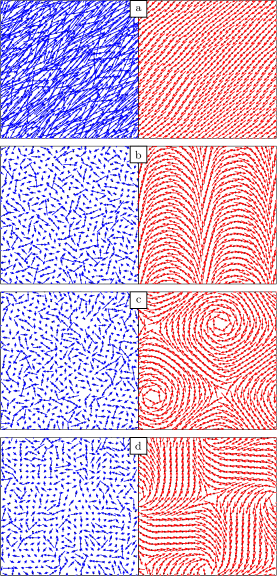
Figure 3: (a) Ground state for $K=0.1$. (b–d) Candidates for ground states for $K=0.3,0.5,1.0$. Black dots indicate particle positions in the $x,y$-plane; left: blue arrows are $\dot{\mathbf{r}}_{i}$; right: red arrows are $\mathbf{s}_{i}$. $N=500,\rho=3.55,\zeta=0.9999$.

We perform simulations in the microcanonical ensemble in square boxes of size $L\times L$, with periodic boundary conditions and a fixed density of particles $\rho=N/L^{2}=3.55$; $N=[256,500,1000]$. The equations of motion are integrated using a standard fourth-order Runge–Kutta approximation. The total energy $E_{0}$ and momentum $\mathbf{P}_{0}$ are set by the initial condition. In the following, we shall always start from initial conditions where all positions and spins orientations are random, and all velocities, both $\dot{\mathbf{r}}_{i}$ and $\omega_{i}$, are zero. Hence in the initial conditions the total magnetization $\mathbf{M}_{0}=\mathbf{0}$ and the velocity of the center of mass $\mathbf{V}_{0}=\mathbf{0}$, so that the total momentum $\mathbf{P}_{0}=\mathbf{0}$. Typically, starting from such an initial condition, the system reaches a disordered steady state. However, from the phase transition diagram in Fig. 2, one would expect that a system prepared with low enough energy will also be at low temperature and will thus evolve towards an ordered state with nonzero magnetization $\langle\mathbf{m}\rangle$. If this were the case, because $\mathbf{P}=\mathbf{0}$ is conserved, the system would acquire a finite velocity of its center-of-mass $\mathbf{V}=-K\langle\mathbf{m}\rangle$: collective motion would set in spontaneously.

We first look for the ground state for different values of $K$. We perform slow annealing of the system by removing rotational kinetic energy at a constant rate: every $100$ integration steps, a factor $\zeta<1$ is applied to all $\omega_{i}$. We checked that the annealing rate was small enough to ensure that we observed (statistically) the same result for different rates. We also checked that the total momentum $\mathbf{P}$ remained null during the annealing procedure. Figure 3 displays the final states obtained from this annealing procedure in a system of $N=500$ particles. One observes quite a rich phase behavior: for $K=0.1$ all spins are indeed aligned as in panel (a) and, as anticipated, all velocities align in the opposite direction, so that collective motion is present. For $K=0.3$, $0.5$, $0.7$, and $1$ we observe three kinds of different final states occurring at random, which are depicted in panels (b) to (d). They have large-scale structure in their magnetization field, such that the total magnetization vanishes; as a result $\mathbf{V}=\mathbf{0}$: the velocities fluctuate independently, and no global motion takes place. The three states in Fig.3b–d can be seen as candidates for the ground state, representing local minima in a free-energy landscape. The frequency at which one of these states is picked by the annealing process depends on $K$ and on the number of particles $N$. For $N=500$, we could only find the magnetized ground state for $K=0.1$.

We now investigate how magnetization resists thermal fluctuations. Figure 4 displays the phase diagram for systems with zero total momentum $\mathbf{P}=\mathbf{0}$. To obtain it, we slowly anneal the system from a disordered initial state with energy $E_{0}$, but stop the annealing at a beforehand chosen value of $E$, which is then conserved. We then wait for the system to relax and start to average the magnetization. One can see that for sufficiently small $K$ magnetization survives on a finite range of energy.

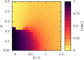
Figure 4: Parameter-dependence of the average magnetization in the steady state as a function of the prescribed energy $E$. Values of $K$ run from $0.01$ to $0.5$ in equal steps. In all simulations $\mathbf{P}=\mathbf{0}$, $N=256$, $\zeta=0.999$, $\rho=3.55$.

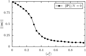
Figure 5: Average magnetization in microcanonical simulations, as a function of the measured temperature. Colors/linestyles correspond to different momenta, symbols indicate system sizes: $N=256$ (square), $500$ (circle), $1000$ (triangle). In all simulations $K=0.1$, $\zeta=0.99$, $\rho=3.55$.

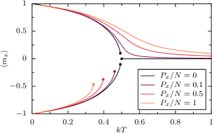
Figure 6: Curves of constant $\mathbf{P}$ in the fully connected model. $K=0.1$, $\mathbf{h}=\mathbf{0}$, $\alpha_{y}=0$, $P_{y}=0$.

Focusing on the case $K=0.1$, for which collective motion is indeed observed (at least in the finite size system), we investigate the transition towards the disordered state at high energy. The simulation data is plotted in Fig. 5 for different system sizes and different momenta. Here, for the purpose of comparison with the canonical case, we choose to plot the magnetization as a function of $kT$, where the temperature is measured using the rotational velocity fluctuations, as prescribed by Eq. (32). A crossover from low to high values of the magnetization is clearly visible when temperature is decreased. To better compare it with the canonical calculation of Sec. 3.3 above, although no quantitative agreement is to be expected due to the finite range of spin interactions $j(r)$ and the addition of the repulsive potential $U(r)$, we invert the canonical relations $\langle e\rangle(\beta,\boldsymbol{\alpha})$ and $\langle\mathbf{P}\rangle(\beta,\boldsymbol{\alpha})$ from Eqs. (29) and (43). We thus obtain in Fig. 6 the magnetization computed in the canonical ensemble as a function of ($E$, $\mathbf{P})$ or more conveniently ($\beta$,$\mathbf{P}$). For finite $\mathbf{P}$ continuous branches of solution relate the disordered state at high temperature to the homogeneous magnetized state at low temperature. These branches resemble very much those obtained from the microcanonical simulations (Fig. 5). The zero-momentum case is very peculiar: there is a finite range of energy, or $kT$, where no solutions with homogeneous magnetization exist. Because of finite-size effects, this peculiarity could not be captured in the microcanonical simulations. Also, from the data in Fig. 5 it is not yet clear whether the magnetization at $kT>0$ survives the limit of large systems, $N\to\infty$. The transition shifts more and more to the left, but more systematic investigation would be necessary to know whether it converges to a nonzero critical temperature. As a first step we looked at finite size effects, focusing on the ground state. We ran the annealing protocol on ten systems of size $N=2000$, for respectively $K=0.1$ and $0.3$. By increasing the system size, the fully ordered state is now replaced by an inhomogeneous state with zero total magnetization, in a way similar to the effect of increasing $K$ at a given system size (Fig. 3b–d). The crossover size is larger for smaller $K$. Given that for $K=0$ no long-range order is expected, these observations suggest that long-range order may not survive in the thermodynamic limit for all $K$. Obtaining the precise scaling in $K$, temperature and system size would require a deeper analysis, both theoretically and numerically, which is beyond the scope of the present work.

5 Discussion and conclusion

In order to discuss the above observations, let us recall that the Hamiltonian can be interpreted as the sum of the kinetic and potential energies, in which the peculiarity of the present model is entirely encoded in the unusual relation $\dot{\mathbf{r}}_{i}=\mathbf{p}_{i}-K\mathbf{s}_{i}$ (see Eq. (10) in section 2.1). To obtain low energy states, the system should (i) minimize its kinetic energy, thus decrease all $|\dot{\mathbf{r}}_{i}|$ and generate small $|\mathbf{V}|$ states; (ii) align its spins, thus favoring states with large $|\mathbf{M}|$. However this is incompatible with the constraint $\mathbf{P}=N\mathbf{V}+K\mathbf{M}=\mathbf{0}$. In particular, because the constraint imposes $N|\mathbf{V}|=K|\mathbf{M}|$, the spin alignment potentially leads to large kinetic energy. This dynamical frustration is all the more important that $K$ is large. This is why decreasing $K$ is a way to favor ordered states at low energy. At larger $K$, the system selects zero magnetization states, at the price of generating bend and splay in the spin field. Also the larger the system, the smaller are these distortions. This is why only small $K$ and small size system exhibit homogeneously ordered phases.

In summary, we have proposed in this paper a conservative model of particles in which velocities and spins are coupled. Starting from a Lagrangian formulation and deriving from it the Hamiltonian one, we obtained using the symmetries of the problem that the total (generalized) linear momentum is conserved but is no longer proportional to the center-of-mass velocity. We then studied the effect of this important change on spin statistics and on collective motion. Our main findings are that (i) collective motion sets in starting from an immobile system, provided that the spins are able to align ferro-magnetically as observed in particular in the fully connected geometry, or in small enough systems, and (ii) the parameter $\boldsymbol{\alpha}=\left<\mathbf{V}\right>$ thermodynamically conjugated to linear momentum acts as an external magnetic field on the magnetization.

More generally, the main interest of the present model is to show that collective motion, albeit perhaps of a nonstandard type, is possible even for conservative models, provided that spins and velocities are coupled. Although it is hard to imagine a physical realization of the present model, the latter however has the virtue of showing that, at least at a conceptual level, energy dissipation is not a necessary ingredient for collective motion. Also, in a spirit similar to that of [24] it brings the transition to collective motion on a theoretical playground where a number of tools have been developed to characterize phase transitions.

The present paper aimed at introducing the model, discuss its symmetries and the crucial role of the broken Galilean invariance. As such, it remains very preliminary. We have only looked at the mean field scenario, and illustrated the model behavior on a few MD simulations. A number of perspectives can be mentioned. Obviously one would like to investigate more systematically the phase diagram of the system and the existence of a phase transition in the infinite size limit. Also, it would be interesting to make progress in the direction of the theoretical analysis of the model in finite dimension. In particular two limits of interest are $K\rightarrow 0$, which corresponds to the intricate physics of the XY-model and its Berezinskii-Kosterlitz-Thouless transition, and $\eta\rightarrow 1$, where Galilean invariance is recovered. Perturbative approaches using $K$ and/or $\eta$ as small parameters could be a way to tackle this theoretical analysis. Besides, we have not yet explored the possibility that the model might be invariant under a more complicated transformation than the Galilean one, in analogy to the Lorentz transform that arises in the context of electromagnetism. Whether such a transformation exists is however far from clear; in electromagnetic systems, the invariance under the Lorentz transform is only obtained when considering relativistic mechanics, while our model remains within the realm of Newtonian mechanics.

Appendix A Computation of the mean-field partition function

In this appendix, we provide the detailed derivation of the mean-field free energy $\mathcal{F(\mathbf{u})}$ given in Eq. (38). Starting from Eq. (36), we need to compute the following integral,

$$Z_{\theta}=\int d\theta^{N}\,e^{\frac{1}{2}N\beta\mathbf{m}^{2}+N\beta\mathbf{m}\cdot(K\boldsymbol{\alpha}+\mathbf{h})}$$ (46)

To write the exponential function as a linear function of $\mathbf{m}$ we use the Hubbard–Stratonovich transformation,

$$e^{b^{2}/2a}=\sqrt{\frac{a}{2\pi}}\int^{\infty}_{-\infty}du\,e^{-\frac{1}{2}au^{2}+bu}.$$ (47)

Considering for instance the $x$-component, and setting $b=N\beta m_{x}$ and $a=N\beta$, one gets

$$e^{\frac{1}{2}N\beta m_{x}^{2}}=\sqrt{\frac{N\beta}{2\pi}}\int^{\infty}_{-\infty}du_{1}\,e^{-\frac{1}{2}N\beta u_{1}^{2}+N\beta m_{x}u_{1}}.$$ (48)

Combining the two directions $x$ and $y$ yields for the partition function, using the notation $\mathbf{u}=(u_{1},u_{2})$,

$$Z_{\theta}=\frac{N\beta}{2\pi}\int du_{1}du_{2}d\theta^{N}\,e^{-N\beta(\frac{\mathbf{u}^{2}}{2}-\boldsymbol{\gamma}(\mathbf{u})\cdot\mathbf{m})},$$ (49)

where

$$\boldsymbol{\gamma}(\mathbf{u})\equiv K\boldsymbol{\alpha}+\mathbf{h}+\mathbf{u}.$$ (50)

Up to a shift on the variable $\theta_{i}$ (that is irrelevant since integration is on the circle), the scalar product $\boldsymbol{\gamma}(\mathbf{u})\cdot\mathbf{m}$ can be expressed as

$$\boldsymbol{\gamma}(\mathbf{u})\cdot\mathbf{m}=\frac{1}{N}\sum_{i}\boldsymbol{\gamma}(\mathbf{u})\cdot\mathbf{s}_{i}=\frac{1}{N}\sum_{i}\gamma(\mathbf{u})\cos\theta_{i}$$ (51)

where $\gamma(\mathbf{u})=|\boldsymbol{\gamma}(\mathbf{u})|$. We end up with

$$Z_{\theta}=\frac{N\beta}{2\pi}\int du_{1}du_{2}\,e^{-N\beta\mathbf{u}^{2}/2}\prod_{i=1}^{N}\int_{-\pi}^{\pi}d\theta_{i}\,e^{\beta\gamma(\mathbf{u})\cos\theta_{i}}$$ (52)

Denoting $I_{0}(x)$ the modified Bessel function of order $0$:

$$I_{0}(x)=\frac{1}{2\pi}\int_{-\pi}^{\pi}d\theta\,e^{x\cos\theta}$$ (53)

we finally get Eqs. (37) and (38) of the main text.

References

- [1] Ramaswamy S 2010 Annu Rev Conden Ma P 1 323–345
- [2] Marchetti M C, Joanny J F, Ramaswamy S, Liverpool T B, Prost J, Rao M and Simha R A 2013 Rev. Mod. Phys. 85 1143–1189
- [3] Schaller V and Bausch A R 2013 Proceedings of the National Academy of Sciences 110 4488–4493
- [4] Schaller V, Weber C, Frey E and Bausch A R 2011 Soft Matter 7 3213
- [5] Schaller V, Weber C, Semmrich C, Frey E and Bausch A R 2010 Nature 467 73–77
- [6] Sumino Y, Nagai K H, Shitaka Y, Tanaka D, Yoshikawa K, Chaté H and Oiwa K 2012 Nature 483 448–452
- [7] Chen X, Dong X, Be’er A, Swinney H L and Zhang H P 2012 Phys. Rev. Lett. 108 148101
- [8] Zhang H P, Be’er A, Florin E L and Swinney H L 2010 Proceedings of the National Academy of Sciences of the United States of America 107 13626–13630
- [9] Buhl J, Sumpter D J T, Couzin I D, Hale J J, Despland E, Miller E R and Simpson S J 2006 Science 312 1402
- [10] Ballerini M, Cabibbo N, Candelier R, Cavagna A, Cisbani E, Giardina I, Lecomte V, Orlandi A, Parisi G, Procaccini A and others 2008 Proceedings of the National Academy of Sciences 105 1232
- [11] Cavagna A, Del Castello L, Giardina I, Grigera T, Jelic A, Melillo S, Mora T, Parisi L, Silvestri E, Viale M and Walczak A M 2015 J Stat Phys 158 601–627
- [12] Palacci J, Cottin-Bizonne C, Ybert C and Bocquet L 2010 Phys. Rev. Lett. 105 –
- [13] Theurkauff I, Cottin-Bizonne C, Palacci J, Ybert C and Bocquet L 2012 Phys. Rev. Lett. 108 268303
- [14] Bricard A, Caussin J B, Desreumaux N, Dauchot O and Bartolo D 2013 Nature 503 95–98
- [15] Palacci J, Sacanna S, Steinberg A P, Pine D J and Chaikin P 2013 Science 339 936–940
- [16] Thutupalli S, Seemann R and Herminghaus S 2011 New Journal of Physics 13 073021
- [17] Izri Z, van der Linden M N, Michelin S and Dauchot O 2014 PRL 113 248302
- [18] Narayan V, Ramaswamy S and Menon N 2007 Science 317 105–108
- [19] Deseigne J, Dauchot O and Chaté H 2010 Phys. Rev. Lett. 105
- [20] Deseigne J, Léonard S, Dauchot O and Chaté H 2012 Soft Matter 8 5629
- [21] Kumar N, Soni H, Ramaswamy S and Sood A K 2014 Nature Communications 5
- [22] Vicsek T, Czirók A, Ben-Jacob E, Cohen I and Shochet O 1995 Phys. Rev. Lett. 75 1226–1229
- [23] Toner J and Tu Y 1995 Phys. Rev. Lett. 75 4326–4329
- [24] Solon A P and Tailleur J 2013 PRL 111
- [25] Mermin N D and Wagner H 1966 Phys. Rev. Lett. 17 1133–1136
- [26] Berezinskii V 1970 Zh. Eksp. Teor. Fiz. 59 907 URL http://www.jetp.ac.ru/cgi-bin/e/index/e/32/3/p493?a=list
- [27] Kosterlitz J M and Thouless D J 1973 Journal of Physics C: Solid State Physics 6 1181
- [28] Kosterlitz J M 1974 Journal of Physics C: Solid State Physics 7 1046
- [29] Chaté H, Ginelli F, Grégoire G and Raynaud F 2008 Phys. Rev. E 77 –
- [30] Grégoire G and Chaté H 2004 Phys. Rev. Lett. 92 025702
- [31] Toner J 2012 Phys. Rev. E 86 031918–9
- [32] Weber C A, Hanke T, Deseigne J, Léonard S, Dauchot O, Frey E and Chaté H 2013 Phys. Rev. Lett. 110 208001
- [33] Lam K D N T, Schindler M and Dauchot O 2015 New J. Phys. 17 113056
- [34] Diu B, Guthmann C, Lederer D and Roulet B 1989 Physique statistique (Editions Hermann, Paris) ISBN 978-2705666866
- [35] Chaikin P M and Lubensky T C 2000 Principles of condensed matter physics (Cambridge Univ Press)