Dirty bosons in a three-dimensional harmonic trap

Abstract

We study a three-dimensional Bose-Einstein condensate in an isotropic harmonic trapping potential with an additional delta-correlated disorder potential at both zero and finite temperature and investigate the emergence of a Bose-glass phase for increasing disorder strength. To this end, we revisit a quite recent non-perturbative approach towards the dirty boson problem, which relies on the Hartree-Fock mean-field theory and is worked out on the basis of the replica method, and extend it from the homogeneous case to a harmonic confinement. At first, we solve the zero-temperature self-consistency equations for the respective density contributions, which are obtained via the Hartree-Fock theory within the Thomas-Fermi approximation. Additionally we use a variational ansatz, whose results turn out to coincide qualitatively with those obtained from the Thomas-Fermi approximation. In particular, a first-order quantum phase transition from the superfluid phase to the Bose-glass phase is detected at a critical disorder strength, which agrees with findings in the literature. Afterwards, we consider the three-dimensional dirty boson problem at finite temperature. This allows us to study the impact of both temperature and disorder fluctuations on the respective components of the density as well as their Thomas-Fermi radii. In particular, we find that a superfluid region, a Bose-glass region, and a thermal region coexist for smaller disorder strengths. Furthermore, depending on the respective system parameters, three phase transitions are detected, namely, one from the superfluid to the Bose-glass phase, another one from the Bose-glass to the thermal phase, and finally one from the superfluid to the thermal phase.

I Introduction

The combined effect of disorder and two-particle interactions in the dirty boson problem yields a competition between localization and superfluidity Intro-11 . Experimentally, the dirty boson problem was first studied with superfluid helium in porous media like aerosol glasses (Vycor), where the pores are modeled by statistically distributed local scatterers Intro-91 ; Intro-92 ; Intro-93 ; Intro-94 . Disorder in Bose gases appears either naturally as, e.g., in magnetic wire traps Intro-75 ; Intro-76 ; Intro-77 ; Fortagh ; Schmiedmayer , where imperfections of the wire itself can induce local disorder, or it may be created artificially and controllably as, e.g., by using laser speckle fields Intro-78 ; Intro-79 ; Intro-21 ; Goodmann ; Intro-16 . A set-up more in the spirit of condensed matter physics relies on a Bose gas with impurity atoms of another species trapped in a deep optical lattice, so the latter represent randomly distributed scatterers Intro-13 ; Intro-14 . Furthermore, an incommensurate optical lattice can provide a pseudo-random potential for an ultracold Bose gas Lewenstein ; Ertmer ; intro-17 .

The homogeneous dirty boson model is important as it provides a good description at the center of a harmonic trap and, thus, serves as a starting point for treating a harmonic confinement within the Thomas-Fermi approximation. Furthermore, recently it has even become possible to experimentally realize box-like traps Hadzibabic , which approximate the homogeneous case in the thermodynamic limit. The first important theoretical result for the homogeneous dirty boson was obtained by Huang and Meng, who found, within the Bogoliubov theory Intro-7 , that a weak disorder potential with delta correlation leads to a depletion of both the condensate and the superfluid density due to the localization of bosons in the respective minima of the random potential HM-1 . Later on their theory was extended in different research directions. Results for the shift of the velocity of sound as well as for its damping due to collisions with the external field are worked out in Ref. HM-3 . Furthermore, the delta-correlated random potential was generalized to experimentally more realistic disorder correlations with a finite correlation length, e.g., a Gaussian correlation was discussed in Ref. HM-4 and laser speckles are treated at zero HM-6 and finite temperature HM-7 . Also the disorder-induced shift of the critical temperature was analyzed in Refs. HM-5 ; HM-2 . Furthermore, it was shown that dirty dipolar Bose gases yield characteristic directional dependences for thermodynamic quantities due to the emerging anisotropy of superfluidity at zero HM-8 ; HM-9 and finite temperature HM-10 ; Boujam3a1 ; Boujam3a2 . The location of superfluid, Bose-glass, and normal phase in the phase diagram spanned by disorder strength and temperature was qualitatively analyzed for the first time in Ref. Intro-90 on the basis of a Hartree-Fock mean-field theory with the replica method. In addition, increasing the disorder strength at small temperatures yields a first-order quantum phase transition from a superfluid to a Bose-glass phase, where in the latter case all particles reside in the respective minima of the random potential. This prediction is achieved at zero temperature by solving the underlying Gross-Pitaevskii equation with a random phase approximation Navez , as well as at finite temperature by a stochastic self-consistent mean-field approach using two chemical potentials, one for the condensate and one for the excited particles Yukalov1 . Numerically, Monte-Carlo (MC) simulations have been applied to study the homogeneous dirty boson problem. For instance, diffusion MC in Ref. Astrakharchik obtained the surprising result that at zero temperature a strong enough disorder yields a superfluid density, which is larger than the condensate density. Furthermore, worm-algorithm MC was able to determine the dynamic critical exponent of the quantum phase transition from the Bose-glass to the superfluid in two dimensions at zero Monte-Carlo1 and finite temperature Monte-Carlo2 .

Adding a harmonic trap to the dirty Bose gas problem makes it realistic but more complicated to treat than the homogeneous one. Since the collective excitation frequencies of harmonically trapped bosons can be measured very accurately, their change due to disorder was investigated in Ref. Collective-excitations at zero temperature. As the collective excitation frequencies turn out to decrease rapidly with the correlation length of disorder, one would have to reduce the correlation length of the laser speckles in Ref. Intro-79 from $10{\rm\,{\mu m}}$ by a factor of $10$ in order to be able to detect any shift due to the disorder. The expansion of a Bose-Einstein condensate (BEC) at zero temperature in the presence of a random potential was studied in Ref. Boris-trap . Depending on the strength of disorder and the two-particle interaction, a crossover from localization to diffusion was observed. The shape and size of the local minicondensates in the disorder landscape were investigated energetically at zero temperature in Refs. Nattermann ; Natterman2 , where it was deduced that, for decreasing disorder strength, the Bose-glass phase becomes unstable and goes over into the superfluid. At finite temperature the disorder-induced shift of the critical temperature was analyzed for a harmonic confinement in Ref. Timmer . The impact of the random potential upon the quantum fluctuations at finite temperature was also studied in Refs. Gaul-Muller-1 ; Gaul-Muller-2 . Furthermore, based on Ref. Intro-90 , Ref. Paper2 worked out in detail a non-perturbative approach to the dirty boson problem, which relies on the Hartree-Fock theory and the Parisi replica method, for a weakly interacting Bose-gas within a harmonic confinement and a delta-correlated disorder potential at finite temperature. Its application to a quasi one-dimensional BEC at zero temperature Paper1 reveals a redistribution of the minicondensates from the edge of the atomic cloud to the trap center for increasing disorder strengths. Despite all these many theoretical predictions, so far no experiment has tested them quantitatively.

In the present paper we treat analytically the problem of a three-dimensional trapped BEC in a disorder potential on the basis of Ref. Paper2 . To this end, we start by describing the underlying dirty boson model and developing a Hartree-Fock mean-field theory in Section II. Then we treat, as a first step, the zero-temperature case in Section III, which allows us to study the impact of the disorder on the distribution of the condensate density and the Bose-glass order parameter, which quantifies the density of the bosons in the local minima of the disorder potential. We deal first with the simpler homogeneous case, and then we analyze the isotropic harmonically trapped one. Using the corresponding self-consistency equations obtained via the Hartree-Fock mean-field theory, we investigate within the Thomas-Fermi approximation the existence of the Bose-glass phase. We additionally use a variational ansatz, whose results turn out to coincide qualitatively with the ones obtained via the Thomas-Fermi approximation. In Section IV we consider the three-dimensional dirty BEC system to be at finite temperature. We restrict ourselves first to the homogeneous dirty case, after that to the trapped clean case. Afterwards we treat the trapped disordered case at finite temperature using the Thomas-Fermi approximation. This allows us to study the impact of both temperature and disorder fluctuations on the respective components of the density as well as their Thomas-Fermi radii. In particular, three regions coexist, namely, a superfluid region, a Bose-glass region, and a thermal region. Furthermore, depending on the respective system parameters, three phase transitions are detected, one from the superfluid to the Bose-glass phase, another one from the Bose-glass to the thermal phase, where all bosons are in the excited states, and a third one from the superfluid to the thermal phase.

II Hartree-Fock Mean-Field Theory in 3D

The model of a three-dimensional weakly interacting homogeneous Bose gas in a delta-correlated disorder potential was studied within the Hartree-Fock mean-field theory in Ref. Intro-90 by applying the Parisi replica method Intro-36 ; Intro-37 ; Intro-33 . This Hartree-Fock theory is extended in Ref. Paper2 to a harmonic confinement. Let us briefly summarize the main result of Ref. Paper2 , which relies on deriving a semiclassical approximation for the underlying free energy.

We consider a three-dimensional Bose gas in an isotropic harmonic potential $V(\mathbf{r})=M\Omega^{2}\mathbf{r}^{2}/2$ with the trap frequency $\Omega$, the particle mass $M$ and the contact interaction potential $V^{({\rm int})}(\mathbf{r}-\mathbf{r}^{\prime})=g\delta(\mathbf{r}-\mathbf{r}^{\prime})$. The interaction coupling strength $g=4\pi\hslash^{2}a/M$ depends on the s-wave scattering length $a$, which has to be positive in order to obtain a stable BEC. We assume for the disorder potential $U(\mathbf{r})$ that it is homogeneous after performing the disorder ensemble average, denoted by $\overline{\bullet}$, over all possible realizations. Thus, the expectation value of the disorder potential can be set to vanish without loss of generality,

$$\overline{U(\mathbf{r})}=0,$$ (1)

and its correlation function is assumed to be proportional to a delta-function,

$$\overline{U(\mathbf{r}_{1})U(\mathbf{r}_{2})}=D\,\delta(\mathbf{r}_{1}-\mathbf{r}_{2})\,,$$ (2)

where $D$ denotes the disorder strength.

By working out the Hartree-Fock mean-field theory within the replica method, Ref. Paper2 obtains self-consistency equations, which determine the particle density $n(\mathbf{r})$ as well as the order parameter of the superfluid $n_{0}(\mathbf{r})$, representing the condensate density, the order parameter of the Bose-glass phase $q(\mathbf{r})$ defined in Ref. Intro-90 , that stands for the density of the particles being condensed in the respective minima of the disorder potential, and $n_{{\rm th}}\left(\mathbf{r}\right)$, which represents the density of the particles in the excited states. The Hartree-Fock mean-field theory with the help of the replica method and a semiclassical approximation leads to the free energy Paper2 :

$$\mathcal{F} =4\pi\!\int_{0}^{\infty}drr^{2}\Biggl{\{}-g\left[q(r)+n_{0}(r)+n_{{\rm th}}\left(r\right)\right]^{2}-\frac{g}{2}n_{0}^{2}(r)$$

$$\!\!\!\!\!\!+\frac{D}{\hbar}Q_{0}(r)\left[q(r)+n_{0}(r)+n_{{\rm th}}\left(r\right)\right]-\sqrt{n_{0}(r)}$$

$$\!\!\!\!\!\!\times\Biggl{\{}\mu+\frac{\hbar^{2}}{2M}\frac{1}{r^{2}}\frac{\partial}{\partial r}\left(r^{2}\frac{\partial}{\partial r}\right)-2g\left[q(r)+n_{0}(r)+n_{{\rm th}}\left(r\right)\right]$$

$$\!\!\!\!\!\!-V(r)+\frac{D}{\hbar}Q_{0}(r)\Biggr{\}}\sqrt{n_{0}(r)}-2D\sqrt{\pi}\left(\frac{M}{2\pi\hbar^{2}}\right)^{3/2}$$ (3)

$$\!\!\!\!\!\!\times\left[q(r)+n_{0}(r)+n_{{\rm th}}\left(r\right)\right]-\frac{1}{\beta}\left(\frac{M}{2\pi\hbar^{2}\beta}\right)^{3/2}\zeta_{5/2}\left(e^{\beta\mu_{r}(r)}\right)$$

$$\!\!\!\!\!\!\left.\times\sqrt{-\mu+2g\left[q(r)+n_{0}(r)+n_{{\rm th}}\left(r\right)\right]+V(r)-\frac{D}{\hbar}Q_{0}(r)}\right\}.$$

Here all functions only depend on the radial coordinate $r=\left|\mathbf{r}\right|$ due to the assumed spatial isotropy. Furthermore, $\mu$ denotes the chemical potential, $\mu_{r}(r)=\mu-V(r)-2g\left[q(r)+n_{0}(r)+n_{{\rm th}}\left(r\right)\right]-\pi D^{2}\left(\frac{M}{2\pi\hbar^{2}}\right)^{3}$ represents the renormalized chemical potential, and $Q_{0}(r)$ stands for an auxiliary function, which appears within the Hartree-Fock theory:

$$Q_{0}(r) =-2\sqrt{\pi}\hbar{\displaystyle\left(\frac{M}{2\pi\hbar^{2}}\right)^{3/2}}$$

$$\times\left[\sqrt{\pi}D{\displaystyle\left(\frac{M}{2\pi\hbar^{2}}\right)^{3/2}}+\sqrt{-\mu_{r}(r)}\right].$$ (4)

From the thermodynamic relation $N=-\frac{\partial\mathcal{F}}{\partial\mu}$ we obtain

$$N=4\pi\int_{0}^{\infty}r^{2}n(r)dr,$$ (5)

which defines the particle density $n(r)$.

Extremising the free energy (3) with respect to the functions $n_{0}(r)$, $q(r)$, $n_{{\rm th}}\left(r\right),$ and $Q_{0}(r)$, i.e., $\frac{\delta\mathcal{F}}{\delta n{}_{0}(r^{\prime})}=0$, $\frac{\delta\mathcal{F}}{\delta q(r^{\prime})}=0$, $\frac{\delta\mathcal{F}}{\delta n_{{\rm th}}(r^{\prime})}=0$, and $\frac{\delta\mathcal{F}}{\delta Q_{0}(r^{\prime})}=0$, respectively, yields, together with Eq. (5), four coupled self-consistency equations between the respective density contributions: a nonlinear differential equation for the condensate density $n_{0}(r)$,

$$\Biggl{\{}-gn{}_{0}(r)+\left[\sqrt{-\mu+d^{2}+2gn(r)+V(r)}+d\right]^{2}$$ (6)

$$\!\!\!\!\!\!\!\!\!\!\!\!\!\!\!-\frac{\hslash^{2}}{2M}\frac{1}{r^{2}}\frac{\partial}{\partial r}\left(r^{2}\frac{\partial}{\partial r}\right)\Biggr{\}}\sqrt{n{}_{0}(r)} =0,$$

an algebraic equation for the Bose-glass order parameter $q(r)$,

$$q(r)=\frac{dn{}_{0}(r)}{\sqrt{-\mu+d^{2}+2gn(r)+V(r)}},$$ (7)

the thermal density $n_{{\rm th}}\left(r\right)$,

$$n_{{\rm th}}\left(r\right)=\left(\frac{M}{2\pi\beta\hslash^{2}}\right)^{3/2}\varsigma_{\ 3/2}\left(e^{\beta\ [\mu-d^{2}-2gn(r)-V(r)]}\right),$$ (8)

with the polylogarithmic function $\zeta_{\nu}(z)=\sum_{\mathtt{n}=1}^{\infty}\frac{z^{\mathtt{n}}}{\mathtt{n}^{\nu}}$, and the sum of the above three densities, which turns out to be the total density $n(r)$,

$$n(r)=n_{0}(r)+q(r)+n_{{\rm th}}\left(r\right),$$ (9)

where $d=\sqrt{\pi}D\left(M/2\pi\hslash^{2}\right)^{3/2}$characterizes the disorder strength.

In the following we deal first with the zero-temperature Bose gas, then we treat the finite-temperature case via the Thomas-Fermi approximation.

III 3D Dirty Bosons at Zero Temperature

In this section we consider the three-dimensional dirty BEC system at zero temperature, where the thermal density vanishes, i.e., $n_{{\rm th}}\left(r\right)=0$.

III.1 Homogeneous case

We start with the homogeneous case since it is the simplest one, where in the absence of the trap we have $V(r)=0$. At zero temperature we only need Eqs. (6), (7), and (9), which reduce in the superfluid phase to:

$$gn{}_{0}=\left(\sqrt{-\mu+d^{2}+2gn}+d\right)^{2},$$ (10)

$$q=\frac{dn{}_{0}}{\sqrt{-\mu+d^{2}+2gn}},$$ (11)

$$n=n_{0}+q.$$ (12)

Note that we dropped here the spatial dependency of all densities due to the homogeneity. From Eqs. (10)–(12) we get the following algebraic third-order equation for determining the condensate fraction $n{}_{0}/n$:

$$\left(\frac{n_{0}}{n}\right)^{3/2}-\sqrt{\frac{n_{0}}{n}}+\overline{d}=0.$$ (13)

Here $\overline{d}=\frac{\xi}{\mathcal{L}}$ denotes the dimensionless disorder strength, where $\xi=\frac{\hbar}{\sqrt{2Mgn}}$ stands for the coherence length, and $\mathcal{L}=\frac{2\pi\hbar^{4}}{M^{2}D}$ represents the Larkin length, which characterizes the strength of disorder Larkin ; Nattermann . Figure 1 predicts that the equation for condensate density does not have a solution after the critical value $\overline{d}_{{\rm{c}}}=\sqrt{\frac{1}{3}}-\left(\frac{1}{3}\right)^{3/2}\simeq 0.384$. We interpret this as a sign that a first-order quantum phase transition occurs in the homogeneous case from the superfluid phase, where the particles are either condensed or in the local minima of the disorder, to the Bose-glass phase, where there is no condensate at all and all bosons are localized in the minima of the disorder potential. This suggests that a quantum phase transition will also appear in the trapped case, which is studied later on in Subsection III.C.

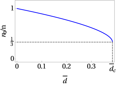
Figure 1: (Color online) Condensate fraction $n_{0}/n$ as function of dimensionless disorder strength $\overline{d}$.

Now we check whether our results are compatible with the Huang-Meng theory HM-1 ; HM-3 ; HM-4 ; HM-5 ; HM-2 , where the Bose-glass order parameter of a homogeneous dilute Bose gas at zero temperature in case of weak disorder regime is deduced within the seminal Bogoliubov theory. The Bose-glass order parameter in three dimensions via the Huang-Meng theory is proportional to the disorder strength and yields in dimensionless form:

$$\frac{q_{{\rm HM}}}{\sqrt{n/g}}=\frac{\overline{d}}{\sqrt{2}}.$$ (14)

In our Hartree-Fock mean-field theory the Bose-glass order parameter in case of weak disorder strength turns out to be

$$\frac{q_{w}}{\sqrt{n/g}}=\overline{d}.$$ (15)

Thus, our theory agrees with the Huang-Meng theory at least qualitatively. But quantitatively the comparison of Eqs. (14) and (15) reveals that a factor of $\sqrt{2}$ is missing in our result (15). This is due to the fact that the Hartree-Fock theory does not contain the Bogoliubov channel, which is included in the Huang-Meng theory.

According to Ref. Navez , the disorder strength value corresponding to the quantum phase transition is $\overline{d}_{{\rm{c}}}=0.53$. Thus, our quantum phase transition disorder value $\overline{d}_{{\rm{c}}}=0.384$ is of the same order as the one in Ref. Navez , but again we miss a factor of $\sqrt{2}$ in our result. In the one-dimensional case, as discussed in Ref. Paper1 , a factor $2^{3/2}$ is missing, while in the three-dimensional case the discrepancy only amounts to a factor of $\sqrt{2}$, so we conclude that our Hartree-Fock theory is more compatible with the literature in higher dimensions than in lower ones.

Furthermore, we compare the critical value of the disorder strength $\overline{d}_{{\rm{c}}}$ with the non-perturbative approach of Refs. Nattermann ; Natterman2 , which starts from the Bose-glass phase and goes towards the superfluid phase for decreasing disorder strength. By investigating energetically shape and size of the local minicondensates in the disorder landscape, the quantum phase transition is predicted to occur at the disorder strength value $\tilde{d}=\sqrt{\frac{3}{8\pi}}\simeq 0.345$, which is again of the same order as our $\tilde{d}_{{\rm c}}$.

III.2 Thomas-Fermi approximation

We deal now with the trapped case. The exact analytical solution of the differential equation (6) is impossible to obtain even in the absence of disorder. Therefore, we approximate its solution via the Thomas-Fermi (TF) approximation, which is based on neglecting the kinetic energy.

It turns out that we have to distinguish between two different spatial regions: the superfluid region, where the bosons are distributed in the condensate as well as in the minima of the disorder potential, and the Bose-glass region, where there are no bosons in the global condensate and all bosons contribute only to the local Bose-Einstein condensates. In the following the radius of the superfluid region, i.e., the condensate radius, is denoted by $R_{{\rm{TF1}}}$, while the radius of the whole bosonic cloud $R_{{\rm{TF2}}}$ is called the cloud radius.

Within the TF approximation the algebraic equations (7) and (9) remain the same, but the differential equation (6) reduces to an algebraic relation in the superfluid region:

$$gn{}_{0}(r)=\left[\sqrt{-\mu+d^{2}+2gn(r)+V(r)}+d\right]^{2}.$$ (16)

Outside the superfluid region, i.e., in the Bose-glass region, Eq. (6) reduces simply to $n{}_{0}(r)=0$. The advantage of the TF approximation is that now we have only three coupled algebraic equations.

At first we consider the superfluid region. Equations (7), (9), and (16) reduce in the superfluid region to:

$$\tilde{n}_{0}\left(\tilde{r}\right)=\left[\sqrt{-\tilde{\mu}+2\tilde{n}(\tilde{r})+\tilde{r}^{2}}+\tilde{d}\right]^{2},$$ (17)

$$\tilde{q}\left(\tilde{r}\right)=\frac{\tilde{d}\left[\sqrt{-\tilde{\mu}+2\tilde{n}(\tilde{r})+\tilde{r}^{2}}+\tilde{d}\right]^{2}}{\sqrt{-\tilde{\mu}+2\tilde{n}(\tilde{r})+\tilde{r}^{2}}},$$ (18)

$$\tilde{n}\left(\tilde{r}\right)=\frac{\left[\sqrt{-\tilde{\mu}+2\tilde{n}(\tilde{r})+\tilde{r}^{2}}+\tilde{d}\right]^{3}}{\sqrt{-\tilde{\mu}+2\tilde{n}(\tilde{r})+\tilde{r}^{2}}},$$ (19)

where $\tilde{n}_{0}(\tilde{r})=n_{0}(r)/\overline{n},$ $\tilde{q}(\tilde{r})=q(r)/\overline{n}$, and $\tilde{n}(\tilde{r})=n(r)/\overline{n}$ denote the dimensionless condensate density, Bose-glass order parameter, and total density, respectively. Furthermore, we have introduced the dimensionless radial coordinate $\tilde{r}=r/R_{{\rm{TF}}}$, the dimensionless chemical potential $\tilde{\mu}=(\mu-d^{2})/\bar{\mu}$, the dimensionless disorder strength $\tilde{d}=\frac{\xi}{\mathcal{L}}$, the coherence length in the center of the trap $\xi=\frac{l^{2}}{R_{{\rm{TF}}}}$, the oscillator length $l=\sqrt{\frac{\hbar}{M\Omega}}$, the maximal total density in the clean case $\overline{n}=\bar{\mu}/g$, and the TF cloud radius $R_{{\rm{TF}}}=l\sqrt{2\bar{\mu}/\hbar\Omega}$. The chemical potential in the absence of the disorder $\bar{\mu}=\frac{15^{2/5}}{2}\Big{(}\frac{aN}{l}\Big{)}^{2/5}\hslash\Omega$ serves here as the underlying energy scale and is deduced from the normalization condition (5) in the clean case, i.e., for $d=0$.

Equation (19) is of the third order with respect to the expression $\sqrt{-\tilde{\mu}+2\tilde{n}(\tilde{r})+\tilde{r}^{2}}$, therefore, we use the Cardan method to solve it analytically Greiner . We determine the condensate radius $\tilde{R}_{{\rm TF1}}$ at the coordinate where the solution of (19) for the total density stops to exist, then select the smallest solution, which corresponds to $\tilde{R}_{{\rm TF1}}=\sqrt{\tilde{\mu}-3\tilde{d}^{2}-6\sqrt{3}\tilde{d}^{2}\cos\left(\frac{\pi}{18}\right)}$. Now we have just to insert the obtained particle density $\tilde{n}(\tilde{r})$ into the two other equations $(\ref{15})$ and $(\ref{16})$ in order to get both the condensate density $\tilde{n}_{0}(\tilde{r})$ and the Bose-glass order parameter $\tilde{q}(\tilde{r})$, respectively.

In the Bose-glass region the condensate vanishes, i.e., $\tilde{n}_{0}(\tilde{r})=0$ and $\tilde{n}(\tilde{r})=\tilde{q}(\tilde{r})$, and the self-consistency equation (7) reduces to:

$$\tilde{q}(\tilde{r})=\frac{\tilde{\mu}-\tilde{r}^{2}}{2}.$$ (20)

This Bose-glass region ends at the cloud radius $\tilde{R}_{{\rm TF2}}=\sqrt{\tilde{\mu}}$. We also need to write down the dimensionless equivalent of the normalization condition (5), which reads:

$$\int_{0}^{\tilde{R}_{{\rm{TF2}}}}\tilde{n}(\tilde{r})\tilde{r}^{2}d\tilde{r}=\frac{2}{15},$$ (21)

where the total density $\tilde{n}(\tilde{r})$ in equation (21) is the combination of the total densities from both the superfluid region and the Bose-glass region. The purpose of Eq. (21) is to determine the dimensionless chemical potential $\tilde{\mu}$ from the respective system parameters.

III.3 Thomas-Fermi results

Before choosing any parameters for the BEC system, we have to justify using the TF approximation and determine its range of validity. To this end we rewrite Eq. (6) in the clean case, where the total density coincides with the condensate one:

$$\left[-1+\tilde{n}(\tilde{r})+\tilde{r}^{2}-\left(\frac{\xi}{R_{{\rm{TF}}}}\right)^{2}\frac{1}{\tilde{r}^{2}}\frac{\partial}{\partial\tilde{r}}\left(\tilde{r}^{2}\frac{\partial}{\partial\tilde{r}}\right)\right]\,$$

$$\!\!\!\!\!\!\!\!\!\!\!\!\!\!\!\!\!\!\!\!\!\!\!\!\!\!\!\!\!\!\!\!\!\!\!\!\times\sqrt{\tilde{n}\left(\tilde{r}\right)}=0.$$ (22)

We read off from Eq. (22) that the TF approximation is only justified when $\xi\ll R_{{\rm{TF}}}$.

In this subsection we perform our study for ${}^{87}{\rm{Rb}}$ atoms and for the following experimentally realistic parameters: $N=10^{6}$, $\Omega=2\pi\times 100{\rm\,{Hz}}$, and $a=5.29\,{\rm{nm}}$. For those parameters the oscillator length reads $l=1.08{\rm\,{\mu m}},$ the coherence length turns out to be $\xi=115\,{\rm{nm}},$ and the Thomas-Fermi radius is given by $R_{{\rm{TF}}}=10.21{\rm\,{\mu m}}$. Thus the assumption $\xi\ll R_{{\rm{TF}}}$ for the TF approximation is, indeed, fulfilled.

Using those parameter values we solve in the superfluid region Eq. (19) for the total density and insert the result into Eqs. (17) and (18) to get the condensate density and the Bose-glass order parameter, respectively. This has to be combined with Eq. (20) for the Bose-glass region. After that we fix the chemical potential $\tilde{\mu}$ using the normalization condition (21). The resulting densities are combined and plotted in Fig. 3a for the disorder strength $\tilde{d}=0.175$.

Figure 3a reveals that, at the condensate radius $\tilde{R}_{{\rm TF1}}$, a downward jump of the condensate density $\tilde{n}_{0}(\tilde{r})$, and an upward jump of the Bose-glass order parameter $\tilde{q}(\tilde{r})$ occur in such a way that the total density $\tilde{n}(\tilde{r})$ remains continuous but reveals a discontinuity of the first derivative. In the Bose-glass region both the total density and the Bose-glass parameter coincide and decrease until vanishing at the cloud radius $\tilde{R}_{{\rm TF2}}$. The TF approximation captures the properties of the system in both the superfluid and the Bose-glass region but not in the transition region. This is an artifact of the applied TF approximation.

The ratio of the condensate density at the condensate radius $\tilde{n}_{0}(\tilde{R}_{{\rm TF1}})$ with respect to the condensate density at the center of the BEC $\tilde{n}_{0}(0)$ in Fig. 3b reveals for which range of the disorder strength the TF approximation is valid. As only a moderate density jump of about 50% should be reasonable, our approach is restricted to a dis-

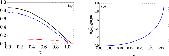
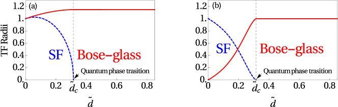
Figure 2: (Color online) (a) Total density $\tilde{n}(\tilde{r})$ (solid, black), condensate density $\tilde{n}_{0}(\tilde{r})$ (dotted, blue), Bose-glass order parameter $\tilde{q}(\tilde{r})$ (dotted-dashed, red) as a function of radial coordinate $\tilde{r}$ for the disorder strength $\tilde{d}=0.175$ both for superfluid region and Bose-glass region. (b) Ratio of $\tilde{n}_{0}(\tilde{R}_{{\rm TF1}})$ and $\tilde{n}_{0}(0)$ as a function of disorder strength $\tilde{d}$.

Figure 3: (Color online) (a) Condensate radius (dashed, blue) and cloud radius (solid, red) and (b) fractional number of condensed particles $N_{0}/N$ (dashed, blue) and in the disconnected local minicondensates $Q/N$ (solid, red), as a function of disorder strength $\tilde{d}$.

order strength of about $\tilde{d}\simeq 0.3$. For a larger disorder strength $\tilde{d}$ one would have to go beyond the TF approximation and take the influence of the kinetic energy in Eq. (6) into account.

The resulting Thomas-Fermi radii are plotted in Fig. 3a. When the disorder strength increases, the condensate radius at first increases slightly, then decreases until it vanishes, which corresponds to a quantum phase transition at $\tilde{d}_{{\rm c}}=\frac{2^{1/5}}{\sqrt{3+6\sqrt{3}\cos\frac{\pi}{18}}}\backsimeq 0.315$. This critical value of the disorder strength is obtained by setting the cloud radius $\tilde{R}_{{\rm TF1}}$ to zero. Thus, superfluidity is destroyed in our model at a critical disorder strength $\tilde{d}_{{\rm c}}$, where approximately our TF approximation breaks down. Now we compare this critical value of the disorder strength with the one obtained in Refs. Nattermann ; Natterman2 , where a non-perturbative approach is used, which investigates energetically shape and size of the local minicondensates in the disorder landscape. Thus, it is determined for a decreasing disorder strength once the Bose-glass phase becomes unstable and goes over in the superfluid phase. In those references the quantum phase transition for our system parameters is predicted to occur at the disorder strength value $\tilde{d}=0.115$, which is of the same order as our $\tilde{d}_{{\rm c}}$.

Contrary to the condensate radius, the cloud radius increases monotonously with the disorder strength and eventually saturates, so that in the strong disorder regime the bosonic cloud reaches its maximal radius of $\underset{\tilde{d}\rightarrow\infty}{{\rm lim}}$ $\tilde{R}_{{\rm TF2}}=2^{1/5}\backsimeq 1.148$, which is obtained by inserting the Bose-glass region density (20) into the normalization condition (21).

The same conclusion can be read off from Fig. 3b, where the fractional number of the condensate defined via $N_{0}/N=\frac{15}{2}\int_{0}^{\tilde{R}_{{\rm{TF1}}}}\tilde{r}^{2}\tilde{n}_{0}\left(\tilde{r}\right)d\tilde{r}$ is plotted. We note that $N_{0}/N$ is equal to one in the clean case, i.e., all particles are in the condensate, then it decreases with the disorder strength until it vanishes at $\tilde{d}_{{\rm{c}}}$, marking the end of the superfluid phase and the beginning of the Bose-glass phase. Conversely, the fraction of atoms in the disconnected minicondensates $Q/N=\frac{15}{2}\int_{0}^{R_{{\rm{TF2}}}}\tilde{r}^{2}\tilde{q}\left(\tilde{r}\right)d\tilde{r}$ increases with the disorder strength until it reaches its maximum at $\tilde{d}_{{\rm{c}}}$. Then it remains constant and equals to one in the Bose-glass phase, since all particles are localized in the respective minima of the disorder potential.

From Fig. 3b we conclude that the TF approximation is valid only in the weak disorder regime, but it is not a good approximation for intermediate or strong disorder. The TF approximation has a larger range of validity with respect to the disorder strength in three dimensions than in one dimension treated in Ref. Paper1 due to the fact that the fluctuations are more violent in lower dimensions. In order to have a global picture, not only in the presence of weak disorder but also in the presence of intermediate and strong one, we use in the following subsection another approximation method to treat the dirty boson problem: the variational approach.

III.4 Variational method

Since the three self-consistency Eqs. (6), (7), and (9), as well as Eq. (4) are obtained by extremising the free energy (3), we can apply the variational method in the spirit of Refs. Kleinert1 ; Kleinert2 ; Var1 ; Var2 to obtain approximate results. In order to be able to compare the variational results with the analytical ones obtained in the previous subsection, we use the same rescaling parameters already introduced below Eq. (19) for all functions and parameters. To this end, we have to multiply Eq. (3) with the factor $1/\left(\bar{\mu}\overline{n}R_{{\rm{TF}}}^{3}\right)$ to obtain:

$$\tilde{\mathcal{F}} =4\pi\int_{0}^{\infty}d\tilde{r}\tilde{r}^{2}\left\{-\left[\tilde{q}\left(\tilde{r}\right)+\tilde{n}_{0}\left(\tilde{r}\right)\right]^{2}-\frac{1}{2}\tilde{n}_{0}^{2}\left(\tilde{r}\right)\right.$$

$$+\tilde{d}\tilde{Q}_{0}(\tilde{r})\left[\tilde{q}\left(\tilde{r}\right)+\tilde{n}_{0}\left(\tilde{r}\right)\right]-\sqrt{\tilde{n}_{0}\left(\tilde{r}\right)}\Biggl{\{}\tilde{\tilde{\mu}}+\tilde{d}\tilde{Q}_{0}(\tilde{r})$$

$$-2\left[\tilde{q}\left(\tilde{r}\right)+\tilde{n}_{0}\left(\tilde{r}\right)\right]-\tilde{r}^{2}+\left(\frac{\xi}{R_{{\rm{TF}}}}\right)^{2}\frac{1}{\tilde{r}^{2}}\frac{\partial}{\partial\tilde{r}}\left(\tilde{r}^{2}\frac{\partial}{\partial\tilde{r}}\right)\Biggr{\}}$$

$$\times\sqrt{\tilde{n}_{0}\left(\tilde{r}\right)}-2\tilde{d}\left[\tilde{q}\left(\tilde{r}\right)+\tilde{n}_{0}\left(\tilde{r}\right)\right]$$

$$\left.\times\sqrt{-\tilde{\mu}^{\prime}+2\left[\tilde{q}\left(\tilde{r}\right)+\tilde{n}_{0}\left(\tilde{r}\right)\right]+\tilde{r}^{2}-2\tilde{d}\tilde{Q}_{0}(\tilde{r})}\right\},$$ (23)

where we have introduced the dimensionless free energy $\tilde{\mathcal{F}}=\mathcal{F}/\left(\bar{\mu}\overline{n}R_{{\rm{TF}}}^{3}\right)$, the dimensionless chemical potential $\tilde{\mu}^{\prime}=\mu/\bar{\mu}$, and the dimensionless auxiliary function $\tilde{Q}_{0}(\tilde{r})=\frac{1}{\hbar\sqrt{\pi\bar{\mu}}}\left(\frac{2\pi\hbar^{2}}{M}\right)^{3/2}Q_{0}(r)$.

Motivated by the analytical results presented in Fig. 3a, we use the following three ansatz expressions for the condensate density $\tilde{n}_{0}\left(\tilde{r}\right)$, the Bose-glass order parameter $\tilde{q}\left(\tilde{r}\right)$, and the auxiliary function $\tilde{Q}_{0}(\tilde{r})$:

$$\tilde{n}_{0}\left(\tilde{r}\right)=\alpha e^{-\sigma\tilde{r}^{2}},$$ (24)

$$\tilde{q}\left(\tilde{r}\right)+\tilde{n}_{0}\left(\tilde{r}\right)=\gamma e^{-\theta\tilde{r}^{2}},$$ (25)

$$\tilde{Q}_{0}(\tilde{r})=2\frac{\tilde{q}\left(\tilde{r}\right)+\tilde{n}_{0}\left(\tilde{r}\right)}{\tilde{d}}-\left(\zeta+\eta\tilde{r}^{2}\right),$$ (26)

where $\alpha$, $\sigma$, $\gamma$, $\theta$, $\zeta$, and $\eta$ denote the respective variational parameters. The parameters $\alpha$ and $\gamma$ are proportional to the number of particles in the condensate and the total number of particles, while the parameters $\sigma$ and $\theta$ represent the width of the condensate density and the total density, respectively. Inserting the ansatz (24)–(26) into the free energy (23) and performing the integral yields:

$$\tilde{\mathcal{F}} = \pi^{3/2}\left\{\frac{\sqrt{2}\gamma^{2}}{4\theta^{3/2}}+3\frac{\alpha}{2\sigma^{5/2}}-\frac{\alpha}{8\sigma^{3/2}}\left(8\tilde{\mu}^{\prime}+\sqrt{2}\alpha\right)\right.$$ (27)

$$\!\!\!\!\!\!\!\!\!\!\!\!\!\!\!\!\!\!+\left(\frac{\xi}{R_{{\rm{TF}}}}\right)^{2}\frac{3\alpha}{2\sqrt{\sigma}}\left.+\tilde{d}\left(\frac{\alpha\zeta}{\sigma^{3/2}}+\frac{3\alpha\eta}{2\sigma^{5/2}}-\frac{\gamma\left(3\eta+2\zeta\theta\right)}{2\theta^{5/2}}\right)\right\}$$

$$\!\!\!\!\!\!\!\!\!\!\!\!\!\!\!\!\!\!+\frac{2\pi\tilde{d}\gamma\left(\tilde{d}\zeta-\tilde{\mu}^{\prime}\right)}{\theta\sqrt{1+\tilde{d}\eta}}e^{\frac{\tilde{d}\zeta-\tilde{\mu}^{\prime}}{2+2\tilde{d}\eta}\theta}K_{1}\left(\frac{\tilde{d}\zeta-\tilde{\mu}^{\prime}}{2+2\tilde{d}\eta}\theta\right),$$

where $K_{1}\left(s\right)$ represents the modified Bessel function of second kind.

The free energy (27) has now to be extremised with respect to the variational parameters $\alpha$, $\sigma$, $\gamma$, $\theta$, $\zeta$, and $\eta$. Together with the thermodynamic condition $-\frac{\partial\tilde{\mathcal{F}}}{\partial\tilde{\mu}^{\prime}}=\frac{4}{3}$, we have seven coupled algebraic equations for seven variables $\alpha$, $\sigma$, $\gamma$, $\theta$, $\zeta$, $\eta$, and $\tilde{\mu}^{\prime}$ that we solve numerically.

From all possible solutions we select the physical one with the smallest free energy, then we insert the resulting variational parameters $\alpha$, $\sigma$, $\gamma$, and $\theta$ into the variational ansatz (24) and (25) in order to get the variational total density $\tilde{n}(\tilde{r})$, the variational condensate density $\tilde{n}_{0}(\tilde{r})$, and the variational Bose-glass order parameter $\tilde{q}(\tilde{r})$.

In Fig. 6a the total density $\tilde{n}(\tilde{r})$ has a Gaussian shape and vanishes at the cloud radius $\tilde{R}_{{\rm{TF2}}}$. The maximal value of the total density decreases with the disorder strength. The condensate density $\tilde{n}_{0}(\tilde{r})$ in Fig. 6b has a similar qualitative behavior as the total density and vanishes at the condensate radius $\tilde{R}_{{\rm{TF1}}}$. The maximal value of the condensate density decreases also with the disorder strength. The response of the condensate density to disorder can be clearly seen in Fig. 6b, where the fractional number of condensed particles $N_{0}/N$ is plotted as a function of the disorder strength. In the clean case all particles are in the condensate, but, when we increase the disorder strength, more and more particles leave the condensate until the condensate vanishes at the critical disorder strength $\tilde{d}_{{\rm{c}}}=0.5183$.

The Bose-glass order parameter $\tilde{q}(\tilde{r})$ in Fig. 6c has a similar shape as the two previous densities $\tilde{n}(\tilde{r})$ and $\tilde{n}_{0}(\tilde{r})$. However, when we increase the disorder strength, the maximal value of the Bose-glass order parameter also increases. A better understanding of the effect of the dis-

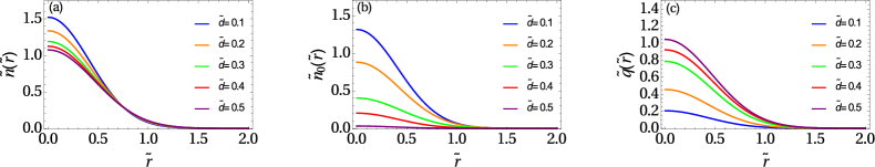
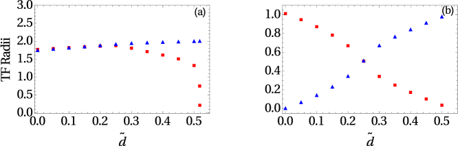
Figure 4: (Color online) Spatial distribution of: (a) particle density $\tilde{n}(\tilde{r})$, (b) condensate density $\tilde{n}_{0}(\tilde{r})$, and (c) Bose-glass order parameter $\tilde{q}(\tilde{r})$ for increasing disorder strength $\tilde{d}$, from the top to the bottom in the center in (a) and (b), and from the bottom to the top in (c).

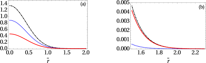
Figure 5: (Color online) (a) Cloud radius $\tilde{R}_{{\rm{TF2}}}$ (triangle, blue) and condensate radius $\tilde{R}_{{\rm{TF1}}}$ (square, red) and (b) fractional number of condensed particles $N_{0}/N$ (square, red) and fractional number of particles $Q/N$ in the disconnected local mini-condensates (triangle, blue) as function of disorder strength $\tilde{d}$.

Figure 6: (Color online) Spatial distribution of: (a) particle density $\tilde{n}(\tilde{r})$ (dotted-dashed, black), condensate density $\tilde{n}_{0}(\tilde{r})$ (dotted, blue), Bose-glass order parameter $\tilde{q}(\tilde{r})$ (solid, red) and (b) blow-up of border region for $\tilde{d}=0.35$.

order on the local minicondensates can be deduced from Fig. 6b, where the fractional number of particles $Q/N$ in the disconnected local minicondensates is zero in the clean case and then increases with the disorder strength until reaching the maximal value of one. This means that more and more bosons go into the local minima of the disorder potential when we increase the disorder strength. At the critical disorder strength $\tilde{d}_{{\rm{c}}}=0.518$ all particles are in the minicondensates.

In order to know whether the bosonic cloud contains beside the superfluid region also a Bose-glass region, we plot the total density $\tilde{n}(\tilde{r})$, the condensate density $\tilde{n}_{0}(\tilde{r})$, and the Bose-glass order parameter $\tilde{q}(\tilde{r})$ together in Fig. 6a for the disorder strength value $\tilde{d}=0.35$. The blow-up of the border region in Fig. 6b shows clearly that the condensate density vanishes, while the Bose-glass order parameter still persists, which is the definition of the Bose-glass region. The cloud radius $\tilde{R}_{{\rm{TF2}}}$ and the condensate radius $\tilde{R}_{{\rm{TF1}}}$ are conveniently defined by the length, where the total density and the condensate density are equal to $10^{-4}$, respectively. Both radii are increasing with the disorder strength in the weak disorder regime in Fig. 6a. In the intermediate disorder regime, the cloud radius keeps increasing monotonously with the disorder strength, while the condensate radius vanishes at the critical disorder value $\tilde{d}_{{\rm{c}}}=0.518$, which marks the location of a quantum phase transition. For higher disorder strengths $\tilde{d}>\tilde{d}_{{\rm{c}}}$ the variational treatment breaks down as it turns out to have negative solutions for the condensate density. So with this method it is not possible to determine if, for stronger disorder, the cloud radius keeps increasing or remains constant.

III.5 Comparison between TF approximation and variational results

Now we compare the physical quantities obtained via the two different methods, the TF approximation and the variational approach. We start with the densities: the total density $\tilde{n}(\tilde{r})$, the condensate density $\tilde{n}_{0}(\tilde{r})$, and the Bose-glass order parameter $\tilde{q}(\tilde{r})$ are plotted for the disorder strength value $\tilde{d}=0.2$ in Fig. 8. We know already from treating the one-dimensional dirty boson problem in Ref. Paper1 , where we also performed extensive numerical simulations, that the TF approximation describes well the weak disorder regime, while the variational method is more accurate to describe the intermediate disorder regime. Based on this conclusion our comparison is here more a qualitative than a quantitative one. The total densities $\tilde{n}(\tilde{r})$ in Fig. 8a agree qualitatively well. The same can be said for the condensate density $\tilde{n}_{0}(\tilde{r})$ in Fig. 8b, except from the jump in the TF-approximated condensate density. For the Bose-glass order parameter $\tilde{q}(\tilde{r})$ in Fig. 8c we read off that the TF approximation for the density of the bosons in the local minima of the disorder potential is maximal at the border of the trap, but according to the variational result this density is maximal in the center of the trap.

The TF-approximated and the variational Thomas-Fermi radii are compared in Fig. 8. In Fig. 8a the variational and the TF-approximated condensate radius $\tilde{R}_{{\rm{TF1}}}$ have the same qualitative behavior, both increase first barely with the disorder strength $\tilde{d}$ in the weak disorder regime, then decrease with it in the intermediate disorder regime until they vanish at the quantum phase transition. Thus, both analytically and variationaly obtained condensate radii $\tilde{R}_{{\rm{TF1}}}$ indicate the existence of a quantum phase transition, but at two different values of the disorder strength, namely $\tilde{d}_{{\rm{c}}}=0.315$ and $\tilde{d}_{{\rm{c}}}=0.5183$, respectively. The variational quantum phase transition happens at a larger disorder strength than the TF-approximated one. Figure 8b shows that in the weak disorder regime, both the variational and the analytical cloud radii $\tilde{R}_{{\rm{TF2}}}$ increase with the disorder strength. In the intermediate disorder regime the analytical cloud radius remains constant, while the variational one keeps increasing with the disorder strength. Due to the lack of information about determine higher disorder strengths $\tilde{d}$, we can not know if the variational cloud radius keeps increasing even further or remains constant.

From the discussion above we conclude that the TF approximation and the variational method are producing similar qualitative results, contrarily to the one-dimensional case in Ref. Paper1 , where the TF-approximated and the variational results disagree completely. From studying the one-dimensional dirty boson problem in Ref. Paper1 , we can say that the TF approximation produces satisfying results in the weak disorder regime, while the variational method within the ansatz (24)–(26) is a good approximation to describe the BEC system in the intermediate disorder regime and has the advantage of being able to describe the border of the cloud, where the Bose-glass region is situated and where the TF approximation fails. Although the variational method does not provide physical results for larger disorder strengths, its combination together with the TF approximation for the weak disorder regime covers a significant range of disorder strengths.

IV 3D Dirty Bosons at Finite Temperature

In this section we consider the three-dimensional dirty BEC system to be at finite temperature, so that also the thermal density $n_{{\rm th}}\left(r\right)$ has to be taken into account. After starting with the homogeneous dirty boson problem, we restrict ourselves first to the trapped clean case, then we treat the trapped disordered one, both in TF approximation, where we work out the different densities as well as the respective Thomas-Fermi radii. This allows us to study the impact of both temperature and disorder on the distribution of the densities as well as the Thomas-Fermi radii.

IV.1 Homogeneous case

We start with revisiting the homogeneous case, which was already studied in Ref. Intro-90 , since it is the simplest one. Here we have $V(r)=0$ and Eqs.  (6)–(9) reduce in the superfluid phase to:

$$gn{}_{0}=\left[\sqrt{-\mu+d^{2}+2gn}+d\right]^{2},$$ (28)

$$q=\frac{dn{}_{0}}{\sqrt{-\mu+d^{2}+2gn}},$$ (29)

$$n_{{\rm th}}=\left(\frac{M}{2\pi\beta\hslash^{2}}\right)^{3/2}\varsigma_{\ 3/2}\left(e^{\beta\ \left(\mu-d^{2}-2gn\right)}\right),$$ (30)

$$n=n_{0}+q+n_{{\rm th}}.$$ (31)

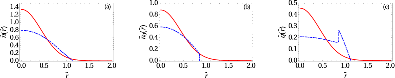
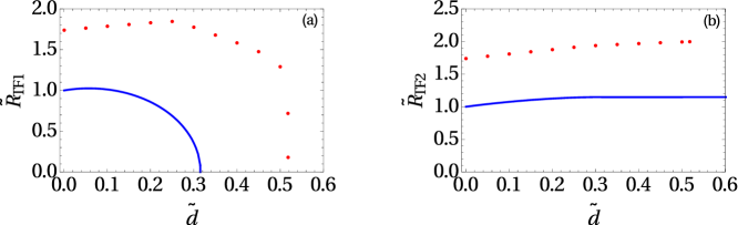
Figure 7: (Color online) Spatial distribution of (a) total particle density $\tilde{n}(\tilde{r})$, (b) condensate density $\tilde{n}_{0}(\tilde{r})$, and (c) Bose-glass order parameter $\tilde{q}(\tilde{r})$: variational (solid, red), and analytical (dotted, blue) for $\tilde{d}=0.2$.

Figure 8: (Color online) Analytical (solid, blue) and variational (dotted, red) results for (a) condensate radius $\tilde{R}_{{\rm{TF1}}}$ and (b) cloud radius $\tilde{R}_{{\rm{TF2}}}$, as functions of disorder strength $\tilde{d}$.

Note that we drop in this subsection again the spatial dependence of all densities due to the homogeneity. From Eqs. (28)–(31) we get the following algebraic equation for the condensate fraction $n{}_{0}/n$:

$$\left(\frac{n_{0}}{n}\right)^{3/2}-\sqrt{\frac{n_{0}}{n}}+\overline{d}+\left(\frac{T}{\varsigma\left(\frac{3}{2}\right)^{2/3}T_{{\rm{c}}}^{0}}\right)^{3/2}\left(\sqrt{\frac{n_{0}}{n}}-\overline{d}\right)$$

$$\times\varsigma_{\ 3/2}\left(e^{-2\frac{T_{{\rm{c}}}^{0}}{T}\varsigma\left(\frac{3}{2}\right)^{2/3}\gamma^{1/3}\ \left[\sqrt{\frac{n_{0}}{n}}-\overline{d}\right]^{2}}\right)=0.$$ (32)

Here $\overline{d}=\frac{\xi}{\mathcal{L}}$ denotes the dimensionless disorder strength, $\gamma=na^{3}$ the gas parameter, and $T_{{\rm{c}}}^{0}=\frac{2\pi\hslash^{2}}{Mk_{B}}\left(\frac{n}{\varsigma\left(\frac{3}{2}\right)}\right)^{2/3}$ the critical temperature of the ideal Bose gas, where again $\xi=\frac{\hbar}{\sqrt{2Mgn}}$ stands for the coherence length and $\mathcal{L}=\frac{2\pi\hbar^{4}}{M^{2}D}$ represents the Larkin length Nattermann ; Larkin . Note that at zero temperature Eq. (32) reduces to Eq. (13). Figure 9 shows that the condensate fraction generically decreases with increasing disorder strength $\overline{d}$. Furthermore, our Hartree-Fock mean-field theory predicts that the condensate density stops to exist at a critical value $\overline{d}_{{\rm{c}}}$. We interpret this as a sign that a phase transition occurs in the homogeneous BEC from the superfluid to the Bose-glass phase. If we compare in Fig. 9 the dotted blue line, which corresponds to a finite temperature, with the solid red line, which corresponds to the zero-temperature case of Subsection III.A, we observe that $\overline{d}_{{\rm{c_{1}}}}\simeq 0.30<\overline{d}_{{\rm{c_{3}}}}\simeq 0.384$ and conclude that the critical disorder strength $\overline{d}_{{\rm{c}}}$ decreases with increasing temperature $T$. Comparing at fixed temperature the dotted blue line for a weakly interacting ${}^{87}{\rm{Rb}}$ gas, which corresponds to the gas parameter of about $\gamma=0.0007$ according to Ref. Weak-Interaction-Stringari , with the dotted-dashed green line for a strongly interacting ${}^{4}{\rm{He}}$, which corresponds to the gas parameter of about $\gamma=0.2366$ according to Ref. Strong-Interaction-Pathria , yields that $\overline{d}_{{\rm{c_{1}}}}\simeq 0.30<\overline{d}_{{\rm{c_{2}}}}\simeq 0.331$. But in order to draw a conclusion how the gas parameter $\gamma$ affects the critical disorder strength, one has to take into account that it is included in the definition of the dimensionless disorder strength $\overline{d}=\frac{d}{\sqrt{gn}}$. With this, we conclude $d_{{\rm{c_{1}}}}>d_{{\rm{c_{2}}}}$, i.e., the critical disorder strength $d_{{\rm{c}}}$ decreases with increasing the gas parameter $\gamma$. These findings suggest that a corresponding phase transition will also appear in the trapped case, which is studied later on in Subsection IV.G.

To illustrate our results further, we determine where the superfluid, the Bose-glass, and the thermal phase exist within the phase diagram, which is spanned by the temperature and the disorder strength. Whereas this phase diagram was sketched qualitatively in Ref. Intro-90 , we determine it here quantitatively in Fig. 10. This phase diagram follows from solving Eq. (32) together with setting its derivative with respect to $n_{0}/n$ to zero, i.e.,

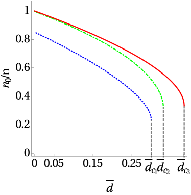
Figure 9: (Color online) Condensate fraction $n_{0}/n$ as function of dimensionless disorder strength $\overline{d}$ for $\gamma=0.0007$ and $T/T_{{\rm{c}}}^{0}=0.6$ (dotted, blue), $\gamma=0.2366$ and $T/T_{{\rm{c}}}^{0}=0.6$ (dotted-dashed, green), and $T=0$ (solid, red).

$$\frac{3}{2}\sqrt{\frac{n_{0}}{n}}-\frac{1}{2\sqrt{n_{0}/n}}+\frac{1}{2\sqrt{n_{0}/n}}\left(\frac{T}{\varsigma\left(\frac{3}{2}\right)^{2/3}T_{{\rm{c}}}^{0}}\right)^{3/2}$$

$$\times\varsigma_{\ 3/2}\left(e^{-2\frac{T_{{\rm{c}}}^{0}}{T}\varsigma\left(\frac{3}{2}\right)^{2/3}\gamma^{1/3}\ \left[\sqrt{\frac{n_{0}}{n}}-\overline{d}\right]^{2}}\right)-\frac{2\gamma^{1/3}}{\sqrt{n_{0}/n}}$$

$$\times\sqrt{\frac{T}{\varsigma\left(\frac{3}{2}\right)^{2/3}T_{{\rm{c}}}^{0}}}\left(\sqrt{\frac{n_{0}}{n}}-\overline{d}\right)^{2}$$

$$\times\varsigma_{\ 1/2}\left(e^{-2\frac{T_{{\rm{c}}}^{0}}{T}\varsigma\left(\frac{3}{2}\right)^{2/3}\gamma^{1/3}\ \left[\sqrt{\frac{n_{0}}{n}}-\overline{d}\right]^{2}}\right)=0.$$ (33)

The phase diagram in Fig. 10a corresponds to a weakly interacting ${}^{87}{\rm{Rb}}$ gas, while the phase diagram in Fig. 10b corresponds to a strongly interacting ${}^{4}{\rm{He}}$ gas. The critical disorder strength $\overline{d}_{{\rm{c}}}$ decreases with the temperature $T$. In the clean case $\overline{d}=0$ there is a critical temperature $T_{{\rm{c}}}$ at which the superfluid, which is stable for $T<T_{{\rm{c}}}$, goes over into the thermal Bose-gas, which is stable for $T>T_{{\rm{c}}}$. Note that, due to the weak repulsive interaction, this critical temperature $T_{{\rm{c}}}$ turns out to be larger than the critical temperature of the ideal Bose gas $T_{{\rm{c}}}^{0}$ by about

$$\Delta T_{{\rm{c}}} =T_{{\rm{c}}}-T_{{\rm{c}}}^{0}\simeq 1.3\,\gamma^{1/3}T_{{\rm{c}}}^{0}.$$ (34)

Note that the result (34) is non-trivial as it involves a resummation of an infrared divergent perturbation series, which has been worked out on the basis of variational perturbation theory in Refs. 5-loops-kleinert ; Boris , and has been confirmed by extensive MC simulations Prokof . For the weakly interacting Bose gas in Fig. 10a $T_{{\rm{c}}}/T_{{\rm{c}}}^{0}=1.103$, which agrees well with the result obtained by using formula (34), where we get $T_{{\rm{c}}}/T_{{\rm{c}}}^{0}\simeq 1.115$. The same can be remarked for the strongly interacting Bose gas in Fig. 10b, where $T_{{\rm{c}}}/T_{{\rm{c}}}^{0}=1.65$, which agrees well with the result obtained by using formula (34) $T_{{\rm{c}}}/T_{{\rm{c}}}^{0}\simeq 1.796$. Furthermore, there is a triple point $\overline{d}_{{\rm{T}}}$, where the three phases coexist and at which $T=T_{{\rm{c}}}^{0}$ and $\mu_{c}=2gn=2g\left(\frac{Mk_{B}T_{{\rm{c}}}^{0}}{2\pi\hslash^{2}}\right)^{3/2}\varsigma\left(\frac{3}{2}\right)$. So $T_{{\rm{c}}}^{0}$ of the ideal Bose gas turns out to be in our context the critical temperature for the appearance of the Bose-glass phase. For $\gamma=0.0007$ we have $\overline{d}_{{\rm{T}}}=0.111$, while for $\gamma=0.2366$ we obtain $\overline{d}_{{\rm{T}}}=0.234$. Below the triple-point temperature we have a first-order phase transition from the superfluid to the Bose-glass phase, while above the triple point temperature we have a first-order phase transition from the superfluid to the thermal phase for increasing disorder strength. Below the triple-point disorder we have for increasing temperature a first-order phase transition from the superfluid to the thermal phase, while above the triple point disorder we have a first-order phase transition from the superfluid to the Bose-glass phase, which is followed by a second-order phase transition from the Bose-glass to the thermal phase. At $T=0$ we recover the zero-temperature case, which was already treated in Subsection III.A.

IV.2 Thomas-Fermi approximation

After treating the homogeneous case we deal now with the trapped one. First we transform Eqs. (6)–(9) into dimensionless ones:

$$\Biggl{\{}-\tilde{n}_{0}\left(\tilde{r}\right)+\left[\sqrt{-\tilde{\mu}+2\tilde{n}(\tilde{r})+\tilde{r}^{2}}+\tilde{d}\right]^{2}$$

$$-\left(\frac{\xi}{R_{{\rm{TF}}}}\right)^{2}\frac{1}{\tilde{r}^{2}}\frac{\partial}{\partial\tilde{r}}\left(\tilde{r}^{2}\frac{\partial}{\partial\tilde{r}}\right)\Biggr{\}}\sqrt{\tilde{n}_{0}\left(\tilde{r}\right)} =0,$$ (35)

$$\tilde{q}\left(\tilde{r}\right)=\frac{\tilde{d}\tilde{n}_{0}\left(\tilde{r}\right)}{\sqrt{-\tilde{\mu}+2\tilde{n}(\tilde{r})+\tilde{r}^{2}}},$$ (36)

$$\tilde{n}_{{\rm th}}\left(\tilde{r}\right)=\frac{1}{\bar{n}}\left(\frac{M}{2\pi\beta\hslash^{2}}\right)^{3/2}\varsigma_{\ 3/2}\left(e^{\beta\bar{\mu}\ [\tilde{\mu}-2\tilde{n}(\tilde{r})-\tilde{r}^{2}]}\right),$$ (37)

$$\tilde{n}\left(\tilde{r}\right)=\tilde{n}_{0}\left(\tilde{r}\right)+\tilde{q}\left(\tilde{r}\right)+\tilde{n}_{{\rm th}}\left(\tilde{r}\right).$$ (38)

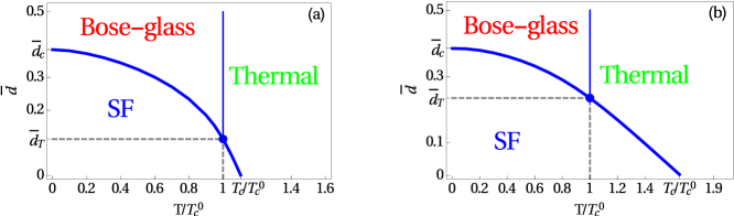
Figure 10: (Color online) Phase diagram in the disorder strength-temperature plane for (a) weakly interacting ${}^{87}{\rm{Rb}}$ gas with $\gamma=0.0007$ and (b) strongly interacting ${}^{4}{\rm{He}}$ gas with $\gamma=0.2366$. Thick and thin lines represent first order and continuous phase transitions, respectively.

Where dimensionless quantities are as follows: $\tilde{n}_{0}(\tilde{r})=n_{0}(r)/\bar{n}$ denotes the condensate density, $\tilde{q}(\tilde{r})=q(r)/\bar{n}$ the Bose-glass order parameter, $\tilde{n}_{{\rm th}}(\tilde{r})=n_{{\rm th}}(r)/\bar{n}$ the thermal density, $\tilde{n}(\tilde{r})=n(r)/\bar{n}$ the total density, $\tilde{r}=r/R_{{\rm{TF}}}$ the s radial coordinate, $\tilde{\mu}=(\mu-d^{2})/\bar{\mu}$ the chemical potential, $\tilde{d}=\frac{\xi}{\mathcal{L}}$ the disorder strength, while $l=\sqrt{\frac{\hbar}{M\varOmega}}$ is the oscillator length, $R_{{\rm{TF}}}=\sqrt{2\bar{\mu}/M\Omega^{2}}$ the TF cloud radius at zero temperature, and $\xi=\frac{l^{2}}{R_{{\rm{TF}}}}$ the coherence length in the center of the trap at zero temperature. The chemical potential in the absence of the disorder at zero temperature $\bar{\mu}=\frac{15^{2/5}}{2}\Big{(}\frac{aN}{l}\Big{)}^{2/5}\hslash\Omega$ is deduced from the normalization condition (5) in the clean case. We also need to write down the dimensionless equivalent of the normalization condition $\eqref{7-1}$:

$$\int_{0}^{\infty}\tilde{n}(\tilde{r})\tilde{r}^{2}d\tilde{r}=\frac{2}{15}.$$ (39)

For the total density $\tilde{n}(\tilde{r})$, the condensate density $\tilde{n}_{0}(\tilde{r})$, the Bose-glass parameter $\tilde{q}(\tilde{r})$, and the thermal density $\tilde{n}_{{\rm th}}(\tilde{r})$ we have three algebraic equations (36)–(38) and one nonlinear partial differential equation (35), which is impossible to solve analytically. Thus we use here again the TF approximation, and neglect the kinetic term in the self-consistency equation (35), which becomes in the superfluid region:

$$\tilde{n}_{0}\left(\tilde{r}\right)=\left[\sqrt{-\tilde{\mu}+2\tilde{n}(\tilde{r})+\tilde{r}^{2}}+\tilde{d}\right]^{2},$$ (40)

where Eqs. (36)–(38) remain the same. Outside the superfluid region Eq. (35) is solved by $\tilde{n}_{0}\left(\tilde{r}\right)=0$.

In the following, we treat first the clean case, where we have no disorder, so as to study only the impact of thermal fluctuations on the BEC system, and then we treat the general case, where disorder and temperature occur simultaneously.

IV.3 Clean case

Even the simpler clean case represents a challenge and has to be treated in the literature either perturbatively with respect to the interaction T-shift1 or fully numerically Stenholm . In the clean case we have no Bose-glass contribution, as we can deduce $\tilde{q}\left(\tilde{r}\right)=0$ from Eq. (36), but only a thermal contribution $\tilde{n}_{{\rm th}}\left(\tilde{r}\right)$ to the total density $\tilde{n}\left(\tilde{r}\right)$. Therefore, in this subsection, two different cases have to be distinguished: in the first one the bosons can be in the condensate or in the excited states, which corresponds to the superfluid region, while in the second one all bosons are in the excited states and there is no condensate any more, so this represents the thermal region.

Using the Robinson approximation Robinson ; Kleinert2 ,

$$\!\!\!\varsigma_{\ \nu}\left(e^{x}\right)=\Gamma\left(1-\nu\right)\left(-x\right)^{\nu-1}+\overset{\infty}{\underset{k=0}{\sum}}\frac{x^{k}}{k!}\varsigma\left(\nu-k\right),\,x<0,\!\!\!$$ (41)

for $\nu=3/2$ the TF-approximated Eqs. (37), (38), and (40) reduce in the superfluid region to:

$$\tilde{n}_{0}\left(\tilde{r}\right) \thickapprox\tilde{\mu}-\tilde{r}^{2}-\frac{2g}{\bar{\mu}}\left(\frac{M}{2\pi\beta\hslash^{2}}\right)^{3/2}\Biggl{[}\Gamma\left(-\frac{1}{2}\right)\sqrt{\beta\bar{\mu}\ \tilde{n}_{0}\left(\tilde{r}\right)}$$

$$+\varsigma\left(\frac{3}{2}\right)-\beta\bar{\mu}\ \tilde{n}_{0}\left(\tilde{r}\right)\varsigma\left(\frac{1}{2}\right)\Biggr{]},$$ (42)

$$\tilde{n}_{{\rm th}}\left(\tilde{r}\right)=\frac{\tilde{\mu}-\tilde{n}_{0}\left(\tilde{r}\right)-\tilde{r}^{2}}{2},$$ (43)

$$\tilde{n}(\tilde{r})=\tilde{n}_{0}\left(\tilde{r}\right)+\tilde{n}_{{\rm th}}\left(\tilde{r}\right).$$ (44)

Equation (42) represents a quadratic equation with respect to $\sqrt{\tilde{n}_{0}\left(\tilde{r}\right)}$ and has, thus, two solutions:

$$\tilde{n}_{0}\left(\tilde{r}\right) =\left[-1+2g\beta\left(\frac{M}{2\pi\beta\hslash^{2}}\right)^{3/2}\varsigma\left(\frac{1}{2}\right)\right]^{-2}$$

$$\!\!\!\!\!\!\!\!\!\!\!\!\!\!\!\left\{-\frac{2g}{\bar{\mu}}\left(\frac{M}{2\pi\beta\hslash^{2}}\right)^{3/2}\sqrt{\pi\beta\bar{\mu}}\right.\pm\Biggl{\{}\frac{4\pi\beta g^{2}}{\bar{\mu}}\left(\frac{M}{2\pi\beta\hslash^{2}}\right)^{3}$$

$$\!\!\!\!\!\!\!\!\!\!\!\!\!\!\!-4\left[\frac{-\tilde{\mu}+\tilde{r}^{2}}{2}+\frac{g}{\bar{\mu}}\left(\frac{M}{2\pi\beta\hslash^{2}}\right)^{3/2}\varsigma\left(\frac{3}{2}\right)\right]$$

$$\!\!\!\!\!\!\!\!\!\!\!\!\!\!\!\left.\times\left[\frac{1}{2}-\beta g\left(\frac{M}{2\pi\beta\hslash^{2}}\right)^{3/2}\varsigma\left(\frac{1}{2}\right)\right]\Biggr{\}}^{\frac{1}{2}}\right\}^{2}.$$ (45)

We choose the one with the positive sign, which corresponds to the numerical solution without Robinson approximation. We insert this solution for the condensate density $\tilde{n}_{0}\left(\tilde{r}\right)$ into Eq. (43) in order to get the thermal density $\tilde{n}_{{\rm th}}\left(\tilde{r}\right)$, and the sum of them then represents the particle density $\tilde{n}(\tilde{r})$ according to Eq. (44). The condensate radius $\tilde{R}_{{\rm TF1}}$, which separates the superfluid from the thermal region, is obtained by setting the derivative of Eq. (42) with respect to $\tilde{n}_{0}\left(\tilde{r}\right)$ to zero, i.e., $\frac{\partial\tilde{r}}{\partial\tilde{n}_{0}\left(\tilde{r}\right)}\Biggl{|}_{\tilde{r}=\tilde{R}_{{\rm TF_{1}}}}=0$. The resulting condensate density $\tilde{n}_{0}\left(\tilde{R}_{{\rm TF1}}\right)$ is inserted again into equation (42) in order to get the following analytical expression for the condensate radius:

$$\tilde{R}_{{\rm TF1}} =\Biggl{[}\tilde{\mu}-\frac{2g}{\bar{\mu}}\left(\frac{M}{2\pi\beta\hslash^{2}}\right)^{3/2}\varsigma\left(\frac{3}{2}\right)$$ (46)

$$+\frac{1}{\bar{\mu}}\left(\frac{M}{2\pi\beta\hslash^{2}}\right)^{3}\frac{4\pi\beta g^{2}}{1-2g\beta\left(\frac{M}{2\pi\beta\hslash^{2}}\right)^{3/2}\varsigma\left(\frac{1}{2}\right)}\Biggr{]}^{\frac{1}{2}}.$$

In the thermal region the condensate vanishes, i.e., $\tilde{n}_{0}(\tilde{r})=0$ and $\tilde{n}_{{\rm th}}\left(\tilde{r}\right)=\tilde{n}(\tilde{r})$. In that case the self-consistency equation (37) reduces to:

$$\tilde{n}\left(\tilde{r}\right)=\frac{g}{\bar{\mu}}\left(\frac{M}{2\pi\beta\hslash^{2}}\right)^{3/2}\varsigma_{\ 3/2}\left(e^{\beta\bar{\mu}\ [\tilde{\mu}-2\tilde{n}\left(\tilde{r}\right)-\tilde{r}^{2}]}\right).$$ (47)

Transcendent Eq. (47) contains the polylogarithmic function $\varsigma_{\ 3/2}$ and, thus, cannot be solved analytically for $\tilde{n}\left(\tilde{r}\right)$. Furthermore, the Robinson formula (41) cannot be applied in the thermal region, since it would yield a diverging density, which is not physical. Thus, the density of the thermal region (47) can be treated only numerically. The cloud radius $\tilde{R}_{{\rm TF2}}$, where the thermal density, and also as a consequence the total density, vanishes is defined here conveniently by the length where the thermal density is equal to $10^{-5}$.

In this subsection we perform our study again for ${}^{87}{\rm{Rb}}$ atoms with the following experimentally realistic parameters: $N=10^{6}$, $\Omega=100{\rm\,{Hz}}$, and $a=5.29\,{\rm{nm}}$. For those parameters the oscillator length is given by $l=2.72{\rm\,{\mu m}}$, the coherence length in the center of the trap turns out to be $\xi=348.89\,{\rm{nm}}$ and the Thomas-Fermi radius reads $R_{{\rm{TF}}}=21.29{\rm\,{\mu m}}$, so the assumption $\xi\ll R_{{\rm{TF}}}$ for the TF approximation is, indeed, fulfilled.

Using those parameter values, we determine the densities of both the superfluid and thermal region. After that the chemical potential $\tilde{\mu}$ has to be fixed using the normalization condition (39), where the total density $\tilde{n}\left(\tilde{r}\right)$ is the combination of the total densities from both the superfluid region and the thermal region. The resulting densities are combined and plotted in Fig. 11 for the temperature $T=60\leavevmode\nobreak\ {\rm nK}$.

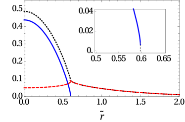
Figure 11: (Color online) Total density $\tilde{n}(\tilde{r})$ (dotted, black), condensate density $\tilde{n}_{0}(\tilde{r})$ (solid, blue), and thermal density $\tilde{n}_{{\rm th}}\left(\tilde{r}\right)$ (dashed, red) with the blow-up of transition region as a function of radial coordinate $\tilde{r}$ for $T=60\leavevmode\nobreak\ {\rm nK}$ yielding $\tilde{\mu}=0.566$.

Figure 11 shows that the condensate density $\tilde{n}_{0}(\tilde{r})$ is maximal at the center of the cloud and decreases when we move away from the center until the condensate radius $\tilde{R}_{{\rm TF1}}$, where it jumps to zero. For the chosen parameters the jump is too small to be visible but it exists as it is shown in the blow-up. The thermal density $\tilde{n}_{{\rm th}}\left(\tilde{r}\right)$ is increasing until reaching its maximum at the condensate radius $\tilde{R}_{{\rm TF1}}$, and then it decreases exponentially to zero. The total density $\tilde{n}(\tilde{r})$ is maximal in the trap center and decreases when one moves away from it, until it vanishes. Note that in the thermal region the total density $\tilde{n}(\tilde{r})$ and the thermal density $\tilde{n}_{{\rm th}}\left(\tilde{r}\right)$ coincide. Although both the condensate density $\tilde{n}_{0}(\tilde{r})$ and the thermal density $\tilde{n}_{{\rm th}}\left(\tilde{r}\right)$ are discontinuous at the condensate radius $\tilde{R}_{{\rm TF1}}$, the total density $\tilde{n}\left(\tilde{r}\right)$ remains continuous but reveals a discontinuity of the first derivative. We conclude from Fig. 11 that the condensate is situated in the trap center, while the bosons in the excited states are located at the border of the trap.

In order to study how the temperature changes the respective Thomas-Fermi radii, we plot them in Fig. 12a as functions of the temperature $T$. This figure reveals the existence of two phases: a superfluid phase, where the bosons are either in the condensate or in the excited

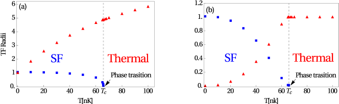
Figure 12: (Color online) (a) Condensate radius $\tilde{R}_{{\rm TF1}}$ (square, blue) and cloud radius $\tilde{R}_{{\rm TF2}}$ (triangle, red) and (b) fractional number of condensed particles $N_{0}/N$ (square, blue) and in the excited states $N_{{\rm{th}}}/N$ (triangle, red) as a function of temperature $T$.

states, and a thermal phase, where all particles are in the excited states. The condensate radius $\tilde{R}_{{\rm TF1}}$ decreases with the temperature until it vanishes at the critical temperature $T_{{\rm{c}}}$ marking the location of the phase transition. The critical temperature $T_{{\rm{c}}}$ is the solution of the equality $\tilde{R}_{{\rm TF1}}=0$, i.e., we get from Eq. (46)

$$\frac{4\pi g^{2}T_{{\rm{c}}}^{2}}{\bar{\mu}k_{B}}\left(\frac{Mk_{B}}{2\pi\hslash^{2}}\right)^{3} +\left[\tilde{\mu}_{c}-\frac{2g}{\bar{\mu}}\left(\frac{Mk_{B}T_{{\rm{c}}}}{2\pi\hslash^{2}}\right)^{3/2}\varsigma\left(\frac{3}{2}\right)\right]$$

$$\!\!\!\!\!\!\!\!\!\!\!\!\!\!\!\!\!\!\!\!\!\!\!\!\!\!\!\!\!\!\!\!\!\!\!\!\!\!\!\!\!\!\!\!\!\times\left[1-\frac{2g\sqrt{T_{{\rm{c}}}}}{k_{B}}\left(\frac{Mk_{B}}{2\pi\hslash^{2}}\right)^{3/2}\varsigma\left(\frac{1}{2}\right)\right]=0,$$ (48)

where $\tilde{\mu}_{c}$ is the critical chemical potential at the phase transition, whose first-order correction follows from Eq. (47)

$$\tilde{\mu}_{c}=2\tilde{n}(0)=\frac{2g}{\bar{\mu}}\left(\frac{Mk_{B}T_{{\rm{c}}}}{2\pi\hslash^{2}}\right)^{3/2}\varsigma\left(\frac{3}{2}\right).$$ (49)

For the chosen parameters we obtain by solving the system (48) and (49) the values $T_{{\rm{c}}}=65.71\leavevmode\nobreak\ {\rm nK}$ and $\tilde{\mu}_{c}=0.08$, the former agreeing well with Fig. 12a. The critical temperature can be compared with the one given via the first-order correction T-shift1 ; T-shift-2

$$\frac{T_{{\rm{c}}}-T_{{\rm{c}}}^{0}}{T_{{\rm{c}}}^{0}}=-1.33\frac{a}{l}N^{1/6},$$ (50)

where $T_{{\rm{c}}}^{0}=\frac{\hbar\Omega}{k_{B}}\left(\frac{N}{\varsigma\left(3\right)}\right)^{1/3}$ denotes the critical temperature for the non-interacting BEC. Equation (50) is obtained by inserting Eqs. (47) and (49) into the normalization condition (39) and by expanding the result to first order with respect to the contact interaction strength $g$. We read off from Eq. (50) that the repulsive interaction reduces the critical temperature. For the chosen parameters the critical temperature of the ideal Bose gas reads $T_{{\rm{c}}}^{0}=71.87\leavevmode\nobreak\ {\rm nK}$. According to formula (50) the critical temperature for the interacting case has the value $T_{{\rm{c}}}=70.01\leavevmode\nobreak\ {\rm nK}$, which is nearly the one obtained above and in Fig. 12a. On the other hand, the cloud radius $\tilde{R}_{{\rm TF2}}$ turns out to increase with the temperature.

In Fig. 12b the fractional number of the condensate $N_{0}/N=\frac{15}{2}\int_{0}^{\tilde{R}_{{\rm{TF1}}}}\tilde{r}^{2}\tilde{n}_{0}\left(\tilde{r}\right)d\tilde{r}$ is plotted as a function of the temperature $T$. We note that $N_{0}/N$ is equal to one at zero temperature, i.e., all particles are in the condensate, then it decreases with the temperature until it vanishes at $T_{{\rm{c}}}$, marking the end of the superfluid phase and the beginning of the thermal phase. Conversely, the fractional number of the particles in the thermal states $N_{{\rm{th}}}/N=\frac{15}{2}\int_{0}^{\tilde{R}_{{\rm{TF2}}}}\tilde{r}^{2}\tilde{n}_{{\rm th}}\left(\tilde{r}\right)d\tilde{r}$, where $N_{{\rm{th}}}$ is the number of particles in the excited states, increases with the temperature until being maximal at $T_{{\rm{c}}}$, and then it remains constant and equals to one in the thermal phase since all particles are in the excited states.

In order to study for which temperature range the TF approximation is valid, we plot the ratio of the condensate density at the condensate radius $\tilde{n}_{0}(\tilde{R}_{{\rm TF1}})$ with respect to the condensate density at the center of the BEC $\tilde{n}_{0}(0)$ as a function of the temperature in Fig. 13. We read off that this ratio is negligible for $T<T_{{\rm{c}}}$ and has a sudden jump for $T\approx T_{{\rm{c}}}$. This means that the TF approximation is valid in the superfluid phase but not in the transition region, where one would have to go beyond the TF approximation and take the influence of the kinetic energy in Eq. (35) into account.

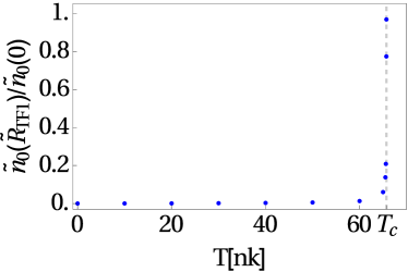
Figure 13: (Color online) Ratio of $\tilde{n}_{0}(\tilde{R}_{{\rm TF1}})$ and $\tilde{n}_{0}(0)$ as a function of temperature $T$.

IV.4 Disordered case

In this subsection we consider the BEC system to be in a disordered landscape as well as at finite temperature. Thus, we investigate now the effect of both temperature and disorder on the properties of the system, in particular on the respective densities and Thomas-Fermi radii. Generically, we have to distinguish three different regions as illustrated in Fig. 14: the superfluid region, where the bosons are distributed in the condensate as well as in the minima of the disorder potential and in the excited states, the Bose-glass region, where there are no bosons in the condensate so that all bosons contribute to the local Bose-Einstein condensates or to the excited states, and the thermal region, where all bosons are in the excited states. In the following we analyze the properties of each region separately. To this end, we have to solve the dimensionless algebraic Eqs. (36)–(38), (40) and the normalization condition (39). We start first with the thermal region and the Bose-glass region, since they are easier to treat, and then we focus on the superfluid region.

IV.4.1 Thermal region

In the thermal region only the thermal component contributes to the total density, so we have $\tilde{n}_{0}(\tilde{r})=\tilde{q}\left(\tilde{r}\right)=0$ and $\tilde{n}_{{\rm th}}\left(\tilde{r}\right)=\tilde{n}(\tilde{r})$. In this case we just need Eq. (37), which reduces to

$$\tilde{n}_{{\rm th}}\left(\tilde{r}\right)=\frac{g}{\bar{\mu}}\left(\frac{M}{2\pi\beta\hslash^{2}}\right)^{3/2}\varsigma_{\ 3/2}\left(e^{\beta\bar{\mu}\ [\tilde{\mu}-2\tilde{n}_{{\rm th}}\left(\tilde{r}\right)-\tilde{r}^{2}]}\right),$$ (51)

and can only be solved numerically. The cloud radius $\tilde{R}_{{\rm TF3}}$, which characterizes the end of the thermal region, is determined here by setting $\tilde{n}_{{\rm th}}\left(\tilde{R}_{{\rm TF3}}\right)=10^{-5}$.

IV.4.2 Bose-Glass region

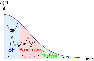
Figure 14: (Color online) Illustration for the distribution of bosons in the superfluid (SF) region, where the condensate density $\tilde{n}_{0}(\tilde{r})$, the Bose-glass order parameter $\tilde{q}\left(\tilde{r}\right),$ and the thermal density $\tilde{n}_{{\rm th}}\left(\tilde{r}\right)$ contribute to the total density $\tilde{n}(\tilde{r})=\tilde{n}_{0}(\tilde{r})+\tilde{q}\left(\tilde{r}\right)+\tilde{n}_{{\rm th}}\left(\tilde{r}\right)$. In the Bose-glass region the condensate vanishes and in the thermal region all particles are in the excited states.

In the Bose-glass region the condensate vanishes, i.e., $\tilde{n}_{0}(\tilde{r})=0$, and we only need the self-consistency equations (36)–(38), which reduce to:

$$\tilde{q}\left(\tilde{r}\right)=\frac{\tilde{\mu}-\tilde{r}^{2}}{2}-\frac{g}{\bar{\mu}}\left(\frac{M}{2\pi\beta\hslash^{2}}\right)^{3/2}\varsigma\left(\frac{3}{2}\right),$$ (52)

$$\tilde{n}_{{\rm th}}\left(\tilde{r}\right)=\frac{g}{\bar{\mu}}\left(\frac{M}{2\pi\beta\hslash^{2}}\right)^{3/2}\varsigma\left(\frac{3}{2}\right),$$ (53)

$$\tilde{n}(\tilde{r})=\frac{\tilde{\mu}-\tilde{r}^{2}}{2}.$$ (54)

Note that Eq. (53) reveals that the thermal density in the Bose-glass region remains constant, which we consider to be an artifact of the TF approximation. The Bose-glass radius $\tilde{R}_{{\rm TF2}}$, which characterizes the end of the Bose-glass region and the beginning of the thermal region, is determined by setting $\tilde{q}\left(\tilde{R}_{{\rm TF_{2}}}\right)=0$ in Eq. (52), so we get $\tilde{R}_{{\rm TF2}}=\sqrt{\tilde{\mu}-2\frac{g}{\bar{\mu}}\left(\frac{M}{2\pi\beta\hslash^{2}}\right)^{3/2}\varsigma\left(\frac{3}{2}\right)}$.

IV.4.3 Superfluid region

In the superfluid region all densities contribute to the total density and the four algebraic coupled equations (36)–(38) and (40) have to be taken into account. We solve them according to the following strategy. At first we get from Eqs. (36)–(38) one self-consistency equation for the condensate density $\tilde{n}_{0}(\tilde{r})$:

$$\left[\sqrt{\tilde{n}_{0}(\tilde{r})}-\tilde{d}\right]^{2}+\tilde{\mu}-\tilde{r}^{2}-\frac{2\tilde{n}_{0}^{3/2}(\tilde{r})}{\sqrt{\tilde{n}_{0}(\tilde{r})}-\tilde{d}}$$

$$-\frac{2g}{\bar{\mu}}\left(\frac{M}{2\pi\beta\hslash^{2}}\right)^{3/2}\varsigma_{\ 3/2}\left(e^{-\beta\bar{\mu}\ \left[\sqrt{\tilde{n}_{0}(\tilde{r})}-\tilde{d}\right]^{2}}\right) =0.$$ (55)

In the superfluid region we can apply the Robinson formula (41) for $\nu=3/2$ to approximate Eq. (55) as

$$0= \left[\sqrt{\tilde{n}_{0}(\tilde{r})}-\tilde{d}\right]^{3}\left[1-2g\beta\left(\frac{M}{2\pi\beta\hslash^{2}}\right)^{3/2}\varsigma\left(\frac{1}{2}\right)\right]$$

$$+2\left[g\left(\frac{M}{2\pi\beta\hslash^{2}}\right)^{3/2}\Gamma\left(-\frac{1}{2}\right)\sqrt{\beta/\bar{\mu}}+3\tilde{d}\right]$$

$$\times\left[\sqrt{\tilde{n}_{0}(\tilde{r})}-\tilde{d}\right]^{2}+2\tilde{d}^{3}+\left[\sqrt{\tilde{n}_{0}(\tilde{r})}-\tilde{d}\right]$$

$$\times\left[2\frac{g}{\bar{\mu}}\left(\frac{M}{2\pi\beta\hslash^{2}}\right)^{3/2}\varsigma\left(\frac{3}{2}\right)+6\tilde{d}^{2}-\tilde{\mu}+\tilde{r}^{2}\right],$$ (56)

After having solved Eq. (56), we insert the result into the other algebraic equations. To this end we have to rewrite the other densities as functions of the condensate density $\tilde{n}_{0}(\tilde{r})$. From Eqs. (36) and (40) we get

$$\tilde{q}\left(\tilde{r}\right)=\frac{\tilde{d}\tilde{n}_{0}\left(\tilde{r}\right)}{\sqrt{\tilde{n}_{0}(\tilde{r})}-\tilde{d}},$$ (57)

and from Eqs. (37) and (40) after applying the Robinson formula (41) for $\nu=3/2$, we obtain:

$$\tilde{n}_{{\rm th}}\left(\tilde{r}\right) =\frac{g}{\bar{\mu}}\left(\frac{M}{2\pi\beta\hslash^{2}}\right)^{3/2}\Biggl{[}\Gamma\left(-\frac{1}{2}\right)\sqrt{\beta\bar{\mu}}\left[\sqrt{\tilde{n}_{0}(\tilde{r})}-\tilde{d}\right]$$

$$+\varsigma\left(\frac{3}{2}\right)-\beta\bar{\mu}\ \left[\sqrt{\tilde{n}_{0}(\tilde{r})}-\tilde{d}\right]^{2}\varsigma\left(\frac{1}{2}\right)\Biggr{]}.$$ (58)

Thus, we have to solve the cubic self-consistency equation for the condensate density (56) via the Cardan method and insert the solution into Eqs. (57), (58), and (38) in order to get directly $\tilde{q}\left(\tilde{r}\right)$, $\tilde{n}_{{\rm th}}\left(\tilde{r}\right)$, and $\tilde{n}(\tilde{r})$, respectively. The cubic Eq. (56) has only one physical solution. To determine the border of the superfluid region, i.e., the condensate radius $\tilde{R}_{{\rm{TF1}}}$, where the solution of Eq. (56) vanishes and which characterizes the edge of the superfluid region as well as the beginning of the Bose-glass region, we determine the first derivative of Eq. (56) with respect to $\tilde{n}_{0}\left(\tilde{r}\right)$, and then we set $\frac{\partial\tilde{r}}{\partial\tilde{n}_{0}\left(\tilde{r}\right)}\Biggl{|}_{\tilde{r}=\tilde{R}_{{\rm TF_{1}}}}=0$, which yields:

$$3 \left[\sqrt{\tilde{n}_{0}\left(\tilde{R}_{{\rm TF1}}\right)}-\tilde{d}\right]^{2}\left[1-2g\beta\left(\frac{M}{2\pi\beta\hslash^{2}}\right)^{3/2}\varsigma\left(\frac{1}{2}\right)\right]$$

$$+4\left[g\left(\frac{M}{2\pi\beta\hslash^{2}}\right)^{3/2}\Gamma\left(-\frac{1}{2}\right)\sqrt{\beta/\bar{\mu}}+3\tilde{d}\right]$$

$$\times\left[\sqrt{\tilde{n}_{0}\left(\tilde{R}_{{\rm TF1}}\right)}-\tilde{d}\right]+\Biggl{[}2\frac{g}{\bar{\mu}}\left(\frac{M}{2\pi\beta\hslash^{2}}\right)^{3/2}\varsigma\left(\frac{3}{2}\right)$$

$$+6\tilde{d}^{2}-\tilde{\mu}+\tilde{R}_{{\rm TF1}}^{2}\Biggr{]}=0.$$ (59)

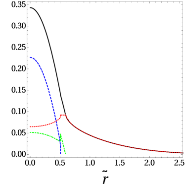
Figure 15: (Color online) Spatial distribution of total density $\tilde{n}(\tilde{r})$ (solid, black), condensate density $\tilde{n}_{0}(\tilde{r})$ (dashed, blue), Bose-glass order parameter $\tilde{q}(\tilde{r})$ (dotted-dashed, green), and thermal density $\tilde{n}_{{\rm th}}\left(\tilde{r}\right)$ (dotted, red) as functions of the radial coordinate $\tilde{r}$ for $\tilde{d}=0.088$. Since $N$ is fixed, $\tilde{\mu}$ can be determined and results in $\tilde{\mu}=0.535$.

This result we insert back into Eq. (56) in order to get the analytical expression of the condensate radius $\tilde{R}_{{\rm TF1}}$. As the result is too involved, it is not explicitly displayed here.

IV.5 Thomas-Fermi densities

Now we perform our study for ${}^{87}{\rm{Rb}}$ atoms and the same experimentally realistic parameters as in Subsection IV.C and choose the temperature to be $T=60\leavevmode\nobreak\ {\rm nK}.$ To this end, we first calculate the densities in the thermal region, the Bose-glass region, and the superfluid region. After that we fix the chemical potential $\tilde{\mu}$ using the normalization condition (39), where the total density $\tilde{n}(\tilde{r})$ is the sum of the densities from all regions. The resulting densities are plotted in Fig. 15.

Figure 15 shows that the condensate density $\tilde{n}_{0}(\tilde{r})$ is maximal at the center of the cloud, then it decreases until reaching its minimum at the condensate radius $\tilde{R}_{{\rm TF1}}=0.506$. The Bose-glass order parameter $\tilde{q}(\tilde{r})$ is also maximal at the center of the cloud, decreases until the condensate radius $\tilde{R}_{{\rm TF1}}$ where it jumps upward, then decreases until reaching its minimum at the Bose-glass radius $\tilde{R}_{{\rm TF2}}=0.588$. The thermal density $\tilde{n}_{{\rm th}}\left(\tilde{r}\right)$ is behaving differently: it increases until reaching its maximum at the condensate radius $\tilde{R}_{{\rm TF1}}$, it stays constant until the Bose-glass radius $\tilde{R}_{{\rm TF2}}$, then it decreases exponentially to zero. Note that in the thermal region the thermal

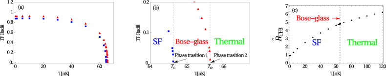
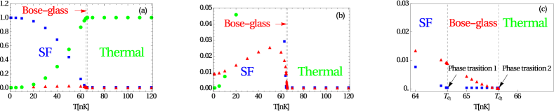
Figure 16: (Color online) (a) Condensate radius $\tilde{R}_{{\rm TF1}}$ (square, blue) and Bose-glass radius $\tilde{R}_{{\rm TF2}}$ (triangle, red) and (b) blow-up of Bose-glass region (c) cloud radius $\tilde{R}_{{\rm TF3}}$ (dotted, black) as functions of temperature $T$.

Figure 17: (Color online) (a) Fractional number of condensed particles $N_{0}/N$ (square, blue), in disconnected local minicondensates $Q/N$ (triangle, red), and in excited states $N_{{\rm{th}}}/N$ (dotted, green) , (b) blow-up of disconnected local minicondensates $Q/N$, and (c) blow-up of Bose-glass phase as functions of temperature $T$.

density coincides with the total density. The fact that the thermal density remains constant in the Bose-glass region is considered to be an artifact of the TF approximation. The total density $\tilde{n}(\tilde{r})$ is maximal in the center of the trap and decreases when we move away from the center until it vanishes at the cloud radius $\tilde{R}_{{\rm TF3}}=4.642$. We note also that, at the condensate radius $\tilde{R}_{{\rm TF1}}$, a downward jump of the condensate density $\tilde{n}_{0}(\tilde{r})$, an upward jump of the Bose-glass order parameter $\tilde{q}(\tilde{r})$, and an upward jump of the thermal density $\tilde{n}_{{\rm th}}\left(\tilde{r}\right)$ occur in such a way that the total density $\tilde{n}(\tilde{r})$ remains continuous but reveals a discontinuity of the first derivative. The TF approximation captures the properties of the system within the superfluid region, the Bose-glass region and the thermal region but not at the transition point between two regions, namely, between the superfluid region and the Bose-glass region as well as between the Bose-glass region and the thermal region. This represents another artifact of the applied TF approximation.

In the following we investigate separately the impact of increasing the temperature $T$ and the disorder strength $\tilde{d}$ on the properties of the dirty boson system, namely, the Thomas-Fermi radii and the fractional number of condensed particles $N_{0}/N$, in the disconnected local minicondensates $Q/N$, and in the excited states $N_{{\rm{th}}}/N$.

IV.6 Effects of the temperature

We start by studying the influence of the temperature on the dirty boson system. To this end, we fix the disorder strength at $\tilde{d}=0.088$ and increase the temperature $T$. The Thomas-Fermi radii are plotted as functions of the temperature $T$ in Fig. 17. Figure  17a shows that both the condensate radius $\tilde{R}_{{\rm{TF1}}}$ and the Bose-glass radius $\tilde{R}_{{\rm{TF2}}}$ decrease with the temperature $T$ until they vanish. The blow-up in Fig. 17b reveals that the condensate radius $\tilde{R}_{{\rm{TF1}}}$ vanishes at $T_{{\rm{\rm{c1}}}}=64.625\leavevmode\nobreak\ {\rm nK}$, which corresponds to a phase transition from the superfluid to the Bose-glass. This critical value of the temperature is obtained by setting the condensate radius $\tilde{R}_{{\rm TF1}}$ to zero. Thus, superfluidity is destroyed in our model at a critical temperature, where approximately our TF approximation breaks down. The Bose-glass radius $\tilde{R}_{{\rm{TF2}}}$ vanishes at $T_{{\rm{\rm{c2}}}}=65.625\leavevmode\nobreak\ {\rm nK}$, which corresponds to a phase transition from the Bose-glass to the thermal. This critical value of the temperature is obtained by setting the Bose-glass radius $\tilde{R}_{{\rm TF2}}$ to zero. The existence of those two phase transitions means that we are qualitatively above the triple point introduced for the homogeneous case in Fig. 10. Note that the difference of both critical temperatures $\triangle T_{{\rm{\rm{c}}}}=T_{{\rm{\rm{c2}}}}-T_{{\rm{\rm{c1}}}}$ is quite small, which is expected, since one can deduce from Eq. (51) that the shift $\triangle T$ goes quadratically with the disorder strength $\tilde{d}$, which means that the linear temperature shift vanishes in agreement with the finding of Ref. Timmer . Contrary to that, the cloud radius $\tilde{R}_{{\rm TF3}}$ increases monotonously with the temperature $T$ in Fig 17c.

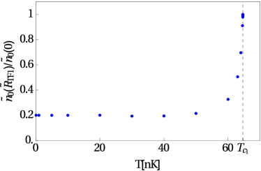
Figure 18: (Color online) Ratio $\tilde{n}_{0}(\tilde{R}_{{\rm TF1}})/\tilde{n}_{0}(0)$ as a function of temperature $T$.

The occupancy fraction of the condensate $N_{0}/N=\frac{15}{2}\int_{0}^{\tilde{R}_{{\rm{TF1}}}}\tilde{r}^{2}\tilde{n}_{0}\left(\tilde{r}\right)d\tilde{r}$, of the disconnected minicondensates $Q/N=\frac{15}{2}\int_{0}^{\tilde{R}_{{\rm{TF2}}}}\tilde{r}^{2}\tilde{q}\left(\tilde{r}\right)d\tilde{r}$, and of the excited states $N_{{\rm{th}}}/N=\frac{15}{2}\int_{0}^{\tilde{R}_{{\rm{TF3}}}}\tilde{r}^{2}\tilde{n}_{{\rm th}}\left(\tilde{r}\right)d\tilde{r}$ are plotted in Fig. 17a as functions of the temperature $T$. We remark that in the superfluid phase $N_{0}/N$ decreases with the temperature $T$ until vanishing at $T_{{\rm{\rm{c_{1}}}}}$ marking the end of the superfluid phase and the beginning of the Bose-glass phase as it is illustrated in the blow-up in Fig 17c. Conversely, in Fig 17b we see that $Q/N$ increases with the temperature $T$ until reaching maximum at about $T=50\leavevmode\nobreak\ {\rm nK}$, then decreases until vanishing at $T_{{\rm{\rm{c2}}}}$ marking the end of the Bose-glass phase and the beginning of the thermal phase as shown in the blow-up in Fig 17c. In Fig. 17a $N_{{\rm{th}}}/N$ increases starting from zero with the temperature $T$ until being equal to one at $T_{{\rm{\rm{c_{2}}}}}$, then it remains constant. We conclude that, by increasing the temperature until $T=50\leavevmode\nobreak\ {\rm nK}$, more and more particles are leaving the condensate towards the local minicondensates or the excited states. For the temperature values $50\leavevmode\nobreak\ {\rm nK}<T<T_{{\rm{\rm{c_{1}}}}}$ the particles are leaving both the condensate and the local minicondensates towards the excited states. When the condensate vanishes at the critical temperature $T_{{\rm{\rm{c_{1}}}}}$, the particles keep leaving the local minicondensates towards the excited states until the critical temperature $T_{{\rm{\rm{c_{2}}}}}$, where all particles are in the excited states.

In order to study for which temperature range the TF approximation is valid, we plot the ratio of the jump of the condensate density at the Thomas-Fermi condensate radius $\tilde{n}_{0}(\tilde{R}_{{\rm TF_{1}}})$ with respect to the condensate density at the center of the BEC $\tilde{n}_{0}(0)$ as a function of the temperature $T$ in Fig. 18. We note that this ratio is negligible for $T<T_{{\rm{c_{1}}}}$ and has a sudden jump for $T\approx T_{{\rm{c}}}$. This means that the TF approximation is valid in the superfluid phase but not in the transition region from the superfluid to the Bose-glass, where one would have to go beyond the TF approximation and take the effect of the kinetic energy in Eq. (35) into account.

IV.7 Disorder effects

Now we study the influence of the disorder on the dirty boson system. To this end, we choose the temperature to be $T=60\leavevmode\nobreak\ {\rm nK}$ and consider an increase of the disorder strength $\tilde{d}$.

In order to determine for which range of the disorder strength $\tilde{d}$ the TF approximation is valid, we plot the ratio of the condensate density at the Thomas-Fermi condensate radius $\tilde{n}_{0}(\tilde{R}_{{\rm TF_{1}}})$ with respect to the condensate density at the center of the BEC $\tilde{n}_{0}(0)$ as a function of the disorder strength $\tilde{d}$ in Fig. 19. As only a moderate density jump of about 50% should be reasonable, our approach is restricted to a dimensionless disorder strength of about $\tilde{d}\simeq 0.11$. For a larger disorder strength $\tilde{d}$ one would have to go beyond the TF approximation and take the influence of the kinetic energy in (35) into account.

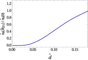
Figure 19: (Color online) Ratio $\tilde{n}_{0}(\tilde{R}_{{\rm TF1}})/\tilde{n}_{0}(0)$ as a function of disorder strength $\tilde{d}$.

The Thomas-Fermi radii are plotted as functions of the disorder strength $\tilde{d}$ in Fig. 20. According to the behavior of the Thomas-Fermi radii, we distinguish between two different disorder regimes: the weak disorder regime and the intermediate one. Figure  20a shows that, when the disorder strength $\tilde{d}$ increases, the condensate radius $\tilde{R}_{{\rm{TF1}}}$ increases slightly, then decreases until zero, which corresponds to a phase transition at about $\tilde{d}_{{\rm{\rm{c}}}}=0.181$. This critical value of the disorder strength is obtained by setting the cloud radius $\tilde{R}_{{\rm TF1}}$ to zero. Thus, superfluidity is destroyed in our model at a critical disorder strength, where approximately our TF approximation breaks down. Contrarily, the Bose-glass radius $\tilde{R}_{{\rm{TF2}}}$ decreases when the disorder strength $\tilde{d}$ increases in the weak disorder regime, then increases in the intermediate disorder regime until the phase transition, then it becomes constant, so that the bosonic cloud has a maximal Bose-glass radius of $\underset{\tilde{d}\rightarrow\infty}{{\rm lim}}$ $\tilde{R}_{{\rm TF2}}=0.647$. Figure 20a

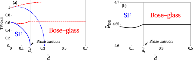
Figure 20: (Color online) (a) Condensate radius $\tilde{R}_{{\rm TF1}}$ at $T=60\leavevmode\nobreak\ {\rm nK}$ (solid, blue) and at $T=0$ (dotted, blue), Bose-glass radius $\tilde{R}_{{\rm TF2}}$ at $T=60\leavevmode\nobreak\ {\rm nK}$ (dashed, red) and at $T=0$ (dotted-dashed, red) and (b) cloud radius $\tilde{R}_{{\rm TF3}}$ at $T=60\leavevmode\nobreak\ {\rm nK}$ (solid, black) as functions of disorder strength $\tilde{d}$.

shows also that in the weak disorder regime the condensate radius $\tilde{R}_{{\rm{TF1}}}$ and the Bose-glass radius $\tilde{R}_{{\rm{TF2}}}$ coincide, i.e., there is no Bose-glass region, only the superfluid and the thermal regions exist. Furthermore, comparing the condensate radius $\tilde{R}_{{\rm{TF1}}}$ and the Bose-glass radius $\tilde{R}_{{\rm{TF2}}}$ at finite temperature with the corresponding ones at zero temperature reveals that increasing the temperature decreases the critical disorder strength value $\tilde{d}_{{\rm{\rm{c}}}}$, where the phase transition is taking place. In Fig 20b the cloud radius $\tilde{R}_{{\rm TF3}}$ decreases with the disorder strength $\tilde{d}$ in the weak disorder regime, then increases with it in the intermediate disorder regime until becoming constant at the phase transition, so that the bosonic cloud has a maximal size of $\underset{\tilde{d}\rightarrow\infty}{{\rm lim}}$ $\tilde{R}_{{\rm TF3}}=4.649$.

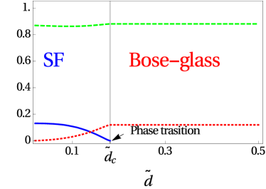
Figure 21: (Color online) Fractional number of condensed particles $N_{0}/N$ (solid, blue), in disconnected local minicondensates $Q/N$ (dotted, red), and in excited states $N_{{\rm{th}}}/N$ (dashed, green), as functions of disorder strength $\tilde{d}$.

In Fig. 21 the fractional number of the condensate $N_{0}/N$, in the disconnected minicondensates $Q/N$, and in the excited states $N_{{\rm{th}}}/N$ are plotted as functions of the disorder strength $\tilde{d}$. We remark that in the superfluid phase $N_{0}/N$ decreases with the disorder strength $\tilde{d}$ until vanishing at $\tilde{d}_{{\rm{\rm{c}}}},$ marking the end of the superfluid phase and the beginning of the Bose-glass phase. Conversely, $Q/N$ and $N_{{\rm{th}}}/N$ increase with the disorder strength $\tilde{d}$, i.e., more and more particles are leaving the condensate towards the local minicondensates or the excited states. In the Bose-glass phase, both fractions $Q/N$ and $N_{{\rm{th}}}/N$ remain constant.

V Conclusions

From the presented results we see that for an isotropically trapped dirty Bose gas the TF approximation provides better description in three dimensions than in one dimension Paper1 due to the fact that the fluctuations are more pronounced in lower dimensions. Additionally, at zero temperature the respective densities and the Thomas-Fermi radii obtained via the TF approximation and the variational method turn out to agree qualitatively well. In particular, a first-order quantum phase transition from the superfluid phase to the Bose-glass phase is detected at a critical disorder strength, whose value is of the same order as the one determined in Refs. Nattermann ; Natterman2 .

At finite temperature three regions coexist, namely, the superfluid region, the Bose-glass region, and the thermal region. Depending on the parameters of the system, three phase transitions were detected, namely, from the superfluid to the Bose-glass phase, from the Bose-glass to the thermal phase, and from the superfluid to the thermal phase. We have also studied in detail the properties of phase transitions. The obtained results could be particularly useful for a quantitative analysis of on going experiments with dirty bosons in three-dimensional harmonic traps.

- (1) M. P. A. Fisher, P. B. Weichman, G. Grinstein, and D. S. Fisher, Phys. Rev. B 40, 546 (1989).
- (2) B. C. Crooker, B. Hebral, E. N. Smith, Y. Takano, and J. D. Reppy, Phys. Rev. Lett. 51, 666 (1983).
- (3) M. H. W. Chan, K. I. Blum, S. Q. Murphy, G. K. S. Wong, and J. D. Reppy, Phys. Rev. Lett. 61, 1950 (1988).
- (4) G. K. S. Wong, P. A. Crowell, H. A. Cho, and J. D. Reppy, Phys. Rev. Lett. 65, 2410 (1990).
- (5) J.D. Reppy, J. Low Temp. Phys. 87, 205 (1992).
- (6) R. Folman, P. Krüger, J. Schmiedmayer, J. Denschlag, and C. Henkel, Adv. At. Mol. Opt. Phys. 48, 263 (2002).
- (7) D. W. Wang, M. D. Lukin, and E. Demler, Phys. Rev. Lett. 92, 076802 (2004).
- (8) T. Schumm, J. Esteve, C. Figl, J. B. Trebbia, C. Aussibal, H. Nguyen, D. Mailly, I. Bouchoule, C. I. Westbrook, and A. Aspect, Eur. Phys. J. D 32, 171 (2005).
- (9) J. Fortágh and C. Zimmermann, Rev. Mod. Phys. 79, 235 (2007).
- (10) P. Krüger, L. M. Andersson, S. Wildermuth, S. Hofferberth, E. Haller, S. Aigner, S. Groth, I. Bar-Joseph, and J. Schmiedmayer, Phys. Rev. A 76, 063621 (2007).
- (11) J. C. Dainty (Ed.), Laser Speckle and Related Phenomena, Springer, Berlin, 1975.
- (12) J. E. Lye, L. Fallani, M. Modugno, D. S.Wiersma, C. Fort, and M. Inguscio, Phys. Rev. Lett. 95, 070401 (2005).
- (13) D. Clément, A. F. Varón, M. Hugbart, J. A. Retter, P. Bouyer, L. Sanchez-Palencia, D. M. Gangardt, G. V. Shlyapnikov, and A. Aspect, Phys. Rev. Lett. 95, 170409 (2005).
- (14) J. Billy, V. Josse, Z. Zuo, A. Bernard, B. Hambrecht, P. Lugan, D. Clément, L. Sanchez-Palencia, P. Bouyer, and A. Aspect, Nature (London) 453, 891 (2008).
- (15) J. W. Goodman, Speckle Phenomena in Optics: Theory and Applications, Viva Books Private Limited, First Edition, 2010.
- (16) U. Gavish and Y. Castin, Phys. Rev. Lett. 95, 020401 (2005).
- (17) B. Gadway, D. Pertot, J. Reeves, M. Vogt, and D. Schneble, Phys. Rev. Lett. 107, 145306 (2011).
- (18) B. Damski, J. Zakrzewski, L. Santos, P. Zoller, and M. Lewenstein, Phys. Rev. Lett. 91, 080403 (2003).
- (19) T. Schulte, S. Drenkelforth, J. Kruse, W. Ertmer, J. Arlt, K. Sacha, J. Zakrzewski, and M. Lewenstein, Phys. Rev. Lett. 95, 170411 (2005).
- (20) G. Roati, C. D’Errico, L. Fallani, M. Fattori, C. Fort, M. Zaccanti, G. Modugno, M. Modugno, and M. Inguscio, Nature (London) 453, 895 (2008).
- (21) A. L. Gaunt, T. F. Schmidutz, I. Gotlibovych, R. P. Smith, and Z. Hadzibabic, Phys. Rev. Lett. 110, 200406 (2013).
- (22) N. N. Bogoliubov, J. Phys. (USSR) 11, 23 (1947).
- (23) K. Huang and H. F. Meng, Phys. Rev. Lett. 69, 644 (1992).
- (24) S. Giorgini, L. Pitaevskii, and S. Stringari, Phys. Rev. B 49, 12938 (1994).
- (25) M. Kobayashi and M. Tsubota, Phys. Rev. B 66, 174516 (2002).
- (26) B. Abdullaev and A. Pelster, Europ. Phys. J. D 66, 314 (2012).
- (27) A. Boudjemaa, Phys. Rev. A 91, 053619 (2015).
- (28) A. V. Lopatin and V. M. Vinokur, Phys. Rev. Lett. 88, 235503 (2002).
- (29) G. M. Falco, A. Pelster, and R. Graham, Phys. Rev. A 75, 063619 (2007).
- (30) R. Graham and A. Pelster, Int. J. Bif. Chaos 19, 2745 (2009).
- (31) C. Krumnow and A. Pelster, Phys. Rev. A 84, 021608(R) (2011).
- (32) B. Nikoli, A. Balaž, and A. Pelster, Phys. Rev. A 88, 013624 (2013).
- (33) M. Ghabour and A. Pelster, Phys. Rev. A 90, 063636 (2014).
- (34) A. Boudjemaa, Phys. Lett. A 379, 2484 (2015).
- (35) A. Boudjemaa, J. Low Temp. Phys. 180, 377 (2015).
- (36) P. Navez, A. Pelster, and R. Graham, App. Phys. B 86, 395 (2007).
- (37) V. I. Yukalov and R. Graham, Phys. Rev. A 75, 023619 (2007).
- (38) G.E. Astrakharchik, J. Boronat, J. Casulleras, and S. Giorgini, Phys. Rev. A 66, 023603 (2002).
- (39) H. Meier and M. Wallin, Phys. Rev. Lett. 108, 055701 (2012).
- (40) R. Ng and E. S. Sørensen, Phys. Rev. Lett. 114, 255701 (2015).
- (41) G. M. Falco, A. Pelster, and R. Graham, Phys. Rev. A 76, 013624 (2007).
- (42) B. Shapiro, Phys. Rev. Lett. 99, 060602 (2007).
- (43) T. Nattermann and V. L. Pokrovsky, Phys. Rev. Lett. 100, 060402 (2008).
- (44) G.M. Falco, T. Nattermann, and V.L. Pokrovsky, Phys. Rev. B 80, 104515 (2009).
- (45) M. Timmer, A. Pelster, and R. Graham, Europhys. Lett. 76, 760 (2006).
- (46) C. Gaul and C. A. Müller, Phys. Rev. A 83, 063629 (2011).
- (47) C. A. Müller and C. Gaul, New J. Phys. 14, 075025 (2012).
- (48) T. Khellil and A. Pelster, arXiv:1511.08882.
- (49) T. Khellil, A. Balaž, and A. Pelster, arXiv:1510.04985.
- (50) G. Parisi, J. Phys. France 51, 1595 (1990).
- (51) M. Mezard and G. Parisi, J. Phys. I France 1, 809 (1991).
- (52) V. Dotsenko, An Introduction to the Theory of Spin Glasses and Neural Networks, World Scientific, Singapore, 1994.
- (53) A. I. Larkin, Zh. Eksp. Theor. Fiz 58, 1466 (1970).
- (54) W. Greiner, Classical Mechanics, Systems of Particles and Hamiltonian Dynamics, Springer, New York, 2003.
- (55) V. M. Pérez-Garcia, H. Michinel, J. I. Cirac, M. Lewenstein, and P. Zoller, Phys. Rev. Lett. 77, 5320 (1996).
- (56) V. M. Pérez-Garcia, H. Michinel, J. I. Cirac, M. Lewenstein, P. Zoller, Phys. Rev. A, 56, 1424 (1997).
- (57) H. Kleinert and V. Schulte-Frohlinde, Critical Properties of -Theories, World Scientific, Singapore, 2001.
- (58) H. Kleinert, Path Integrals in Quantum Mechanics, Statistics, Polymer Physics, and Financial Markets, Fifth Edition, World Scientific, Singapore, 2009.
- (59) F. Dalfovo, S. Giorgini, L. P. Pitaevskii, and S. Stringari, Rev. Mod. Phys. 71, 463 (1999).
- (60) R. K. Pathria and P. D. Beale, Statistical Mechanics, Third Edition, Elsevier, 2011.
- (61) H. Kleinert, Phys. Rev. D 57, 2246 (1998).
- (62) B. Kastening, Phys. Rev. A 69, 043613 (2004).
- (63) V. A. Kashurnikov, N. V. Prokof’ev, and B. V. Svistunov, Phys. Rev. Lett. 87, 120402 (2001).
- (64) S. Giorgini, L. P. Pitaevskii, and S. Stringari, Phys. Rev. A 54, 4633 (1996).
- (65) P. Ohberg and S. Stenholm, J. Phys. B: At. Mol. Opt. Phys. 30, 2749 (1997).
- (66) J.E. Robinson, Phys. Rev. 83, 678 (1951).
- (67) M. Houbiers, H. T. C. Stoof, and E. A. Cornell, Phys. Rev. A 56, 2041 (1996).