On the Total Number of Bends for Planar Octilinear Drawings

Abstract

An octilinear drawing of a planar graph is one in which each edge is drawn as a sequence of horizontal, vertical and diagonal at $45^{\circ}$ line-segments. For such drawings to be readable, special care is needed in order to keep the number of bends small. As the problem of finding planar octilinear drawings of minimum number of bends is NP-hard [16], in this paper we focus on upper and lower bounds. From a recent result of Keszegh et al. [14] on the slope number of planar graphs, we can derive an upper bound of $4n-10$ bends for $8$-planar graphs with $n$ vertices. We considerably improve this general bound and corresponding previous ones for triconnected $4$-, $5$- and $6$-planar graphs. We also derive non-trivial lower bounds for these three classes of graphs by a technique inspired by the network flow formulation of Tamassia [19].

1 Motivation and Background

Octilinear drawings of graphs have a long history of research, which dates back to the early thirteenth century, when an English technical draftsman, Henry Charles Beck (also known as Harry Beck), designed the first schematic map of London Underground. His map, the so-called Tube map, looked more like an electrical circuit diagram (consisting of horizontal, vertical and diagonal line segments) rather than a true map, as the underlying geographic accuracy was neglected. Laying out networks in such a way is called octilinear graph drawing and plays an important role in map-schematization and the design of metro-maps. In particular, an octilinear drawing $\Gamma(G)$ of a graph $G=(V,E)$ is one in which each vertex occupies a point on an integer grid and each edge is drawn as a sequence of horizontal, vertical and diagonal at $45^{\circ}$ line segments. When $G$ is planar, usually it is required $\Gamma(G)$ to be planar as well.

In planar octilinear graph drawing, an important goal is to keep the number of bends small, so that the produced drawings can be understood easily. However, the problem of determining whether a given embedded planar graph of maximum degree eight admits a bend-less planar octilinear drawing is NP-complete [16]. This motivated us to neglect optimality and study upper and lower bounds on the total number of bends of such drawings. Surprisingly enough, very few results were known, even if the octilinear model has been extensively studied in the areas of metro-map visualization and map schematization.

One can derive the first (non-trivial) upper bound on the required number of bends from a result on the planar slope number of graphs by Keszegh et al. [14], who proved that every $k$-planar graph (that is, planar of maximum degree $k$) has a planar drawing with at most $\lceil\frac{k}{2}\rceil$ different slopes in which each edge has at most two bends. For $3\leq k\leq 8$, the drawings are octilinear, which yields an upper bound of $6n-12$, where $n$ is the number of vertices of the graph. The bound can be reduced to $4n-10$ with some effort; see our subsection on related work.

On the other hand, it is known that every $3$-planar graph with five or more vertices admits a planar octilinear drawing in which all edges are bend-less [13, 7]. Also, for $4\leq k\leq 5$, it was recently proved that $4$- and $5$-planar graphs admit planar octilinear drawings with at most one bend per edge [2], which implies that the total number of bends for $4$- and $5$-planar graphs can be upper bounded by $2n$ and $5n/2$, respectively.

Table 1: A short summary of our results.

			Upper bounds
Graph class	Lower bound	Ref.	Previous	Ref.	New	Ref.
$3$-con. $4$-planar	$n/3-1$	Thm. 4	$2n$	[2]	$n+5$	Thm. 1
$3$-con. $5$-planar	$2n/3-2$	Thm. 4	$5n/2$	[2]	$2n-2$	Thm. 2
$3$-con. $6$-planar	$4n/3-6$	Thm. 4	$4n-10$	[14]	$3n-8$	Thm. 3

The remainder of this paper is organized as follows. In Section 2, we considerably improve all aforementioned bounds for the classes of triconnected $4$-, $5$- and $6$-planar graphs. In Section 3, we present corresponding lower bounds for these three classes of planar graphs. We conclude in Section 4 with open problems and future work. For a summary of our results also refer to Table 1.

1.1 Related work.

As already stated, Keszegh et al. [14] have proved that every $k$-planar graph admits a planar drawing with at most $\lceil\frac{k}{2}\rceil$ different slopes in which each edge has at most two bends. If one appropriately adjusts the slopes of all edge segments incident to a vertex, then one can show that any $k$-planar graph, with $3\leq k\leq 8$, admits a planar octilinear drawing in which each edge has at most two bends. This implies that any $k$-planar graph on $n$ vertices can have at most $6n-12$ bends, where $3\leq k\leq 8$. One can easily improve this bound to $4n-10$ as follows. The edge that “enters” a vertex from its south port and the edge that “leaves” each vertex from its top port in the $s$-$t$ ordering of the algorithm of Keszegh et al. can both be drawn with only one bend each. Since each vertex is incident to exactly two such edges (except for the first and last ones in the $s$-$t$ ordering which are only incident to one such edge each), it follows that $2n-2$ edges can be drawn with at most one bend. Hence, the bound of $4n-10$ follows.

Octilinear drawings form a natural extension of the so-called orthogonal drawings, which allow for horizontal and vertical edge segments only. For such drawings, the bend minimization problem can be solved efficiently, assuming that the input is an embedded graph [19]. However, the corresponding minimization problem over all embeddings of the input graph is NP-hard [10]. Note that in [19] the author describes how one can extend his approach, so to compute a bend-optimal octilinear representation of any given embedded $8$-planar graph. However, such a representation may not be realizable by a corresponding planar octilinear drawing [5].

For orthogonal drawings, several bounds on the total number of bends are known. Biedl [3] presents lower bounds for graphs of maximum degree $4$ based on their connectivity (simply connected, biconnected or triconnected), planarity (planar or not) and simplicity (simple or non-simple with multiedges or selfloops). It is also known that any $4$-planar graph (except for the octahedron graph) admits a planar orthogonal drawing with at most two bends per edge [4, 15]. Trivially, this yields an upper bound of $4n$ bends, which can be improved to $2n+2$ [4]. Note that the best known lower bound is due to Tamassia et al. [20], who presented $4$-planar graphs requiring $2n-2$ bends.

Finally, in metro-map visualization many approaches have been proposed that result in octilinear or nearly-octilinear drawings (see, e.g., [11, 16, 17, 18]). However, most of them are heuristics and therefore do not focus on the bend-minimization problem explicitly.

1.2 Preliminaries.

Central in our approach is the canonical order [6, 12] of triconnected planar graphs: Let $G=(V,E)$ be a triconnected planar graph and let $\Pi=(P_{0},\ldots,P_{m})$ be a partition of $V$ into paths, such that $P_{0}=\{v_{1},v_{2}\}$, $P_{m}=\{v_{n}\}$ and $v_{2}\rightarrow v_{1}\rightarrow v_{n}$ is a path on the outerface of $G$. For $k=0,1,\ldots,m$, let $G_{k}$ be the subgraph induced by $\cup_{i=0}^{k}P_{i}$. Path $P_{k}$ is called singleton if $|P_{k}|=1$ and chain otherwise; Partition $\Pi$ is a canonical order [6, 12] of $G$ if for each $k=1,\ldots,m-1$ the following hold (see also Figure 1):

1. $G_{k}$ is biconnected,

2. all neighbors of $P_{k}$ in $G_{k-1}$ are on the outer face of $G_{k-1}$ and

3. all vertices of $P_{k}$ have at least one neighbor in $P_{j}$ for some $j>k$.

To simplify the description of our algorithms, we direct and color the edges of $G$ based on partition $\Pi$ (similar to Schnyder colorings [8]) as follows. The first partition $P_{0}$ of $\Pi$ defines exclusively one edge (that is, edge $(v_{1},v_{2})$), which we color blue and direct towards vertex $v_{1}$. For each partition $P_{k}=\{v_{i},\ldots,v_{i+j}\}\in\Pi$ later in the order, let $v_{\ell}$ and $v_{r}$ be the leftmost and rightmost neighbors of $P_{k}$ in $G_{k-1}$, respectively. In the case where $P_{k}$ is a chain (that is, $j>0$), we color edge $(v_{i},v_{\ell})$ and all edges between vertices of $P_{k}$ blue and direct them towards $v_{\ell}$. The edge $(v_{i+j},v_{r})$ is colored green and is directed towards $v_{r}$ (see Figure 2a). In the case where $P_{k}$ is a singleton (that is, $j=0$), we color the edges $(v_{i},v_{\ell})$ and $(v_{i},v_{r})$ blue and green, respectively and we direct them towards $v_{\ell}$ and $v_{r}$. We color the remaining edges incident to $P_{k}$ towards $G_{k-1}$ (if any) red and we direct them towards $v_{i}$ (see Figure 2e).

Given a vertex $v\in V$ of $G$, we denote by $\mathrm{indeg}_{\mathrm{x}}(v)$ ($\mathrm{outdeg}_{\mathrm{x}}(v)$, respectively) the in-degree (out-degree, respectively) of vertex $v$ in color $x\in\{r,b,g\}$. Then, it is not difficult to see that for a vertex $v\in V\setminus\{v_{1}\}$, $\mathrm{outdeg}_{\mathrm{b}}(v)=1$, which implies that the blue subgraph is a spanning tree of $G$. Similarly, $0\leq\mathrm{outdeg}_{\mathrm{g}}(v),~{}\mathrm{outdeg}_{\mathrm{r}}(v)\leq 1$. Hence, the green and the red subgraphs form two forests of $G$. It also holds that $0\leq\mathrm{outdeg}_{\mathrm{r}}(v)\leq 1$ and $0\leq\mathrm{indeg}_{\mathrm{b}}(v),~{}\mathrm{indeg}_{\mathrm{g}}(v),~{}\mathrm{indeg}_{\mathrm{r}}(v)\leq d(G)-1$, where $d(G)$ is the degree of $G$. For an example refer to Figure 1a.

(a)

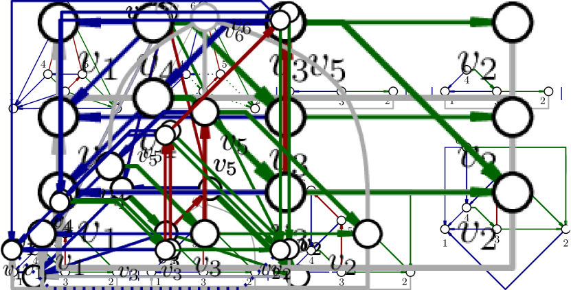
(b)

(c)

(d)

(e)

(f)

(g)

(h)

Figure 1: An illustration of our algorithm for triconnected $4$-planar graphs by an example: the octahedron graph. The underlying canonical order consists of the following partitions: $P_{0}=\{v_{1},v_{2}\}$, $P_{1}=\{v_{3}\}$, $P_{2}=\{v_{4}\}$, $P_{3}=\{v_{5}\}$ and $P_{4}=\{v_{6}\}$. (a) The direction and the coloring of the edges. (b) The corresponding reference edges (bold drawn); the edge $(v_{1},v_{2})$ of the first partition and the edge $(v_{1},v_{6})$ incident to the last (degree $4$) partition are ignored. (c) The placement of the first two partitions. (d) The placement of a singleton of degree $2$ incident to reference edge $(v_{4},v_{3})$ that is drawn bent. (e) The placement of a singleton of degree $3$ incident to reference edges $(v_{5},v_{4})$ and $(v_{5},v_{2})$ that are drawn bent. (f) The last singleton $v_{6}$ is not incident to reference edges. So, $(v_{6},v_{4})$, $(v_{5},v_{6})$ and $(v_{6},v_{2})$ must be drawn bend-less, which is not possible. (g) Vertex $v_{5}$ is translated upwards in the direction implied by the edge $(v_{3},v_{5})$ until one of the horizontal segments incident to $v_{5}$ is eliminated, which makes the placement of $v_{6}$ posible. (h) The final layout containing $(v_{2},v_{1})$ and $(v_{6},v_{1})$; the dotted edge can be drawn with a single bend.

2 Upper Bounds

In this section, we present upper bounds on the total number of bends for the classes of triconnected $4$-planar (Section 2.1), $5$-planar (Section 2.2) and $6$-planar (Section 2.3) graphs.

2.1 Triconnected 4-Planar Graphs.

Let $G=(V,E)$ be a triconnected $4$-planar graph. Before we proceed with the description of our approach, we need to define two useful notions. First, a vertical cut is a $y$-monotone continuous curve that crosses only horizontal segments and divides a drawing into a left and a right part; see e.g. [9]. Such a cut makes a drawing horizontally stretchable in the following sense: One can shift the right part of the drawing that is defined by the vertical cut further to the right while keeping the left part of the drawing in place and the result is a valid octilinear drawing. Similarly, one can define a horizontal cut.

Since $G$ has at most $2n$ edges, by Euler’s formula, it follows that $G$ has at most $n+2$ faces. In order to construct a drawing $\Gamma(G)$ of $G$, which has roughly at most $n+2$ bends, we also need to associate to each face of $G$ a so-called reference edge. This is done as follows. Let $\Pi=\{P_{0},\ldots,P_{m}\}$ be a canonical order of $G$ and assume that $\Gamma(G)$ is constructed incrementally by placing a new partition of $\Pi$ each time, so that the boundary of the drawing constructed so far is a $x$-monotone path. When placing a new partition $P_{k}\in\Pi$, $k=1,\ldots,m-1$, one or two bounded faces of $G$ are formed (note that we treat the last partition $P_{m}$ of $\Pi$ separately). More precisely, if $P_{k}$ is a chain or a singleton of degree $3$ in $G_{k}$, then only one bounded face is formed. Otherwise (that is, $P_{k}$ is a singleton of degree $4$ in $G_{k}$), two new bounded faces are formed. In both cases, each newly-formed bounded face consists of at least two edges incident to vertices of $P_{k}$ and at least one edge of $G_{k-1}$. In the former case, the reference edge of the newly-formed bounded face, say $f$, is defined as follows. If $f$ contains at least one green edge that belongs to $G_{k-1}$, then the reference edge of $f$ is the leftmost such edge (see Figure 2a and 2c). Otherwise, the reference edge of $f$ is the leftmost blue edge of $f$ that belongs to $G_{k-1}$ (see Figure 2b and 2d). In the case where $P_{k}$ is a singleton of degree $4$ in $G_{k}$, the reference edge of each of the newly formed faces is the edge of $G_{k-1}$ that is incident to the endpoint of the red edge involved. Observe that by definition a red edge cannot be a reference edge. For an example see Figure 1b.

(a)

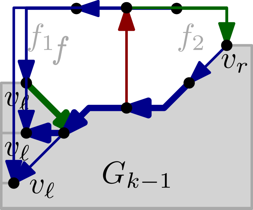
(b)

(c)

(d)

(e)

Figure 2: Illustration of the reference edge (bold drawn) in the case of: (a-b) a chain, (c-d) a singleton of degree $2$ in $G_{k}$ and (e) a singleton of degree $3$ in $G_{k}$.

As already stated, we will construct $\Gamma(G)$ in an incremental manner by placing one partition of $\Pi$ at a time. For the base, we momentarily neglect the edge $(v_{1},v_{2})$ of the first partition $P_{0}$ of $\Pi$ and we start by placing the second partition, say a chain $P_{1}=\{v_{3},\ldots,v_{|P_{1}|+2}\}$, on a horizontal line from left to right. Since by definition of $\Pi$, $v_{3}$ and $v_{|P_{1}|+2}$ are adjacent to the two vertices, $v_{1}$ and $v_{2}$, of the first partition $P_{0}$, we place $v_{1}$ to the left of $v_{3}$ and $v_{2}$ to the right of $v_{|P_{1}|+2}$. So, they form a single chain where all edges are drawn using horizontal line-segments that are attached to the east and west port at their endpoints. The case where $P_{1}$ is a singleton is analogous (assuming that $P_{1}$ is a chain of unit length). Assume now that we have already constructed a drawing for $G_{k-1}$ which has the following invariant properties:

1. The number of edges of $G_{k-1}$ with a bend is at most equal to the number of reference edges in $G_{k-1}$.

2. The north-west, north and north-east (south-west, south and south-east) ports of each vertex are occupied by incoming (outgoing) blue and green edges and by outgoing (incoming) red edges.

3. If a horizontal port of a vertex is occupied, then it is occupied either by an edge with a bend (to support vertical cuts) or by an edge of a chain.

4. A red edge is not on the outerface of $G_{k-1}$.

5. A blue (green, respectively) edge of $G_{k-1}$ is never incident to the north-west (north-east, respectively) port of a vertex of $G_{k-1}$.

6. From each reference edge on the outerface of $G_{k-1}$ one can devise a vertical cut through the drawing of $G_{k-1}$.

The base of our algorithm conforms with the aforementioned invariant properties. In the following, we will show how to add the next partition $P_{k}$ with $k<m$, so that all invariant properties are fulfilled. In our description, we will mainly describe the port assignment at each vertex that will always conform to IP-2–5, which fully specifies how each edge must be drawn (in other words, we describe the relative coordinates of the vertices). The exact coordinates can then be computed by adopting an approach similar to the one of Bekos et al. [2], since the base of each newly formed face is horizontally stretchable (follows from IP-6). Next, we consider the three main cases; see also Figure 1 for an example.

1. $P_{k}=\{v_{i}\}$ is a singleton of degree $2$ in $G_{k}$; see Figure 3a, 3b. Let $v_{\ell}$ and $v_{r}$ be the leftmost and rightmost neighbors of $v_{i}$ in $G_{k-1}$ (note that $v_{\ell}$ and $v_{r}$ are not necessarily neighboring). We claim that the north-east port of $v_{\ell}$ and the north-west port of $v_{r}$ cannot be simultaneously occupied. For a proof by contradiction, assume that the claim does not hold. Denote by $v_{\ell}\rightsquigarrow v_{r}$ the path from $v_{\ell}$ to $v_{r}$ at the outerface of $G_{k-1}$ (neglecting the direction of the edges). By IP-5, $v_{\ell}\rightsquigarrow v_{r}$ starts as blue from the north-east port of $v_{\ell}$ and ends as green at the north-west port of $v_{r}$. So, inbetween there is a vertex of the path $v_{\ell}\rightsquigarrow v_{r}$ which has a neighbor in $P_{j}$ for some $j\geq k$; a contradiction to the degree of $v_{i}$. Without loss of generality assume that the north-east port of $v_{\ell}$ is unoccupied. To draw the edge $(v_{i},v_{\ell})$, we distinguish two cases. If $(v_{i},v_{\ell})$ is the reference edge of a face, then we draw $(v_{i},v_{\ell})$ as a horizontal-diagonal combination from the west port of $v_{i}$ towards the north-east port of $v_{\ell}$. Otherwise, $(v_{i},v_{\ell})$ is drawn bend-less from the south-west port of $v_{i}$ towards the north-east port of $v_{\ell}$. To draw the edge $(v_{i},v_{r})$, again we distinguish two cases. If the north-west port at $v_{r}$ is unoccupied, then $(v_{i},v_{r})$ will use this port at $v_{r}$. Otherwise, $(v_{i},v_{r})$ will use the north port at $v_{r}$. In addition, if $(v_{i},v_{r})$ is the reference edge of a face, then $(v_{i},v_{r})$ will use the east port at $v_{i}$. Otherwise, the south-east port at $v_{i}$. The port assignment described above conforms to IP-2–5. Clearly, IP-1 also holds. IP-6 holds because the newly introduced edges that are reference edges have a horizontal segment, which inductively implies that vertical cuts through them are possible.

   

   (a)

   

   (b)

   

   (c)

   

   (d)

   

   (e)

   

   (f)

   

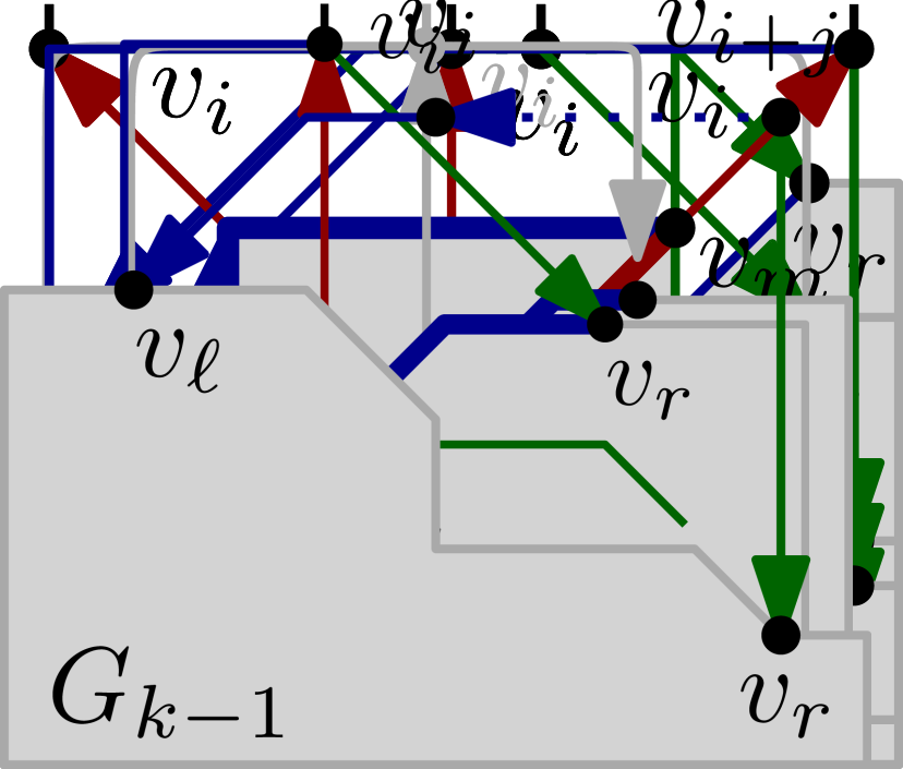
   (g)

   

   (h)

   

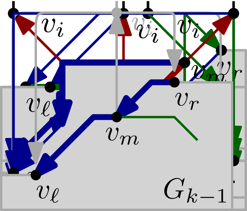
   (i)

   

   (j)

   Figure 3: Illustration of: (a-b) the case of a degree-$2$ singleton in $G_{k}$, (c) the case of a chain, (d-j) the case of a singleton of degree $3$ in $G_{k}$ (dotted segments can have zero length).

2. $P_{k}=\{v_{i},\ldots v_{i+j}\}$ with $j\geq 1$ is a chain. This case is similar to case C.1, as $P_{k}$ has also exactly two neighbors in $G_{k-1}$ (which we again denote by $v_{\ell}$ and $v_{r}$). The edges between $v_{i},\ldots,v_{i+j}$ will be drawn as horizontal segments connecting the west and east ports of the respective vertices; see Figure 3c. The edges $(v_{i},v_{\ell})$ and $(v_{i+j},v_{r})$ are drawn based on the rules of the case C.1 (e.g., in Figure 3c edge $(v_{i},v_{\ell})$ is a reference edge, while the edge $(v_{i+j},v_{r})$ is not). Hence, the port assignment still conforms to IP-2–IP-5. In addition, IP-1 and IP-6 hold, since all edges of the chain are horizontal.

3. $P_{k}=\{v_{i}\}$ is a singleton of degree $3$ in $G_{k}$. This is the most involved case. Let $v_{\ell}$ and $v_{r}$ be the leftmost and rightmost neighbors of $v_{i}$ in $G_{k-1}$ and let $v_{m}$ be the third neighbor of $v_{i}$ in $G_{k-1}$. By IP-2 and the degree restriction, the north port of $v_{m}$ is unoccupied. If the north-east port of $v_{\ell}$ and the north-west port of $v_{r}$ are simultaneously unoccupied, we proceed analogously to case C.1; see Figure 3d. Clearly, IP-1 and IP-6 hold. Consider now the more involved case, where the north-east port of $v_{\ell}$ is occupied and simultaneously $(v_{i},v_{\ell})$ is not a reference edge. Hence, by IP-6 $(v_{i},v_{\ell})$ must be drawn bend-less. Since the north-east port at $v_{\ell}$ is occupied, by IP-4 it follows that the edge at the north-east port of $v_{\ell}$ is not red. Therefore, by IP-2 and IP-5, the edge at the north-east port of $v_{\ell}$ is blue. This implies that the path $v_{\ell}\rightsquigarrow v_{m}$ at the outerface of $G_{k-1}$ consists of exclusively blue edges pointing towards $v_{\ell}$. Hence, by IP-5 the north-east port at $v_{m}$ is unoccupied. Edge $(v_{i},v_{\ell})$ can be drawn bend-less if the edge $(v_{i},v_{r})$ is a reference edge (that is, by IP-6 $(v_{i},v_{r})$ has a bend); see Figure 3e. In the case where the edge $(v_{i},v_{r})$ is not a reference edge (that is, none of $(v_{i},v_{\ell})$ and $(v_{i},v_{r})$ is a reference edge), we need a different argument. We further distinguish two sub-cases.

   C.3.1: The edge incident to $v_{m}$ on the path $v_{m}\rightsquigarrow v_{r}$ on the outerface of $G_{k-1}$ is green(we cope with the case where this edge is blue later). By definition, the blue (green) edge of $v_{\ell}\rightsquigarrow v_{m}$ ($v_{m}\rightsquigarrow v_{r}$) incident to $v_{m}$ is a reference edge and by IP-6 has a bend. Our aim is to “eliminate” one of these bends and draw one of the edges $(v_{i},v_{\ell})$ or $(v_{i},v_{r})$ with a bend and the other one bend-less. So, IP-1 still holds. In this case, $v_{m}$ may or may not be incident to another red edge in $G_{k-1}$ (equivalently, $v_{m}$ is either of degree $4$ or $3$, respectively). Without loss of generality we assume that $v_{m}$ is incident to another red edge, say $(v_{m},v_{m}^{\prime})$, in $G_{k-1}$, that is, $v_{m}$ is of degree $4$. In this case, we translate $v_{m}$ upwards in the direction implied by the slope of the edge $(v_{m},v_{m}^{\prime})$, until one of the horizontal segments of the edges incident to $v_{m}$ on the outerface of $G_{k-1}$ is completely eliminated; see Figure 3f. The only case, where the aforementioned segment elimination is not possible, is when $(v_{m},v_{m}^{\prime})$ is vertical and the edges incident to $v_{m}$ at the outerface of $G_{k-1}$ are both horizontal-vertical combinations; see Figure 3g. In this particular case, however, by IP-2 it follows that either the north-west or the north-east port at $v_{m}^{\prime}$ is free. Since both edges incident to $v_{m}$ at the outerface of $G_{k-1}$ are bent, by IP-3 we can redraw $(v_{m}^{\prime},v_{m})$ so to be diagonal and then we proceed similarly to the previous case; see Figure 3h. Also, observe that the port assignment still conforms to IP-2–IP-5. C.3.2: The edge incident to $v_{m}$ on the path $v_{m}\rightsquigarrow v_{r}$ on the outerface of $G_{k-1}$ is blue.In this case, $v_{m}$ cannot be incident to another red edge. In the case where $v_{m}$ is of degree $3$, we proceed similar to the case C.3.1, where $v_{m}$ was of degree $3$. So, we now focus on the case where $v_{m}$ is of degree $4$. In this case, the fourth edge attached to $v_{m}$ can be either (outgoing) green or (incoming) blue. In the former case, this edge is a reference edge. In the latter case, it is part of a chain. In both cases, however, this edge has a horizontal segment; see Figure 3i. Hence, we can translate $v_{m}$ horizontally to the left so to eliminate the bend of the edge incident to $v_{m}$ on the path $v_{\ell}\rightsquigarrow v_{m}$; see Figure 3j. Note that all invariant properties are fulfilled once $v_{i}$ is drawn.

Note that the coordinates of the newly introduced vertices are determined by the shape of the edges connecting them to $G_{k-1}$. If there is not enough space between $v_{\ell}$ and $v_{r}$ to accommodate the new vertices, IP-6 allows us to stretch the drawing horizontally using the reference edge of the newly formed face.

To complete the description of our algorithm, it remains to cope with the last partition $P_{m}=\{v_{n}\}$ and describe how to draw the edge $(v_{1},v_{2})$ of the first partition $P_{0}$ of $\Pi$. If $v_{n}$ is of degree $3$, we cope with $P_{m}$ as being an ordinary singleton. However, if $v_{n}$ is of degree $4$, then we momentarily ignore the edge $(v_{n},v_{1})$ of $P_{m}$ and proceed to draw the remaining edges incident to $v_{n}$, assuming that $P_{m}$ is again an ordinary singleton. The edge $(v_{n},v_{1})$ can be drawn afterwards using two bends in total. Finally, since by construction $v_{1}$ and $v_{2}$ are horizontally aligned, we can draw the edge $(v_{1},v_{2})$ with a single bend, emanating from the south-east port of $v_{1}$ towards the south-west port of $v_{2}$.

Theorem 1.

Let $G$ be a triconnected $4$-planar graph with $n$ vertices. A planar octilinear drawing $\Gamma(G)$ of $G$ with at most $n+5$ bends can be computed in $O(n)$ time.

Proof.

By IP-1, all bends of $\Gamma(G)$ are in correspondence with the reference edges of $G$, except for the bends of the edges $(v_{1},v_{2})$ and $(v_{n},v_{1})$. Since the number of reference edges is at most $n+2$ and the edges $(v_{1},v_{2})$ and $(v_{n},v_{1})$ require $3$ additional bends, the total number of bends of $\Gamma(G)$ does not exceed $n+5$. The linear running time follows from the observation that we can use the shifting method of Kant [13] to compute the actual coordinates of the vertices of $G$, since in the canonical order the y-coordinates of the vertices that have been placed at some particular step do not change in subsequent steps (following a similar approach as in [2]). ∎

2.2 Triconnected 5-Planar Graphs.

Our algorithm for triconnected $5$-planar graphs is an extension of the corresponding algorithm of Bekos et al. [2], which computes for a given triconnected $5$-planar graph $G$ on $n$ vertices a planar octilinear drawing $\Gamma(G)$ of $G$ with at most one bend per edge. Since $G$ cannot have more than $5n/2$ edges, it follows that the total number of bends of $\Gamma(G)$ is at most $5n/2$. However, before we proceed with the description of our extension, we first provide some insights into this algorithm, which is based on a canonical order $\Pi$ of $G$. Central are IP-2 and IP-4 of the previous section and the so-called stretchability invariant, according to which all edges on the outerface of the drawing constructed at some step of the canonical order have a horizontal segment and therefore one can devise corresponding vertical cuts to horizontally stretch the drawing. We claim that we can appropriately modify this algorithm, so that all red edges of $\Pi$ are bend-less.

Since we seek to draw all red edges of $\Pi$ bend-less, our modification is limited to singletons. So, let $P_{k}=\{v_{i}\}$ be a singleton of $\Pi$. The degree restriction implies that $v_{i}$ has at most two incoming red edges (we also assume that $P_{k}$ is not the last partition of $\Pi$, that is $k\neq m$). We first consider the case where $v_{i}$ has exactly one incoming red edge, say $e=(v_{j},v_{i})$, with $j<i$. By construction, $e$ must be attached to one of the northern ports of $v_{j}$ (that is, north-west, north or north-east). On the other hand, $e$ can be attached to any of the southern ports of $v_{i}$, as $e$ is its only incoming red edge. This guarantees that $e$ can be drawn bend-less.

Consider now the more involved case, where $v_{i}$ has exactly two incoming red edges, say $e=(v_{j},v_{i})$ and $e^{\prime}=(v_{j^{\prime}},v_{i})$ and assume without loss of generality that $v_{j}$ is to the left of $v_{j^{\prime}}$ in the drawing of $G_{k-1}$. We distinguish three cases based on the available ports of $v_{j}$:

1. The north-east port of $v_{j}$ is unoccupied: In this case, $e$ emanates from the north-east port of $v_{j}$ and leads to the south-west port of $v_{i}$ (recall that all southern ports of singleton $v_{i}$ are dedicated for incoming red edges; in this case $e$ and $e^{\prime}$). If the north-west or the north port of $v_{j^{\prime}}$ is unoccupied, then $e^{\prime}$ can be easily drawn bend-less. In the former case, $e^{\prime}$ emanates from the north-west port of $v_{j^{\prime}}$ and leads to the south-east port of $v_{i}$. In the latter case, $e^{\prime}$ emanates from the north port of $v_{j^{\prime}}$ and leads to the south port of $v_{i}$. Hence, the aforementioned port assignment fully specifies the position of $v_{i}$. It remains to consider the case, where neither the north-west nor the north port of $v_{j^{\prime}}$ is unoccupied, that is, the north-east port of $v_{j^{\prime}}$ is unoccupied. By our coloring scheme and IP-2, $v_{j^{\prime}}$ has already two incoming green edges, say $e_{g}$ and $e_{g}^{\prime}$, and $e^{\prime}$ is the last edge to be attached at $v_{j^{\prime}}$; see Figure 4a. Therefore, there is no other (bend-less) red edge involved. We proceed by shifting $v_{j^{\prime}}$ up in a way that makes all northern ports of $v_{j^{\prime}}$ unoccupied; see Figure 4b. Note that we may have to use a second bend on the outgoing blue edge of $v_{j^{\prime}}$ (in order to maintain the stretchability invariant), but on the other hand we can eliminate one bend from the second green edge $e_{g}^{\prime}$; see Figure 4b. So, the total number of bends remains unchanged. In addition, the endpoints of both $e_{g}$ and $e_{g}^{\prime}$ that are opposite to $v_{j^{\prime}}$ may have to be moved horizontally to allow $e_{g}$ and $e_{g}^{\prime}$ to be drawn planar, but by the stretchability invariant we are guaranteed that this is always possible. Finally, the stretchability invariant is maintained, since each edge besides the red ones contains a horizontal segment.

   

   (a)

   

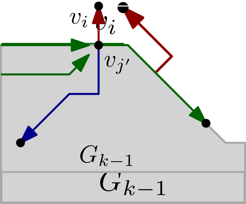
   (b)

   Figure 4: (a) $e^{\prime}=(v_{j^{\prime}},v_{i})$ cannot be drawn bend-less. (b) Shifting $v_{j^{\prime}}$ up resolves the problem.

2. The north-east port of $v_{j}$ is occupied, while its north port is unoccupied: In this case, $e$ emanates from the north port of $v_{j}$ and leads to the south port of $v_{i}$ (that is, $v_{i}$ and $v_{j}$ are vertically aligned). We now claim that the north-west port of $v_{j^{\prime}}$ is unoccupied. For the sake of contradiction, assume that the claim is not true. By our coloring scheme, the edge attached at the north-west port of $v_{j^{\prime}}$ is green, which implies that there must exist a path $v_{j}\rightsquigarrow v_{j^{\prime}}$ at the outerface face of $G_{k-1}$ whose first edge is blue at the north-east port of $v_{j}$ and its last edge is green at the north-west port of $v_{j^{\prime}}$. So, path $v_{j}\rightsquigarrow v_{j^{\prime}}$ has a vertex which has a neighbor in $P_{\kappa}$ for some $\kappa\geq k$. Since $v_{i}$ is the only such candidate, the contradiction follows from the degree of $v_{i}$. Hence, the north-west port of $v_{j^{\prime}}$ is unoccupied and therefore we can draw $e^{\prime}$ without bends by using the south-east port of $v_{i}$ and the north-west port of $v_{j^{\prime}}$, as desired.

3. Only the north-west port of $v_{j}$ is unoccupied: We can reduce this case to case C.1 by applying an operation symmetric to the one of Figure 4a on vertex $v_{j}$. This will result in a configuration where all northern ports of $v_{j}$ (including the north-east) are unoccupied.

Theorem 2.

Let $G$ be a triconnected $5$-planar graph with $n$ vertices. A planar octilinear drawing $\Gamma(G)$ of $G$ with at most $2n-2$ bends can be computed in $O(n)$ time.

Proof.

From our extension, it follows that the only edges of $\Gamma(G)$ that have a bend are the blue and the green ones and possibly the third incoming red edge of vertex $v_{n}$ of the last partition $P_{m}$ of $\Pi$. Now, recall that the blue subgraph is a spanning tree of $G$, while the green one is a forest on the vertices of $G$. So, in the worst case the green subgraph is a tree on $n-1$ vertices of $G$ (by construction the green subgraph cannot be incident to the first vertex $v_{1}$ of $\Pi$). Therefore, at most $2n-2$ edges of $\Gamma(G)$ have a bend. In addition, the running time remains linear since the shifting technique can still be applied. This is because once a vertex has been placed its $y$-coordinate does not change anymore, except for the special case of two red edges (cases C.1 and C.3), which does not influence the overall running time, since it can occur at most once per vertex. ∎

2.3 Triconnected 6-Planar Graphs.

In this section, we present an algorithm that based on a canonical order $\Pi=\{P_{0},P_{1},\ldots,P_{m}\}$ of a given triconnected $6$-planar graph $G=(V,E)$ results in a drawing $\Gamma(G)$ of $G$, in which each edge has at most two bends. Hence, in total $\Gamma(G)$ has $6n-12$ bends. Then, we show how one can appropriately adjust the produced drawing to reduce the total number of bends.

(a)

(b)

(c)

(d)

(e)

(f)

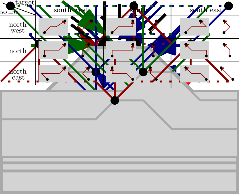
(g)

(h)

(i)

(j)

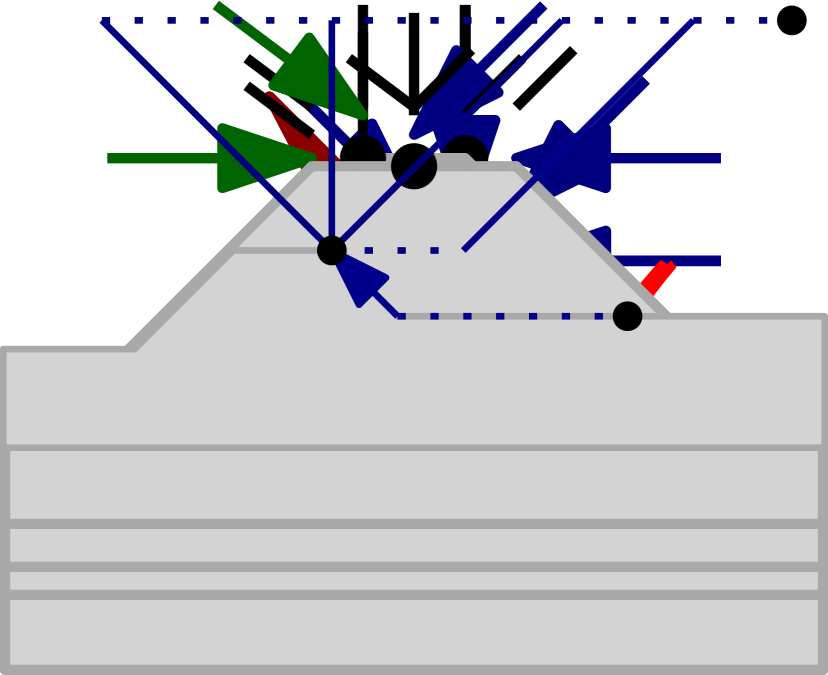
(k)

Figure 5: (a)-(f) Illustration of the port assignment computed by Algorithm 1. (g)-(k) Different segment combinations with at most two bends (horizontal segments are drawn dotted)

1

input : A vertex $v$ of a triconnected $6$-planar graph.

output : The port assignment of the edges around $v$, according to the following rules.

1. The incoming blue edges of $v$ occupy consecutive ports in counterclockwise order

around $v$ starting from:

1. the south-east port of $v$, if $\mathrm{indeg}_{\mathrm{b}}(v)+\mathrm{outdeg}_{\mathrm{r}}(v)=5$; see Figure 5a.

2. the east port of $v$, if $\mathrm{indeg}_{\mathrm{b}}(v)+\mathrm{outdeg}_{\mathrm{r}}(v)=4$; see Figure 5b.

3. the east port of $v$, if $\mathrm{outdeg}_{\mathrm{g}}(v)=0$ and (a),(b) do not hold; see Figure 5c.

4. the north-east port of $v$, otherwise; see Figure 5d.

The outgoing red edge occupies the counterclockwise next unoccupied port, if $v$ has

at least one incoming blue edge. Otherwise, the north-east port of $v$.

The incoming green edges of $v$ occupy consecutive ports in clockwise order around $v$ starting from:

1. the west port of $v$, if $\mathrm{indeg}_{\mathrm{g}}(v)+\mathrm{outdeg}_{\mathrm{r}}(v)+\mathrm{indeg}_{\mathrm{b}}(v)\geq 4$; see Figure 5e.

2. the north-west port of $v$, otherwise; see Figure 5f.

The outgoing blue edge of $v$ occupies the west port of $v$, if it is unoccupied;

otherwise, the south-west port of $v$.

The outgoing green edge of $v$ occupies the east port of $v$, if it is unoccupied;

otherwise, the south-east port of $v$.

The incoming red edges of $v$ occupy consecutively in counterclockwise direction the south-west, south and south-east ports of $v$ starting from the first available.

Algorithm 1 PortAssignment(v)

Algorithm 1 describes rules R1 - R6 to assign the edges to the ports of the corresponding vertices. It is not difficult to see that all port combinations implied by these rules can be realized with at most two bends, so that all edges have a horizontal segment (which makes the drawing horizontally stretchable): (i) a blue edge emanates from the west or south-west port of a vertex (by rule R4) and leads to one of the south-east, east, north-east, north or north-west ports of its other endvertex (by rule R1); see Figure 5g and 5h, (ii) a green edge emanates from the east or south-east port of a vertex (by rule R5) and leads to one of the west, north-west, north or north-east ports of its other endvertex (by rule R3); see Figure 5i and 5j, (iii) a red edge emanates from one of the north-west, north, north-east ports of a vertex (by rule R2) and leads to one of the south-west, south, south-east ports of its other endvertex (by rule R6); see Figure 5k.

Hence, the shape of each edge is completely determined. To compute the actual drawing $\Gamma(G)$ of $G$, we follow an incremental approach according to which one partition (that is, a singleton or a chain) of $\Pi$ is placed at a time, similar to Kant’s approach [12] and the $4$- or $5$-planar case. Each edge is drawn based on its shape, while the horizontal stretchability ensures that potential crossings can always be eliminated. Note additionally that we adopt the leftist canonical order [1], according to which the leftmost partition is chosen to be placed, when there exist two or more candidates. Since each edge has at most two bends, $\Gamma(G)$ has at most $6n-12$ bends in total.

In the following, we reduce the total number of bends. This is done in two steps. In the first step, we show that all red edges can be drawn with at most one bend each. Recall that a red edge emanates from one of the north-west, north, north-east ports of a vertex and leads to one of the south-west, south, south-east ports of its other-endvertex. So, in order to prove that all red edges can be drawn with at most one bend each, we have to consider in total nine cases, which are illustrated in Figure 6. It is not difficult to see that in each of these cases, the red edge can be drawn with at most one bend. Note that the absence of horizontal segments at the red edges does not affect the stretchability of $\Gamma(G)$, since each face of $\Gamma(G)$ has at most two such edges (which both “point upward” at a common vertex). Since a red edge cannot be incident to the outerface of any intermediate drawing constructed during the incremental construction of $\Gamma(G)$, it follows that it is always possible to use only horizontal segments (of blue and green edges) to define vertical cuts, thus, avoiding all red edges.

Figure 6: Red edges can be redrawn with one bend (in gray boxes we show their initial 2-bends shapes)

The second step of our bend reduction is more involved. Our claim is that we can “save” two bends per vertex, which yields a reduction by roughly $2n$ bends in total. To prove the claim, consider an arbitrary vertex $u\in V$ of $G$. Our goal is to prove that there always exist two edges incident to $u$, which can be drawn with only one bend each. By rules R3 and R4, it follows that the west port of vertex $u$ is always occupied, either by an incoming green edge (by rule R3) or by a blue outgoing edge (by rule R4; $u\neq v_{1}\in P_{0}$). Analogously, the east port of vertex $u$ is always occupied, either by a blue incoming edge (by rules R1 and R2) or by an outgoing green edge (by rule R5). Let $(u,v)\in E$ be the edge attached at the west port of $u$ (symmetrically we cope with the edge that is attached at the east port of $u$). If edge $(u,v)$ is attached to a non-horizontal port at $v$, then $(u,v)$ is by construction drawn with one bend (regardless of its color; see Figure 5g and 5i) and our claim follows.

It remains to consider the case where edge $(u,v)$ is attached to a horizontal port at $v$. Assume first that edge $(u,v)$ is blue (we will discuss the case where edge $(u,v)$ is green later). By Algorithm 1, it follows that edge $(u,v)$ is either the first blue incoming edge attached at $v$ (by rules R1b and R1c) or the second one (by rule R1a). We consider each of these cases separately. In rule R1c, observe that edge $(u,v)$ is part of a chain (because $\mathrm{outdeg}_{\mathrm{g}}(u)=0$). Hence, when placing this chain in the canonical order, we will place $u$ directly to the right of $v$. This implies that $(u,v)$ will be drawn as a horizontal line segment (that is, bend-less). Similarly, we cope with rule R1b, when additionally $\mathrm{outdeg}_{\mathrm{g}}(u)=0$. So, there are still two cases to consider: rule R1a and rule R1b, when additionally $\mathrm{outdeg}_{\mathrm{g}}(u)=1$; see the left part of Figure 7. In both cases, the current degree of vertex $u$ is $3$ and vertex $v$ (and other vertices that are potentially horizontally-aligned with $v$) must be shifted diagonally up, when $u$ is placed based on the canonical order, such that $(u,v)$ is drawn as a horizontal line segment (that is, bend-less; see the right part of Figure 7). Note that when $v$ is shifted up, vertex $v$ and all vertices that are potentially horizontally-aligned with $v$ are also of degree $3$, since otherwise one of these vertices would not have a neighbor in some later partition of $\Pi$, which contradicts the definition of $\Pi$.

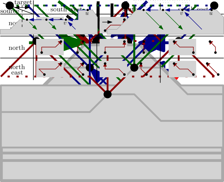
Figure 7: Aligning vertices $u$ and $v$.

We complete our case analysis with the case where edge $(u,v)$ is green. By rule R3a, it follows that $(u,v)$ is the first green incoming edge attached at $u$. In addition, when $(u,v)$ is placed based on the canonical order, there is no red outgoing edge attached at $u$ (otherwise $u$ would not be at the outerface of the drawing constructed so far). The leftist canonical order also ensures that there is no blue incoming edge at $u$ drawn before $(u,v)$. Hence, vertex $u$ is of degree two, when edge $(u,v)$ is placed. Hence, it can be shifted up (potentially with other vertices that are horizontally-aligned with $u$), such that $(u,v)$ is drawn as a horizontal line segment (that is, bend-less). We summarize our approach in the following theorem.

Theorem 3.

Let $G$ be a triconnected $6$-planar graph with $n$ vertices. A planar octilinear drawing $\Gamma(G)$ of $G$ with at most $3n-8$ bends can be computed in $O(n^{2})$ time.

Proof.

Before the two bend-reduction steps, $\Gamma(G)$ contains at most $6n-12$ bends. In the first reduction step, all red edges are drawn with one bend. Hence, $\Gamma(G)$ contains at most $5n-9$ bends. In the second reduction step, we “save” two bends per vertex (except for $v_{1}\in P_{0}$, which has no outgoing blue edge), which yields a reduction by $2n-1$ bends. Therefore, $\Gamma(G)$ contains at most $3n-8$ bends in total. On the negative side, we cannot keep the running time of our algorithm linear. The reason is the second reduction step, which yields changes in the $y$-coordinates of the vertices. In the worst case, however, quadratic time suffices. ∎

Note that there exist $6$-planar graphs that do not admit planar octilinear drawings with at most one bend per edge [2]. Theorem 3 implies that on average one bend per edge suffices.

3 Lower Bounds

In this section, we present lower bounds on the total number of bends for the classes of triconected $4$-, $5$- and $6$-planar graphs.

3.1 4-Planar Graphs.

We start our study with the case of $4$-planar graphs. Our main observation is that if a $3$-cycle $\mathcal{C}_{3}$ of a graph has at least two vertices, with at least one neighbor in the interior of $\mathcal{C}_{3}$ each, then at least one edge of $\mathcal{C}_{3}$ must contain a bend, since the sum of the interior angles at the corners of $\mathcal{C}_{3}$ exceeds $180^{\circ}$. In fact, elementary geometry implies that a $k$-cycle, say $\mathcal{C}_{k}$ with $k\geq 3$, whose vertices have $\sigma\geq 0$ neighbors in the interior of $\mathcal{C}_{k}$ requires (at least) $\max\{0,\lceil(\sigma-3k+8)/3\rceil\}$ bends. Therefore, a bend is necessary. Now, refer to the $4$-planar graph of Figure 8a, which contains $n/3$ nested triangles, where $n$ is the number of its vertices. It follows that this particular graph requires at least $n/3-1$ bends in total.

(a) A $4$-planar graph

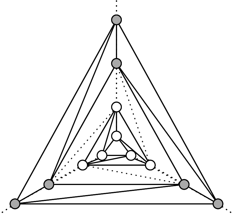
(b) A $5$-planar graph

(c) A $6$-planar graph

Figure 8: Planar graphs of different degrees that require (a) $n/3-1$, (b) $2n/3-2$ and (c) $4n/3-6$ bends.

3.2 5- and 6-Planar Graphs.

For $5$- and $6$-planar graphs, our proof becomes more complex. For these classes of graphs, we follow an approach inspired by Tamassia’s min-cost flow formulation [19] for computing bend-minimum representations of embedded planar graphs of bounded degree. Since it is rather difficult to implement this algorithm in the case where the underlying drawing model is not the orthogonal model, we developed an ILP instead. Recall that a representation describes the “shape” of a drawing without specifying its exact geometry. This is enough to determine a lower bound on the number of bends, even if a bend-optimal octilinear representation may not be realizable by a corresponding (planar) octilinear drawing.

In our formulation, variable $\alpha(u,v)\cdot 45^{\circ}$ corresponds to the angle formed at vertex $u$ by edge $(u,v)$ and its cyclic predecessor around vertex $u$. Hence, $1\leq\alpha(u,v)\leq 8$. Since the sum of the angles around a vertex is $360^{\circ}$, it follows that $\sum_{v\in N(u)}a(u,v)=8$. Given an edge $e=(u,v)$, variables $\ell_{45}(u,v)$, $\ell_{90}(u,v)$ and $\ell_{135}(u,v)$ correspond to the number of left turns at $45^{\circ}$, $90^{\circ}$ and $135^{\circ}$ when moving along $(u,v)$ from vertex $u$ towards vertex $v$. Similarly, variables $r_{45}(u,v)$, $r_{90}(u,v)$ and $r_{135}(u,v)$ are defined for right turns. All aforementioned variables are integer lower-bounded by zero. For a face $f$, we assume that its edges are directed according to the clockwise traversal of $f$. This implies that each (undirected) edge of the graph appears twice in our formulation. For reasons of symmetry, we require $\ell_{45}(u,v)=r_{45}(v,u)$, $\ell_{90}(u,v)=r_{90}(v,u)$ and $\ell_{135}(u,v)=r_{135}(v,u)$. Since the sum of the angles formed at the vertices and at the bends of a bounded face $f$ equals to $180^{\circ}\cdot(p(f)-2)$, where $p(f)$ denotes the total number of such angles, it follows that $\sum_{(u,v)\in E(f)}\alpha(u,v)+(\ell_{45}(u,v)+\ell_{90}(u,v)+\ell_{135}(u,v))-(r_{45}(u,v)+r_{90}(u,v)+r_{135}(u,v))=4a(f)-8$, where $a(f)$ denotes the total number of vertex angles in $f$, and, $E(f)$ the directed arcs of $f$ in its clockwise traversal. If $f$ is unbounded, the respective sum is increased by $16$. Of course, the objective is to minimize the total number of bends over all edges, or, equivalently $\min\sum_{(u,v)\in E}\ell_{45}(u,v)+\ell_{90}(u,v)+\ell_{135}(u,v)+r_{45}(u,v)+r_{90}(u,v)+r_{135}(u,v)$.

Now, consider the $5$-planar graph of Figure 8b and observe that each “layer” of this graph consist of six vertices that form an octahedron (solid-drawn), while octahedrons of consecutive layers are connected with three edges (dotted-drawn). Using our ILP formulation, we prove that each octahedron subgraph requires at least $4$ bends, when drawn in the octilinear model (except for the innermost one for which we can guarantee only two bends). This implies that $2n/3-2$ bends are required in total to draw the graph of Figure 8b. For the $6$-planar case, we apply our ILP approach to a similar graph consisting of nested octahedrons that are connected by six edges each; see Figure 8c. This leads to a better lower bound of $4n/3-6$ bends, as each octahedron except for the innermost one requires $8$ bends. Summarizing we have:

Theorem 4.

There exists a class $G_{n,k}$ of triconnected embedded $k$-planar graphs, with $4\leq k\leq 6$, whose octilinear drawings require at least: (i) $n/3-1$bends, if $k=4$, (ii) $2n/3-2$bends, if $k=5$ and (iii) $4n/3-6$bends, if $k=6$.

4 Conclusions

In this paper, we studied bounds on the total number of bends of octilinear drawings of triconnected planar graphs. We showed how one can adjust an algorithm of Keszegh et al. [14] to derive an upper bound of $4n-10$ bends for general $8$-planar graphs. Then, we improved this general bound and previously-known ones for the classes of triconnected $4$-, $5$- and $6$-planar graphs. For these classes of graphs, we also presented corresponding lower bounds.
We mention two major open problems in this context. The first one is to extend our results to biconnected and simply connected graphs and to further tighten the bounds. Since our drawing algorithms might require super-polynomial area (cf. arguments from [2]), the second problem is to study trade-offs between the total number of bends and the required area.

References

- [1] M. Badent, U. Brandes, and S. Cornelsen. More canonical ordering. Journal of Graph Algorithms and Applications, 15(1):97–126, 2011.
- [2] M. A. Bekos, M. Gronemann, M. Kaufmann, and R. Krug. Planar octilinear drawings with one bend per edge. Journal of Graph Algorithms and Applications, 19(2):657–680, 2015.
- [3] T. C. Biedl. New lower bounds for orthogonal graph drawings. In F. J. Brandenburg, editor, Graph Drawing, volume 1027 of LNCS, pages 28–39. Springer, 1996.
- [4] T. C. Biedl and G. Kant. A better heuristic for orthogonal graph drawings. Computational Geometry, 9(3):159–180, 1998.
- [5] H. L. Bodlaender and G. Tel. A note on rectilinearity and angular resolution. Journal of Graph Algorithms and Applications, 8(1):89–94, 2004.
- [6] H. De Fraysseix, J. Pach, and R. Pollack. How to draw a planar graph on a grid. Combinatorica, 10(1):41–51, 1990.
- [7] E. Di Giacomo, G. Liotta, and F. Montecchiani. The planar slope number of subcubic graphs. In A. Pardo and A. Viola, editors, LATIN, volume 8392 of LNCS, pages 132–143. Springer, 2014.
- [8] S. Felsner. Schnyder woods or how to draw a planar graph? In Geometric Graphs and Arrangements, Advanced Lectures in Mathematics, pages 17–42. Vieweg/Teubner Verlag, 2004.
- [9] U. Fössmeier, C. Hess, and M. Kaufmann. On improving orthogonal drawings: The 4M-algorithm. In S. Whitesides, editor, Graph Drawing, volume 1547 of LNCS, pages 125–137. Springer, 1998.
- [10] A. Garg and R. Tamassia. On the computational complexity of upward and rectilinear planarity testing. SIAM Journal on Computing, 31(2):601–625, 2001.
- [11] S.-H. Hong, D. Merrick, and H. A. D. do Nascimento. Automatic visualisation of metro maps. Journal of Visual Languages and Computing, 17(3):203–224, 2006.
- [12] G. Kant. Drawing planar graphs using the lmc-ordering. In FOCS, pages 101–110. IEEE, 1992.
- [13] G. Kant. Hexagonal grid drawings. In E. W. Mayr, editor, WG, volume 657 of LNCS, pages 263–276. Springer, 1992.
- [14] B. Keszegh, J. Pach, and D. Pálvölgyi. Drawing planar graphs of bounded degree with few slopes. SIAM Journal of Discrete Mathematics, 27(2):1171–1183, 2013.
- [15] Y. Liu, A. Morgana, and B. Simeone. A linear algorithm for 2-bend embeddings of planar graphs in the two-dimensional grid. Discrete Applied Mathematics, 81(1-3):69–91, 1998.
- [16] M. Nöllenburg. Automated drawings of metro maps. Technical Report 2005-25, Fakultät für Informatik, Universität Karlsruhe, 2005.
- [17] M. Nöllenburg and A. Wolff. Drawing and labeling high-quality metro maps by mixed-integer programming. IEEE Transactions on Visualization and Computer Graphics, 17(5):626–641, 2011.
- [18] J. M. Stott, P. Rodgers, J. C. Martinez-Ovando, and S. G. Walker. Automatic metro map layout using multicriteria optimization. IEEE Transactions on Visualization and Computer Graphics, 17(1):101–114, 2011.
- [19] R. Tamassia. On embedding a graph in the grid with the minimum number of bends. SIAM Journal of Computing, 16(3):421–444, 1987.
- [20] R. Tamassia, I. G. Tollis, and J. S. Vitter. Lower bounds for planar orthogonal drawings of graphs. Information Processing Letters, 39(1):35–40, 1991.