$f(T,\mathcal{T})$ Cosmological Models in Phase Space

Abstract

In this paper we explore $f(T,\mathcal{T})$, where $T$ and $\mathcal{T}$ denote the torsion scalar and the trace of the energy-momentum tensor respectively. We impose the covariant conservation to the energy-momentum tensor and obtain a cosmological $f(T,\mathcal{T})$ respectively. We impose the covariant conservation to the energy-momentum tensor and obtain a cosmological $f(T,\mathcal{T})$ model. Then, we study the stability of the obtained model for power-law and de Sitter solutions and our result show that the model can be stable for some values of the input parameters, for both power-law and de Sitter solutions.

I Introduction

Nowadays the current acceleration of the expansion of the universe is widely confirmed by several independent cosmological observational data as Cosmic Microwave Background Radiation (CMBR) Spergel and the Sloan Digital Sky Survey (SDSS) Adelman . This stage of the universe is explained in the literature through two approaches. The first assumes that the universes if filled by an exotic ith negative pressure, named dark energy known as the responsible of this acceleration of the universe. The second approach, instead of assuming an exotic component, consists to modify the GR by changing the usual Einstein-Hilbert gravitational term, and various theories have been developed in this way and based on the Levi-Civita’s connections, as ( $f(R)$, $f(R,\mathcal{T})$ ma1 -ma6 , $f(G)$) mj1 -mj5 where $R$ denotes the curvature scalar, $\mathcal{T}$ the trace of the energy-momentum tensor and $G$ the Gauss-Bonnet invariant defined by $G=R^{2}-4R_{\mu\nu}R^{\mu\nu}+R_{\mu\nu\ lambda\sigma}R^{\mu\nu\lambda\sigma}$. There exists another type theory based the weitzenbock’s connections, equivalent to GR, called Tele-parallel Theory $(TT)$. This theory has been introduced by Ferraro et al st1 where they explained the UV modifications to the $TT$ and also the inflation. After this, Ferraro and Bengochea st1 have consider the same model to describe the dark energy. other works can be found in st2 - st41 . In the same, modified versions of this theory have been developed and the one to which we are interested in this paper the $f(T,\mathcal{T})$, $T$ and $\mathcal{T}$ being the torsion scalar and the trace of the energy-momentum tensor, respectively. Specifically, this theory can be view as an homologue to $f(,\mathcal{T})$. Beside several works developed within $f(T,\mathcal{T})$ sala1 - sala4 , we can note the one undertaken by Alvarenga and collaborators papierdiego , where they search for the model for which the covariant conservation of the energy-momentum tensor is realized. In that paper they investigate the dynamics of scalar perturbations about the obtained model and focused they attention to the sub-Hubble modes and show that through the quasi-static approximation the result are very different from the ones derived in the frame of concordance $\Lambda CDM$, constraining the validity of this kind of model.

In this paper we are interested to the coincidence cosmic problem and search for the $f(T,\mathcal{T})$ model according to what the tress tensor is conserved. In order to obtain a consistent model, we explore the dynamics and stability about the obtained model. To reach our goal, we assume that it possible to have anti-gravity interactions between the dark energy and the matter because of their unknown nature. We also introduce arbitrarily the terms of interaction between these components because we have not sure of the form of interaction between them. We realize a system of three dynamic equations which take into account the dark energy, the dark matter and the ordinary matter. Consequently, we reconstruct four models and we show that the dynamic equations have two possible attractive solutions namely the phase dominated by the dark matter and that dominated by the dark energy. During this investigation, we have realized that some dynamic systems are unstable; meaning that a model provides that everything disappear in the Universe and leads to an Universe more and more poor in energy. Other models show that the Universe should be filled by dark energy. Another important feature emerging from this work is the stability study of $\Lambda$CDM model under consideration by considering two interesting cosmological solutions i.e the power-law and the de Sitter solutions. We have analyzed the constrains on the input parameters and as results, we have found that the stability is always realized.

This paper is organized as follows: In Sec II we have reconstructed a model by vanishing the covariant derived of energy-momentum tensor. The stability of the obtained critical points of the dynamic systems has been explored in Sec III and the perturbation functions have been determined within the model under consideration in Sec VI. The Sec IV is devoted to cosmological dynamic study of the considered model. Finally, we have ended our investigation by a conclusion in Sec VII.

II Generality on $f(T,\mathcal{T})$ gravity within FLRW Cosmology

The modified theories of Tele-Parallel gravity are those for which the scalar torsion of Tele-Parallel action is substituted by an arbitrarily function of this latter. As it is done in Tele-Parallel, the modified versions of this theory are also described by the orthonormal tetrads which components are defined on the tangent space of each point of the manifold. The line element is written as

$$ds^{2}=g_{\mu\nu}dx^{\mu}dx^{\nu}=\eta_{ij}\theta^{i}\theta^{j}\,,$$ (1)

with the following definitions

$$d^{\mu}=e_{i}^{\;\;\mu}\theta^{i};\,\quad\theta^{i}=e^{i}_{\;\;\mu}dx^{\mu}.$$ (2)

Note that $\eta_{ij}=diag(1,-1,-1,-1)$ is the Minkowskian metric and the $\{e^{i}_{\;\mu}\}$ are the components of the tetrad which satisfy the following identity:

$$e^{\;\;\mu}_{i}e^{i}_{\;\;\nu}=\delta^{\mu}_{\nu},\quad e^{\;\;i}_{\mu}e^{\mu}_{\;\;j}=\delta^{i}_{j}.$$ (3)

In General Relativity, one use the following Levi-Civita’s connection which preserves the curvature whereas the torsion vanishes

$$\overset{\circ}{\Gamma}{}_{\;\;\mu\nu}^{\rho}=\frac{1}{2}g^{\rho\sigma}\left(\partial_{\nu}g_{\sigma\mu}+\partial_{\mu}g_{\sigma\nu}-\partial_{\sigma}g_{\mu\nu}\right)\;,$$ (4)

But in the Tele-Parallel theory and its modified version, one keeps the scalar torsion by using Weizenbock’s connection defined as:

$$\Gamma^{\lambda}_{\mu\nu}=e^{\;\;\lambda}_{i}\partial_{\mu}e^{i}_{\;\;\nu}=-e^{i}_{\;\;\mu}\partial_{\nu}e_{i}^{\;\;\lambda}.$$ (5)

From this connection, one obtains the geometric objects. The first is the torsion defined by

$$T^{\lambda}_{\;\;\;\mu\nu}=\Gamma^{\lambda}_{\mu\nu}-\Gamma^{\lambda}_{\nu\mu},$$ (6)

from which we define the contorsion as

$$K_{\;\;\mu\nu}^{\lambda}\equiv\widetilde{\Gamma}_{\;\mu\nu}^{\lambda}-\overset{\circ}{\Gamma}{}_{\;\mu\nu}^{\lambda}=\frac{1}{2}(T_{\mu}{}^{\lambda}{}_{\nu}+T_{\nu}{}^{\lambda}{}_{\mu}-T_{\;\;\mu\nu}^{\lambda})\;,$$ (7)

Where the expression $\overset{\circ}{\Gamma}{}_{\;\;\mu\nu}^{\lambda}$ designs the above defined connection. Then we can write

$$K^{\mu\nu}_{\;\;\;\;\lambda}=-\frac{1}{2}\left(T^{\mu\nu}_{\;\;\;\lambda}-T^{\nu\mu}_{\;\;\;\;\lambda}+T^{\;\;\;\nu\mu}_{\lambda}\right)\,\,.$$ (8)

The two previous geometric objects (the torsion and the contorsion) are used to define another tensor by

$$S_{\lambda}^{\;\;\mu\nu}=\frac{1}{2}\left(K^{\mu\nu}_{\;\;\;\;\lambda}+\delta^{\mu}_{\lambda}T^{\alpha\nu}_{\;\;\;\;\alpha}-\delta^{\nu}_{\lambda}T^{\alpha\mu}_{\;\;\;\;\alpha}\right)$$ (9)

From the fact that we are talking about the modified versions of Tele-Parallel gravity, one use a general algebraic function of scalar torsion instead the scalar torsion only as it is done in the initial theory. So, the new action is written as

$$S=\int e\left[\frac{T+f(T,\mathcal{T})}{2\kappa^{2}}+\mathcal{L}_{m}\right]d^{4}x$$ (10)

where $\kappa^{2}=8\pi G$ is the usual constant coupling to Newton gravitational constant. Varying the action with respect to the tetrad, one obtains the equations of motion as sala1 - sala4 :

$$[\partial_{\xi}(ee^{\rho}_{a}S^{\;\;\sigma\xi}_{\rho})-ee^{\lambda}_{a}S^{\rho\xi\sigma}T_{\rho\xi\lambda}](1+f_{T})+ee^{\rho}_{a}(\partial_{\xi}T)S^{\;\;\sigma\xi}_{\rho}f_{TT}+\frac{1}{4}ee^{\sigma}_{a}(T)$$

$$=-\frac{1}{4}ee^{\sigma}_{a}\Big{(}f(\mathcal{T})\Big{)}-ee^{\rho}_{a}(\partial_{\xi}\mathcal{T})S^{\;\;\sigma\xi}_{\rho}f_{T\mathcal{T}}+f_{\mathcal{T}}\;\Big{(}\frac{e\,\Theta^{\sigma}_{\;\;a}+ee^{\sigma}_{a}\;p}{2}\Big{)}+\frac{\kappa^{2}}{2}e\,\Theta^{\sigma}_{\;\;a}\;,$$ (11)

with $f_{\mathcal{T}}=\partial f/\partial\mathcal{T}$, $f_{T}=\partial f/\partial T$, $f_{T\mathcal{T}}=\partial^{2}f/\partial T\partial\mathcal{T}$, $f_{TT}=\partial^{2}f/\partial T^{2}$ et $\Theta^{\sigma}_{\;\;a}$ is the energy-momentum tensor of matter field. By using some transformations, we can establish the following relations:

$$e^{a}_{\nu}e^{-1}\partial_{\xi}(ee^{\rho}_{a}S^{\;\;\sigma\xi}_{\rho})-S^{\rho\xi\sigma}T_{\rho\xi\nu}=-\nabla^{\xi}S_{\nu\xi}^{\;\;\;\;\sigma}-S^{\xi\rho\sigma}K_{\rho\xi\nu}\;,$$ (12)

$$G_{\mu\nu}-\frac{1}{2}\,g_{\mu\nu}\,T=-\nabla^{\rho}S_{\nu\rho\mu}-S^{\sigma\rho}_{\;\;\;\;\mu}K_{\rho\sigma\nu}\;,$$ (13)

By the end, from the combination of equations Eq. (12) and Eq. (13, the field equations Eq. (II) can be written as:

$$A_{\mu\nu}(1+f_{T})+\frac{1}{4}g_{\mu\nu}\;T=B_{\mu\nu}^{eff}$$ (14)

where

$$A_{\mu\nu}=g_{\sigma\mu}e^{a}_{\nu}[e^{-1}\partial_{\xi}(ee^{\rho}_{a}S^{\;\;\sigma\xi}_{\rho})-e^{\lambda}_{a}S^{\rho\xi\sigma}T_{\rho\xi\lambda}]$$ (15)

$$\qquad=-\nabla^{\sigma}S_{\nu\sigma\mu}-S_{\;\;\;\;\mu}^{\rho\lambda}K_{\lambda\rho\nu}=G_{\mu\nu}-\frac{1}{2}g_{\mu\nu}T,\;$$

$$B_{\mu\nu}^{eff}=S^{\rho}_{\;\;\;\mu\nu}\;f_{T\mathcal{T}}\;\partial_{\rho}\mathcal{T}-S^{\rho}_{\;\;\;\mu\nu}\;f_{TT}\;\partial_{\rho}T-\frac{1}{4}g_{\mu\nu}f+f_{\mathcal{T}}\;\Big{(}\frac{\Theta_{\mu\nu}+g_{\mu\nu}\;p}{2}\Big{)}+\frac{\kappa^{2}}{2}\,\Theta_{\mu\nu}\;,$$

So the relation Eq. (14) can take the following form:

$$(1+f_{T})\,G_{\mu\nu}=T_{\mu\nu}^{eff}$$ (16)

where

$$T_{\mu\nu}^{eff}=S^{\rho}_{\;\;\;\mu\nu}\;f_{T\mathcal{T}}\;\partial_{\rho}\mathcal{T}-S^{\rho}_{\;\;\;\mu\nu}\;f_{TT}\;\partial_{\rho}T-\frac{1}{4}g_{\mu\nu}\Big{(}T+f\Big{)}+\frac{T\,g_{\mu\nu}\,f_{T}}{2}+f_{\mathcal{T}}\;\Big{(}\frac{\Theta_{\mu\nu}+g_{\mu\nu}\;p}{2}\Big{)}+\frac{\kappa^{2}}{2}\,\Theta_{\mu\nu}\;.$$ (17)

III Reconstructing of model

In this section, we are interested to $T+Q\,\mathcal{T}^{\mathcal{N}}$ models which can reproduce the different features of $\Lambda CDM$.

In order to point out the expression of the covariant energy-momentum tensor from which one hopes extract a algebraic function, we take the covariant derivative of (16) which leads to:

$$\nabla^{\mu}\Big{[}(1+f_{T})\,G_{\mu\nu}\Big{]} = \nabla^{\mu}T_{\mu\nu}^{eff}$$

$$= \nabla^{\mu}\Bigg{[}\frac{T\,g_{\mu\nu}\,f_{T}}{2}+S^{\rho}_{\;\;\;\mu\nu}\;f_{T\mathcal{T}}\;\partial_{\rho}\mathcal{T}-S^{\rho}_{\;\;\;\mu\nu}\;f_{TT}\;\partial_{\rho}T$$

$$- \frac{1}{4}g_{\mu\nu}\Big{(}T+f\Big{)}+f_{\mathcal{T}}\;\Big{(}\frac{\Theta_{\mu\nu}+g_{\mu\nu}\;p}{2}\Big{)}+\frac{\kappa^{2}}{2}\,\Theta_{\mu\nu}\Bigg{]}.$$ (19)

These previous equations lead to the following expression

$$\nabla^{\mu}\Theta_{\mu\nu}=\frac{-2}{(f_{\mathcal{T}}+\kappa^{2})}\Bigg{\{}\nabla^{\mu}\Big{[}\frac{T\,g_{\mu\nu}\,f_{T}}{2}+S^{\rho}_{\;\;\;\mu\nu}\;f_{T\mathcal{T}}\;\partial_{\rho}\mathcal{T}-S^{\rho}_{\;\;\;\mu\nu}\;f_{TT}\;\partial_{\rho}T-\frac{1}{4}g_{\mu\nu}\Big{(}T+f\Big{)}\Big{]}+$$ (20)

$$\Big{(}\frac{\Theta_{\mu\nu}+g_{\mu\nu}\;p}{2}\Big{)}\,\nabla^{\mu}f_{\mathcal{T}}+\frac{f_{\mathcal{T}}}{2}\,\nabla^{\mu}(g_{\mu\nu}\;p)-G_{\mu\nu}\nabla^{\mu}(1+f_{T})\Bigg{\}}.$$ (21)

The $f(T,\mathcal{T})=0+f(\mathcal{T})$ gravity field equations namely ($f(T)=0$ or $f_{TT}=f_{T\mathcal{T}}=f_{T}=0$ ) become

$$\nabla_{\mu}\Theta^{\mu}_{\nu}=\frac{1}{2(f_{\mathcal{T}}+\kappa^{2})}\Bigg{\{}\frac{1}{4}\delta^{\mu}_{\nu}\nabla_{\mu}f(\mathcal{T})-\Big{(}\frac{\Theta^{\mu}_{\nu}+\delta^{\mu}_{\nu}\;p}{2}\Big{)}\,\nabla_{\mu}f_{\mathcal{T}}-\frac{f_{\mathcal{T}}}{2}\,\delta^{\mu}_{\nu}\nabla_{\mu}\,p\Bigg{\}},$$ (22)

where we have used the barotropic equation of state $p=\omega\rho$. By fixing $\nu=0$, one gets:

$$\dot{\rho}+3H\rho\left(1+\omega\right)=\frac{-\dot{\rho}}{2(f_{\mathcal{T}}+\kappa^{2})}\Bigg{\{}\frac{1}{4}\left(1-3\omega\right)\;f_{\mathcal{T}}+\Big{(}\frac{1+\;\omega}{2}\Big{)}\rho\,\left(1-3\omega\right)f_{\mathcal{T}\mathcal{T}}+\frac{f_{\mathcal{T}}}{2}\,\omega\Bigg{\}}$$ (23)

To ensure cancellation of the divergence of the energy-momentum tensor, we vanish the second member of the equation Eq.(23), and obtain the following differential equation

$$\frac{1}{2}f(\mathcal{T})+f_{\mathcal{T}}\;\mathcal{T}\;\frac{(1-\omega)}{(1+\omega)}=0,\,,$$ (24)

whose general solution reads

$$f(\mathcal{T})=Q\;\mathcal{T}^{\frac{(1+3\omega)}{2(1+\omega)}},$$ (25)

$$f(T,\mathcal{T})=T-2\Lambda+Q\;\mathcal{T}^{\frac{(1+3\omega)}{2(1+\omega)}},$$ (26)

We report here that $Q$ is the integration constant. At the moment, we are pointing out the exact expression of the constant $Q$ by using the wonderful conditions mentioned in st28 which stipulates that the algebraic function $f(\mathcal{T})=\mathcal{T}^{\mathcal{N}}$ must satisfy the following initial conditions

$$\left(f\right)_{t=t_{i}}=T_{i},\quad\left(\frac{df}{dt}\right)_{t=t_{i}}=\left(\frac{dT}{dt}\right)_{t=t_{i}},$$ (27)

with $t_{i}$ the early time and $T_{i}$ the initial valor of the scalar torsion associated. By making use of this initial condition (27) and (26), one expresses the constant $Q$ as

$$Q=2\Lambda\;\mathcal{T}_{0}^{-\frac{(1+3\omega)}{2(1+\omega)}},$$ (28)

and the associated algebraic function is

$$f(T,\mathcal{T})=T+2\Lambda\Big{[}\Big{(}\frac{\mathcal{T}}{\mathcal{T}_{0}}\Big{)}^{\frac{(1+3\omega)}{2(1+\omega)}}-1\Big{]}.$$ (29)

We emphasize here the constant $Q$ is positive because of the positivity of $\Lambda$ parameter. Moreover, if it vanishs ($Q=0$), we come back to the TT equivalent of RG.

IV Dynamic study of the systems

We are working in this section whit the cosmological flat metric of $FLRW$ described by

$$ds^{2}=dt^{2}-a^{2}(t)\left(dx^{2}+dy^{2}+dz^{2}\right),$$ (30)

from which we obtein the diagonal matrix for the tetrads as

$$\{e^{a}_{\;\;\mu}\}=diag[1,a,a,a].$$ (31)

The determinant of the matrix (31) is $e=a^{3}$ and the non zero components of torsion and contorsion are given by

$$T^{1}_{\;\;\;01}=T^{2}_{\;\;\;02}=T^{3}_{\;\;\;03}=\frac{\dot{a}}{a},$$ (32)

$$K^{01}_{\;\;\;\;1}=K^{02}_{\;\;\;\;2}=K^{03}_{\;\;\;\;3}=\frac{\dot{a}}{a},$$ (33)

The calculus of components of $S^{\;\;\;\mu\nu}_{\alpha}$ also gives:

$$S^{\;\;\;11}_{0}=S^{\;\;\;22}_{0}=S^{\;\;\;33}_{0}=\frac{\dot{a}}{a}.$$ (34)

Therefore, the scalar torsion is expressed as

$$T=-6H^{2},$$ (35)

where $H=\dot{a}/a$ denotes the Hubble parameter. We report also the expression of the trace of energy-momentum tensor related to matter, $\Theta=\mathcal{T}=(1-3\omega)\rho$. We assume now that the ordinary component of Universe is a perfect fluid with the equation of state $p=\omega\rho$ and $c^{2}_{s}=\dot{p}/\dot{\rho}$ so that the energy-momentum is given by

$$\Theta_{\mu\nu}=diag(1,-\omega,-\omega,-\omega)\rho.$$ (36)

To point out an application of this theory in Cosmology, we insert as needful the flat metric of FLRW (30) in the field equations (II); and obtain consequently the Friedmann modified equations below

$$H^{2} = \frac{8\pi G}{3}\rho-\frac{1}{6}\left(f+12H^{2}f_{T}\right)+f_{\mathcal{T}}\left(\frac{\rho+p}{3}\right),$$ (37)

$$\dot{H} = -\frac{4\pi G\left(1+f_{\mathcal{T}}/8\pi G\right)\left(\rho+p\right)}{1+f_{T}-12H^{2}f_{TT}+H\left(d\rho/dH\right)\left(1-3c_{s}^{2}\right)f_{T\mathcal{T}}}.$$ (38)

where $\rho=\rho_{m}+\tilde{\rho}+\rho_{r}$, while $\rho_{m}$, $\tilde{\rho}$ and $\rho_{r}$ represent the energy densities of matter, dark energy and the radiation respectively. We also suppose that these three components of the above defined fluid are in interactions. The continuity equations taking into account the different interactions are written as

$$\dot{\rho_{m}}+3H(\rho_{m}+p_{m}) = E_{1},$$ (39)

$$\dot{\tilde{\rho}}+3H(\tilde{\rho}+\tilde{p}) = E_{2},$$ (40)

$$\dot{\rho_{r}}+3H(\rho_{r}+p_{r}) = E_{3},$$ (41)

where $E_{i}$, $i=1,2,3$ are the term of interaction between the two fluids. Now, we can define the cosmological density parameters

$$y=\frac{\kappa^{2}\rho_{m}}{3H^{2}},\quad x=\frac{\kappa^{2}\tilde{\rho}}{3H^{2}}.\quad z=\frac{\kappa^{2}\rho_{r}}{3H^{2}}$$ (42)

and

$$\frac{\dot{H}}{H^{2}}=-\frac{3/2\left(1+f_{\mathcal{T}}/8\pi G\right)\left(x+y+z+x\,\tilde{\omega}+\omega_{r}\,z\right)}{1+f_{T}-12H^{2}f_{TT}+H\left(d\rho/dH\right)\left(1-3c_{s}^{2}\right)f_{T\mathcal{T}}}.$$ (43)

By using the $e$-folding parameter, $Z=\ln{a}$, $a$ being the scale factor, the continuity equations Eqs. (39) and (40) become

$$\frac{dx}{dZ} = 3x\Bigg{(}\frac{\left(1+f_{\mathcal{T}}/8\pi G\right)\left(x+y+z+x\,\tilde{\omega}+\omega_{r}\,z\right)}{1+f_{T}-12H^{2}f_{TT}+H\left(d\rho/dH\right)\left(1-3c_{s}^{2}\right)f_{T\mathcal{T}}}\Bigg{)}-3x(1+\tilde{\omega})+\frac{\kappa^{2}\,E_{1}}{3H^{3}}$$ (44)

$$\frac{dy}{dZ} = 3y\Bigg{(}\frac{\left(1+f_{\mathcal{T}}/8\pi G\right)\left(x+y+z+x\,\tilde{\omega}+\omega_{r}\,z\right)}{1+f_{T}-12H^{2}f_{TT}+H\left(d\rho/dH\right)\left(1-3c_{s}^{2}\right)f_{T\mathcal{T}}}\Bigg{)}-3y+\frac{\kappa^{2}\,E_{2}}{3H^{3}}$$ (45)

$$\frac{dz}{dZ} = 3z\Bigg{(}\frac{\left(1+f_{\mathcal{T}}/8\pi G\right)\left(x+y+z+x\,\tilde{\omega}+\omega_{r}\,z\right)}{1+f_{T}-12H^{2}f_{TT}+H\left(d\rho/dH\right)\left(1-3c_{s}^{2}\right)f_{T\mathcal{T}}}\Bigg{)}-3z(1+\omega_{r})+\frac{\kappa^{2}\,E_{3}}{3H^{3}},$$ (46)

Where we have used unit of $\kappa^{2}=1$ and then $Z\equiv N\equiv\ln a$ is used as e-folding parameter. The interacting parameters $E_{i}$, $i=1,2,3$ are generally functions of the energy densities and the Hubble parameter i.e $E_{i}=E_{i}(H,\rho_{i})$. We start the analysis of the system of equations in (44) by vanishing the first member of each of these equations in order to extract critical points. Therefore, one perturbs these equations in first order around the critical points and deduce the stability of the system. In our calculation procedure, we force the following parameters $\omega_{m}=0$, $\omega_{r}=\frac{1}{3}$ and $\tilde{\omega}$ to be non zero but negative. We are interested to the stable critical points i.e the points for which the eigenvalues of Jacobian matrix associated to the system of equations are negative. Such of points are useful because they represent the attractive solutions of dynamic system.

V Analysis of stability in phase space

In this section, we will erect four models by choosing different forms of coupling parameters $E_{i}$ and we will analysis the stability of the corresponding dynamic system around the critical points and plot the evolutionary phase diagram associated. To reach this target, we must search for the critical points of (44) and make the system linear around the above points.

V.1 Interacting model - I

We consider the models with the following interaction terms

$$E_{1}=-6bH\tilde{\rho},\ \ E_{2}=E_{3}=3bH\tilde{\rho},$$ (47)

where $b$ is a coupling parameter assumed to be positive real in the input parameters. Then, the equation Eq. (47) shows that matter and the radiation have energy densities which increase with the time whereas the energy density of dark energy is going to disappears completely. So, the dar energy declines for matter and radiation.

Using (29) and (47), the system (44) takes the form

$$\frac{dx}{dN} = -3x(1+\tilde{\omega})+3x\Big{(}x+y+z+\tilde{\omega}x+\omega_{r}z\Big{)}-6bx,$$

$$\frac{dy}{dN} = -3y+3y\Big{(}x+y+z+\tilde{\omega}x+\omega_{r}z\Big{)}+3bx,$$ (48)

$$\frac{dz}{dN} = -3z(1+\omega_{r})+3z\Big{(}x+y+z+\tilde{\omega}x+\omega_{r}z\Big{)}+3bx.$$

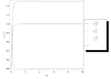
Figure 1: Model I: variation of $x,y,z$ as a function of the $N=\ln(a)$. The initial conditions chosen are $x(0)=0.7,y(0)=0.3,z(0)=0.01$, $\tilde{\omega}=-1.2,\,\,\omega_{r}=\frac{1}{3}$ and $b=0.5$.

The critical points are found for this model by vanishing the first member of (48) and there are the following four points recorded in the below board.

Point	$(x_{c},y_{c},z_{c})$	$\lambda_{1}$	$\lambda_{2}$	$\lambda_{2}$
$P_{11}$	$(0,0,0)$	$3(b-1)$	$-3(b-1)$	$-3(1+2b+\tilde{\omega})$
$P_{12}$	$(0,(1-b),0)$	$-1$	$3(1-b)$	$-3(\tilde{\omega}+3b)$
$P_{13}$	$(0,0,\frac{3}{4}(\frac{4}{3}-b))$	$1$	$4-3b$	$1-3\tilde{\omega}-9b$
$P_{14}$	$(\frac{(1+\tilde{\omega}+2b)}{1+\tilde{\omega}},0,0)$	$3(1+\tilde{\omega}+2b)$	$3(\tilde{\omega}+3b)$	$-1+3(\tilde{\omega}+3b)$

Table 1: Critical points and The eigenvalues for the first model

The point $P_{11}$ is stable when one the following conditions is satisfied

$$\tilde{\omega}<-3,\ \ b<1/18.$$ (49)

$$\tilde{\omega}\geq-3,\ \ \tilde{\omega}<-10/9,\ \ b<1/18.$$ (50)

$$\tilde{\omega}\geq-\frac{10}{9},\ \ \tilde{\omega}<0,\ \ b<-\frac{1}{2}(1+\tilde{\omega}).$$ (51)

$P_{12}$ is an unstable critical point because even if $\lambda_{1}<0$ we have $\lambda_{2}<0$ si $b>1$. $P_{13}$ is stable if $b>1,\tilde{\omega}>-3b$. In parallel $P_{14}$ is not stable because $\lambda_{1}>0$.

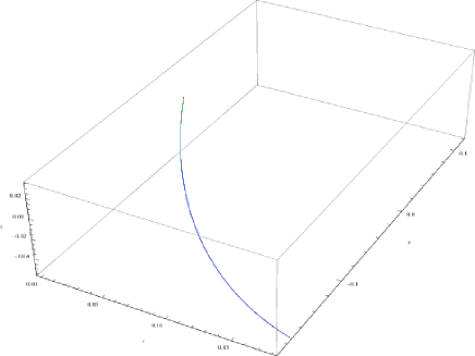
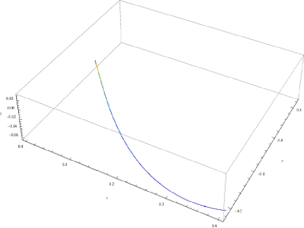
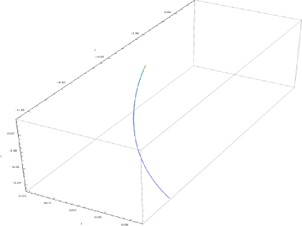
Figure 2: Model I: Phase space for $\tilde{\omega}=(-1,-1.2,-1.5),\,b=0.5,\,\omega_{r}=\frac{1}{3}$

It follows that the matter density dominates for the model I whose parameters stay for the conditions $-1<w_{d}<-\frac{1}{3},w_{u}>0,b=0.5$, $w_{tot}>0$. This conclusion is confirmed by the fig.1 where the matter density dominates whereas the radiation density is above the dark energy density. The fig 2 shows the phase diagram of the interaction between dark energy and the both matter and radiation. According to the model I, the dark energy density behaves like quintessence while matter and radiation densities fall with expansion.

V.2 Interacting model - II

We study another model with the choice of the interaction terms under the following form

$$E_{1}=-3bH\tilde{\rho},\ \ E_{2}=3bH(\tilde{\rho}-\rho_{m}),\ \ E_{3}=3bH\rho_{m}.$$ (52)

This model shows indeed the situation in which the dark energy looses his density in favor of the matter whereas the radiation density increases because of its interaction with the matter.

$$\frac{dx}{dN} = 3x\Big{(}x+y+z+\tilde{\omega}x+\omega_{r}z\Big{)}-3bx-3x(1+\tilde{\omega}),$$ (53)

$$\frac{dy}{dN} = 3y\Big{(}x+y+z+\tilde{\omega}x+\omega_{r}z\Big{)}+3b(x-y)-3y,$$ (54)

$$\frac{dz}{dN} = 3z\Big{(}x+y+z+\tilde{\omega}x+\omega_{r}z\Big{)}+3by-3z(1+\omega_{r}),$$ (55)

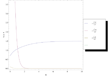
Figure 3: Model I: variation of $x,y,z$ as a function of the $N=\ln(a)$. The initial conditions chosen are $x(0)=0.7,y(0)=0.3,z(0)=0.01$, $\tilde{\omega}=-1.2,\,\,\omega_{r}=\frac{1}{3}$ and $b=0.5$.

We have free critical points

Points	$\lambda_{1}$	$\lambda_{2}$	$\lambda_{3}$	$(x_{c},y_{c},z_{c})$
$P_{21}$	$3(b-1)$	$-3(b-1)$	$-3(1+2b+\tilde{\omega})$	$(0,\quad 0,\quad 0)$
$P_{22}$	$-1$	$3(1-b)$	$-3(\tilde{\omega}+3b)$	$(0,\quad 0,\quad 1)$
$P_{23}$	$1$	$4-3b$	$1-3\tilde{\omega}-9b$	$\Big{(}0,\quad(1-3b),\quad 3b\Big{)}$
$P_{24}$	$3(1+\tilde{\omega}+2b)$	$3(\tilde{\omega}+3b)$	$-1+3(\tilde{\omega}+3b)$	$\Bigg{(}-\,{\frac{3\left(2+\tilde{\omega}\right)\left(b-\tilde{\omega}-1\right)\left(b-\tilde{\omega}-7/3\right)}{3\,{\tilde{\omega}}^{3}+\left(16-3\,b\right){\tilde{\omega}}^{2}+\left(-6\,b+27\right)w_{{d}}+14+{b}^{2}+b}},\newline -\,{\frac{b3\left(b-\tilde{\omega}-7/3\right)\left(b-\tilde{\omega}-1\right)}{3\,{\tilde{\omega}}^{3}+\left(16-3\,b\right){\tilde{\omega}}^{2}+\left(-6\,b+27\right)\tilde{\omega}+14+{b}^{2}+b}},\newline \,{\frac{3\left(b-\tilde{\omega}-1\right){b}^{2}}{14+16\,{\tilde{\omega}}^{2}-6\,\tilde{\omega}b+{b}^{2}-3\,{\tilde{\omega}}^{2}b+3\,{w_{{d}}}^{3}+27\,\tilde{\omega}+b}}\Bigg{)}$

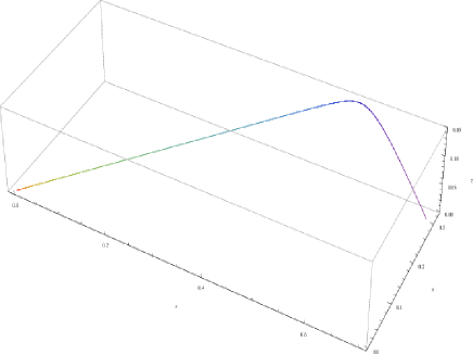
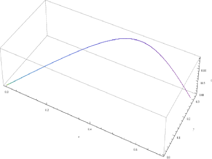
Figure 4: Model II: Phase space for $\tilde{\omega}=(-1,-1.2,-1.5),\,b=0.5,\,\omega_{r}=\frac{1}{3}$

$P_{21}$, $P_{24}$ are conditionally stable if $b>1+\tilde{\omega}$ (for $P_{21}$) and $\tilde{\omega}>-2$ and then

$b<1+\tilde{\omega}$ ( for $P_{24}$ ). But $P_{22}$ and $P_{23}$ are unstable because $\lambda_{1}>0$0.

The figures 3 and 4 show the dynamic of the model II. We notice for this model that there is a great domination of dark energy while the energy densities of the radiation and the matter have declined considerably. This situation is well compatible with the recent observational data which show that the dark energy is the very important responsible of the expansion of Universe. We also point out from these figures that if $N\sim 2$, the radiation declines and goes towards zero. The figure 4 is related to the phase diagram of radiation and dark energy interaction. For the model in study, the behavior of the dark energy is similar to quintessence while the matter and radiation tumble during the expansion.

V.3 Interacting Model - III

Let us take the following interaction terms jamil8

$$E_{1}=-6b\kappa^{2}H^{-1}\tilde{\rho}\rho_{r},\ \ E_{2}=E_{3}=3b\kappa^{2}H^{-1}\tilde{\rho}\rho_{r}.$$ (56)

The system in (44) becomes

$$\frac{dx}{dN} = 3x\Big{(}x+y+z+\tilde{\omega}x+\omega_{r}z\Big{)}-3x-3\tilde{\omega}x-18bxz,$$

$$\frac{dy}{dN} = 3y\Big{(}x+y+z+\tilde{\omega}x+w_{r}z\Big{)}-3y+9bxz,$$ (57)

$$\frac{dz}{dN} = 3z\Big{(}x+y+z+\tilde{\omega}x+\omega_{r}z\Big{)}-3z-3\omega_{r}z+9bxz.$$

.

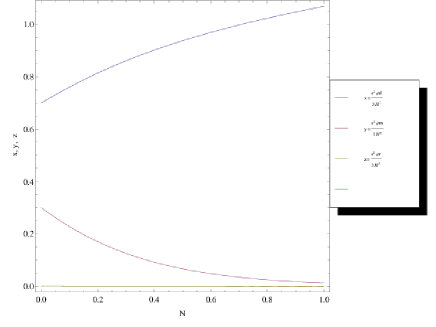
Figure 5: Model III: variation of $x,y,z$ as a function of the $N=\ln(a)$. The initial conditions chosen are $x(0)=0.7,y(0)=0.3,z(0)=0.01$, $\tilde{\omega}=-1.2,\,\,\omega_{r}=\frac{1}{3}$ and $b=0.5$.

Points	$\lambda_{1}$	$\lambda_{2}$	$\lambda_{3}$	$(x_{c},y_{c},z_{c})$
$P_{31}$	$-3$	$-4$	$-3(1+\tilde{\omega})$	$\ (0,\quad 0,\quad 0)$
$P_{32}$	$3$	$-1$	$-3\tilde{\omega}$	$\ (0,\quad 1,\quad 0)$
$P_{33}$	$3\tilde{\omega}$	$3(1+\tilde{\omega})$	$+9\,b-1+3\,\tilde{\omega}$	$\ (0,\quad 0,\quad 1)$
$P_{34}$	$4$	$1-9b$	$-9b+1-3\tilde{\omega}$	$\ (1,\quad 0,\quad 0)$
$P_{35}$	-	-	-
$P_{35}$	-	-	-	$\Bigg{(}{\frac{\left(\tilde{\omega}+6\,b-\frac{1}{3}\right)}{b\left(+6\,b-\frac{1}{3}+2\,\tilde{\omega}\right)}},\newline {\frac{\,-3\,b+18\,{b}^{2}+{\tilde{\omega}}^{2}-2\,\tilde{\omega}\frac{1}{3}+9\,\tilde{\omega}b+\frac{1}{9}}{3b\left(6\,b-\frac{1}{3}+2\,\tilde{\omega}\right)}},\newline -\,{\frac{\tilde{\omega}\left(+3\,b-\frac{1}{3}+\tilde{\omega}\right)}{3b\left(6\,b-\frac{1}{3}+2\,\tilde{\omega}\right)}}\Bigg{)}$

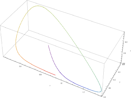
Figure 6: Model III: Phase space for $\tilde{\omega}=(-1,-1.2,-1.5),\,b=0.5,\,\omega_{r}=\frac{1}{3}$

$P_{31}$ is stable for $w_{d}>-1$. $P_{32}$ , $P_{34}$ are unstable. $P_{33}$ is systematically stable when $w_{d}<-1$, $b<\frac{1-3w_{d}}{9(1+\alpha)}$.

We present here the dynamic of model III through the figures 5 and 6. Here we note a gradual increase for the dark energy whereas the energy densities of the radiation and the matter are tending to zero. These facts are compatible with the recent observational data showing that Universe is accelerated expansion because of the strong presence of dark energy in Universe. This analysis shows also that becomes nonexistent because of the strong domination of dark energy. The phase diagram of interaction between dark energy and the both matter and radiation is plotted in figure 6. In parallel with the previous models, this model is also one of those where the behavior the energy density of dark energy is that of quintessence while the densities of radiation and matter are going to vanish during the the expansion.

V.4 Interacting Model - IV

Let’s search for new model generalized by the new following interaction terms:

$$E_{1} = -3b\kappa^{2}H^{-1}\tilde{\rho}\rho_{r},$$

$$E_{2} = 3b\kappa^{2}H^{-1}(\tilde{\rho}\rho_{r}-\rho_{m}\rho_{r}),$$

$$E_{3} = 3b\kappa^{2}H^{-1}\rho_{m}\rho_{r}.$$ (58)

The system in (44) takes the form

$$\frac{dx}{dN} = 3x\Big{(}x+y+z+\tilde{\omega}x+\omega_{r}z\Big{)}-3x-3\tilde{\omega}x-9bxz,$$

$$\frac{dy}{dN} = 3y\Big{(}x+y+z+\tilde{\omega}x+\omega_{r}z\Big{)}-3y+9b(xz-yz),$$ (59)

$$\frac{dz}{dN} = 3z\Big{(}x+y+z+\tilde{\omega}x+\omega_{r}z\Big{)}-3z-3\omega_{r}z+9byz.$$

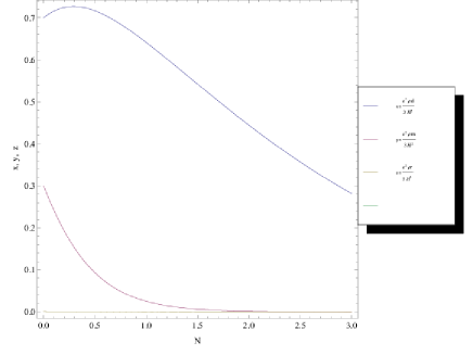
Figure 7: Model IV: variation of $x,y,z$ as a function of the $N=\ln(a)$. The initial conditions chosen are $x(0)=0.7,y(0)=0.3,z(0)=0.01$, $\tilde{\omega}=-1.2,\,\,\omega_{r}=\frac{1}{3}$ and $b=0.5$.

One obtains seven critical points

Points	$\lambda_{1}$	$\lambda_{2}$	$\lambda_{3}$	$(x_{c},y_{c},z_{c})$
$P_{41}$	$-3$	$-4$	$-3(1+\tilde{\omega})$	$\ (0,\quad 0,\quad 0)$
$P_{42}$	$3$	$-1$	$-3\tilde{\omega}$	$\ (1,\quad 0,\quad 0)$
$P_{43}$	$3\tilde{\omega}$	$3\tilde{\omega}-1$	$3\tilde{\omega}-1$	$\ (0,\quad 1,\quad 0)$
$P_{44}$	$3(1+\tilde{\omega})$	$-9b+1$	$-3\tilde{\omega}-9b+1$	$\ (0,\quad 0,\quad 1)$
$P_{45}$	-	-	-	$\ \Big{(}\frac{1}{3}\frac{\frac{4}{3}\tilde{\omega}}{b(1+\tilde{\omega})},\frac{4}{9b},-\frac{1}{3}\frac{1+\tilde{\omega}}{b}\Big{)}$
$P_{46}$	-	-	-	$\Big{(}\,{\frac{\tilde{\omega}+3\,b+3\,-1/3}{3b}},\newline -\,{\frac{\left(-\frac{1}{3}+\tilde{\omega}\right)\left(\tilde{\omega}+3\,b+-\frac{1}{3}\right)}{3b\left(3\,b-\frac{1}{3}\right)}},\newline {\frac{\tilde{\omega}\left(-\frac{1}{3}+\tilde{\omega}\right)}{3b\left(3\,b-\frac{1}{3}\right)}}\Big{)}$
$P_{4}7$	$-3\tilde{\omega}$	$\frac{\sqrt{3}\sqrt{b\left(-4/9+3\,b+\,b\right)}}{b}$	$-{\frac{\sqrt{3}\sqrt{b\left(-4/9+3\,b+\,b\right)}}{b}}$	$\ (0,\frac{4}{9b},-\frac{1}{3b})$

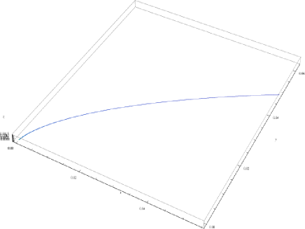
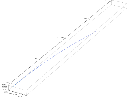
Figure 8: Model IV: Phase space for $\tilde{\omega}=(-1,-1.2,-1.5),\,b=0.5,\,\omega_{r}=\frac{1}{3}$

We remark for this model that $P_{41}$ is stable for $\tilde{\omega}>-1$ , $P_{42}$ is also stable for $\tilde{\omega}<-1$ while $P_{43}$ and $P_{47}$ are unstable. $P_{44}$ is stable for $\tilde{\omega}<-1$ and $b>\frac{1}{9}$. It is also possible to determine the stability of point $P_{45}$. The stabilities of the point $P_{47}$ and also $P_{35}$ from the model III are not easy to be studied because the matrix of Jacobi in these cases is not diagonal and the behaviors of its eigenvalues are not trivial. This means that we can not theoretically know if these points are stable or not. Consequently these cases are analytically and numerically impossible to be studied. Therefore, the dynamic behaviors of the model IV behavior have been plotted in the figures 7 and 8 which show that the density of the dark energy quickly rise up to $N\sim 0,5$ and after decreases sharply (same behavior with quintessence) whereas the energy densities of radiation and matter decrease and tend to zero when $N\sim 1,8$.

VI Stability of $T+\mathcal{T}^{\mathcal{N}}$ model

This section is devoted to the study of the stability of model $f(T,\mathcal{T})=T+\mathcal{T}^{\mathcal{N}}$ by using the power-law and the de Sitter solutions.

We are interested here to the perturbation of both geometric parts and matter of the generalized equations of motion. To do so, we have focused our attention on the Hubble parameter for geometric perturbation and energy density for ordinary primordial matter perturbation and we have followed the same way as it is done in antoniode ; diegoalvaro .

$$H(t)=H_{b}(t)(1+\delta(t)),\quad\rho(t)=\rho_{b}(t)(1+\delta_{m}(t)).$$ (60)

$H_{b}(t)$ and $\rho_{b}(t)$ denote the Hubble parameter and the energy density of the ordinary matter of the background respectively. Taking into consideration the interaction term, the continuity equation of the ordinary matter becomes the following differential equation

$$\dot{\rho_{b}}(t)+3H_{b}(t)\rho_{b}(t)(1+\omega+q)=0\,,$$ (61)

whose resolution leads to:

$$\rho_{b}(t)=\rho_{0}\ e^{-3(1+\omega+q)\int{H_{b}(t)}dt},$$ (62)

where $\rho_{0}$ is an integration constant. In order to study the linear perturbation about $H(t)$ and $\rho(t)$, we develop $\mathcal{T}^{\mathcal{N}}$ in a series of $\mathcal{T}_{b}=\rho_{b}(1-3\omega)$ as:

$$f(\mathcal{T})=f^{b}+f_{\mathcal{T}}^{b}(\mathcal{T}-\mathcal{T}_{b})+O^{2},$$ (63)

The function $\mathcal{T}^{\mathcal{N}}$ and its derivatives are computed at $\mathcal{T}=\mathcal{T}_{h}$. According to the Einstein-Hilbert term, the strangeness here is the effect coming from $\mathcal{T}^{\mathcal{N}}$. By putting (60) into (63) in the the first generalized Friedmann equation; one gets

$$3H^{2}=\rho-\frac{1}{2}\left(f+12H^{2}f_{T}\right)+3f_{\mathcal{T}}\left(\frac{\rho+p}{3}\right),$$ (64)

which gives after simplification

$$6H_{b}^{2}(t)\delta(t)=\big{[}\rho_{b}+\rho_{b}f_{\mathcal{T}}^{b}(\frac{3-\omega}{2})+\rho_{b}^{2}(1-2\omega-3\omega^{2})f_{\mathcal{T}\mathcal{T}}^{b}\big{]}\delta_{m}(t).$$ (65)

Considering that the ordinary matter is essentially the dust, we obtain the simple expression

$$6H_{b}^{2}(t)\delta(t)=\big{[}\rho_{b}+3\rho_{b}f_{\mathcal{T}}^{b}+2\rho_{b}^{2}f_{\mathcal{T}\mathcal{T}}^{b}\big{]}\delta_{m}(t),.$$ (66)

For matter pertubation function, we have the following differential equation

$$\dot{\delta_{m}}(t)+3(1+\omega+q)H_{b}(t)\delta(t)=0.$$ (67)

Eliminating $\delta(t)$ between (65) and (67), we obtain also the differential equation

$$2H_{b}\dot{\delta}_{m}(t)+(1+\omega+q)\big{[}\rho_{b}+\rho_{b}f_{\mathcal{T}}^{b}\left(\frac{3-\omega}{2}\right)+\rho_{b}^{2}(1-2\omega-3\omega^{2})f_{\mathcal{T}\mathcal{T}}^{b}\big{]}\delta_{m}(t)=0.$$ (68)

The direct resolution of this differential equation gives

$$\delta_{m}(t)=C_{0}\exp\left\{-\left(\frac{1+\omega+q}{2}\right)\int\frac{\rho_{b}}{H_{b}}\left[1+f_{\mathcal{T}}^{b}\left(\frac{3-\omega}{2}\right)+\rho_{b}(1-2\omega-3\omega^{2})f_{\mathcal{T}\mathcal{T}}^{b}\right]dt\right\},$$ (69)

where $C_{0}$ is an integration constant. From Eq. (67) one can extract

$$\delta(t)=\frac{C_{0}C_{\mathcal{T}}}{6H_{b}}\exp\left\{-\left(\frac{1+\omega+q}{2}\right)\int C_{\mathcal{T}}dt\right\},$$ (70)

with

$$C_{\mathcal{T}}=\frac{\rho_{b}}{H_{b}}\left[1+f_{\mathcal{T}}^{b}\left(\frac{3-\omega}{2}\right)+\rho_{b}\left(1-2\omega-3\omega^{2}\right)f_{\mathcal{T}\mathcal{T}}^{b}\right].$$ (71)

VI.1 Stability of de Sitter solutions

In this case, the Hubble parameter is written as

$$H_{b}(t)=H_{0}\rightarrow a(t)=a_{0}e^{H_{0}t}.$$ (72)

The expression (62) becomes,

$$\rho_{b}(t)=\rho_{0}e^{-3(1+\omega+q)H_{0}t}.$$ (73)

From relation $d{\rho_{b}}=-3(1+\omega+q)H_{0}\rho_{b}dt$ and within an elementary transformation, we get

$$\int C_{\mathcal{T}}dt = -\frac{1}{3H_{0}(1+\omega+q)}\int\frac{1}{\rho_{b}}C_{\mathcal{T}}d{\rho_{b}}$$ (74)

$$= -\frac{1}{3H_{0}^{2}(1+q+\omega)}\Bigg{\{}\rho_{b}+Q\;\frac{(3-\omega)}{2}\rho_{b}^{\mathcal{N}}(1-3\omega)^{\mathcal{N}-1}$$

$$+ Q\;(1-2\omega-3\omega^{2})(\mathcal{N}-1)(1-3\omega)^{\mathcal{N}-2}\rho_{b}^{\mathcal{N}}\Bigg{\}}.$$

By replacing this expression in 69, we obtains

$$\delta_{m}(t)=C_{0}\exp\left\{\frac{1}{6H_{0}^{2}}\left[\rho_{b}+Q\;\frac{(3-\omega)}{2}\rho_{b}^{\mathcal{N}}(1-3\omega)^{\mathcal{N}-1}+Q\;(1-2\omega-3\omega^{2})(\mathcal{\mathcal{N}}-1)(1-3\omega)^{\mathcal{N}-2}\rho_{b}^{\mathcal{N}}\right]\right\}.$$ (75)

Therefore the perturbation function about the geometry can be obtained and given by

$$\delta(t) = \frac{C_{0}C_{\mathcal{T}}}{6H_{0}}\exp\left\{\frac{1}{6H_{0}^{2}}\left[\rho_{b}+Q\;\frac{(3-\omega)}{2}\rho_{b}^{\mathcal{N}}(1-3\omega)^{\mathcal{N}-1}+Q\;(1-2\omega-3\omega^{2})(\mathcal{N}-1)(1-3\omega)^{\mathcal{N}-2}\rho_{b}^{\mathcal{N}}\right]\right\},$$ (76)

with

$$C_{\mathcal{T}}=\frac{1}{H_{0}}\left\{\rho_{b}+Q\;\mathcal{N}\frac{(3-\omega)}{2}\rho_{b}^{\mathcal{N}}(1-3\omega)^{\mathcal{N}-1}+Q\;\mathcal{N}(\mathcal{N}-1)(1-2\omega-3\omega^{2})(1-3\omega)^{\mathcal{N}-2}\rho_{b}^{\mathcal{N}}\right\}$$ (77)

and

$$f(\mathcal{T})=Q\;\mathcal{T}^{\mathcal{N}}.$$ (78)

with $Q$ the one defined in (28) and $\mathcal{N}=-(1-3\omega)/((1+\omega))$. For some suitable values of the input parameters consistent with cosmological observational data, we plot the curve characterizing the behavior of the perturbation function at the left side in Fig 2. We see that as the universe expands, i.e., increasing $Z$, the matter and geometric perturbations functions, $\delta_{m}$ and $\delta$ respectively, goes towards positive values more less than $0.1$ when the time evolves.

VI.2 Stability of Power-Law solutions

Here, the scale factor is written as

$$a(t)\propto t^{n}\quad\rightarrow H_{b}(t)=\frac{n}{t}\,,$$ (79)

and the ordinary energy density (62) becomes

$$\rho_{b}=\rho_{0}t^{-3n(1+\omega+q)}$$ (80)

By making the substitution of $\rho_{b}$ in (68), one gets after resolution, the following expression

$$\delta_{m}(t)=C_{1}\exp\left\{-A\left(\frac{A_{1}}{2+B}t^{2+B}+\frac{A_{2}}{2+\mathcal{N}B}t^{2+\mathcal{N}B}\right)\right\},$$ (81)

with $C_{1}$ an integration constant, and

$$A=\frac{(1+\omega+q)}{2n},\quad A_{1}=\rho_{0},\quad B=-3n(1+\omega+q)$$

$$A_{2}=Q\;\mathcal{N}\rho_{0}^{\mathcal{N}}\left\{\frac{(18\omega^{3}+9\omega^{2}-14\omega+3)}{2(1-3\omega)^{2-\mathcal{N}}}+\frac{\mathcal{N}}{{(1-3\omega)}^{(1-\mathcal{N})}}\right\}.$$ (82)

The use of the relation (67 leads to

$$\delta(t)=\frac{C_{1}}{6n^{2}}\left(A_{1}t^{2+\mathcal{N}}+A_{2}t^{2+B\mathcal{N}}\right)\exp\left\{-A\left(\frac{A_{1}}{2+B}t^{2+B}+\frac{A_{2}}{2+\mathcal{N}B}t^{2+\mathcal{N}B}\right)\right\}.$$ (83)

As we have done in the previous section, we present here the evolution of the perturbation functions in Fig 9 for suitable values of input parameters.

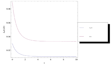
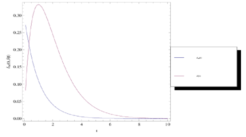
Figure 9: The graph at the left side of the figure presents the evolution of the perturbation functions $\delta_{m}$ and $\delta$ within the de Sitter solutions, while the one at the right side shows the evolution of the perturbation functions within the power-law solutions. The graph are plotted for $n=2/3$, $\Lambda=1.7\times 10^{-121}$, $\rho_{0}=0.1\times 10^{-121}$, $\omega=0$ and $C_{1}=1$ .

VII Conclusion

We undertook in this work cosmological analysis about a model in the framework of the so-called $f(T,\mathcal{T})$ theory. In order to obtain a viable $f(T,\mathcal{T})$ model, we first impose the covariant conservation of the energy-momentum, from which, we get a model of the type $T+f(\mathcal{T})$, being a sort of trace depending function correction to the TT. The obtained model includes parameters depending on the cosmological constant $\Lambda$ and the parameter $\omega$ of the ordinary equation of state. These parameters play a main role in the whole study developed in this manuscript. By the way, we study the dynamics of the cosmological system, analyzing the stability about the critical points. We solve the equations and it appears that for some specific expressions of the interaction term one can obtain attractor solutions. We numerically integrate the equations and show that the evolution of the dark energy density mimics three diffract behaviors: phantom, quintessence and cosmological constant in some interactive forms. We argue that this interaction is purely phenomenological and is consistent with the observational data. Our result shows that for both de Sitter and power-law solutions, the perturbations functions converge traducing the stability of the model.

Moreover, the stability of the model is checked within the de Sitter and power-law solutions by performing linear perturbation about the physical critical points. We see that for the both considered solutions, the model presents stability through the convergence of the geometric and matter perturbation functions $\delta$ and $\delta_{m}$.

References

- (1) C. W. Misner, K. S. Thorne, and J. H. Wheeler, Gravitation, W. H. Freeman and Company, 1973.
- (2) Szekeres P: The Gravitational Compass, J. Maths. Phys. 6 (1965), 1387.
- (3) J. L. Synge. On the Deviation of Geodesics and Null Geodesics, Particularly in Relation to the Properties of Spaces of Constant Curvature and Indefinite Line Element. Ann. Math. 35:705 (1934).
- (4) F. A. E. Pirani. On the Physical Significance of the Riemann Tensor. Acta Phys. Polon. 15:389 (1956).
- (5) G. F. R. Ellis and H. Van Elst. Deviation of geodesics in FLRW spacetime geometries (1997). Preprint in [arXiv:gr-qc/9709060v1].
- (6) S.L. Shapiro and S.A. Teukolsky, Black Holes, White Dwarfs and Neutron Satrs (Wile-Interscience, New York 1983).
- (7) K.S. Thorne, in S. Hawking and W. Israel, eds, 300 Year of Gravitation (Cambridge University, Cambridge 1987) p. 330.
- (8) Raychaudhuri A K: Relativistic Cosmology, Phys. Rev. 98 (1955), 1123.
- (9) Mattig W: Uber den Zusammenhang zwischen Rotverschiebung und scheinbarer Helligkeit, Astr. Nach. 284 (1958), 109.
- (10) Pirani F A E: On the Physical Significance of the Riemann Tensor, Acta Phys. Polon. 15 (1956),389.
- (11) D. N. Spergel, et. al., Astrophys. J. Suppl. 170, (2007) 377, arXiv:astro-ph/0603449.
- (12) J. K. Adelman-McCarthy, et. al., Astrophys. J. Suppl. 175, (2008) 297, arXiv:0707.3413[astro-ph].
-
(13)
R.Aldrovandi and J.G.Pereira,TELEPARALLEL GRAVITY,
in http://www.ift.unesp.br/users/jpereira/tele.pdf. - (14) A. De Felice and S. Tsujikawa, Living Rel. Rev. 13, 3 (2010) [arXiv:1002.4928 [gr-qc]]; K. Bamba, S. Capozziello, S. Nojiri, S. D. Odintsov. Astrophys. Space Sci. 342, 155 (2012) [arXiv:1205.3421 [gr-qc]]; S. Nojiri and S. D. Odintsov, ECONF C 0602061, 06 (2006); Int. J. Geom. Meth. Mod. Phys. 4, 115-146 (2007) [arXiv:hep-th/0601213]; Phys. Rept. 505, 59-144 (2011) [arXiv:1011.0544].
- (15) T. Harko, F. S. N. Lobo, S. Nojiri and S. D. Odintsov, ?f(R, T ) gravity,? Phys. Rev. D 84 (2011) 024020. [arXiv:1104.2669 [gr-qc]].
- (16) M. J. S. Houndjo, Int. J. Mod. Phys. D. 21, 1250003 (2012). arXiv: 1107.3887 [astro-ph.CO].
- (17) M. J. S. Houndjo and O. F. Piattella, Int. J. Mod. Phys. D. 21, 1250024 (2012). arXiv: 1111.4275 [gr.qc].
- (18) D. Momeni, M. Jamil and R. Myrzakulov, Euro. Phys. J. C 72, arXiv: 1107.5807[physics.gen-ph].
- (19) M. J. S. Houndjo, C. E. M. Batista, J. P. Campos and O. F. Piattella,?? [arXiv:1203.6084 [gr-qc]].
- (20) F. G. Alvarenga, M. J. S. Houndjo, A. V. Monwanou and Jean. B. Chabi-Orou,?? arXiv: 1205.4678 [gr-qc].
- (21) S. ’i. Nojiri and S. D. Odintsov, “Modified Gauss-Bonnet theory as gravitational alternative for dark energy,” Phys. Lett. B 631, 1 (2005) [hep-th/0508049]; S. Nojiri, S. D. Odintsov, A. Toporensky, P. Tretyakov, arXiv:0912.2488.
- (22) K. Bamba, S. D. Odintsov, L. Sebastiani, S. Zerbini, arXiv:0911.4390.
- (23) K. Bamba, C.-Q. Geng, S. Nojiri, S. D. Odintsov, arXiv:0909.4397.
- (24) M.E. Rodrigues, M.J.S. Houndjo, D. Momeni, R. Myrzakulov, arXiv:1212.4488.
- (25) M. J. S. Houndjo, M. E. Rodrigues, D. Momeni, R. Myrzakulov . arXiv:1301.4642 [gr-qc].
- (26) J. Amorós, J. de Haro and S. D. Odintsov, “Bouncing Loop Quantum Cosmology from gravity,” Physical Review D 87, 104037 (2013) [arXiv:1305.2344 [gr-qc]]; K. Bamba, J. de Haro and S. D. Odintsov, “Future Singularities and Teleparallelism in Loop Quantum Cosmology,” JCAP 1302 (2013) 008 [arXiv:1211.2968 [gr-qc]]; K. Bamba, S. ’i. Nojiri and S. D. Odintsov, “Effective gravity from the higher-dimensional Kaluza-Klein and Randall-Sundrum theories,” arXiv:1304.6191 [gr-qc]; G. R. Bengochea, R. Ferraro and , Phys. Rev. D 79, 124019 (2009) [arXiv:0812.1205 [astro-ph]].
- (27) E. V. Linder, Phys.Rev. D 81, 127301 (2010) [Erratum-ibid. D 82, 109902 (2010)] [arXiv:1005.3039 [astro-ph.CO]].
- (28) M. Jamil, D. Momeni and R. Myrzakulov, Eur. Phys. J. C 72 (2012) 2267 [arXiv:1212.6017 [gr-qc]].
- (29) R. Myrzakulov, Entropy 14 (2012) 1627[arXiv:1212.2155 [gr-qc]].
- (30) M. R. Setare and N. Mohammadipour, JCAP 1211 (2012) 030 [arXiv:1211.1375 [gr-qc]].
- (31) M.R. Setare, N. Mohammadipour, JCAP 01 (2013) 015 [arXiv: 1301.4891].
- (32) M. Jamil, D. Momeni, R. Myrzakulov and P. Rudra, J. Phys. Soc. Jap. 81 (2012) 114004 [arXiv:1211.0018 [physics.gen-ph]].
- (33) M. E. Rodrigues, M. J. S. Houndjo, D. Saez-Gomez and F. Rahaman, Phys. Rev. D 86 (2012) 104059 [arXiv:1209.4859 [gr-qc]].
- (34) M. Jamil, D. Momeni and R. Myrzakulov, Eur. Phys. J. C 72 (2012) 2122 [arXiv:1209.1298 [gr-qc]].
- (35) R. Myrzakulov, Eur. Phys. J. C 72 (2012)2203 [arXiv:1207.1039 [gr-qc]].
- (36) M. J. S. Houndjo, D. Momeni and R. Myrzakulov, Int. J. Mod. Phys. D 21 (2012) 1250093 [arXiv:1206.3938 [physics.gen-ph]].
- (37) M. E. Rodrigues, M. H. Daouda and M. J. S. Houndjo, arXiv:1205.0565 [gr-qc].
- (38) M. R. Setare and M. J. S. Houndjo, arXiv:1203.1315 [gr-qc].
- (39) K. Bamba, M. Jamil, D. Momeni and R. Myrzakulov, arXiv:1202.6114 [physics.gen-ph].
- (40) K. Bamba, R. Myrzakulov, S. ’i. Nojiri and S. D. Odintsov, Phys. Rev. D 85 (2012)104036 [arXiv:1202.4057 [gr-qc]].
- (41) M. Jamil, D. Momeni and R. Myrzakulov, Eur. Phys. J. C 72 (2012) 2267 [arXiv:1212.6017[gr-qc]].
- (42) M. Jamil, D. Momeni and R. Myrzakulov, Gen. Rel. Grav. 45 (2013) 263 [arXiv:1211.3740 [physics.gen-ph]].
- (43) M. Jamil, D. Momeni and R. Myrzakulov, Eur. Phys. J. C 72 (2012) 2122 [arXiv:1209.1298 [gr-qc]].
- (44) M. Jamil, D. Momeni and R. Myrzakulov, Eur. Phys. J. C 72 (2012) 2075 [arXiv:1208.0025 [gr-qc]].
- (45) M. Jamil, K. Yesmakhanova, D. Momeni and R. Myrzakulov, Central Eur. J. Phys. 10 (2012) 1065 [arXiv:1207.2735 [gr-qc]].
- (46) M. J. S. Houndjo, D. Momeni and R. Myrzakulov, Int. J. Mod. Phys. D 21 (2012) 1250093 [arXiv:1206.3938 [physics.gen-ph]].
- (47) M. Jamil, D. Momeni and R. Myrzakulov, Eur. Phys. J. C 72 (2012) 1959 [arXiv:1202.4926 [physics.gen-ph]].
- (48) M. H. Daouda, M. E. Rodrigues and M. J. S. Houndjo, Phys. Lett. B 715 (2012) 241 [arXiv:1202.1147 [gr-qc]].
- (49) M. Jamil, S. Ali, D. Momeni, R. Myrzakulov and Eur. Phys. J. C 72, 1998 (2012) [arXiv:1201.0895 [physics.gen-ph]].
- (50) M. Jamil, D. Momeni, N. S. Serikbayev, R. Myrzakulov and , Astrophys. Space Sci. 339, 37 (2012) [arXiv:1112.4472 [physics.gen-ph]].
- (51) M. Jamil, D. Momeni, M. A. Rashid and , Eur. Phys. J. C 71, 1711 (2011) [arXiv:1107.1558 [physics.gen-ph]].
- (52) M. Hamani Daouda, M. E. Rodrigues and M. J. S. Houndjo, Eur. Phys. J. C 72 (2012) 1893 [arXiv:1111.6575 [gr-qc]].
- (53) M. Hamani Daouda, M. E. Rodrigues and M. J. S. Houndjo, Eur. Phys. J. C 72 (2012) 1890 [arXiv:1109.0528 [physics.gen-ph]].
- (54) R. Myrzakulov, Gen. Rel. Grav. 44 (2012) 3059 [arXiv:1008.4486 [physics.gen-ph]].
- (55) K. K. Yerzhanov, S. .R. Myrzakul, I. I. Kulnazarov and R. Myrzakulov, arXiv:1006.3879 [gr-qc].
- (56) R. Myrzakulov, Eur. Phys. J. C 71 (2011) 1752 [arXiv:1006.1120 [gr-qc]].
- (57) M. E. Rodrigues, M. J. S. Houndjo, D. Momeni, R. Myrzakulov and , arXiv:1302.4372 [physics.gen-ph].
- (58) J. M. Bardeen, B. Carter, S. W. Hawking , Commun. Math. Phys. 31 (1973) 161-170.
- (59) N. Tamanini and C. G. Boehmer, Phys. Rev. D 86, 044009 (2012), arXiv:1204.4593 [gr-qc].
- (60) Baojiu Li, T. P. Sotiriou and J. D. Barrow, Phys. Rev. D 83, 064035 (2011); Phys. Rev. D 83, 104030 (2011).
- (61) M. J. S. Houndjo, D. Momeni, R. Myrzakulov and M. E. Rodrigues,arXiv:1304.1147.
- (62) C. Deliduman and B. Yapiskan, arXiv:1103.2225v3 [gr-qc].
- (63) M. Hamani Daouda, M. E. Rodrigues and M. J. S. Houndjo, Eur. Phys. J. C 71 (2011) 1817 [arXiv:1108.2920 [astro-ph.CO]].
- (64) I.G.Salako, M.E.Rodrigues, A.V.Kpadonou, M. J.S.Houndjo and J.Tossa JCAP 060, 1475-7516 (2013)
- (65) M. E. Rodrigues, I. G. Salako, M. J. S. Houndjo, J. Tossa Int. J. Mod. Phys. D 23, 1450004 (2014)
- (66) Davood Momeni, Ratbay Myrzakulov.: arXiv:1405.5863 [gr-qc]
- (67) Tiberiu Harko, Francisco S. N. Lobo, G. Otalora,and Emmanuel N. Saridakis http://arxiv.org/abs/1405.0519v1
- (68) Ines G. Salako, Abdul Jawad, Surajit Chattopadhyay,
- (69) S. B. Nassur, M. J. S. Houndjo, A. V. Kpadonou, M. E. Rodrigues, J. Tossa, http://arxiv.org/abs/1506.09161
- (70) F. G. Alvarenga, A. de la Cruz-Dombriz, M. J. S. Houndjo, M. E. Rodrigues, D. Sáez-Gómez, Phys. Rev. D 87, 103526 (2013). arXiv:1302.1866 [gr-qc].
- (71) M. Jamil, D. Momeni, M. A. Rashid, Eur. Phys. J. C 71, 1711 (2011); S. Chen, J. Jing, Class. Quan. Grav. 26, 155006 (2009).
- (72) A. De Felice and S. Tsujikawa, Phys. Lett. B 675, 1-8 (2009); arXiv: 0810.5712 [hep-th].
- (73) A. de la Cruz-Dombriz and D. Sáez-Gómez, Class. Quantum Grav 29, 245014 (2012), arXiv: 1112.4481 [gr-qc].