Counterpart of the Darrieus-Landau instability at a magnetic deflagration front

Abstract

The magnetic instability at the front of the spin avalanche in a crystal of molecular magnets is considered. This phenomenon reveals similar features with the Darrieus-Landau instability, inherent to classical combustion flame fronts. The instability growth rate and the cut-off wavelength are investigated with respect to the strength of the external magnetic field, both analytically in the limit of an infinitely thin front and numerically for finite-width fronts. The presence of quantum tunneling resonances is shown to increase the growth rate significantly, which may lead to a possible transition from deflagration to detonation regimes. Different orientations of the crystal easy axis are shown to exhibit opposite stability properties. In addition, we suggest experimental conditions that could evidence the instability and its influence on the magnetic deflagration velocity.

I Introduction

The Darrieus-Landau instability, first described in the context of combustion, is a hydrodynamic instability that is caused by the thermal expansion of the burning gas Landau and Lifshitz (1989); Bychkov and Liberman (2000); Matalon (2007). It is characterized by the fact that the growth rate of the instability at the flame front is positive for perturbations of any wavelength, and is responsible for the curving of initially planar flames. In addition to combustion, the Darrieus-Landau instability has been observed in different types of plasmas, from the interstellar medium to inertial confinement fusion, see, e.g., Refs. Clavin and Masse (2004); Sanz, Masse, and Clavin (2006); Gamezo, Khokhlov, and Oran (2005); Inoue, Inutsuka, and Koyama (2006); Bychkov et al. (2007); Bychkov, Modestov, and Marklund (2008); Bychkov et al. (2011).

Another system in which combustion-like processes have been observed are crystals of molecular (nano) magnets. These molecular magnets have large spin ($S\sim 10$), and their crystals present an anisotropy, with an “easy” axis along which the spin will align. In the presence of an external magnetic field along the easy axis, the two different orientations will not have the same energy, resulting in an effective skewed double-well potential (see Gatteschi and Sessoli (2003) and references therein). A crystal prepared in the metastable magnetic orientation, after local heating to overcome the activation energy, will see a propagation of the spin reversal, as the energy released by the spin flip will propagate to neighboring molecules, in a process dubbed a spin avalanche or magnetic deflagration Suzuki et al. (2005); Hernández-Mínguez et al. (2005); Garanin and Chudnovsky (2007); Villuendas et al. (2008); Decelle et al. (2009). The spin reversal can also occur without the activation energy being attained, through spin tunneling Chudnovsky and Tejada (1998); del Barco et al. (2005). This phenomenon leads to the presence, for certain values of the magnetic field strength, of tunneling resonances that greatly increase the speed of propagation of the spin reversal front Hernández-Mínguez et al. (2005); Garanin and Chudnovsky (2007); McHugh et al. (2007); Macià et al. (2009); Vélez et al. (2014).

In previous work Jukimenko et al. (2014), we demonstrated that the propagation of this magnetic deflagration front is unstable, due to the fact that any distortion in the front increases the local magnetic field, creating a positive feedback. In this paper, we take a closer look at the stability of the front, and derive an analytical expression for the instability growth rate, in the limit of an infinitely thin front. We also study the instability numerically, accounting for a finite magnetic front thickness. Our results are also compared to experimental data Hernández-Mínguez et al. (2005), taking into account the presence of tunneling resonances.

II Deflagration in crystals of molecular nanomagnets

We consider a crystal of Mn₁₂-acetate, which has an effective spin number $S=10$ Caneschi et al. (1991), placed in an external magnetic field $B_{z}$ aligned along the $z$-axis, which corresponds also to the easy axis. The energy levels of molecular magnet can be described by the simplified spin Hamiltonian Garanin and Chudnovsky (2007)

$$\hat{\mathcal{H}}=-D\hat{S}_{z}^{2}-g\mu_{B}B_{z}\hat{S}_{z},$$ (1)

where $D=0.65\ \mathrm{K}$ del Barco et al. (2005), $g=1.93$ is the gyromagnetic factor Sessoli et al. (1993), and $\mu_{B}$ is the Bohr magneton. The first term is due to the anisotropy of the crystal, while the second term describes the dipole interaction between the external magnetic field and the spin of the molecule. We consider a crystal with all molecules initially in the $S_{z}=-10$ metastable state, which is then locally heated at one extremity, and study the propagation of the spin reversal to the stable $S_{z}=10$ state. Using Hamiltonian (1), we find the Zeeman energy release $Q$

$$Q=2g\mu_{B}B_{z}S,$$ (2)

and the energy barrier or activation energy $E_{a}$,

$$E_{a}=DS^{2}-g\mu_{B}B_{z}S+\frac{g^{2}}{4D}\mu_{B}^{2}B_{z}^{2},$$ (3)

expressed in temperature units per molecule. For the particular external field $B_{z}=$0.5\text{\,}\mathrm{T}$$, these quantities are depicted in Fig. 1 together with the energy levels of Mn₁₂-acetate.

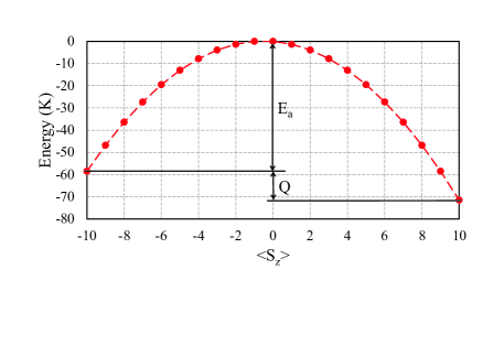
Figure 1: (Color online) Energy levels of a molecular magnet Mn₁₂-acetate in an external magnetic field $B_{z}=$0.5\text{\,}\mathrm{T}$$. A molecule initially in the metastable state $S_{z}=-10$ (on the left) must overcome an energy threshold $E_{a}$ in order to relax to the stable state $S_{z}=10$ (on the right). After relaxation, the energy difference (Zeeman energy) $Q$ is released as heat.

The evolution of the system is governed by the heat transfer and the dynamics of the molecules in the metastable state. The Zeeman energy release is transformed into phonon thermal energy and is described as

$$\frac{\partial E}{\partial t}=\nabla\cdot(\kappa\nabla E)-Q\frac{\partial n}{\partial t},$$ (4)

where $E$ is the phonon energy and $\kappa$ is the thermal diffusion constant, which depends on temperature as $\kappa=\kappa_{0}T^{-\beta}$. The number of molecules in the metastable state evolves according to

$$\frac{\partial n}{\partial t}=-\Gamma\left(n-n_{\mathrm{eq}}\right),$$ (5)

where $n_{\mathrm{eq}}=\left[1+\exp\left(Q/T\right)\right]^{-1}$ is the thermal equilibrium concentration Modestov, Bychkov, and Marklund (2011a). The prefactor in Eq. (5) stands for the thermal relaxation rate over the potential barrier $E_{a}$, shown Fig. 1. In the simplest form, it may be written as the Arrhenius law

$$\Gamma=\Gamma_{R}\exp\left(-E_{a}/T\right).$$ (6)

Generally speaking, the $\Gamma_{R}$ factor is not a constant, but depends on both longitudinal and perpendicular components of the magnetic field. In addition, the presence of quantum tunneling resonances can increase the $\Gamma_{R}$ factor by several orders of magnitude for certain values of the magnetic field Garanin and Shoyeb (2012).

In our analysis, as for experimental measurements, it is more convenient to work with the temperature variable $T$ rather than the phonon energy $E$. The molecular magnets must be kept at cryogenic temperatures in order to observe the spin reversal phenomenon. The typical locking temperature for Mn₁₂-acetate lies in a region of a few degrees above absolute zero. Under such conditions, the phonon energy is a strong function of temperature Kittel (1963); Garanin (2008),

$$E=\frac{A\Theta_{D}}{\alpha+1}\left(\frac{T}{\Theta_{D}}\right)^{\alpha+1}$$ (7)

where $A=13\pi^{4}/5$ is a constant for this particular crystal type, $\Theta_{D}=$38\text{\,}\mathrm{K}$$ is the Debye temperature, and $\alpha=3$ is the dimensionality of space.

We start by considering a stationary one-dimensional magnetic deflagration front, which propagates in the negative $z$ direction with a velocity $U_{f}$. The internal front structure, consisting of the temperature, energy release, and molecular concentration, is shown in Fig. 2.

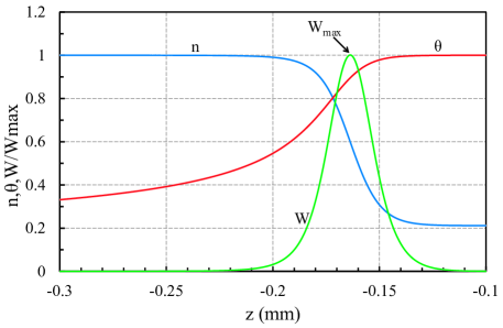
Figure 2: (Color online) Profile of the stationary deflagration front in a crystal of nanomagnets of Mn₁₂-acetate. The front moves from right to left. The external magnetic field is $B_{z}=$0.5\text{\,}\mathrm{T}$$ and the final temperature is $T_{f}=$9.9\text{\,}\mathrm{K}$$, with $\beta=-13/3$.

The final temperature $T_{f}$ behind the front is found from the energy conservation,

$$E_{0}+Qn_{0}=E_{f}+Qn_{f},$$ (8)

where index $0$ corresponds to initially “cold” matter (left side in Fig. 2) and index $f$ corresponds to the final “hot” (right side) of the front. In the case of incomplete burning (i.e., $n_{f}\neq 0$), this equation is a transcendental one and must be solved numerically. We assume that the temperature behind the front $T_{f}$ is constant because the heat escape to an external heat sink for this particular configuration can be neglected. The time for the spin reversal of the entire sample at the slowest deflagration rate approximately is $t_{d}\approx L/U_{f}=$0.016\text{\,}\mathrm{s}$$. The characteristic time of cooling is $t_{c}\approx S/\kappa=$0.19\text{\,}\mathrm{s}$$ (for this assumption we have used the thermal diffusion constant from Ref. Vélez et al. (2014), $\kappa=$0.19\text{\,}\mathrm{m}^{2}\mathrm{/}\mathrm{s}$$, and surface area $S=$2.88\text{\times}{10}^{-6}\text{\,}\mathrm{m}^{2}$$). Note also that in Ref. Vélez et al. (2014), the time for the sample the return to the temperature of the bath was measured as $\sim$1\text{\,}\mathrm{s}$$. Therefore, since $t_{d}\ll t_{c}$, we will neglect cooling effects in this study.

To simplify further derivations we introduce dimensionless variables for the coordinate and temperature together with scaled activation and Zeeman energies,

$$\xi\equiv zL_{f},\quad\theta\equiv T/T_{f},\quad\Theta\equiv E_{a}/T_{f},\quad\Delta\equiv Q/T_{f}$$ (9)

and define

$$J\equiv\frac{Q\Theta^{\alpha}_{D}}{AT^{\alpha+1}_{f}},\quad\kappa\equiv\kappa_{0}\theta^{-\beta},\quad L_{f}\equiv\frac{\kappa_{0}T_{f}^{-\beta}}{U_{f}}.$$ (10)

Here, $L_{f}$ is a characteristic length of the problem. Then in the reference frame of the moving front the equations (4)–(5) form the dimensionless system

$$\begin{split}\frac{d\psi}{d\xi}&=\theta^{\beta}\psi-J\Lambda b_{z}ne^{-\Theta/\theta}\left(n-n_{\mathrm{eq}}\right),\\ \frac{d\theta}{d\xi}&=\psi\theta^{\beta-\alpha},\\ \frac{dn}{d\xi}&=-\Lambda e^{-\Theta/\theta}\left(n-n_{\mathrm{eq}}\right),\end{split}$$ (11)

where $\psi$ stands for the heat flux and $\Lambda=L_{f}\Gamma_{R}/U_{f}$ is an eigenvalue of the stationary front. The new variable $\psi$ allows us to write down the governing system as a set of first-order differential equations, which is important for stability analysis described in Sec. IV. In order to calculate the stationary profiles depicted in Fig. 2, we integrate the system (11) from the left, “cold” side towards the right, “hot” side, and the eigenvalue $\Lambda$ is found by this shooting method Modestov et al. (2009), matching the results of numerical integration to the analytical solution given by Eq. (8) for the final temperature.

It should be noted that the assumption of a stationary front is valid when the front thickness is much smaller than the length of the sample. The characteristic front width can be determined as the half-width of the energy release peak; from Fig. 2 we find that $L_{f}\approx$0.025\text{\,}\mathrm{mm}$$. The typical crystal size used in experiments is 1–$2\text{\,}\mathrm{mm}$ Vélez et al. (2014), which is almost two orders of magnitude larger than the front width. Consequently, there is enough room to form a steady propagating front of magnetic deflagration.

Another issue to mention is the ambiguity in determining the front velocity $U_{f}$. Resolving the stationary profiles, we compute the front eigenvalue $\Lambda$, however in order to find $U_{f}$ we need to know the value of $\kappa_{0}\Gamma_{R}$ according to expressions (10), as

$$\Lambda=\frac{\kappa_{0}\Gamma_{R}T_{f}^{-\beta}}{U_{f}^{2}}.$$ (12)

So far, the actual parameters $\kappa_{0}$ and $\Gamma_{R}$ have not been measured, and we estimate the relation $\kappa_{0}\Gamma_{R}$ by fitting the velocity to experimental data Hernández-Mínguez et al. (2005). The dependence of $\Gamma_{R}$ on the magnetic field has been the subject of many studies, see, e.g., Refs. Leuenberger and Loss (2000); Garanin and Jaafar (2010). In this paper, we interpolate $\Gamma_{R}(B)$ by fitting experimental data Hernández-Mínguez et al. (2005) (see Fig. 3) using a Gaussian function to model tunneling resonances as Jukimenko et al. (2014)

$$\Gamma_{R}(B)=\Gamma_{0}\left\{1+\sum_{i}a_{i}\exp\left[-b_{i}\left(\frac{B}{B_{i}}-1\right)^{2}\right]\right\},$$ (13)

where $B_{i}$ is the resonance magnetic field, $\Gamma_{0}$ is a constant, and parameters $a_{i}$, $b_{i}$ are the amplitude and the width of the resonance, respectively. According to experimental data Hernández-Mínguez et al. (2005) shown in Fig. 3, these parameters are calculated as

$$B_{1} =$0.92\text{\,}\mathrm{T}$, a_{1} =1.89, b_{1} =840,$$ (14)

$$B_{2} =$1.32\text{\,}\mathrm{T}$, a_{2} =2.61, b_{2} =870,$$

with the estimate $\kappa_{0}\Gamma_{0}\approx$4\text{\times}{10}^{5}\text{\,}{\mathrm{m}}^{2}\text{/}{\mathrm{s}}^{2}$$.

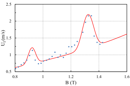
Figure 3: (Color online) Magnetic deflagration velocity $U_{f}$ for the planar front as a function of the longitudinal magnetic field $B_{z}$. The two peaks occur due to the tunneling resonance. The markers correspond to experimental data extracted from Ref. Hernández-Mínguez et al. (2005) and the line represents the fitted theoretical dependence.

III Analytical instability analysis within infinitely thin front

The propagation of the magnetic deflagration front is unstable Jukimenko et al. (2014) as any distortion of the front increases the magnetic field where the front bends, as shown in Fig. 4. This, in turn, leads to an increase of the front velocity, resulting in positive feedback. In this section, we will take a closer look at the front stability properties.

Figure 4: (Color online) Magnitude of the magnetic field in a 2D simulation for magnetic deflagration with a corrugated front. The external magnetic field is parallel to the $z$-axis, $B_{z}=$0.5\text{\,}\mathrm{T}$$. The front moves along the $z$-axis in the positive direction. The magnetization of the medium flips from $\mathbf{M}_{1}=(0;-M)$ in region 1 to $\mathbf{M}_{2}=(0;M)$ in region 2, with $\mu_{0}M=$0.05\text{\,}\mathrm{T}$$. The dipole field produced by the crystal results in an increase of the field at the tip of the humps.

In order to perform this analysis we need to make two assumptions. First, we assume that the magnetization of the particular nanomagnet is produced by the spins of the molecules, with the behavior of the spins described by Hamiltonian (1). The external magnetic field will significantly affect the eigenstates of Hamiltonian only when the second term in Eq. (1) becomes comparable to the first term, i.e., for an anisotropy field $B_{A}=2D/(g\mu_{B})$. For Mn₁₂-acetate, $B_{A}$ is of the order of $10\text{\,}\mathrm{T}$ Garanin and Chudnovsky (1997). In our study, we focus on fields strengths much lower than the anisotropy field, where the dependence of $\mathbf{M}$ on $\mathbf{B}$ is negligible, see Fig. 2 in Ref. Dion et al. (2013). Therefore, we suppose that the amplitude of the crystal magnetization $\mathbf{M}$ does not depend on the strength of the external field. Second, we assume that front width is infinitely thin, so that the profiles presented in Fig. 2 reduce to step functions, separating the cold and the hot regions of the crystal. We will remove these restrictions in the next section and consider the instability properties for a continuous front structure.

With respect to the front propagation and easy axis, multiple mutual orientations are possible. We consider the two principal cases: the front propagation is aligned with, Fig. 5(a), or perpendicular to, Fig. 5(b), the easy axis of the crystal.

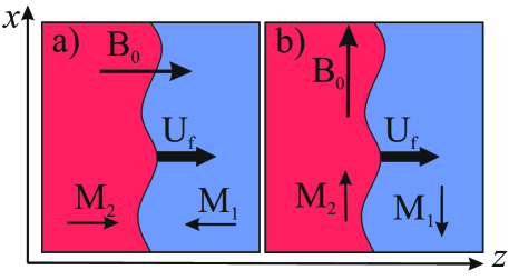
Figure 5: (Color online) Possible orientations of the front propagation vs. the crystal easy axis: (a) Most common geometry used in experiments, where the easy axis is parallel to the direction of the front propagation; (b) Hypothetical orientation of the crystal, where the easy axis is perpendicular to the direction of the front propagation. The external magnetic field $B_{0}$ is oriented along the easy axis of the crystal.

The position of a planar front, propagating with a constant velocity $U_{f}$, is given by $Z_{f}=U_{f}t$. The front is then perturbed with a superposition of Fourier modes written as

$$Z_{f}(x,t)=U_{f}t+\sum_{k}\widetilde{Z}_{k}\exp(ikx+\sigma t),$$ (15)

where $\sigma$ is the instability growth rate, $k=2\pi/\lambda$ is the wave number, and $\lambda$ is the wavelength of the perturbations. If $\mathrm{Re}(\sigma)>0$ the perturbations grow in time and the front becomes unstable; in the opposite case, $\mathrm{Re}(\sigma)<0$, the front is remains stable. The imaginary part of $\sigma$ leads to oscillations and pulsations of the front Modestov, Bychkov, and Marklund (2011a); in this paper we consider the case when $\mathrm{Im}(\sigma)=0$, such that $\sigma$ takes only purely real values.

We start with the case when the front propagates parallel to the easy axis and the magnetic field, Fig. 5(a). This is a common crystal orientation in experimental studies McHugh et al. (2007); Vélez et al. (2014); Decelle et al. (2009). Magnetization flips from $\mathbf{M}_{1}=(0;-M)$ in the cold region before the front to $\mathbf{M}_{2}=(0;M)$ in the hot region behind the front, see Fig. 5(a). The deformation of the front induces perturbations in the magnetic field,

$$\mathbf{B}_{z}=\mathbf{B}_{0}+\sum_{k}\widetilde{\mathbf{B}}_{k}(z)\exp(ikx+\sigma t).$$ (16)

The magnetic field inside the crystal is governed by the stationary Maxwell equations for nonconducting media,

$$\nabla\times\mathbf{H} =0, \nabla\cdot\mathbf{B} =0,$$ (17)

with the relation $\mathbf{B}/\mu_{0}=\mathbf{H}+\mathbf{M}$, where $\mu_{0}$ is the magnetic constant. Far from the front all the perturbations must vanish, such that the magnetic field perturbations along $z$ can be written as $\widetilde{\mathbf{B}}_{1,2}(z)\propto\exp(\mp kz)$. Boundary conditions for the magnetic field on the front interface are

$$\widehat{\mathbf{a}}_{n}\cdot\left[\mathbf{B}\right] =0, \widehat{\mathbf{a}}_{n}\times\left[\mathbf{H}\right] =0,$$ (18)

where $\left[F\right]\equiv F_{2}-F_{1}$ designates the difference of any value $F$ across the front and the normal vector to the perturbed front is $\widehat{\mathbf{a}}_{n}\equiv\widehat{\mathbf{a}}_{z}-\widehat{\mathbf{a}}_{x}\partial_{x}{Z}_{f}$.

Resolving Maxwell’s equations (17) together with the boundary conditions, we find the relation between the magnetic fields ahead and behind the front. Taking $z=0$ we find that

$$\widetilde{B}_{z1}=\widetilde{B}_{z2}=\mu_{0}Mk\widetilde{Z}_{f},$$ (19)

which leads to an increase of the magnetic field at the tip of the hump. Within the linear stability problem, the perturbation of the front velocity is given by $\partial_{t}\widetilde{Z}_{f}=U^{\prime}_{f}\widetilde{B}_{z}$, where $U^{\prime}_{f}\equiv dU_{f}/dB$ Jukimenko et al. (2014). It yields the dispersion relation in a very concise form as

$$\sigma=kU^{\prime}_{f}\mu_{0}M.$$ (20)

This result means that an infinitely thin magnetic deflagration front is unstable with respect to perturbations of all wavelength, since $\sigma>0$ for any $k$. Mathematically, this relation $\sigma\propto k$ is similar to the Darrieus-Landau instability Bychkov and Liberman (2000); Matalon (2007).

Next, we consider the crystal configuration where the front propagation is perpendicular to the easy axis of the crystal, Fig. 5(b). In this case, the magnetization varies as $\mathbf{M}_{1,2}=(\mp M;0)$ and the external magnetic field is given as $\mathbf{B}_{0}=\hat{\mathbf{a}}_{x}B_{0}$. Using the same approach as above, we obtain the dispersion relation

$$\sigma=-kU^{\prime}_{f}\mu_{0}M.$$ (21)

Hence such a configuration results in a stable propagation of the magnetic deflagration wave.

Characteristic values of the relative strength of the instability $\sigma/U_{f}k$ may vary significantly for different materials, depending on the magnetization $M$ and front velocity sensitivity $U^{\prime}_{f}$. We therefore expect noticeable magnetic instabilities in two cases, when either $M$ or $U^{\prime}_{f}$ are high. Strong magnetization can be found in ferromagnetic materials, so this instability might affect propagation of the domain walls. In magnetic nanomagnets, the magnetization is relatively weak, $\mu_{0}M\sim$0.05\text{\,}\mathrm{T}$$ Garanin and Shoyeb (2012), but the velocity slope $U^{\prime}_{f}$ theoretically can reach infinite values at the tunneling resonances Garanin (2013).

IV Stability analysis accounting for the internal front structure

In Sec. III, we found that the magnetic deflagration front is unstable in the infinitely thin front limit. However, such a method does not provide any characteristic length scale for the instability nor the strength of the instability or its dependence on the external magnetic field. Here, we investigate the instability properties taking into account a finite front width and the continuous structure of the deflagration front obtained in Sec. II.

For a finite front thickness, the magnetic field $\mathbf{B}$, together with the all other variables, changes continuously within the front. We introduce the magnetic vector potential $\mathbf{A}$ defined from $\mathbf{B}=\nabla\times\mathbf{A}$, such that the first Maxwell equation $\nabla\cdot\mathbf{B}=0$ is satisfied automatically. For a planar front, the vector potential has only one component $\mathbf{A}=(0,A(x,z),0)$ and for uniform field $B_{0}$ it reduces to $\mathbf{A}=(0,xB_{0},0)$. Consequently, the magnetic field components are

$$B_{x} =-\frac{dA}{dz}, B_{z} =\frac{dA}{dx}.$$ (22)

The second Maxwell equation $\nabla\times\mathbf{H}=0$ can be rewritten as

$$\nabla^{2}A-2\mu_{0}M_{0}\frac{dn}{dx}=0,$$ (23)

where we assume that the magnetization changes proportionally to the ratio of the metastable molecules $\mathbf{M}=(0,0,M_{0}(2n-1))$. We introduce the dimensionless magnetic potential defined as $a\equiv A/(L_{f}\mu_{0}M_{0})$ and a new variable $\chi\equiv i\,da/d\xi$ in order to have differential equations of the first order only.

Next, we apply a small perturbation so that every variable is written in as $f(z,x,t)=f(z)+\tilde{f}(z)\exp(ikx+\sigma t)$. After straightforward calculations, the linearized equations (11) and (23) can be written in matrix form as

$$\frac{d}{d\xi}\mathbf{v}=\mathbf{D}\mathbf{v},$$ (24)

where $\mathbf{v}=\left(\tilde{\theta},\tilde{n},\tilde{\psi},\tilde{a},\tilde{\chi}\right)^{T}$ is the vector of perturbations. $\mathbf{D}=\mathbf{D}\left(\xi,S,K\right)$ is a $5\times 5$ matrix of the coefficients of the system of differential equations,

$$\mathbf{D}=\begin{pmatrix}(\beta-\alpha)\psi\theta^{\beta-\alpha-1}&0&\theta^{\beta-\alpha}&0&0\\ -\Phi&-S-W&0&D_{24}&0\\ D_{31}&-WJ&\theta^{\beta}&D_{34}&0\\ 0&0&0&0&1\\ 0&-2K&0&K^{2}&0\\ \end{pmatrix},$$ (25)

where the matrix components are

$$D_{24} \equiv K\left[W\frac{C_{1}}{\theta}(n-n_{\mathrm{eq}})-\frac{C_{2}}{b_{0z}}\right],$$ (26)

$$D_{31} \equiv\beta\psi\theta^{\beta-1}-JW\frac{\Theta}{\theta^{2}}\left(n-n_{\mathrm{eq}}-n^{2}_{\mathrm{eq}}\frac{\Delta}{\Theta}e^{\Delta/\theta}\right)$$

$$\quad+S\theta^{\alpha}+K^{2}\theta^{\alpha-\beta},$$

$$D_{34} \equiv\frac{K}{b_{z}}\left[W(n-n_{\mathrm{eq}})\left(1+b_{0z}\frac{C_{1}}{\theta}\right)-C_{2}\right],$$

with

$$W \equiv\Lambda e^{-\Theta/\theta}, C_{1} \equiv\frac{g\mu_{B}S_{z}}{T_{f}\mu_{0}M_{0}}, C_{2} \equiv Wn^{2}_{\mathrm{eq}}$$

introduced for brevity. In the equations above, $b_{0z}\equiv\mu_{0}M_{0}B_{0z}$ is a dimensionless external magnetic field, and $S\equiv\sigma\Gamma_{0}$ and $K\equiv kL_{f}$ are the scaled instability growth rate and perturbation wave number, respectively. Some of the matrix coefficients in (25) are known from the stationary profile, while the others depend on $S$ and $K$ as parameters.

In order to find the instability dispersion relation $S(K)$, we apply the same method as in similar studies of instabilities Modestov et al. (2009); Modestov, Bychkov, and Marklund (2011a). First, we search for solutions to the system (24) in the uniform regions, where all the coefficients in matrix $\mathbf{D}$ are constant. In this case the perturbations decay exponentially as

$$\lim_{\xi\rightarrow\pm\infty}\mathbf{v}=\mathbf{v}_{i}\exp{\left(\mu_{i}\xi\right)},$$ (27)

where the $\mu_{i}$ are the so-called system modes and $\mathbf{v}_{i}$ are constant perturbation amplitudes. Substituting Eq. (27) into Eqs. (24), we obtain

$$\mathbf{D}\mathbf{v}=\mu\mathbf{v}.$$ (28)

We compute the eigenvalues $\mu_{i}$ and the corresponding eigenvectors $\mathbf{v}_{i}$. We consequently obtain five modes for the cold and the hot sides of the front, although not all of them are physical. In order to pick out the physical eigenvectors, we use the condition that perturbations must vanish far from the front as $\lim_{\xi\rightarrow\pm\infty}\mathbf{v}\rightarrow 0$. In other words, we consider eigenvectors $\mathbf{v}_{i}$ for which $\mu_{i}>0$ at $\xi\rightarrow-\infty$ or $\mu_{i}<0$ at $\xi\rightarrow+\infty$. If the problem is self-consistent, there will be exactly five modes $\mu_{i}$ satisfying these conditions, usually three modes on one side and two on the other.

After that we integrate Eqs. (24) from the front boundaries using $\mathbf{v}_{i}$ as boundary conditions. We match the results of the integration at the point of maximal energy release $W_{\mathrm{max}}$ (shown in Fig. 2). Generally speaking this matching point can be chosen in a different way without affecting the final results, however the current choice minimizes the numerical integration errors Modestov et al. (2009). At this point the integrated amplitudes constitute a matrix and the dispersion relation $S=S(K)$ is obtained when the matrix determinant becomes equal to zero.

V Results and discussion

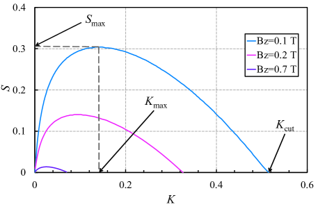
Figure 6: (Color online) Dimensionless instability growth rate versus the dimensionless wave number for different magnetic fields. Values $K_{\mathrm{cut}}$, $K_{\mathrm{max}}$, and $S_{\mathrm{max}}$ are shown only for the dispersion relation for $B_{z}=$0.1\text{\,}\mathrm{T}$$.

The dispersion relation $S=S(K)$ is shown in Fig. 6, for several magnitudes of external magnetic field. It has a parabola-like shape similar to the one obtained for the Darrieus-Landau instability in combustion and laser ablation Landau and Lifshitz (1989); Bychkov and Liberman (2000); Modestov et al. (2009). In the region of small wave numbers the instability displays a strong increase of the growth rate against the variation of the wave number. Then, at a certain wave number $K_{\mathrm{max}}$, the instability growth rate reaches its maximum $S_{\mathrm{max}}$. After that, the instability becomes weaker until it vanishes at $K_{\mathrm{cut}}$. As in the case of the Darrieus-Landau instability, the stabilization is attributed to the final front width due to thermal conduction.

Another important outcome from Fig. 6 is that the instability is stronger for relatively weak fields. This can be qualitatively explained in the following way. The instability is caused by the dipole field created by the crystal magnetization. In our model this magnetization does not depend on the external magnetic field. Hence for weak fields ($B_{0}<$0.1\text{\,}\mathrm{T}$$) the magnetization at the curved front creates a relatively strong dipole field as compared to the external field. This, in turn, increases the front velocity driving the instability to grow further. On the other hand, for high external fields, the increase due to crystal magnetization is relatively weak, leading to a much smaller increase of the front velocity.

The influence of the magnetic field is better shown in Figs. 7 and 8, where we present the maximum instability growth rate as well as the cutoff wavelength and wavelength at the maximum as a function of the external magnetic field. In both these figures we use dimensional quantities, allowing a simpler comparison to experiments. As discussed above, we observe strong decrease of the instability growth rate with respect to the magnetic field, Fig. 7. The two peaks correspond to quantum tunneling at resonant magnetic fields. As follows from Fig. 7, the instability is the strongest and can be observed in the region of very small fields. On the other hand, in Fig. 8 we see that the wavelength $\lambda_{\mathrm{max}}$ corresponding to the maximal growth rate can be rather high in that range of magnetic field.

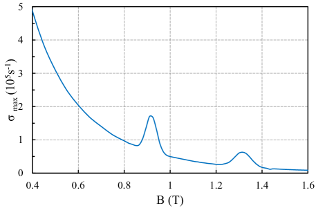
Figure 7: (Color online) Maximum of the instability growth rate versus magnetic field for Mn₁₂-acetate.

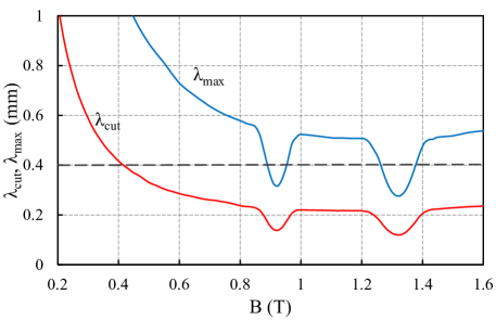
Figure 8: (Color online) Cutoff wavelength and wavelength at the maximum, for Mn₁₂-acetate. The horizontal dashed gray line shows the typical sample width $0.4\text{\,}\mathrm{mm}$ in experiments Vélez et al. (2014).

It is important to emphasize that the scaling parameters $\kappa_{0}$ and $\Gamma_{0}$ are difficult to measure directly. It is also difficult to estimate these quantities using theoretical models. For instance, values of $\kappa_{0}=$3\text{\times}{10}^{-2}$T^{-13/3}$, $1.5\text{\times}{10}^{-5}$, and $$3\text{\times}{10}^{-9}$T^{13/3}$, in units of ${\mathrm{m}}^{2}\text{/}\mathrm{s}$, were found using different heat transfer models Vélez et al. (2014). Here, we used $\Gamma_{0}=$1\text{\times}{10}^{7}\text{\,}{\mathrm{s}}^{-1}$$ and $\kappa_{0}=$0.04\text{\,}{\mathrm{m}}^{2}\text{/}\mathrm{s}$$ in Figs. 7 and 8. Our analysis could be used to measure the product $\kappa_{0}\Gamma_{0}$, as the instability of the magnetic deflagration can be detected in two ways: (i) direct observation, using magneto-optical imagining Villuendas et al. (2008), where the planar front becomes corrugated with a parabola-like shape as predicted by numerical simulations Jukimenko et al. (2014); Garanin (2013); (ii) the instability can be detected by measuring deflagration speed, as a curved front propagates faster then a planar one Jukimenko et al. (2014).

A stationary propagation of the curved front was predicted and explained within non-linear theory in Ref. Jukimenko et al. (2014). Similar results were obtained using direct numerical simulation in Ref. Jukimenko et al. (2014) and Ref. Garanin (2013). Importantly, such an instability occurs regardless of the presence of resonances. Meanwhile, turbulent propagation of the front observed in Ref. Garanin (2013) occurs when the field is resonant (where the theoretical model predicts nearly infinitely fast relaxation). Propagation of the front at resonant field strengths (when the relaxation rate is extremely high) must be taken as a separate problem and is not considered here. Perturbations with different $k$ have different growth rates, see Eq. (20). Therefore, the perturbation with highest growth rate $\sigma$ develops faster and leads to a stationary, curved front (see the numerical simulations in Ref. Jukimenko et al. (2014)).

The growth rate stands for the characteristic time needed for the instability to develop from a planar front to a stationary, curved front. For a possible observation of the instability, this time should be much smaller than the time of propagation of the magnetic deflagration front within the crystal. In particular, recent experiments Vélez et al. (2014) were performed with a sample size of $1.6\times$0.4\text{\,}\mathrm{mm}$$ with $B_{z}=$0.4\text{\,}\mathrm{T}$$, corresponding to a typical time of about $6.4\text{\times}{10}^{-3}\text{\,}\mathrm{s}$. Fig. 7 predicts $1/\sigma=$2\text{\times}{10}^{-4}\text{\,}\mathrm{s}$$ for such a field magnitude, hence the instability might have enough time to develop. However, the wavelength where the growth rate is maximal is larger than the sample width, depicted as a dashed line in Fig. 8, which leads to a decrease of the instability growth rate, since the wavelength of the perturbation cannot exceed the width of the sample. In addition, this means that the front may be only slightly curved.

Under restrictions of the size of the sample, the resonant magnetic field makes the observation of the magnetic instability more plausible. We see that the resonance enhances the instability growth rate in two ways. First it increases the growth rate $\sigma_{\mathrm{max}}$, as demonstrated by the peaks in Fig. 7. Second, it decreases the cutoff wavelength and the wavelength at the maximum (Fig. 8), such that the estimated values are within the range of the dimensions of the crystal. In addition to that, the amplitude of the resonance can be increased significantly by applying a transverse magnetic field, effectively increasing $\Gamma_{0}$. If the instability becomes strong enough, acceleration of the deflagration front can create a weak shock wave ahead of the front, which might lead to the deflagration-to-detonation transition Modestov, Bychkov, and Marklund (2011b). In the weak detonation regime, the front propagates at the speed of sound, and such a spin reversal phenomena has already been observed experimentally near a resonance Decelle et al. (2009).

VI Conclusion

We have studied the front instability in magnetic deflagration and found that it behaves in a similar fashion to the Darrieus-Landau instability in combustion. That is, in the limit of an infinitely thin front, the instability has a positive growth rate at all wavelengths. The dispersion relation of the growth rate as a function of the instability wave number is also similar to that of the Darrieus-Landau instability. The case of a finite-width front was explored numerically, and we found that the instability should be observable in current experimental setup, in particular close to a tunneling resonance, the latter resulting in a smaller value of the wavelength at which the instability will have the highest growth rate.

Analysing the effect of the direction of propagation of the front with respect to the easy axis, we showed that the instability would not grow for a perpendicular front. We suggest two different experimental setups (a) and (b), see Fig. 5. Theory predicts an unstable front in case (a), resulting in a faster propagation of the front as result, and a stable front in case (b). By comparing velocities of the magnetic deflagration of these two different geometries one can verify the presence of the instability.

Signatures of the presence of the instability might also explain some previous experimental results. For instance, for strong longitudinal fields, the velocities recorded in the experiments are higher than the theoretical predictions Vélez et al. (2014), which could be explained by the effect of the instability on front speed. (Note that while the front would be curved due to the instability, the propagation speed of the curved front will also be steady. Jukimenko et al. (2014)) Likewise, the front broadening also observed in Ref. Vélez et al. (2014) could be explained by the front instability.

Finally, we showed that there is a relation between the instability and the front velocity $U_{f}$, diffusion constant $\kappa_{0}$, and the thermal relaxation rate $\Gamma_{R}$. Experimental studies of the instability could help measure the values of the latter two parameters.