Phosphorene confined systems in magnetic field, quantum transport, and superradiance in the quasi-flat band

Abstract

Spectral and transport properties of electrons in confined phosphorene systems are investigated in a five hopping parameter tight-binding model, using analytical and numerical techniques. The main emphasis is on the properties of the topological edge states accommodated by the quasi-flat band that characterizes the phosphorene energy spectrum.

We show, in the particular case of phosphorene, how the breaking of the bipartite lattice structure gives rise to the electron-hole asymmetry of the energy spectrum. The properties of the topological edge states in the zig-zag nanoribbons are analyzed under different aspects: degeneracy, localization, extension in the Brillouin zone, dispersion of the quasi-flat band in magnetic field. The finite-size phosphorene plaquette exhibits a Hofstadter-type spectrum made up of two unequal butterflies separated by a gap, where a quasi-flat band composed of zig-zag edge states is located. The transport properties are investigated by simulating a four-lead Hall device (importantly, all leads are attached on the same zig-zag side), and using the Landauer-Büttiker formalism. We find out that the chiral edge states due to the magnetic field yield quantum Hall plateaus, but the topological edge states in the gap do not support the quantum Hall effect and prove a dissipative behavior. By calculating the complex eigenenergies of the non-Hermitian effective Hamiltonian that describes the open system (plaquette+leads), we prove the superradiance effect in the energy range of the quasi-flat band, with consequences for the density of states and electron transmission properties.

I Introduction

The very recent revival of the black phosporene physics comes from the technical possibility to obtain monolayers, known as phosphorene, with specific topological properties. Phosphorene is a quasi-2D structure organized as a puckered hexagonal lattice, the top and side views being shown in Fig.1a and Fig.1b, respectively. One may think that, due to the structural similarity, the electron properties of phosphorene are resembling those of graphene. However, in contradistinction to graphene, the phosphorene is an anisotropic direct gap semiconductor, much more attractive for electronic devices. Beside the monolayered structure, multilayers of black phosporous are also studied, mainly in order to control the band gap, in the perspective of a potential application for field-effect transistors.

The phosphorene ribbon geometry (especially, with zig-zag edges) is also conceptually interesting since, instead of the semi-metallic spectrum of graphene, distinguished by a flat band at $E=0$, and extending between the points K and K’ in the Brillouin zone (BZ), the phosphorene shows well-separated valence and conduction bands and a quasi-flat band in the middle of the gap, composed of edge states that exists at any momentum $k\in BZ$.

In the tight-binding model, the phosphorene lattice is described by five hopping integrals $t_{1},t_{2},..,t_{5}$ Katsnelson , which induce the significant differences in the electron spectrum that are noticed when compared to graphene. The model points out also the anisotropy of the energy spectrum: both the top of the valence band and the bottom of the conduction band look quadratically as function of $k_{y}$ , but nearly linear as function of $k_{x}$ (Dirac-like) (see Fig.2), situation which is described in terms of hybrid Dirac spectrum Montambaux ; Goerbig . The hopping integral $t_{4}$ plays a distinctive role as it connects sites of the same kind on the hexagonal lattice, breaking the bipartitism of the lattice, and, as a consequence, the electron-hole symmetry of the energy spectrum is also broken Mielke . As an additional effect due to $t_{4}$, we shall see in Sec.II that the edge states, organized in a perfect flat band at $t_{4}=0$, undergoes dispersion in the case of nonvanishing $t_{4}$.

The properties of the macroscopically degenerate flat (quasi-flat) bands composed of edge states in confined systems (ribbon or finite-size plaquette) attract much attention nowadays, and phosphorene presents a serious advantage coming from the existence of a gap that protects the quasi-flat band, such that its properties can be evidenced in a cleaner way. The study of the spectral and transport properties in the magnetic field, and the response of the quasi-flat band to the invasive contacts of a Hall device, identified as a superradiant phenomenon, are a topic of our paper.

Similar to graphene, the confined phosphorene exhibits two types of edge states: i) the chiral edge states generated by a strong perpendicular magnetic field $\mathcal{B}$, and supporting the quantum Hall effect (QHE), and ii) the edge states typical to the zig-zag boundaries in the hexagonal lattice, which exists even in the absence of the magnetic field. The last ones, which will be called topological edge states Ezawa , are non-chiral and remain like that even at $\mathcal{B}\neq 0$. Obviously, they do not show QHE, but show longitudinal conductance, i.e., they have a dissipative character.

The transport calculations assume the knowledge of the full Hamiltonian of the open system consisting of the finite-size system of interest (namely, the phosphorene plaquette) and the semi-infinite leads. Technically speaking, one uses actually an effective Hamiltonian obtained by formal elimination of the degree of freedom of the leads, however, as the price to be paid, the result is a non-Hermitian Hamiltonian with complex eigenvalues. The method of non-Hermitian Hamiltonian has been used for the calculation of transport properties of the quantum dots in the Landauer-Büttiker formalism (see for instance Moldoveanu ), but also in the localization-delocalization problem in the 1D non-Hermitian Anderson model Nelson ; Khoruz ; Celardo . In these two different problems, the non-hermicity arises from different sources, however we do not enter here such peculiar aspects.

In the phosphorene confined system, the complex eigenvalues of the effective Hamiltonian in the energy range of the quasi-flat band, corroborated by the calculation of the electron transmission, density of states and local density of states make evident a specific superradiant behavior of the topological edge states. (We remind that the superradiance consists in the segregation of eigenenergies and overlapping of some resonances, the process being controlled by the lead-system coupling Nesterov .) For instance, the density of states of the quasi-flat band exhibits a miniband structure, each miniband behaving as a 1D-conducting channel with the conductance $G=e^{2}/h$. These aspects are discussed in Sec.IV.

Some quantum transport aspects in phosphorene were very recently revealed. The quantum Hall effect and spin splitting of the Landau levels (LL) were observed in KaiChang ; Likai , and also Shubnikov-deHaas oscillations of the longitudinal resistance were found in Likai1 . The transport anisotropy, reflecting the structural one, was shown experimentally by measuring the angle dependence of the drain current HanLiu or by the non-local response Levitov . The strain-induced modifications of the phosphorene band structure were studied in Neto ; Fey . The field effect transistor is also the topic of Wu ; Likai2 .

The paper is organized as follows. Sec.II presents the tight-binding Hamiltonian, Peierls phases in magnetic field and discusses the question of electron-hole symmetry breaking. Sec.III is devoted to the study of the phosphorene ribbon in the magnetic field, as an extension of Ezawa analysis at $\mathcal{B}=0$. Sec.IV deals with the spectral and transport properties of the phosphorene mesoscopic plaquette, showing the specific features of the quantum Hall effect in the bands, and the properties resulting from the superradiance effect in the quasi-flat band. The summary and conclusions can be found in the last section.

II The tight-binding model and electron-hole symmetry breaking in phosphorene

Similar to graphene, the unit cell contains two atoms called $A$ and $B$, however the phosphorene tight-binding Hamiltonian is more complicated as it contains five hopping integrals to nearest and next-nearest neighbors. In order to write down the Hamiltonian we define the creation and annihilation operators $a^{\dagger}_{nm},a_{nm},b^{\dagger}_{nm},a_{nm}$, where $n$ and $m$ are cell indexes along the Ox- and Oy-axis, respectively. In the presence of a perpendicular magnetic field, which will be described by the vector potential $\vec{\mathcal{A}}=(-\mathcal{B}y,0,0)$, some of the hopping integrals acquire the Peierls phase expressed by the circulation of the vector potential along the trajectory connecting the two end points :

$$\phi_{AB}=\frac{2\pi}{\Phi_{0}}\int_{A}^{B}\vec{\mathcal{A}}d\vec{l}=-\frac{2\pi B}{\Phi_{0}}\int_{x_{A}}^{x_{B}}y(x)dx.$$ (1)

Much attention should be paid to the calculation of the phases since the angle $\beta$ describing the deviation from the perfect flat 2D lattice (see Fig.1b) enter also the calculation. Since the hopping integral $t_{4}$ plays the special role mentioned in the introduction, we separate the terms proportional to this parameter, and the spinless tight-binding Hamiltonian of the phosphorene lattice under perpendicular magnetic field will be written as follows:

$$H = H^{0}+H^{4},$$

$$H^{0} = \sum_{nm}E_{a}a^{\dagger}_{nm}a_{nm}+E_{b}b^{\dagger}_{nm}b_{nm}+t_{1}\big{(}e^{i\phi_{1}}a^{\dagger}_{n+1m}+e^{-i\phi_{1}}a^{\dagger}_{nm}\big{)}b_{nm}+t_{2}a^{\dagger}_{nm+1}b_{nm}$$

$$+ t_{3}\big{(}e^{i\phi_{3}}a^{\dagger}_{nm+2}+e^{-i\phi_{3}}a^{\dagger}_{n-1m+2})b_{nm}+t_{5}a^{\dagger}_{n+1m-1}b_{nm}+H.c.~{},$$

$$H^{4} = \sum_{nm}t_{4}\big{(}e^{i\phi_{4B}}b^{\dagger}_{nm+1}+e^{-i\phi_{4B}}b^{\dagger}_{n-1m+1}\big{)}b_{nm}$$ (2)

$$+ t_{4}\big{(}e^{i\phi_{4A}}a^{\dagger}_{nm+1}+e^{-i\phi_{4A}}a^{\dagger}_{n-1m+1}\big{)}a_{nm}+H.c.,$$

where $E_{a}$ and $E_{b}$ are the atomic energies at the sites $A$ and $B$, respectively, and , according to Katsnelson , $t_{1}=-1.220eV,t_{2}=3,665eV,t_{3}=-0.205eV,t_{4}=-0.105eV,t_{5}=-0.055eV$. Since the hopping parameters are given in electron-volts, all the quantities in the paper having the dimension of energy will be measured in the same units.

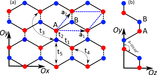
Figure 1: (Color online) (a) Schematic representation of phosphorene lattice with two types of edges, zig-zag (along the $\textbf{O}_{x}$ direction) and armchair (along the $\textbf{O}_{y}$ direction); $t_{1},t_{2},t_{3},t_{4},t_{5}$ are the hopping amplitudes that connect the lattice sites; A (red) and B (blue) index the two types of atoms, and the dashed blue lines represent the unit cell with $\textbf{a}_{1}$ and $\textbf{a}_{2}$ as unit vectors. (b) The projection of the lattice on the yz-plane. The number of lattice sites is $7\times 4$.

In the chosen gauge of the vector potential, only three hopping integrals acquire a Peierls phase in magnetic field, namely $t_{1},t_{3}$ and $t_{4}$. For instance, $\phi_{1}(m)$ in Eq.(1) is the Peierls phase corresponding to the hopping from the site B in the cell (n,m) to the site A in the next cell (n+1,m), and equals:

$$\phi_{1}(m)=2\pi\frac{\mathcal{B}}{\Phi_{0}}\int_{B_{nm}}^{A_{n+1,m}}y(x)dx=-2\pi\frac{\Phi}{\Phi_{0}}\frac{1}{6}\big{(}(m-1)(1+2sin\beta)-\frac{1}{2}\big{)}.$$

Similarly, the other phases in Eq.(2) are Note-phase ,

$$\phi_{3}(m) = -2\pi\frac{\Phi}{\Phi_{0}}\frac{1}{6}\big{(}m(1+2sin\beta)-\frac{1}{2}\big{)}$$

$$\phi_{4A}(m) = -2\pi\frac{\Phi}{\Phi_{0}}\frac{1}{6}(m-\frac{1}{2})(1+2sin\beta)$$

$$\phi_{4B}(m) = -2\pi\frac{\Phi}{\Phi_{0}}\frac{1}{6}\big{(}(m-\frac{1}{2})(1+2sin\beta)+1\big{)},$$

where $\Phi/\Phi_{0}$ is the magnetic flux through the hexagonal cell measured in quantum flux units, and $\beta$ is the angle shown in Fig.1b. One notices that the phases $\phi_{4A}$ and $\phi_{4B}$ acquired by $t_{4}$ along the A-A and B-B link, respectively, are different.

The spectral properties of the Hamiltonian (2) can be studied under different boundary conditions describing different geometries as the infinite sheet, the ribbon or the finite plaquette. The phoshorene infinite sheet can be simulated assuming periodic boundary conditions along the both directions $Ox$ and $Oy$. Let us consider first the case $\mathcal{B}=0$, and use the Fourier transform of the creation and annihilation operators:

$$a_{nm}=\sum_{\vec{k}}a_{\vec{k}}e^{i\vec{k}\vec{R}_{nm}},~{}~{}b_{nm}=\sum_{\vec{k}}b_{\vec{k}}e^{i\vec{k}\vec{R}_{nm}},~{}~{}\vec{R}_{nm}=n\vec{a}_{1}+m\vec{a}_{2},$$ (3)

which helps in writing the Hamiltonian as a $2\times 2$ matrix in the momentum space $\vec{k}=(k_{x},k_{y})$:

$$H=\sum_{\vec{k}}H^{0}_{\vec{k}}+H^{4}_{\vec{k}}=\sum_{\vec{k}}\left(\begin{array}[]{cc}a^{\dagger}_{\vec{k}}{}&b^{\dagger}_{\vec{k}}\end{array}\right)\left(\begin{array}[]{ccc}T^{4}(\vec{k})&T^{0}(\vec{k})\\ T^{0*}(\vec{k})&T^{4}(\vec{k})\end{array}\right)\left(\begin{array}[]{c}a_{\vec{k}}\\ b_{\vec{k}}\\ \end{array}\right),$$ (4)

with

$$T^{0}(\vec{k}) = t_{1}(1+e^{-i\vec{k}\vec{a}_{1}})+t_{2}e^{-i\vec{k}\vec{a}_{2}}+t_{3}(e^{-i2\vec{k}\vec{a_{2}}}+e^{i\vec{k}\vec{a_{1}}-i2\vec{k}\vec{a_{2}}})+t_{5}e^{-i\vec{k}\vec{a_{1}}+i\vec{k}\vec{a_{2}}}$$

$$T^{4}(\vec{k}) = 2t_{4}(cos\vec{k}\vec{a_{2}}+cos\vec{k}(\vec{a_{1}}-\vec{a_{2}})).$$ (5)

In approaching the question of spectrum symmetries, we remind that the electron-hole symmetry of an energy spectrum holds if there exists an operator $\mathcal{P}$ that anticommutes with the Hamiltonian, $\{H,\mathcal{P}\}_{+}=0$. Indeed, it is quite straightforward to see that, if $E$ is an eigenvalue, $H\Psi_{E}=E\Psi_{E}$, then the energy $-E$ belongs also to the spectrum, the corresponding eigenfunction being $\tilde{\Psi}_{-E}=\mathcal{P}\Psi_{E}$. For our specific problem of phosphorene, let us consider the operator

$$\mathcal{P}=\sum_{\vec{k}}a^{\dagger}_{\vec{k}}a_{\vec{k}}-b^{\dagger}_{\vec{k}}b_{\vec{k}}~{}.$$ (6)

Obviously, this operator anticommutes with $H^{0}$, attesting that the energy spectrum of $H^{0}$ is electron-hole symmetric, $\{E_{k}^{0},-E_{k}^{0}\}\in Sp$. However, $\mathcal{P}$ does not anticommute with the total Hamiltonian $H^{0}+H^{4}$, the result being proportional to $t_{4}$. One concludes that the phosphorene spectrum is electron-hole symmetric if $t_{4}=0$, i.e, when one forgets about the hopping to the next-nearest neighbors, but it is not necessarily symmetric otherwise.

The energy spectrum of the Hamiltonian (4) can be obtained analytically from the characteristic equation

$$\begin{vmatrix}E-T^{4}(\vec{k})&T^{0}(\vec{k})\\ T^{0*}(\vec{k})&E-T^{4}(\vec{k})\\ \end{vmatrix}=0,$$ (7)

resulting a two-band spectrum of semiconducting type, with the eigenvalues

$$E_{\pm}(\vec{k})=T^{4}(\vec{k})\pm|T^{0}(\vec{k})|.$$ (8)

The above equation confirms that for $t_{4}=0$ the spectrum becomes symmetric $E=\pm|T^{0}(\vec{k})|$, with a direct gap at the $\Gamma$ point equal to $\Delta=2|T^{0}(0)|=2(2t_{1}+t_{2}+2t_{3}+t_{5})$, which is Ezawa’s result Ezawa . On the other hand, Eq.(8) proves that a nonvanishing $t_{4}$ shifts the whole spectrum with $4t_{4}$, such that the electron-hole symmetry around $E=0$ is lost. One concludes that the spectral asymmetry in phosphorene is the consequence of the hopping parameter $t_{4}$, which connects sites of the same type and violates in this way the bipartitism of the lattice.

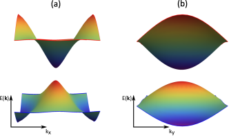
Figure 2: (Color online) The energy spectrum of the phosphorene lattice with periodic boundary conditions. The anisotropy of the spectrum around the $\Gamma$ point can be observed: (a) the energy dispersion along the $k_{x}$-axis shows the Dirac-like behavior, and (b) energy dispersion along the $k_{y}$-axis shows the Schrödinger-like behavior.

The eigenvalues Eq.(8) are displayed in Fig.2, where three aspects have to be noticed: the presence of the gap, the strong anisotropy, and the electron-hole asymmetry of the bands. As explained in Montambaux , the first two properties occur in the hexagonal-type lattice as soon as $t_{1}\neq t_{2}$, even neglecting the other hopping parameters in the Hamiltonian.

The Hofstadter spectrum generated by a perpendicular magnetic field is also very specific, consisting of two unequal butterflies separated by a gap. There is no agreement yet on the field dependence of the Landau levels, as in KaiChang ; Pereira the dependence is linear, while in Ezawa1 the dependence is $\sim~{}\mathcal{B}^{2/3}$. In Fig.3 we show the numerically calculated Hofstadter spectrum of a finite (mesoscopic) plaquette, which exhibits a supplementary band in the middle accommodating the edge states KaiChang1 . The narrow width of the band, and the weak dependence on the magnetic field should be noticed. One has to observe that the spectrum misses the known periodicity with the magnetic flux $E(\Phi+\Phi_{0})=E(\Phi)$, which is met in the case of the 2DEG in perpendicular magnetic field. This comes from the presence of three different Peierls phases in the Hamiltonian (2). The case of the phosphorene finite plaquette will be discussed in Sec.III.

The Hofstadter-type spectrum in Fig.3 suggests new physical properties of the edge states, and stimulates a more extensive study of the phosphorene mesoscopic systems. They are simulated in the tight-binding model by imposing vanishing boundary conditions for the wave function all along the perimeter (the case of the finite-size plaquette) or only along two parallel zig-zag edges (the ribbon case).

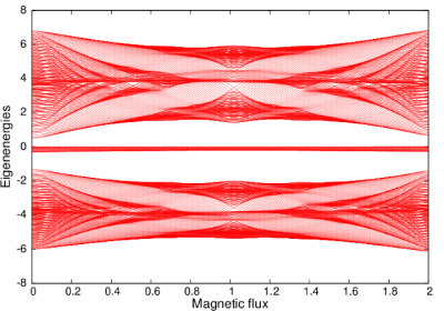
Figure 3: (Color online) The Hofstadter spectrum of the finite phosphorene lattice. The quasi-flat band which accommodates topological edge states can be noticed in the gap. The number of lattice sites is $21\times 20$, and the magnetic flux is measured in flux quanta $h/e$.

The phosphorene ribbon in the absence of the magnetic field is discussed in Ezawa ; Fazileh ; Carvalho , where it is shown that the zig-zag edges induce eigenvalues in the middle of the gap. The band is perfectly flat (i.e., independent of the momentum $k$) if $t_{4}=0$, and get a slight dispersion otherwise. At a given $k$, there are two quasi-degenerate states which become perfectly degenerate in the limit of wide ribbons (similar to the case of graphene).

The next section is devoted to the spectral properties of phosphorene ribbon in the presence of the magnetic field, in which case some new aspects of interest can be proved even analytically.

III Spectral properties of the phosphorene ribbon in magnetic field

Let us consider the Hamiltonian (2) and impose two edges parallel to the zig-zag chains at m=1 and m=M, but keeping periodic boundary conditions along the x-direction. The Fourier transform along the x-direction gives rise to the following Hamiltonian for the ribbon geometry (where $k$ stands for $k_{x}$):

$$\hskip-28.45274ptH = \sum_{k}H^{0}(k)+H^{4}(k),$$

$$H^{0}(k) = \sum_{m=1}^{M}E_{a}a^{\dagger}_{km}a_{km}+E_{b}b^{\dagger}_{km}b_{km}+t_{1}\big{(}e^{i(\phi_{1}-k)}+e^{-i\phi_{1}}\big{)}a^{\dagger}_{km}b_{km}$$

$$+ t_{2}\sum_{m=1}^{M-1}a^{\dagger}_{km+1}b_{km}+t_{3}\sum_{m=1}^{M-2}\big{(}e^{i\phi_{3}}+e^{-i(\phi_{3}-k)}\big{)}a^{\dagger}_{km+2}b_{km}+t_{5}\sum_{m=1}^{M}e^{-ik}a^{\dagger}_{km-1}b_{km}+H.c.~{}~{}$$

$$H^{4}(k) = t_{4}\sum_{m=1}^{M-1}\big{(}e^{i\phi_{4B}}+e^{-i(\phi_{4B}-k)}\big{)}b^{\dagger}_{km+1}b_{km}+\big{(}e^{i\phi_{4A}}+e^{-i(\phi_{4A}-k)}\big{)}a^{\dagger}_{km+1}a_{km}+H.c.~{}.$$ (9)

In the case of vanishing magnetic field $\mathcal{B}=0$, the energy spectrum of the above Hamiltonian is described by Ezawa Ezawa . The numerical calculation takes into account all the five hopping integrals, but the analytical one considers $t_{3}=t_{5}=0$, while the parameter $t_{4}$ is considered perturbatively. The existence of a quasi-flat band in the gap, whose dispersion comes from $t_{4}$, is proved (see Eq.(22)in Ezawa ). We reobtain this result, which is shown in Fig.5(left), in order to be compared with the case of nonvanishing magnetic field in Fig.5.(right)

III.1 The quasi-flat band in magnetic field

The aim of this subsection is to elucidate the effect of the perpendicular magnetic field on the spectral properties of the edge states in the ribbon geometry. The formation of the quasi-flat band in the middle of the gap and the interesting degeneracy lifting due to the magnetic field are put forward both numerically and analytically.

Let us consider the atomic energies $E_{a}=E_{b}=0$, and the hopping integrals $t_{3}=t_{5}=0$ (as in Ref.5), but keep $\mathcal{B}\neq 0$. Then, $H^{0}(k)$ becomes:

$$H^{0}(k)=\sum_{m=1}^{M}t_{1}\big{(}e^{i(\phi_{1}-k)}+e^{-i\phi_{1}}\big{)}a^{\dagger}_{km}b_{km}+\sum_{m=1}^{M-1}t_{2}a^{\dagger}_{km+1}b_{km}+H.c.~{}.$$ (10)

For any momentum $k$, we look for the eigenfunctions of $H^{0}(k)$ as

$$|\Psi^{0}(k)\rangle=\sum_{m=1}^{M}(\xi^{A}_{km}a^{\dagger}_{km}+\xi^{B}_{km}b^{\dagger}_{km})~{}|0\rangle,$$ (11)

and, from $H^{0}|\Psi^{0}(k)\rangle=E^{0}(k)|\Psi^{0}(k)\rangle$, the equations satisfied by the coefficients $\xi^{A,B}_{km}$ can be identified easily as:

$$t_{1}(e^{i\phi_{1}}+e^{-i(\phi_{1}-k)})\xi^{A}_{km}+t_{2}\xi^{A}_{km+1} = E^{0}(k)\xi^{B}_{km}$$

$$t_{1}(e^{-i\phi_{1}}+e^{i(\phi_{1}-k)})\xi^{B}_{km}+t_{2}\xi^{B}_{km-1} = E^{0}(k)\xi^{A}_{km}~{},$$ (12)

with $m=1,..,M$, and the ribbon-type boundary conditions $\xi^{B}_{k,0}=0,\xi^{A}_{k,M+1}=0$.

We approach the study of the edge states in a way similar to the graphene case Wakabayashi , i.e. assume the existence of a perfectly flat band in the middle of the spectrum $E^{0}(k)=0$, and examine the properties of $\xi^{A}_{km}$ and $\xi^{B}_{km}$. With the notation $\overline{t}_{1}(m)=t_{1}(e^{-i\phi_{1}}+e^{i(\phi_{1}-k)})$, Eqs.(12) provide

$$\xi^{A}_{k,m} = \xi^{A}_{k,1}(-\overline{t}_{1}^{*}/t_{2})^{m-1},$$

$$\xi^{B}_{k,m} = \xi^{B}_{k,M}(-\overline{t}_{1}/t_{2})^{M-m},$$ (13)

where $\xi^{A}_{k,1}$ and $\xi^{B}_{k,M}$ can be obtained from the normalization condition. Since $|\overline{t}_{1}/t_{2}|<1$, it is obvious that $\xi^{A}_{k,m}$ reaches its maximum value at the edge $m=1$ and the minimum at the other edge $m=M$, while $\xi^{B}_{k,m}$ behaves oppositely. This means that $|\Psi^{0}_{A}(k)\rangle=\sum_{m}\xi^{A}_{km}a^{\dagger}_{km}|0\rangle$ describes an edge state localized near the edge $m=1$, while $|\Psi^{0}_{B}(k)\rangle=\sum_{m}\xi^{B}_{km}b^{\dagger}_{km}|0\rangle$ is localized at the other edge $m=M$; the two functions are obviously orthogonal. It is important to underline that, for a finite width ribbon, {$|\Psi_{A}\rangle,|\Psi_{B}\rangle$} are only approximate eigenfunctions of $H^{0}$ (corresponding to the approximate eigenvalue $E^{0}(k)=0$ ); this is evident from the fact that the matrix element $\langle\Psi_{A}|H^{0}(k)|\Psi_{B}\rangle\neq 0$ at any finite $M$. Indeed, using Eq.(13), a straightforward calculation yields:

$$\langle\Psi_{A}|H^{0}(k)|\Psi_{B}\rangle=-t_{2}(-\overline{t}_{1}/t_{2})^{M}~{}\xi^{*A}_{k1}\xi^{B}_{kM}~{},~{}~{}~{}~{}k\in(0,2\pi].$$ (14)

The above result indicates that the actual eigenfunctions describing the edge states in the finite ribbon consist of a superposition of the functions $|\Psi_{A}\rangle$ and $|\Psi_{B}\rangle$, the eigenvalues being $E^{0}_{\pm}(k)=\pm t_{2}|\overline{t}_{1}/t_{2}|^{M}~{}|\xi_{k1}^{A*}\xi_{kM}^{B}|$. Taking again into account the convergence condition $|\overline{t_{1}}/t_{2}|<1$ (which in the case of phosphoene is ensured at any $k$), one notices that the splitting $\delta_{k}=E^{0}_{+}(k)-E^{0}_{-}(k)$ vanishes exponentially in the limit $M\rightarrow\infty$. Only in this limit $E^{0}(k)=0$ becomes a double-degenerate non-dispersive (flat) band, similar to the situation in graphene, but with the notable contradistinction that, for phosphporene, this property is true for any momentum $k$ NoteW . We checked also numerically the energy splitting $\delta$ as function of the ribbon width, and the exponential decay with increasing $M$ is obvious in Fig.4.

Figure 4: The numerically calculated energy splitting, at the $\Gamma$ point $k=0$ and vanishing magnetic field $\mathcal{B}=0$, as function of the ribbon width $M$. The calculation takes into account all the five hopping parameters in the Hamiltonian (9).

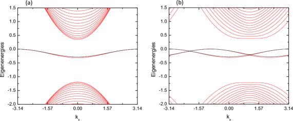
Figure 5: (Color online) The low energy spectrum of the phosphorene zig-zag nanoribbon. The degeneracy lifting of the quasi-flat band induced by the magnetic field can be noticed by comparing the two panels : in the left panel the magnetic flux is zero, while in the right panel $\Phi=0.01\Phi_{0}$. The red lines represent the numerically calculated spectrum for the width $M=71$, the black lines represent the analytical results Eq. (17) and Eq.(18).

In what follows, we turn our attention to the contribution to the spectrum coming from the Hamiltonian $H^{4}(k)$ in the presence of the magnetic field $\mathcal{B}$. As already mentioned, the case $B=0$ was studied perturbatively in Ezawa , where one proves that $t_{4}\neq 0$ generates the dispersion of the band, which thus becomes quasi-flat. In our calculation, we shall consider a large M and neglect the splitting $\delta$ (which is anyhow much smaller than the band dispersion). Then, the eigenvalues in the presence of the hopping $t_{4}$ and of the magnetic field $\mathcal{B}\neq 0$ will be given by the equation:

$$\begin{vmatrix}E-<\Psi_{A}|H^{4}|\Psi_{A}>&<\Psi_{A}|H^{4}|\Psi_{B}>\\ <\Psi_{B}|H^{4}|\Psi_{A}>&E-<\Psi_{B}|H^{4}|\Psi_{B}>\\ \end{vmatrix}=0.$$ (15)

Since $<\Psi_{A}|H^{4}|\Psi_{B}>=0$ the result reads:

$$E^{1}(k)=<\Psi_{A}(k)|H^{4}|\Psi_{A}(k)>=\sum_{m=1}^{M}\overline{t_{4A}}(m)\xi^{A*}_{k,m+1}\xi^{A}_{k,m}+c.c.$$

$$E^{2}(k)=<\Psi_{B}(k)|H^{4}|\Psi_{B}(k)>=\sum_{m=1}^{M}\overline{t_{4B}}(m)\xi^{B*}_{k,m+1}\xi^{B}_{k,m}+c.c.,$$ (16)

with the notation $\overline{t}_{4A}(m)=t_{4}\big{(}e^{i\phi_{4A}(m)}+e^{-i(\phi_{4A}(m)-k)}\big{)}$, and a similar one for $\overline{t}_{4B}(m)$.

For zero magnetic flux, in the limit $M\rightarrow\infty$, Eq.(16) yields Ezawa’s result:

$$E^{1}(k)=E^{2}(k)=-4\frac{t_{4}t_{1}}{t_{2}}(1+cosk),$$ (17)

saying that the levels remain degenerate but depend on $k$, such that they get a dispersion equal to $8t_{4}t_{1}/t_{2}$. However, the interesting case occurs at $\Phi\neq 0$ when the degeneracy is lifted. The exact summation in Eq.(16) is difficult, so we approximate it by taking advantage of the strong localization of the coefficients $\xi_{k1}^{A}$ and $\xi_{kM}^{B}$ at the edges $m=1$ and $m=M$, respectively. Using also Eq.(13) one obtains:

$$E^{1}(k,\Phi) \cong \overline{t}_{4A}(1,\Phi)\big{(}-\frac{\overline{t_{1}(1)}^{*}}{t_{2}}\big{)}|\xi^{A}_{k,1}|^{2}+c.c.$$

$$E^{2}(k,\Phi) \cong \overline{t}_{4B}(M-1,\Phi)\big{(}-\frac{\overline{t_{1}(M)}}{t_{2}}\big{)}|\xi^{B}_{k,M}|^{2}+c.c.~{},$$ (18)

with $E^{1}(k,\Phi)\neq E^{2}(k,\Phi)$, indicating the degeneracy lifting due to the magnetic field.

Figure 5 compares the quasi-flat spectrum in the absence (left panel) and presence (right panel) of the magnetic field applied on the ribbon. While the hopping $t_{4}$ generates the dispersion, the magnetic field gives rise to the degeneracy lifting. The red lines represent the numerical result, who considers all hopping parameters $t_{1},..,t_{5}$, while the black lines represent the analytical formulas Eq.(17) and Eq.(18) NoteEq18 calculated with $t_{3}=t_{5}=0$. The fit being very good, one concludes that the hopping parameters $t_{3}$ and $t_{5}$ have negligible influence on the spectrum, at least in the energy range of the quasi-flat band.

IV Quantum transport and superradiance in phosphorene mesoscopic plaquette

In order to investigate the transport properties in strong perpendicular magnetic field, we simulate the electronic Hall device by attaching four leads to a finite phosphorene plaquette (two leads for injecting/collecting the current, and two voltage probes), all the leads being contacted on the same zig-zag edge of the plaquette. The choice of such a lead configuration is essential, since it is the only one that can read out the current carried by the topological states located close to, and along the zig-zag edge. The electron transmission coefficients between different leads, the longitudinal, and the transverse resistance will be calculated as function of a gate potential $V_{gate}$ (at a given Fermi energy in the leads) in the Landauer-Büttiker formalism in terms of Green functions.

Depending on the position of the gate potential, different types of states become active in the transport process. Fig.3 shows the Hofstadter-type spectrum of the phosphorene plaquette composed of two unequal butterflies, corresponding to the conductance and valence band. As usual, the Landau levels accommodate bulk states, while the gaps that separate consecutive LL are filled with chiral edge states, induced by the quantizing magnetic field, and running all around the plaquette perimeter. One may observe in Fig.3 that the chirality $dE/d\Phi$ of the edge states is opposite in the two bands, fact that causes the different sign of the quantum Hall effect in the corresponding energy ranges.

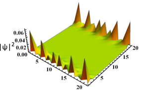
Figure 6: $|\Psi|^{2}$ for a pair of quasi-degenerate edge states of a finite- size plaquette in perpendicular magnetic field. The number of lattice sites is $21\times 20$, and the magnetic flux is $\Phi=0.1\Phi_{0}$.

One has to remark the presence in the semiconducting gap of a narrow, practically dispersionless band that accommodates also edge states, but of topological origin. They lie along the zig-zag edges only, exist also at $\mathcal{B}=0$, being the analogous of the edge states in the zig-zag ribbon discussed in the previous Section. It is important to underline that they do not get closed even if the magnetic field is applied, looking as in Fig.6. Figure 6 shows the superposition of two quasi-degenerate edge states located near the two (left and right) zig-zag boundaries. Any perturbation (as a small staggering $E_{A}\neq E_{B}$, impurity disorder or coupling to leads) lifts the superposition, and the wave functions become localized either on the left or right edge.

Two other striking features of the topological edge states on the plaquette will be proved here: i) the dissipative character, and ii) the splitting of the density of states, and the formation of minibands if the finite system is opened by attaching contacts; this behavior can be interpreted as a superradiance effect.

IV.1 The effective Hamiltonian and transport formalism

In order to calculate the transport quantities (namely, the longitudinal and transverse resistance) one needs to attach four leads to the finite-size plaquette. Then, the Hamiltonian of the entire system reads:

$$\mathcal{H}=H^{S}+H^{L}+\tau H^{LS},$$ (19)

where the first term is the Hamiltonian (2) of the phosphorene plaquette, the second term represents all the four semi-infinite leads (also in the tight-binding description), and the last one describes the coupling between the plaquette and the leads. The longitudinal and Hall resistances will be calculated as function of a gate potential $V_{gate}$ applied on the plaquette, similar to the experimental measurement, where $V_{gate}$ is simulated by a diagonal term in the Hamiltonian $H^{S}$.

A powerful tool to deal with such an open system is the formalism of the effective Hamiltonian, which is obtained by removing the degree of freedom of the leads, with the price of losing the Hermicity:

$$H^{S}_{eff}=H^{S}+\frac{\tau^{2}}{t_{L}}~{}e^{-ik}\sum_{\alpha}|\alpha\rangle\langle\alpha|~{},$$ (20)

where $t_{L}$ is the hopping parameter of the tight-binding model for the leads, $k$ parametrizes the energy in the leads, $E=2t_{L}cosk$, and $\{|\alpha\rangle\}$ are those localized states that correspond to the sites on the plaquette where the leads are sticked to the sample Note-lead . The difference between Hamiltonians Eq.(19) and Eq.(20) is just formal, and they are completely equivalent. The deduction of the effective Hamiltonian can be found for instance in Ref.6.

After constructing the matrix of the effective Hamiltonian in the representation of the localized functions $\{|nm\rangle\}$, one may calculate immediately the Green function $G(E)=(E-H_{eff}^{S})^{-1}$, which enters the Landauer-Büttiker formula for the transmission coefficients:

$$T_{\alpha\beta}=4\tau^{4}|G_{\alpha\beta}|^{2}Img^{L}_{\alpha}Img^{L}_{\beta}~{},~{}~{}~{}~{}\alpha\neq\beta~{},$$ (21)

where $\alpha$ and $\beta$ ($\alpha,\beta=1,..,4$) are lead indexes, and Im $g^{L}_{\alpha}$ represents the density of states in the lead $\alpha$. The transmission coefficients $T_{\alpha\beta}$ being known, the conductance matrix $g_{\alpha\beta}$, which connects all the currents $I_{\alpha}$ passing through the system to the corresponding voltages $V_{\beta}$, $I_{\alpha}=\sum_{\beta}g_{\alpha\beta}V_{\beta}$, can be obtained as $g_{\alpha\beta}=(e^{2}/h)T_{\alpha\beta}$ for $\alpha\neq\beta$, while the diagonal conductance $g_{\alpha\alpha}$ results from the current conservation rule $\sum_{\alpha}g_{\alpha\beta}=0$. Finally, the Landauer-Büttiker formalism provides the following expressions for the quantities of interest (longitudinal and Hall resistance), which are to be calculated numerically:

$$R_{L} = R_{14,23}=(g_{24}g_{31}-g_{21}g_{34})/|D|,$$

$$R_{H} = (R_{13,24}-R_{24,13})/2=(g_{23}g_{41}-g_{21}g_{43}-g_{32}g_{14}+g_{12}g_{34})/2|D|,$$ (22)

where D is any $3\times 3$ subdeterminant of the conductance matrix. Since the experimental curves show the conductance instead of the resistance, we shall do the same, and show in Fig.8 the the Hall and longitudinal conductance calculated as $G_{H}=R_{H}/(R_{H}^{2}+R_{L}^{2})$ and $G_{L}=R_{L}/(R_{H}^{2}+R_{L}^{2})$.

Figure 7: The sketch of a four-lead Hall device. All leads are connected to the same zig-zag edge.

IV.2 Quantum Hall effect in phosphorene

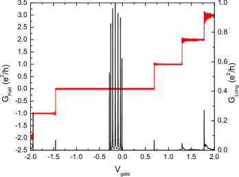
Figure 8: (Color online) Numerically calculated Hall (red line) and longitudinal (black line) conductance in the quantum Hall regime as a function of the gate potential $V_{gate}$, for a slightly disordered sample. The longitudinal conductance shows a series of peaks in the range of the quasi-flat band. The number of lattice sites is $107\times 40$, the magnetic flux is $\phi/\phi_{0}=0.1$, and the Fermi energy in the leads is $E_{F}=0$.

In what concerns the Hall conductance in the quantum regime, there are significant new aspects in comparison with the graphene. First, one has to notice the large plateau $G_{H}=0$ that corresponds to the central gap. Next, one notice the lack of the valley degeneracy in the low energy range, such that the quantum Hall plateaus are the conventional (spinless) plateaus $n=\pm 1,\pm 2,..$ in units $e^{2}/h$, the same as for the two-dimensional electron gas (2DEG) subject to a perpendicular magnetic field. As a specific feature, one may notice in Fig.8 that the lengths of the plateaus in the positive and negative regions are slightly different, as a manifestation of the spectral asymmetry discussed in Sec.II.

The quantum plateaus are supported obviously by the chiral edge states existing in the Hofstadter spectrum of the finite-size plaquette, however one should not forget that the central gap contains also topological edge states bunched in the quasi-flat band. The value $G_{H}=0$ everywhere in the gap confirms that these edge states are non-chiral, and do not support the QHE. Recall that, in terms of transmission coefficients, the chirality means $T_{\alpha,\alpha+1}=integer$, while $T_{\alpha,\alpha+1}=0$ (for any lead $\alpha$ and given direction of the magnetic field). On the other hand, in the spectral range occupied by the quasi-flat band, we find the symmetry $T_{\alpha,\alpha+1}=T_{\alpha,\alpha+1}$, which denotes the lack of chirality. This property was observed numerically using Eq.(21), and occurs no matter the presence or absence of the magnetic field.

The longitudinal conductance $G_{L}$ exhibits the non-dissipative behavior in the range of the quantum plateaus, as it should, but striking non-trivial properties are proved in the range [-0.3,0] covered by the quasi-flat band, where the longitudinal conductance is non-vanishing and shows a sequence of peaks. While the dissipative character of the non-chiral edges states was also met in the context of the zero-energy Landau level in graphene Levitov1 , we think that the peaked structure of the longitudinal conductance is specific to phosphorene.

It is already known that that the flat bands are sensitive to disorder due to their degeneracy Nita ; Leykam , and one may expect that the $G_{L}$ peaks are also affected by the disorder existing in the system, which is unavoidable experimentally. Indeed, the unitary limit $G_{L}=1e^{2}/h$ is reached only in the clean systems (this case is shown in Fig.9a), but any small amount of disorder allows for the backscattering and slightly lowers the values of the peaks below the unitary limit. This is the case in Fig.8, where small Anderson (diagonal) disorder was introduced in the numerical calculation.

In what follows we shall pay closer attention to properties of the non-chiral edge states in the quasi-flat band.

IV.3 Spectral and transport properties of the quasi-flat band in open system

It is obvious that the second term of the effective Hamiltonian Eq.(20) produces shifts of the real eigenvalues of $H^{S}$, but adds also an imaginary part, meaning the level broadening due to the coupling to the leads. As long as the coupling $\tau$ is very small (i.e., we are in the resonant tunneling regime, which was studied for the nanoribbon system in Schulz ), all the eigenvalues of $H^{S}$ should be practically recovered. However, with increasing coupling, the level broadening $\Gamma$ increases too, and the merging of neighboring levels occurs. Consequently, the shape of the density of states changes significantly. When $\Gamma\sim\Delta$ ($\Delta$ = mean interlevel distance) one enters the regime known as superradiative Zelevinsky . As we already mentioned the superradiance phenomenon consists in the overlapping and segregation of eigenenergies occurring in open systems under the control of the coupling between the finite system and the infinite reservoir. One may expect that the energy spectrum is not everywhere equally sensitive to this effect, and one may speculate that the energy range occupied by the states located near edges (where the leads are attached) is mostly affected.

We assume that the superradiance is the mechanism that gives rise to the miniband structure of the quasi-flat band shown in Fig.9a, where the density of states ($DOS=-\frac{1}{\pi}TrG$) exhibits eleven peaks. The confirmation comes from the calculation of the complex eigenvalues of the effective Hamiltonian (20). In Fig.9b we show the real and imaginary part of the eigenvalues in the energy range of the quasi-flat band, and find the presence of eleven energies with large imaginary part, which perfectly correspond to the positions of the minibands in the density of states. One has to observe in Fig.9b also the multitude of eigenstates with vanishing imaginary part ($ImE=0$). They correspond to the edge states localized along the edge opposite to that one where the leads are connected. In other words, the process of overlapping and segregation affects only those edge states that are in the immediate vicinity of the leads, the other ones remaining unchanged.

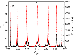
Figure 9: (Color online) (a) The peaked structure of the transmission coefficient $T_{12}$ (red line) and the density of states (black line) of the phosphorene plaquette in the energy range of the quasi-flat band for a clean system. Note that not all the DOS peaks are transmitting, and also that the unitary limit of the transmission is reached. (b) $ImE$ vs $ReE$ for the eigenvalues of the effective Hamiltonian (20) corresponding to the quasi-flat band. Note that the eigenvalues with $ImE\neq 0$ correspond to the miniband structure in the panel (a). The number of lattice sites is $107\times 40$, the magnetic flux is $\Phi=0.1\Phi_{0}$, the Fermi energy in the leads is $E_{F}=0$, and $\tau=2eV$.

As a next step, we draw the attention to the fact, visible in Fig.9a, that not all DOS peaks support the electron transmission. This apparently surprising result has a simple explanation in terms of the charge distribution on the plaquette, described by the local density of states. The local density of states, calculated at each site $i$ on the plaquette as the imaginary part of the Green function $LDOS_{i}(E)=-\frac{1}{\pi}ImG_{ii}(E)$, shows that, in the case of the conducting minibands, the states are located between the contacts, but, for the non-conducting ones, the states are positioned outside the contacts. The two situations are displayed in Fig.10, The same figure tells furthermore that the states accommodated by the minibands do not get closed around the whole perimeter of the plaquette, even at such strong magnetic fields that generates chiral edge states in the bands.

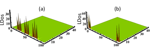
Figure 10: (Color online): The local density of states (LDOS) in the presence of the leads: (a) the density of states is localized in-between the leads and contribute to transmission (corresponding to the peak at $V_{gate}=-0.0978eV$ in Fig.9a), and (b) the density of states is localized outside the leads and corresponds to the non-transmitting DOS peak at $V_{gate}=-0.10735eV$ in Fig.9a. The parameters are the same as in Fig.9.

In what concerns the transport properties, besides the lack of chirality mentioned above, we find that the transmission exhibits a peaked structure and reaches the unitary limit $T_{\alpha\alpha+1}=T_{\alpha+1\alpha}=1$ in the middle of the conducting minibands. This behavior of the transmission coefficients is proved by numerical investigation using Eq.(21), and it is shown in Fig.9a. (Of course, the unitary limit, telling that each miniband behaves as a perfect one-dimensional channel, is reached only for disorder-free systems.) All the other transmission coefficients vanish, so that the whole $4\times 4$ conductance matrix reads as:

$$\text{{\bf g}}=\frac{e^{2}}{h}\begin{pmatrix}-1&~{}1&0&0\\ ~{}1&-2&1&0\\ 0&1&-2&1\\ 0&0&1&-1\end{pmatrix},$$ (23)

and allows for the calculation of the Hall ($R_{H}$) and longitudinal ($R_{L}$) resistances. Indeed, by the use of Eq.(22), one obtains the results already known from the numerical calculation. For the Hall resistance one gets $R_{H}=0$, which is the outcome of the lack of chirality, however, a non-trivial result is obtained for the longitudinal response, for which the above matrix yields $R_{L}=1h/e^{2}$, indicating a dissipative character of the electron transport in minibands. It is to underline that this distinctive property of the quasi-flat band occurs even in the presence of a strong magnetic field, which, otherwise, is able to generate in the other bands the specific QHE behavior, i.e., quantized non-zero values of $R_{H}$, and non-dissipative $R_{L}$.

V summary and conclusions

In this paper we have studied spectral and transport properties of phosphorene, paying special attention to confined systems (zig-zag ribbon and mesoscopic plaquette) subject to a magnetic field, with main focus on the topological edge states organized in the quasi-flat band. Our results are the following:

We approach analytically the question of electron-hole symmetry breaking, and demonstrate the role played in this respect by the hopping integral $t_{4}$, the only parameter in the tight-binding model that violates the bipartitism of the lattice.

The Hofstadter-type spectrum of the phosphorene plaquette misses the usual periodicity $E(\Phi)=E(\Phi+\Phi_{0})$ because three different Peierls phases (depending also on the quasi-2D lattice angle $\beta$) are assigned to different hopping terms. The Hofstadter spectrum comprises edge states of chiral and topological origin. The chiral states fill the gaps between the Landau levels and extend all around the perimeter. The other ones extend along the zig-zag edges only, and remain like that even in strong magnetic field. The topological states are bunched in a quasi-flat band located in the middle of the gap.

For the zig-zag ribbon, since $|t_{1}/t_{2}|<1$, we prove that the topological edge states occur at any momentum $k$ in the Brillouin zone, contrary to the graphene case. We analytically show that the degeneracy of a pair of edge states, located at opposite edges of the ribbon, occurs only in the limit of the infinite wide ribbon ($M\rightarrow\infty$), and we prove also that the degeneracy is lifted by the magnetic field.

The quantum transport in the mesoscopic plaquette is treated numerically. The Hall device may use different lead configuration, however the configuration ’all leads on the same edge’ (Fig.7) is that one that evidence better the features of the edge states. We suggest such a configuration for an eventual experimental study of the topological edge states. Specific to phosphorene, the Hall conductance shows a zero plateau in the gap, indicating the non-chiral behavior of the quasi-flat band, but a non-zero longitudinal conductance, indicating the dissipative character. The multiple-peak aspect of $G_{L}$ reflects the miniband structure of the density of states in the presence of the leads.

For the energy range occupied by the quasi-flat band, we calculate the transmission coefficient between consecutive leads, the DOS of the plaquette when connected to the leads, and the complex eigenenergies of the non-Hermitian effective Hamiltonian. The ensemble of these quantities (shown in Fig.9), which are controlled by the dot-lead coupling parameter $\tau$, certifies the manifestation of the superradiance phenomenon in phosphorene. We underline that not all the minibands in the DOS are conducting (Fig.9a), the issue being explained by Fig.10. We mention the features of the electron transmission, which besides the lack of chirality, exhibits unitary peaks in the case of the clean system, proving a one-channel- type transport.

In what concerns the disorder effects, it is clear that the different quantum states respond differently to disorder. While the chiral states are robust, one expects the topological edge states be sensitive due to their quasi-degeneracy. We think that the localization, level spacing analysis, and the electron transmission are topics of interest, which are however beyond the aim of this paper.

In conclusion, phosphorene is a ’beyond’ graphene material which, besides potential applications as a semiconductor, shows several interesting conceptual properties, mainly concerning the topological edge states accommodated in the quasi-flat band.

VI Acknowledgments

We are grateful to Antonio Castro Neto for illuminating discussions on the phosphorene issue, and to Marian Nita for helpful comments. We acknowledge financial support from PNII-ID-PCE Research Programme (grant no 0091/2011) and Romanian Core Research Programme.

References

- (1) A. N. Rudenko and M. I. Katsnelson, Phys. Rev. B 89, 201408(R) (2014).
- (2) G. Montambaux, F. Pie´chon, J.-N. Fuchs, and M. O. Goerbig, Phys. Rev. B 80, 153412 (2009).
- (3) M.O. Goerbig, Rev. Mod.Phys. 83, 1193 (2011).
- (4) A.Mielke, Phys.Lett. A 174, 443 (1993).
- (5) M. Ezawa, New J. Phys. 16,115004 (2014).
- (6) V. Moldoveanu, A. Aldea, A. Manolescu, and M. Nita, Phys. Rev. B 63, 045301 (2000).
- (7) N. Hatano and D. R. Nelson, Phys.Rev.Lett. 77, 570 (1996).
- (8) I. Ya. Goldsheid and B. A. Khoruzhenko, Phys. Rev. Lett. 80, 2897 (1998).
- (9) G. L. Celardo and L. Kaplan, Phys. Rev. B 79, 155108 (2009).
- (10) A. I. Nesterov, F. Aceves de la Cruz, V. A. Luchnikov, and G. Berman, Phys. Lett. A 379, 2951 (2015).
- (11) X. Y. Zhou, R. Zhang, J. P. Sun, Y. L. Zou, D. Zhang, W. K. Lou, F. Cheng, G. H. Zhou, F. Zhai, and K. Chang, Scientific Reports 5,12295 (2015).
- (12) L. Li, F. Yang, G. J. Ye, Z. Zhang, Z. Zhu, W. K. Lou, L. Li, K. Watanabe, T. Taniguchi, K. Chang, Y. Wang, X.H. Chen, and Y. Zhang, arXiv:1504.07155 [cond-mat.mes-hall].
- (13) L. Li, G. J. Ye, V. Tran, R. Fei, G. Chen, H. Wang, J. Wang, T. Taniguchi, Li Yang, X. H. Chen, and Y. Zhang, Nature Nanotechnol. 10, 608 (2015).
- (14) H. Liu, A. T. Neal, Z. Zhu, Z. Luo, X. Xu, D. Tománek, and P. D. Ye, ACS Nano 8, 4033 (2014).
- (15) A. Mishchenko, Y. Cao, G. Yu, C. R. Woods, R. V. Gorbachev, K. S. Novoselov, A. K. Geim, and L. Levitov, Nano Lett. 15, 6991 (2015).
- (16) A. S. Rodin, A. Carvalho, and A. H. Castro Neto, Phys. Rev. Lett. 112, 176801 (2014).
- (17) R. Fei and L. Yang, Nano Lett. 14, 2884 (2014).
- (18) Q. Wu, L. Shen, M. Yang, Y. Cai, Z. Huang, and Y. P. Feng, Phys. Rev. B 92, 035436 (2015).
- (19) L. Li, Y. Yu, G. J. Ye, Q. Ge, X. Ou, H. Wu, D. Feng, X. H. Chen, and Y. Zhang, Nature Nanotechnol. 9 , 372 (2014).
- (20) The particular expression of the phases depend on the choice of the origin; in our case they correspond to the choice in Fig.1
- (21) J. M. Pereira Jr. and M. I. Katsnelson, Phys. Rev. B 92, 075437 (2015).
- (22) Motohiko Ezawa, Journal of Physics: Conference Series 603, 012006 (2015).
- (23) R. Zhang, X.Y. Zhou, D. Zhang, W. K. Lou, F. Zhai, K. Chang, arXiv:1507.03808 [cond-mat.mes-hall]
- (24) E. Taghizadeh Sisakht, M. H. Zare, and F. Fazileh, Phys. Rev. B 91,085409 (2015).
- (25) A.Carvalho, A. S. Rodin and A.H. Castro Neto, EPL, 108, 47005 (2014).
- (26) K. Wakabayashi, M. Fujita, H. Ajiki, and M. Sigrist, Phys. Rev. B 59, 8271 (1999).
- (27) We remind that in the graphene ribbon, since , the convergence, and, consequently, the flat band occur only for comprised between the points and in the Brillouin zone Wakabayashi .
- (28) In Fig.5(right), the black lines represent Eq.(18), where has been considered.
- (29) One has to keep in mind the technical detail that each lead is composed of several one-dimensional independent channels, and that in Eq.(20) the summation over all the channels is implicit. The same convention is assumed also in Eq.(21).
- (30) D. A. Abanin, K. S. Novoselov, U. Zeitler, P. A. Lee, A. K. Geim, and L. S. Levitov, Phys. Rev. Lett. 98, 196806 (2007).
- (31) M. Nita, B. Ostahie, and A. Aldea, Phys. Rev. B 87, 125428 (2013).
- (32) D. Leykam, S. Flach, O. Bahat-Treidel, and A. S. Desyatnikov, Phys. Rev. B 88, 224203 (2013).
- (33) J. Paez, D. A. Bahamon, Ana L. C. Pereira, and P. A. Schulz, arXiv:1506.03093 [cond-mat.mes-hall].
- (34) A. Ziletti, F. Borgonovi, G. L. Celardo, F. M. Izrailev, L. Kaplan, and V. G. Zelevinsky, Phys. Rev. B 85, 052201 (2012).