Capillary Wave Theory of Adsorbed Liquid Films and the Structure of the Liquid-Vapor Interface

Abstract

In this paper we try to work out in detail the implications of a microscopic theory for capillary waves under the assumption that the density is given along lines normal to the interface. Within this approximation, which may be justified in terms of symmetry arguments, the Fisk-Widom scaling of the density profile holds for frozen realizations of the interface profile. Upon thermal averaging of capillary wave fluctuations, the resulting density profile yields results consistent with renormalization group calculations in the one loop approximation. The thermal average over capillary waves may be expressed in terms of a modified convolution approximation where normals to the interface are Gaussian distributed. In the absence of an external field we show that the phenomenological density profile applied into the square gradient free energy functional recovers the capillary wave Hamiltonian exactly. We extend the theory to the case of liquid films adsorbed on a substrate. For systems with short range forces, we recover an effective interface Hamiltonian with a film height dependent surface tension that stems from the distortion of the liquid-vapor interface by the substrate, in agreement with the Fisher-Jin theory of short range wetting. In the presence of long range interactions, the surface tension picks up an explicit dependence on the external field and recovers the wave-vector dependent logarithmic contribution observed by Napiorkowski and Dietrich. Using an error function for the intrinsic density profile, we obtain closed expressions for the surface tension and the interface width. We show the external field contribution to the surface tension may be given in terms of the film’s disjoining pressure. From literature values of the Hamaker constant, it is found that the fluid-substrate forces may be able to double the surface tension for films in the nanometer range. The film height dependence of the surface tension described here is in full agreement with results of the capillary wave spectrum obtained recently in computer simulations, and the predicted translation mode of surface fluctuations reproduces to linear order in field strength the exact solution of the density correlation function for the Landau-Ginzburg-Wilson Hamiltonian in an external field.

I Introduction

The structure of the liquid-vapor interface and the corresponding capillary wave fluctuations continue to receive a great deal of attention after many decades of research.Höfling and Dietrich (2015); Parry, Rascón, and Evans (2015); Chacón and Tarazona (2016) Under the mean field approximation, the statistical mechanics of interfaces is most conveniently expressed in terms of Density Functional Theory.Evans (1979, 1992) This approach provides an intrinsic density profile, which only depends on molecular details of the fluid under study. A wide-reaching implication is the Fisk-Widom scaling hypothesis, which suggests that close to the critical point the density profile becomes universal.Fisk and Widom (1969); Rowlinson and Widom (1982) However, already within the mean field approximation, a more detailed study of density correlations indicates that liquid-vapor interfaces exhibit a long wavelength instability, whence, divergent fluctuations in the thermodynamic limit (however far from the bulk critical point).Zittartz (1967); Jasnow and Rudnick (1978); Evans and Wilding (2015); Parry, Rascón, and Evans (2015) This situation implies that an accurate description of the interface must be carried out within the framework of renormalization group theory. Explicit calculations for simple models show that the correct averaged density includes the mean field intrinsic density profile as leading order contribution. However, to second order a new term appears which does not conform to the Fisk-Widom scaling, but is rather, extrinsic, i.e., it depends also on the system size, at least on scales smaller than the parallel correlation length, $\xi_{\parallel}$ that is of macroscopic range for a fluid interface under gravity.Jasnow and Rudnick (1978); Abraham (1981); Jasnow (1984); Köpf and Münster (2008); Delfino and Viti (2012)

A far more intuitive approach to the study of interface fluctuations may be achieved in terms of capillary wave theory.Buff, Lovett, and Stillinger (1965); Weeks (1977); Bedeaux and Weeks (1985) Here, one assumes that surface fluctuations may be singled out from bulk fluctuations by performing a pre-average on the length-scale of the bulk correlation length.Weeks (1977); Huse, van Saarloos, and Weeks (1985) The properties of the undulated film profile that results may be then studied analytically, and it is found that the origin of the diverging structure factor may be traced to capillary wave fluctuations of the interface.Jasnow and Rudnick (1978); Evans and Wilding (2015); Parry, Rascón, and Evans (2015) The thermal average of such fluctuations provides an extrinsic interface width that is proportional to $\ln\xi_{\parallel}$, in agreement with renormalization group theory and exact calculations.Jasnow and Rudnick (1978); Abraham (1981); Fisher, Fisher, and Weeks (1982); Köpf and Münster (2008)

X-ray scattering experiments as well as computer simulations have confirmed the predictions of renormalization group and capillary wave theories, but also indicate that the divergence of fluctuations is in practice a minor concern for typical macroscopic samples.Braslau et al. (1988); Ocko et al. (1994); Doerr et al. (1999); Benjamin (1992); Müller and Schick (1996); Lacasse, Grest, and Levine (1998); Vink, Horbach, and Binder (2005)

Be as it may, the presence of an extrinsic interface width indicates an important conceptual limitation of the usual mean field approach. For this reason, efforts have been devoted to incorporate the parallel interface fluctuations within density functional theory and to account for capillary wave fluctuations at the microscopic level.Davis (1977); Napiórkowski and Dietrich (1993); Robledo and Varea (1997); Mecke and Dietrich (1999); Stecki (2001); Blokhuis (2009) Particularly, recent studies have emphasized the need to account for the interface curvature, and indicate that it is possible to recover an effective capillary wave Hamiltonian from fully microscopic functionals, provided one considers an extended wave-vector dependent surface tension.Mecke and Dietrich (1999); Blokhuis (2009) Unfortunately, it has also been argued convincingly that it is not possible to determine unambiguously these wave-vector dependent corrections to the surface tension from x-ray scattering experiments.Paulus, Gutt, and Tolan (2008); Pershan and Schlossman (2012); Parry, Rascón, and Evans (2015) The reason is that surface and bulk fluctuations entangle at the large wave-vectors that would be required to measure such corrections. Whence, the only way to study interface fluctuations at small length-scales is adopting an arbitrary but consistent prescription for the interface location and measuring its fluctuations by means of computer simulations.Chacon and Tarazona (2003, 2005); Tarazona, Checa, and Chacon (2007)

An apparently unrelated issue is the study of short range wetting, i.e., the transition that takes place when the only driving force to wetting is a very short range attractive interaction of the fluid to the substrate.Parry and Rascón (2009); Bryk and Binder (2013) In this limit, as the film thickens the liquid-vapor interface fluctuations become large, and are akin to the usual capillary wave fluctuations of a free interface. Theoretical studies on this topic indicate that the substrate distorts the liquid-vapor profile,Jin and Fisher (1993); Parry et al. (2006) and therefore conveys a film height dependence to the surface tension (also known as position dependent stiffness) of which there are currently strong indications from computer simulations.Fernández, Chacón, and Tarazona (2012); Fernández et al. (2015)

Recently, we studied the interface fluctuations of an adsorbed film in the presence of a long range external field.MacDowell, Benet, and Katcho (2013); MacDowell et al. (2014); Benet et al. (2014) In this case, the liquid-vapor interface feels the substrate directly via the long range forces, rather than indirectly, via weak substrate-fluid correlations. As a result, the surface tension picks up a strong film height dependence, which increases with the intensity and range of the external field.Bernardino et al. (2009) Indications of this effect observed already some time agoWerner et al. (1999) have been confirmed by a number of recent simulations, which show that the film height dependence may be related to the film’s disjoining pressure.MacDowell, Benet, and Katcho (2013); MacDowell et al. (2014); Benet et al. (2014)

Already a while ago, Davis suggested that a microscopic explanation of capillary waves may be achieved by assuming the density is given in terms of the perpendicular distance to the interface position.Davis (1977) This idea, which looks quite intuitive and may be justified from microscopic free energy functionals,Diehl, Kroll, and Wagner (1980); Kawasaki and Ohta (1982); Huse, van Saarloos, and Weeks (1985) has been henceforth explored in depth.Mecke and Dietrich (1999); Stecki (2001); Blokhuis (2009) However, it appears that some of its implications may have been overlooked. In a recent paper, we showed that in fact it is able to explain accurately the interface fluctuations in the presence of long range external fields, and particularly, the relation of the surface tension with the disjoining pressure.Benet et al. (2014) A more direct test of this hypothesis may be obtained from calculations of density profiles of absorbed films.Nold et al. (2014); Hughes, Thiele, and Archer (2015); Nold et al. (2015) Particularly, accurate density functional calculations of the density profile in the vicinity of the three phase contact line (i.e., the rim of sessile droplets) by Nold et al. have confirmed that the hypothesis is valid for adsorbed films even a few molecular diameters away from the substrate.Nold et al. (2016)

In this paper we try to work out in detail the implications of a microscopic theory for capillary waves under the assumption that the density is given along lines normal to the interface.Davis (1977) Our study provides interface Hamiltonians for adsorbed films in a variety of systems, and shows that the corrections to the classical capillary wave spectrum are of the same order as the surface tension. Whereas it seems difficult to disentangle the signature of such corrections in surface scattering experiments, they seem to be in full agreement with recent computer simulations.MacDowell, Benet, and Katcho (2013); MacDowell et al. (2014); Benet et al. (2014) Interestingly, our study also sheds some light on the nature of the liquid-vapor interface in the absence of external fields and allows us to reconcile the Fisk-Widom scaling hypothesis with capillary wave theory.

In the next section we make some general remarks that motivate the phenomenological approach that is adopted here. We then formalize the approximation and discuss its implications as regards the structure of the density profile (Sec. III). The study follows with the formulation of effective interface Hamiltonians for a variety of fluid-fluid and fluid-substrate interactions (Sec. IV), which are then applied for a simple intrinsic density profile with the shape of an error function (Sec V). Finally, in section VI we compare our predictions with exact solutions for the Landau-Ginzburg-Wilson Hamiltonian. Our findings are summarized in the conclusion.

II Preliminary Definitions

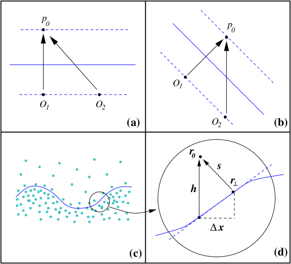
Figure 1: Sketch of simple model interfaces. (a) For a flat interface profile (full line), choosing a reference frame $O_{1}$ perpendicular to the interface, one finds isodensity lines (dashed) are given by the vertical distance $z-\ell$. (b) For an arbitrary reference frame, $O_{2}$, the interface appears tilted, and the isodensity lines depend simultaneously on $\mathbf{x}$ and $z$. (c) At a microscopic scale a smooth film profile may be defined after averaging at the scale of the correlation length. (d) At a scale (circle) that is smaller than the curvature of $\mathcal{L}$ but larger than the correlation length, the interface looks flat but tilted. The perpendicular distance from the film to a point $\mathbf{r}_{0}=(\mathbf{x}_{0},z_{0})$ may be determined approximately as a local function of $\mathbf{x}_{0}$.

II.1 Symmetry

Consider an atomic fluid in a state of vapor-liquid coexistence. A configuration of the system may be specified in terms of the instantaneous density $\hat{\rho}(\mathbf{r})$, as dictated by the set of atomic coordinates of the fluid. This density field is highly discontinuous, but a related continuous density $\rho(\mathbf{r})$ may be determined as a thermal average of $\hat{\rho}(\mathbf{r})$ on the scale of the correlation length. Having $\rho(\mathbf{r})$ at hand, it is possible to define an interface as the loci of points with a prescribed density laying between bulk liquid and vapor densities. Alternatively, from a given configuration, the interface location may be specified using a smooth density operator with width equal to the bulk correlation length,Willard and Chandler (2010) or by a suitable percoleation algorithm.Chacon and Tarazona (2005); Tarazona, Checa, and Chacon (2007) In either case, a hypothetical situation may be envisaged where the thermal fluctuations of the interface position have been supressed. A point in space, $\mathbf{r}$, may be given in terms of $\mathbf{x}$ and $z$, where the latter is a direction perpendicular to the interface, and $\mathbf{x}$ is a vector perpendicular to $z$. Choosing a suitable dividing surface, the corresponding planar film profile, say $\pi$, located at position $z=\ell$, is completely flat and devoid of any roughness at all length scales beyond the bulk correlation length, as sketched in Fig.1.a. The density, $\rho(\mathbf{r})$, which will generally depend on $\mathbf{r}$ in this case is a single function of the distance $s$ away from the interface. This serves to define an intrinsic density profile $\rho_{\pi}(s)$, which is defined here as the mean field density profile obtained from the underlying microscopic free energy functional.

By virtue of rotational invariance, the density of a tilted interface, as in Fig.1.b will be still given by $\rho_{\pi}(s)$, but now $s$ will no longer be a single function of the vertical distance $z-\ell$, but will also depend on $\mathbf{x}$. Whence, in the absence of an external field, the only relevant direction in the hypothetical system of Fig.1.a-b is the perpendicular distance to the interface, and densities along that line are invariant to the choice of reference frame.Davis (1977); Zia (1985)

In practice, the length scale relevant for the action of an external fields is often much larger than the length scale of density correlations. Such is the case of a liquid–vapor interface, where the density profile decays in the length scale of a few angstrom, while the capillary length, which sets the scale of action of gravity, is of the order of the millimeter. Whence, the full density profile may be described perturbatively as that pertaining to a free interface, plus a small correction which will depend on the direction along the external field.

II.2 Non-locality

In practice, interfaces are not flat as in Fig.1.a, but rather, have a rough profile that results from thermal fluctuations (Fig.1.c). Consider now a hypothetical case were we could constrain a given realization of the film profile $\mathcal{L}(\mathbf{x})$, with average $\left\langle\mathcal{L}\right\rangle=\ell$. Clearly, the resulting constraint density profile $\rho(\mathbf{r};\mathcal{L})$, can no longer be expressed in terms of a single variable, but rather, depends on all three Cartesian coordinates $\mathbf{r}$ (Fig.1.c). Likewise, $\rho(\mathbf{r};\mathcal{L})$ can no longer be expressed in terms of the simple intrinsic density, but rather, must pick up a functional dependence of the full film profile, as indicated by the second argument $\mathcal{L}$ of $\rho(\mathbf{r};\mathcal{L})$. Fisher, Jin, and Parry (1994) Such must be the case when the film profile exhibits a finite local curvature, $1/R$, for the observer locally will not be able to tell whether that curvature corresponds to a fraction of a droplet or bubble of radius R, or rather, to a piece of an undulated film profile Mecke and Dietrich (1999); Blokhuis (2009). Hence, the density in the vicinity of the curved film must conform to the Laplace equation and deviate from the resulting planar interface. It is expected that such density distortions could be described by the Laplacian of the film profile, at least for small curvatures Safran (1994); Chaikin and Lubensky (1995).

If, however, the local radius of curvature is much larger than the bulk correlation length and we are interested in the density at a point $\mathbf{r}_{0}=(\mathbf{x}_{0},z_{0})$ a distances much smaller than $R$ away from the interface, the fluid feels locally a tilted film with no curvature (Fig.1.d). Following the arguments of the previous section, the density along a line perpendicular to the film profile should then be approximately given in terms of $\rho_{\pi}$ and the single variable $s$, hence, as a local function of $s$.Davis (1977)

Let $\mathbf{r}_{\perp}=(\mathbf{x}_{\perp},\mathcal{L}(\mathbf{x}_{\perp}))$ be the point on $\mathcal{L}(\mathbf{x})$ that is closest to $\mathbf{r}_{0}$. The perpendicular distance of $\mathbf{r}_{0}$ to the film profile may then be given as $s^{2}=\Delta\mathbf{x}^{2}(1+m_{\perp})$, where $|\Delta\mathbf{x}|$ is the distance between points $\mathbf{x}_{\perp}$ and $\mathbf{x}_{0}$ on the plane perpendicular to the $z$ axis; while $m_{\perp}$ is the slope of a vector perpendicular to $\mathcal{L}$ at $\mathbf{r}_{\perp}$.

Clearly, the slope $m_{\perp}$ is a local property of $\mathcal{L}$ at point $\mathbf{r}_{\perp}$. If, however, one can describe $\mathcal{L}(\mathbf{x})$ at $\mathbf{x}_{\perp}$ in terms of a Taylor expansion about $\mathbf{x}_{0}$ with sufficient accuracy, then we can give $s$ fully as a local function of $\mathcal{L}$, $\nabla_{\mathbf{x}}\mathcal{L}$, $\nabla_{\mathbf{x}}^{2}\mathcal{L}$, etc. at $\mathbf{x}_{0}$. In this favorable case, we can then describe the density profile as $\rho_{\pi}(s)$, hence, also as an extended local function at $\mathbf{x}_{0}$ (Fig.1.d).

In the most general case, however, $\mathcal{L}(\mathbf{x})$ at an arbitrary point can not be given as a Taylor expansion at sufficient distances away from $\mathbf{x}_{0}$. Whence, the location of $\mathbf{x}_{\perp}$ and accordingly, the norm $|\Delta\mathbf{x}|$ will become a highly nonlocal property, which can only be determined if the full film profile is known all the way from $\mathbf{x}_{0}$ to $\mathbf{x}_{\perp}$.Mecke and Dietrich (1999) Furthermore, there could emerge several perpendicular distances to a given point, only one corresponding to the shortest distance to that point. As a result, even if the density profile $\rho(\mathbf{r};\mathcal{L})$ could be given in terms of the intrinsic density profile, the function $\rho_{\pi}(s)$ would become a highly nonlocal function.

The relevance of nonlocal effects on the density profile of rough interfaces has been emphasized at length by Parry and collaborators Parry et al. (2006, 2007); Bernardino et al. (2009); Parry and Rascón (2009). Such effects are particularly important in the study of short range critical wetting, where the external field is zero at all distances beyond the bulk correlation length.

In what follows, we will argue that for films subject to external fields of range greater than the bulk correlation length, an extended local approximation to the density profile is sufficient to capture the leading order corrections to the classical capillary wave theory.

The origin of the extended locality is introduced in the theory under the assumption that the density is a single variable of $s$. The observation that the density profile is best expressed as a function of the perpendicular distance to the interface has already been stressed previously Davis (1977); Diehl, Kroll, and Wagner (1980); Kawasaki and Ohta (1982); Zia (1985); Stecki (1998); Mecke and Dietrich (1999); Stecki (2001); Blokhuis (2009). In the next section we will show that for small deviations away from planarity, $s$ may be expressed easily in terms of a film profile and its gradient, and explore the consequences of this assumption.

III Density profile

In the classical theory of capillary fluctuations, the density of a rough instantaneous configuration at a point $\mathbf{r}$ is dictated merely by the vertical distance of that point from the film profile $\mathcal{L}(\mathbf{x}{})$. Accordingly, the density profile $\rho(\mathbf{r};\mathcal{L})$ may be expressed in terms of an assumed intrinsic density profile, $\rho_{\pi}(z)$ of the single variable $h(z,\mathbf{x}{})=z-\mathcal{L}(\mathbf{x}{})$, as:

$$\rho(\mathbf{r};\mathcal{L})=\rho_{\pi}(h(z,\mathbf{x}{}))$$ (1)

In the previous section, however, we argued that in the low curvature limit, the density at a point should depend on the perpendicular distance to the interface. Accordingly, the starting point of our study is to consider that we can describe the full density still in terms of a function of $\rho_{\pi}(z)$, but, with a more complex dependence given by the single variable $s(z,\mathbf{x}{})$. Whence, we will henceforth explore the implications of the following ansatz:

$$\rho(\mathbf{r};\mathcal{L})=\rho_{\pi}(s(z,\mathbf{x}{}))$$ (2)

As discussed above, this assumption will be accurate in the low curvature limit, where $s(z,\mathbf{x}{})$ is then a purely local function of $\mathcal{L}$ and $(\nabla_{\mathbf{x}}\mathcal{L})^{2}$,

$$s(z,\mathbf{x}{})=\frac{z-\mathcal{L}(\mathbf{x})}{\sqrt{1+(\nabla_{\mathbf{x}}\mathcal{L})^{2}}}$$ (3)

Eq. (2) together with Eq. (3) are the starting point of our theoretical approach. Clearly, if we neglect the gradient, Eq. (1) and Eq. (2) are equivalent and the only significant fluctuations are given by the interface displacements away from the average film profile $\delta\mathcal{L}(\mathbf{x})=\mathcal{L}(\mathbf{x})-\ell$, as in the classical theory Buff, Lovett, and Stillinger (1965); Weeks (1977).

In fact, it has been shown that Eq. (2) is a systematic low temperature solution of the Landau-Ginzburg-Wilson Hamiltonian for a rough interface.Diehl, Kroll, and Wagner (1980) Such statement holds exactly to zeroth order, provided one defines the film profile $\mathcal{L}$ as a collective coordinate obeying the condition:Diehl, Kroll, and Wagner (1980); Kawasaki and Ohta (1982); Huse, van Saarloos, and Weeks (1985)

$$\int\hat{\rho}(\mathbf{r})\frac{d\rho_{\pi}(z-\mathcal{L}(\mathbf{x}))}{dz}dz=0$$ (4)

As discussed recently, this definition of the film profile is closely related to microscopic definitions employed to locate $\mathcal{L}(\mathbf{x})$ in computer simulation experiments, and are close to the optimal choice required to extract the capillary wave signature from the spectrum of surface fluctuations.Hernández-Muñoz, Chacón, and Tarazona (2016)

III.1 Linearisation

Although the ansatz embodied in Eq. (2) allows us to remove the nonlocal character of the constraint density profile, the problem is far more complex than in the classical theory, since the variable $s$ can no longer be interpreted as a translation of the interface position. As a result, an expansion of $s$ about $z-\ell$ to quadratic order does not satisfy the condition $s(z,\mathbf{x})=0$ for $z=\mathcal{L}(\mathbf{x})$. Ignoring this limitation, it is still possible to expand $s$ to quadratic order in the interface fluctuations, and express it in terms of an effective translation about the average planar interface as considered previously by Stecki:Stecki (1998)

$$s(z,\mathbf{x}{})=h_{\pi}(z)-\delta s_{\pi}(z,\mathbf{x}{})$$ (5)

where:

$$\begin{array}[]{lll}h_{\pi}(z)&=&z-\ell\\ &&\\ \delta s_{\pi}(z,\mathbf{x}{})&=&\delta\mathcal{L}(\mathbf{x}{})+\frac{1}{2}h_{\pi}(z)(\nabla_{\mathbf{x}}\mathcal{L})^{2}\end{array}$$ (6)

Accordingly, we can assume that the full density profile is given in terms of effective translations, exactly as in the classical capillary wave theory; However, the translation is here along a direction perpendicular to the interface, rather than merely along the vertical direction:

$$\rho(\mathbf{r};\mathcal{L})=\rho_{\pi}(h_{\pi}-\delta s_{\pi}(z,\mathbf{x}{}))$$ (7)

This result resembles a related approach by van Leeuwen and Sengers, who hypothesized that the density profile could be given in terms of a compressed shift of the interface position, rather than by a mere translation, i.e., they assumed local displacements of the form $z-\alpha(z)\mathcal{L}$, with $\alpha(z)$ an undetermined compression factor which is evaluated a posteriori from thermodynamic considerations.Leeuwen and Sengers (1989) A similar strategy has been adopted by Robledo and Varea.Robledo and Varea (1997) In our approach, the compression factor is given directly in terms of the film profile gradient, and has a clear physical origin.

Having written the normal distance in terms of a linearized normal translation, we can now expand $\rho(\mathbf{r};\mathcal{L})$ in powers of $\delta s_{\pi}$ up to second order as:

$$\rho(\mathbf{r};\mathcal{L})=\rho_{\pi}(z;\ell)-\frac{d\rho_{\pi}(z;\ell)}{dz}\delta s_{\pi}(z,\mathbf{x}{})+\frac{1}{2}\frac{d^{2}\rho_{\pi}(z;\ell)}{dz^{2}}\delta s_{\pi}^{2}(z,\mathbf{x}{})$$ (8)

Since Eq. (5) is only accurate up to quadratic order in deviations about $\mathcal{L}=\ell$, we drop all higher order terms in the above result and are left with the following equation:

$$\rho(\mathbf{r};\mathcal{L})=\rho_{\pi}(z;\ell)-\frac{d\rho_{\pi}(z;\ell)}{dz}\delta\mathcal{L}(\mathbf{x}{})-\frac{1}{2}(z-\ell)\frac{d\rho_{\pi}(z;\ell)}{dz}(\nabla_{\mathbf{x}}\mathcal{L}(\mathbf{x}{}))^{2}+\frac{1}{2}\frac{d^{2}\rho_{\pi}(z;\ell)}{dz^{2}}\delta\mathcal{L}^{2}(\mathbf{x}{})$$ (9)

The first, second and fourth terms of the right hand side are exactly as those expected for the density profile of the classical capillary wave theory up to second order. Extended capillary wave theories have emphasized the need to account for terms in the Laplacian.Mecke and Dietrich (1999); Blokhuis (2009) However, our study suggests the need to consider contributions on the film gradient. As we shall see later, such terms feed into an effective surface tension at a lower order than terms in the Laplacian. The presence of next to leading order terms of order square gradient has long been recognized,Fisher, Jin, and Parry (1994); Stecki (1998) but its implications apparently not explored explicitly.

In practice, we will be considering external fields that are a function of $z$ only. In such case, the relevant property is the lateral average of the density profile. Since linear terms in $\delta\mathcal{L}$ and $\nabla_{\mathbf{x}}^{2}\mathcal{L}$ vanish because of reasons of symmetry, we are then left with the following result:

$$\left\langle\rho(\mathbf{r};\mathcal{L})\right\rangle_{\mathbf{x}}=\rho_{\pi}(z;\ell)-\frac{1}{2}(z-\ell)\frac{d\rho_{\pi}(z;\ell)}{dz}\left\langle(\nabla_{\mathbf{x}}\mathcal{L})^{2}\right\rangle_{\mathbf{x}}+\frac{1}{2}\frac{d^{2}\rho_{\pi}(z;\ell)}{dz^{2}}\left\langle\delta\mathcal{L}^{2})\right\rangle_{\mathbf{x}}$$ (10)

In section IV, we will exploit this equation in order to estimate the free energy cost of a rough interface subject to an external field. We will show that the additional term in the square gradient conveys information on the external field to terms linear in the interface area. This will result in a coupling of the effective surface tension to the external field.

For the time being, we notice that a thermal average of the density profile over capillary wave realizations is formally equal to that performed laterally, albeit with the lateral averages replaced by thermal averages:

$$\left\langle\rho(\mathbf{r};\mathcal{L})\right\rangle_{\Xi}=\rho_{\pi}(z;\ell)-\frac{1}{2}(z-\ell)\frac{d\rho_{\pi}(z;\ell)}{dz}\left\langle(\nabla_{\mathbf{x}}\mathcal{L})^{2}\right\rangle_{\Xi}+\frac{1}{2}\frac{d^{2}\rho_{\pi}(z;\ell)}{dz^{2}}\left\langle\delta\mathcal{L}^{2}\right\rangle_{\Xi}$$ (11)

This equation provides the capillary wave broadening density profile resulting from Eq. (2). The first and third terms on the right hand side are exactly as in the classical theory, but the second term provides a capillary wave broadening contribution that depends on the film gradient. This explicit dependence was identified recently,MacDowell, Benet, and Katcho (2013); MacDowell et al. (2014) but is implicit in an older result by Davis.Davis (1977)

III.2 Modified ‘Convolution’ Approximation

At this point, it is interesting to note that the small variable $\delta s_{\pi}$ has an average $\langle\delta s_{\pi}\rangle=\frac{1}{2}h_{\pi}\langle(\nabla_{\mathbf{x}}\mathcal{L})^{2}\rangle$, and to quadratic order in $\mathcal{L}$, has a variance $\langle\delta s_{\pi}^{2}\rangle=\langle\mathcal{L}^{2}\rangle$. This suggests that $\delta s_{\pi}$ could be considered a Gaussian random variable with a non-zero average.

Taking this into account, one notices that Eq. (11) may be considered as the result of a ”convolution approximation” with a Gaussian Kernel very much as in the classical theory.Jasnow (1984) The difference is that rather than considering a Gaussian distribution for vertical displacements, $h$, we consider that it is the perpendicular displacements $s$ which are Gaussian random variables, with a first moment that is a function of the position $z$ along the interface.

$$\left\langle\rho(\mathbf{r};\mathcal{L})\right\rangle_{\Xi}=\frac{1}{\sqrt{2\pi\langle\mathcal{L}^{2}\rangle}}\int\rho_{\pi}(h_{\pi}-\delta s_{\pi})\displaystyle\exp(-\frac{1}{2}\frac{(\delta s_{\pi}-\langle\delta s_{\pi}\rangle)^{2}}{\langle\mathcal{L}^{2}\rangle})\,d(\delta s_{\pi})$$ (12)

Clearly, by expanding $\rho_{\pi}(h_{\pi}-\delta s_{\pi})$ to second order and performing the Gaussian averages, the above modified convolution recovers Eq. (11) exactly. Obviously, the truncation to second order is only valid when the Gaussian Kernel is strongly peaked relative to the interface width. This shows, as expected, that the accuracy of Eq. (11) is limitted to the case were $\langle\mathcal{L}^{2}\rangle$ is small compared to the bulk correlation length.

Notice that in principle it should be possible to calculate the distribution of perpendicular distances by computer simulations and test whether it follows Gaussian behavior.Tarazona and Chacon (2004)

III.3 Scattering from a rough interface

The structure of a rough interface may be probed using grazing angle x-ray or neutron scattering.Sinha et al. (1988); Braslau et al. (1988) For incident sources at angles larger than the critical internal reflection, it suffices to consider the first Born approximation, whence, we consider the intensity of reflected radiation as:Pershan and Schlossman (2012)

$$I({\bf Q}_{\mathbf{x}},Q_{z})=\int d\mathbf{x}_{1}d\mathbf{x}_{2}dz_{1}dz_{2}\left\langle\rho(\mathbf{x}_{1},z_{1})\rho(\mathbf{x}_{2},z_{2})\right\rangle e^{iQ_{z}(z_{1}-z_{2})}e^{i{\bf Q}_{\mathbf{x}}\cdot(\mathbf{x}_{1}-\mathbf{x}_{2})}$$ (13)

Using the second order expansion for the density profile, Eq. (8), we can estimate the density-density correlation function as:

$$\begin{array}[]{lll}\left\langle\rho(\mathbf{x}_{1},z_{1})\rho(\mathbf{x}_{2},z_{2})\right\rangle&=&\rho_{\pi}(t_{1})\rho_{\pi}(t_{2})+\frac{d\rho_{\pi}(t_{1})}{d\ell}\frac{d\rho_{\pi}(t_{2})}{d\ell}\left\langle\delta s_{\pi}(\mathbf{x}_{1})\delta s_{\pi}(\mathbf{x}_{2})\right\rangle+\frac{1}{2}\rho_{\pi}(t_{1})\frac{d^{2}\rho_{\pi}(t_{2})}{d\ell^{2}}\left\langle\delta s_{\pi}^{2}(\mathbf{x}_{1})\right\rangle\\ &&\\ &+&\frac{1}{2}\rho_{\pi}(t_{2})\frac{d^{2}\rho_{\pi}(t_{1})}{d\ell^{2}}\left\langle\delta s_{\pi}^{2}(\mathbf{x}_{2})\right\rangle-\rho_{\pi}(t_{1})\frac{d\rho_{\pi}(t_{2})}{d\ell}\left\langle\delta s_{\pi}(\mathbf{x}_{2})\right\rangle-\rho_{\pi}(t_{2})\frac{d\rho_{\pi}(t_{1})}{d\ell}\left\langle\delta s_{\pi}(\mathbf{x})\right\rangle\end{array}$$ (14)

where we have employed $t_{i}=z_{i}-\ell$ for the sake of brevity. By plugging this result for the correlation function into the Born approximation, we find the spectrum splits into specular ($Q_{\mathbf{x}}=0$) and diffuse ($Q_{\mathbf{x}}\neq 0$) contributions as (Appendix A):

$$I({\bf Q}_{\mathbf{x}},Q_{z})=I_{\rm spec}(Q_{z})\delta({\bf Q}_{\mathbf{x}})+I_{\rm diff}({\bf Q}_{\mathbf{x}},Q_{z})$$ (15)

The specular contribution provides information on height-height perpendicular correlations of the interface, and is given by:

$$\begin{array}[]{lll}I_{\rm spec}(Q_{z})&=&\int dt_{1}dt_{2}\left[\rho_{\pi}(t_{1})\rho_{\pi}(t_{2})+\rho_{\pi}(t_{1})\displaystyle{\frac{d^{2}\rho_{\pi}(t_{2})}{d\ell^{2}}}\left\langle\sum_{\bf q}\mathcal{L}^{2}({\bf q})\right\rangle\right.\\ &&\\ &-&\left.\rho_{\pi}(t_{1})\,t_{2}\displaystyle{\frac{d\rho_{\pi}(t_{2})}{d\ell}}\left\langle\sum_{\bf q}q^{2}\mathcal{L}^{2}({\bf q})\right\rangle\right]e^{iQ_{z}(t_{1}-t_{2})}\end{array}$$ (16)

The diffuse contribution provides information of parallel correlations of the film profile. It is given as:

$$I_{\rm diff}({\bf Q}_{\mathbf{x}},Q_{z})=\int dt_{1}dt_{2}\frac{d\rho_{\pi}(t_{1})}{d\ell}\frac{d\rho_{\pi}(t_{2})}{d\ell}\left\langle\mathcal{L}^{2}({\bf Q}_{\mathbf{x}})\right\rangle e^{iQ_{z}(t_{1}-t_{2})}$$ (17)

This results suggest that information on the film height fluctuations may be extracted from the intensity of scattered radiation. However, it is not possible to provide simplified expressions with out the introduction of further approximations. In section V we will introduce a model which will allow us to obtain a more transparent interpretation of specular and diffuse spectrum.

At this stage it is convenient to remark two effects that have been neglected and that obscure the interpretation of scattering experiments for large wave-vectors. 1) Firstly, the splitting of purely perpendicular and purely parallel correlations that occurs in the specular and diffuse contributions to the scattering intensity is the result of the linearisation of $s$, i.e., Eq. (5). A coupling of terms in the film ($\mathcal{L}(\mathbf{x})$) and film gradient ($\nabla\mathcal{L}(\mathbf{x}))$ occur both in the specular and diffuse contributions if we retain the non-linearized form of $s$, Eq. (3). 2) In the approximations of Eq. (2), where the density is expressed as a function of the intrinsic density profile, there is implicitly a pre-averaging of fluctuations with wavelength of the order of the bulk correlation length. Accordingly, the expressions above are only correct for small wave-vectors, and will certainly break down for wavelengths of the order of the bulk correlation length. For larger momentum transfer, the spectrum features a coupling of transverse and longitudinal modes, as well as a coupling of bulk-like and surface fluctuations, which make the interpretation of the results very difficult and preclude the analysis of fine details of the capillary wave fluctuations.Gelfand and Fisher (1990); Paulus, Gutt, and Tolan (2008); Pershan and Schlossman (2012); Parry, Rascón, and Evans (2015) 3) A microscopic study of the density correlations of a fluid interface for the Landau-Ginzburg-Wilson Hamiltonian indicates that already for this simplified model the contributions from the interface feature not only the leading order translation mode of the interface (which is correctly identified with capillary-waves), but also additional surface contributions which become important at large wave-vector transfer. Aside the bulk correlations, the full spectrum may be expressed as a sum of Lorentzian contributions.Zittartz (1967) Whence, fitting the surface contributions by a single Lorentzian entangles the surface modes and obscures a clear interpretation of the spectrum.

III.4 Consistency checks

III.4.1 Consistency with renormalization group theory and scaling

Let us now compare the result of Eq. (11) with expectations from renormalization group theory in the one loop approximation Jasnow and Rudnick (1978); Köpf and Münster (2008). This approach has the advantage over capillary–wave theory that bulk and capillary wave fluctuations are treated ab–initio within a unified framework, so that the hypothesis of an add-hoc intrinsic density profile is not implied a-priori. As a caveat, however, it should be noticed that the one-loop approximation is unable to deal with strictly infrared divergences. Particularly, this limitation holds for the well known translational goldstone mode of the surface correlation function, which diverges as $1/q^{2}$, independently of the distance away from the critical point. This limits severely the scope of this theory, which becomes completely invalid for a free interface in the thermodynamic limit. For practical purposes, considering the interface under a pining field or within a finite system provides a long wavelength cutoff that serves as a mathematical device to remedy the problem of infra-red divergences.Jasnow (1984) Despite of this mathematical trick, the results from the one loop approximation should be trusted only for surface fluctuations of the order of the bulk correlation length, wich effectively is the case when the pining field is strong enough or the system size is small enough.

Baring this in mind, we consider results or the Landau-Ginzburg-Wilson Hamiltonian, which exhibits the well known $\tanh(z)$ intrinsic density profile. Jasnow and Rudnick first performed the calculation for a fluid under the gravitational field in the thermodynamic limit. Köpf and Münster performed a related calculation for a fluid in a finite system of lateral dimensions $L\times L$ and zero field. Whereas both results are found to be consistent Köpf and Münster (2008), we choose here to show the result of Köpf and Münster, which is presented in a somewhat more readable form.

Since renormalization group calculations are usually performed in the language of the Ising model, we define a normalized density which ranges between $\pm 1$, as is usual for the Ising magnetization:

$$m(z)=\frac{\left\langle\rho(\mathbf{r};\mathcal{L})\right\rangle_{\Xi}-\frac{1}{2}(\rho_{l}+\rho_{v})}{\frac{1}{2}(\rho_{l}-\rho_{v})}$$ (18)

where $\rho_{v}$ and $\rho_{l}$ are the vapor and liquid coexistence densities. In terms of this normalized density, the thermally averaged density profile exhibits two distinct regimes. For large systems (or weak fields), the interface roughening is large, and the density magnetization is given as a gaussian convolution of the intrinsic profile.Jasnow (1984) For large roughness, the gaussian is very broad, the intrinsic features are washed out, and $m(z)$ becomes an error function, in agreement with Eq. (12).Abraham (1981) Here, we are mainly interested in the opposite limit of small systems or strong pining fields, where roughening is small, and intrinsic features of the density profile remain recognizable even close to the average interface position $z=0$. In that case, the density profile is:Köpf and Münster (2008)

$$\begin{array}[]{lll}m(z)&=&\tanh(\frac{1}{2}\frac{z}{\xi_{R}})+\displaystyle\frac{k_{B}T}{8\pi\gamma_{R}\xi_{R}^{2}}\left(\alpha-\ln\frac{L}{\xi_{R}}\right)\tanh(\frac{1}{2}\frac{z}{\xi_{R}})\,\rm sech^{2}(\frac{1}{2}\frac{z}{\xi_{R}})\\ &&\\ &&-(3\ln 3-13/4)\displaystyle\frac{k_{B}T}{32\pi\gamma_{R}\xi_{R}^{3}}\frac{z}{\xi_{R}}\rm sech^{2}(\frac{1}{2}\frac{z}{\xi_{R}})\end{array}$$ (19)

where a subindex ”R” stands for the corresponding renormalized quantities, and $\alpha=1.832$.

The first term in the right hand side corresponds to a mean field $tanh(z)$ density profile. This form follows because the one-loop approximation has been worked out for the Landau-Ginzburg-Hamiltonian, with the usual biquadratic free energy. A more complicated form could be obtained if one used an improved equation of state with built in critical exponents as in the Fisk-Widom theory.Fisk and Widom (1969); Rowlinson and Widom (1982) Be as it may, it is found that the resulting $tanh(z)$ intrinsic profile obeys the Fisk-Widom scaling hypothesis.

The second term does no longer conform to the scaling hypothesis, but rather, exhibits a logarithmic prefactor which diverges very slowly, as $L\to\infty$. This divergence occurs in the calculations because of the lack of a pining field. In the results by Jasnow, it is replaced by a logarithmic term in the gravitational field, which exhibits an equivalent divergence in the limit where the field vanishes. With or without external field, the prefactor takes precisely the form expected for interface position fluctuations as described by capillary wave theory. Accordingly, it is identified both in Ref.Jasnow and Rudnick (1978) and Köpf and Münster (2008) as a signature of capillary wave fluctuations, which appear naturally in this theoretical framework with no a priori assumptions. As a bonus of renormalization group calculations, the spurious ultraviolet divergence of the interface fluctuations which appears in capillary wave theory is not an issue any longer.

The third term also does not conform to the scaling hypothesis, but has no clear physical interpretation in the framework of renormalization group theory.

However, motivated by Eq. (11), we realize that Eq. (19) may be actually written as:

$$m(z)=\tanh(\frac{z}{2\xi_{R}})+\frac{k_{B}T}{4\pi\gamma_{R}}(\ln\frac{L}{\xi_{R}}-\alpha)\frac{d^{2}}{dz^{2}}\tanh(\frac{z}{2\xi_{R}})-(3\ln 3-13/4)\frac{k_{B}T}{16\pi\gamma_{R}\xi_{R}^{2}}z\frac{d}{dz}\tanh(\frac{z}{2\xi_{R}})$$ (20)

whence, the renormalization group results conform exactly to Eq. (11), provided we assume a Fisk–Widom intrinsic density profile, and identify the prefactors of $\tanh^{\prime\prime}$ and $z\,\tanh^{\prime}$ with the mean squared fluctuations of $\mathcal{L}$ and $\nabla_{\mathbf{x}}\mathcal{L}$, respectively.

Since Eq. (19) is consistent with Eq. (11), and the latter is a systematic expansion of the ansatz Eq. (2), it follows that the renormalization group result is actually compatible with the following scaling form for the constrained magnetization:

$$m(\mathbf{r};\mathcal{L})=\phi\left(\frac{s}{\xi_{R}}\right)$$ (21)

where $\phi$ is a suitable step like single variable function, while $m(\mathbf{r};\mathcal{L})$ stands here for a thermal average over bulk fluctuations consistent with the imposed capillary wave constraint, $\mathcal{L}$. i.e., the Fisk–Widom scaling survives bulk–like fluctuations and holds at least for the constrained density profile, provided the density is expressed in terms of the normal rather than the vertical distance to the interface. The scaling form is lost only after thermally averaging over capillary waves, but the significance of a collective coordinate for the intrinsic surface would seem to hold up to the critical point, at least to the accuracy of the one loop approximation. Such separation of surface and bulk fluctuations is consistent with the column model of the interface suggested by Weeks,Weeks (1977); Huse, van Saarloos, and Weeks (1985) or the field theoretical calculations by Delfino and Viti.Delfino and Viti (2012) It also resembles previous work by van Leeuwen and Sengers, who stressed the need to introduce compressed shifts instead of mere displacements in order to incorporate capillary wave fluctuations into the Fisk-Widom theory.Leeuwen and Sengers (1989)

III.4.2 Consistency with the Capillary Wave Hamiltonian

Since the ansatz of Eq. (2) was motivated from rather general symmetry considerations, it is expected to hold irrespective of the particular choice for $\rho_{\pi}$, or alternatively, of the assumed microscopic functional.

For convenience, let us consider here a free liquid–vapor interface, as described by the square–gradient theory:

$$A[\rho]=\int d\mathbf{r}\left\{f(\rho)+\frac{1}{2}C\left(\nabla\rho\right)^{2}\right\}$$ (22)

where $f(\rho)$ is some suitable local free energy.

For a frozen realization of the film profile, we assume that the density is given as the Euler-Lagrange equation:

$$\frac{\partial f}{\partial\rho}-C\nabla^{2}\rho(\mathbf{r};\mathcal{L})=0$$ (23)

Assuming the ansatz Eq. (2) for the extremal density, the second term of the above equation is readily written as:

$$\nabla^{2}\rho(\mathbf{r};\mathcal{L})=\frac{d^{2}\rho_{\pi}(s)}{ds^{2}}(\nabla s)^{2}+\frac{d\rho_{\pi}(s)}{ds}\nabla^{2}s$$ (24)

with

$$\nabla s(\mathbf{r};\mathcal{L})=\left\{\frac{\bf k}{\sqrt{1+(\nabla_{\mathbf{x}}\mathcal{L})^{2}}}+\left(1+\frac{(z-\mathcal{L})\nabla_{\mathbf{x}}^{2}\mathcal{L}}{\sqrt{1+(\nabla_{\mathbf{x}}\mathcal{L})^{2}}}\right)\frac{\nabla_{\mathbf{x}}\mathcal{L}}{\sqrt{1+(\nabla_{\mathbf{x}}\mathcal{L})^{2}}}\right\}$$ (25)

Using this expression, and neglecting higher order contributions in the gradient and Laplacian, we find that $(\nabla s)^{2}$ is equal to unity. Accordingly, in the limit of small curvature that we are concerned, the extremal, Eq. (23), simplifies to:

$$\frac{\partial f}{\partial\rho}-C\frac{d^{2}\rho_{\pi}(s)}{ds^{2}}=0$$ (26)

This equation may be integrated along the single variable $s$, as in the standard Cahn-Hilliard theory of interfaces. We can then substitute the result into Eq. (22) and obtain a free energy which has an explicit functional dependence on $\mathcal{L}$:

$$A[\mathcal{L}]=\int d\mathbf{r}C\left(\frac{d\rho_{\pi}(s)}{ds}\right)^{2}$$ (27)

where the dependence of $s$ on $\mathcal{L}$ has been omitted for the sake of brevity. Considering that, for a free interface, the dependence of $\rho_{\pi}(s)$ on $s$ is exactly as that on $z$, and performing a change of variables, the above result readily transforms into:

$$A[\mathcal{L}]=\int dzC\left(\frac{d\rho_{\pi}(z)}{dz}\right)^{2}\int d\mathbf{x}\sqrt{1+(\nabla_{\mathbf{x}}\mathcal{L})^{2}}$$ (28)

Since the first integral may be immediately identified with the mean field surface tension, we find that the free energy now transforms exactly into the Capillary Wave Hamiltonian,

$$\mathcal{H}[\mathcal{L}]=\gamma_{\rm cw}\int d\mathbf{x}\sqrt{1+(\nabla_{\mathbf{x}}\mathcal{L})^{2}}$$ (29)

with a bare surface tension, $\gamma_{cw}$ equal to the mean field surface tension of the van der Waals theory, i.e., Eq. (2) is the approximate expression for the density profile implied in the capillary wave Hamiltonian of a free interface. This result was already anticipated by Davis under the assumption that the extremal condition, Eq. (23) is obeyed along the perpendicular direction to the interface.Davis (1977)

Using the method of collective coordinates, Diehl et al. have shown the above result is as a systematic approximation to the renormalized solution of Eq. (22) which becomes exact in the low temperature limit (corresponding to infinitely sharp interface with infinite surface tension).Diehl, Kroll, and Wagner (1980)

IV Interface Hamiltonian

Previously, we have discussed free interfaces. We now consider how to extend the ansatz of Eq. (2) to the special case of wetting films adsorbed on a completely flat and structureless substrate that is perpendicular to the $z$ direction. In such case, the interaction of the substrate with the fluid may be described by means of an external field $V(z)$ which only depends on $z$. Furthermore, we will assume that the wetting film is sufficiently thick that a liquid-vapor interface can still be identified as discussed in section II. Accordingly, a film height for each point $\mathbf{x}$ on the substrate may be defined as the distance between the film profile $\mathcal{L}(\mathbf{x})$ and the substrate.

Before continuing, let us mention that in the classical capillary wave theory, the free energy of an adsorbed wetting film with a corrugated liquid-vapor film profile $\mathcal{L}(\mathbf{x})$ is given by,Rowlinson and Widom (1982); Evans (1992)

$$H[\mathcal{L}]=\int d\mathbf{x}\left\{g(\mathcal{L})+\gamma\left(\nabla_{\mathbf{x}}\mathcal{L}\right)^{2}\right\}$$ (30)

where, in our convention, $g(\mathcal{L})$ is an unshifted interface potential, which bares all of the free energy of the system for a completely flat adsorbed film. Accordingly, in the limit of an infinitely thick film it becomes $g(\mathcal{L}\to\infty)=\gamma_{sl}+\gamma_{lv}$, with $\gamma_{sl}$, the solid-liquid surface free energy, and $\gamma_{lv}$, the liquid-vapor surface tension. The second contribution of the integral accounts for the cost of increasing the liquid-vapor interfacial area. The coefficient of the square gradient, $\gamma$, is an effective liquid-vapor surface tension (also known as the stiffness coefficient in specialized literature). In the classical capillary wave theory, $\gamma=\gamma_{lv}$.

In this section, we use microscopic free energy functionals in order to assess to what extent this equality is correct.

IV.1 Short range forces and external field

Let us now consider the case of an adsorbed liquid film, exhibiting short range forces only. Particularly, let us assume that the interactions of the fluid with the adsorbing substrate may be described by a short range external field, $V_{0}(z)$, where the subscript $0$ indicates here the short range nature of the field (and also anticipates this system will be employed as a reference state in a perturbation approach later on).

In the square gradient approximation, the free energy functional now reads:

$$A_{0}[\rho]=\int d\mathbf{r}\left\{f(\rho)+\frac{1}{2}C\left(\nabla\rho\right)^{2}+V_{0}(z)\rho\right\}$$ (31)

In principle, the density profile of a rough interface, with roughness $\mathcal{L}$, say $\rho_{0}(\mathbf{r};\mathcal{L})$, is obtained as the extremal of the free energy functional, subject to the constraint given by the film profile $\mathcal{L}$. The stationarity condition amounts to the usual partial differential equation:

$$\frac{\partial f}{\partial\rho}-C\nabla^{2}\rho_{0}+V_{0}(z)=0$$ (32)

together with an additional variational condition at $z=0$ that fixes the density at the wall.Jin and Fisher (1993)

Unfortunately, solving this partial differential equation subject to boundary conditions is very difficult. At most, it is possible to find solutions for the mean field profile with flat liquid-vapor interface,Brezin, Halperin, and Leibler (1983) which is identified with the intrinsic density profile of an adsorbed film $\rho_{\pi}(z;\ell)$ of height $\ell$. In order to impose the variational condition at the wall, the solution of Eq. (32) must satisfy the full stationarity principle of Eq. (31) in integral form, namely:

$$\int d\mathbf{r}\left\{\frac{\partial f}{\partial\rho}\,\delta\rho+C\nabla\rho_{\pi}\cdot\nabla\delta\rho+V_{0}\,\delta\rho\right\}=0$$ (33)

where $\delta\rho$ is an arbitrary density variation (Appendix C).

Compared to the free interface, the presence of an external field very much complicates the solution of Eq. (32), even for the mean field case, since we can no longer assume that the intrinsic density profile is a function of $z-\ell$ alone. The sharp transition from liquid to vapor density will still be governed roughly by $z-\ell$, but the decay of wall fluid–correlations must obviously depend essentially on the distance away from the wall, which, assumed at the origin now yields an explicit dependence on $z$. For this reason, we must slightly generalize our ansatz, Eq. (2) to deal with this complication.

Considering that generally, the intrinsic density profile of an adsorbed film is a function of $z$ and the interface position, $\ell$, we now write:

$$\rho_{0}(\mathbf{r};\mathcal{L})=\rho_{\pi}(z;\ell=\mathcal{L}+\delta s)$$ (34)

where $\delta s$ is defined as the difference between the normal and vertical distances to the interface, $\delta s=s-h$. In practice, to the order of squared gradient terms in the film profile it amounts to:

$$\delta s=\frac{1}{2}(z-\mathcal{L})(\nabla_{\mathbf{x}}\mathcal{L})^{2}$$ (35)

Notice that the above result is fully equivalent to Eq. (2) for the case where the intrinsic density profile only depends on the vertical distance $z-\ell$ and reduces to the Fisher-Jin ansatz in the limit where $\delta s\to 0$.Fisher, Jin, and Parry (1994) Physically, it assumes that the relevant film height required to describe the density at a point is given as the distance to the substrate along the normal to the interface. This obviously cannot possibly be exact, and will fail close to the substrate. However, it is very accurate close to the liquid-vapor interface.Nold et al. (2016) Since, in practice, large density gradients occur mainly at this interface, the approximation is justified.

In order to calculate the free energy, we now substitute the above result into the square gradient functional, whence:

$$A_{0}[\rho_{0}(\mathbf{r},\mathcal{L})]=\int d\mathbf{r}\left\{f\left(\rho_{\pi}(z;\mathcal{L}+\delta s)\right)+\frac{1}{2}C\left(\nabla\rho_{\pi}(z;\mathcal{L}+\delta s)\right)^{2}+V_{0}(z)\rho_{\pi}(z;\mathcal{L}+\delta s)\right\}$$ (36)

Despite the simplifying assumption embodied in Eq. (34), we find that transforming the Cahn-Hillard functional into an Interface Hamiltonian can only be performed exactly in the limit of small gradients $\sqrt{1+(\nabla_{x}\mathcal{L})^{2}}\to 1+\frac{1}{2}(\nabla_{x}\mathcal{L})^{2}$, and even so only to order $(\nabla_{x}\mathcal{L})^{2}$. The reason is that making the change of variables that was convenient in the absence of an external field makes the external field a function of $\mathcal{L}$ and its gradient, so one cannot get rid of this complicated dependence by changing variables.

For this reason, we can only proceed by performing an expansion of the density profile in powers of $\delta s$, to first order:

$$\rho_{\pi}(z;\mathcal{L}+\delta s)=\rho_{\pi}(z;\mathcal{L})+\frac{\partial\rho_{\pi}(z;\mathcal{L})}{\partial\ell}\,\delta s$$ (37)

Substitution of this result into the first two contributions of Eq. (36), followed by a Taylor expansion, we find (Appendix B):

$$f\left(\rho_{\pi}(z;\mathcal{L}+\delta s)\right)=f(\rho_{\pi}(z;\mathcal{L}))+\frac{\partial f}{\partial\rho}\frac{\partial\rho_{\pi}(z;\mathcal{L})}{\partial\ell}\delta s$$ (38)

$$\begin{array}[]{lcl}\left(\nabla\rho_{\pi}(z;\mathcal{L}+\delta s)\right)^{2}&=&\displaystyle{\left(\frac{\partial\rho_{\pi}(z;\mathcal{L})}{\partial z}\right)^{2}+2\frac{\partial\rho_{\pi}(z;\mathcal{L})}{\partial z}\frac{\partial^{2}\rho_{\pi}(z;\mathcal{L})}{\partial z\,\partial\ell}\delta s}\\ &&\\ &+&\displaystyle{\left[\left(\frac{\partial\rho_{\pi}(z;\mathcal{L})}{\partial\ell}\right)^{2}+\frac{\partial\rho_{\pi}(z;\mathcal{L})}{\partial z}\frac{\partial\rho_{\pi}(z;\mathcal{L})}{\partial\ell}\right]\left(\nabla_{\mathbf{x}}\mathcal{L}\right)^{2}}\end{array}$$ (39)

By replacing Eq. (37)–Eq. (39) into Eq. (36), and collecting terms of order $(\nabla_{\mathbf{x}}\mathcal{L})^{2}$, the free energy can be expressed as a linearized interface Hamiltonian:

$$H_{0}[\mathcal{L}]=\int d\mathbf{x}{}{}\left\{g_{0}(\mathcal{L})+\frac{1}{2}\gamma_{0}(\mathcal{L})\left(\nabla_{\mathbf{x}}\mathcal{L}\right)^{2}\right\}$$ (40)

The local free energy, $g(\mathcal{L})$, contains terms that are independent of the film gradient and may be readily identified with the interface potential of a flat film of height $\mathcal{L}$:

$$g_{0}(\mathcal{L})=\int dz\left\{f(\rho_{\pi}(z;\mathcal{L}))+\frac{1}{2}C\left(\frac{\partial\rho_{\pi}(z;\mathcal{L})}{\partial z}\right)^{2}+V_{0}(z)\rho_{\pi}(z;\mathcal{L})\right\}$$ (41)

Notice that in our definition, $g_{0}(\ell\to\infty)=\gamma_{sl}+\gamma_{lv}$. The effective surface tension, $\gamma_{0}(\mathcal{L})$, with an explicit film height dependence, contains those terms from Eq. (37)-Eq. (39) which are factors of the film gradient:

$$\begin{array}[]{lcl}\gamma_{0}(\mathcal{L})&=&\displaystyle\int dz\left\{\left[\frac{\partial f}{\partial\rho}+V_{0}(z)\right](z-\mathcal{L})\frac{\partial\rho_{\pi}(z;\mathcal{L})}{\partial\ell}\right.\\ &&\\ &+&\displaystyle\left.C\frac{\partial\rho_{\pi}(z;\mathcal{L})}{\partial z}\frac{\partial\,}{\partial z}\left[(z-\mathcal{L})\frac{\partial\rho_{\pi}(z;\mathcal{L})}{\partial\ell}\right]+C\left(\frac{\partial\rho_{\pi}(z;\mathcal{L})}{\partial\ell}\right)^{2}\right\}\end{array}$$ (42)

In order to simplify the above result for $\gamma_{0}(\mathcal{L})$, we notice that the first three terms of the right hand side obey the stationarity condition of the intrinsic density profile, Eq. (33), for the particular choice $\delta\rho=(z-\mathcal{L})\frac{\partial\rho_{\pi}}{\partial\ell}$. Since Eq. (33) holds for arbitrary density variations, it follows that these three terms cancel each other exactly, and only the last term of Eq. (42) survives:

$$\gamma_{0}(\mathcal{L})=\int C\left(\frac{\partial\rho_{\pi}(z;\mathcal{L})}{\partial\ell}\right)^{2}dz$$ (43)

The above result corresponds to the position dependent stiffness of the Fisher-Jin theory.Jin and Fisher (1993) It provides corrections to the surface tension that arise mainly from the distortion of the liquid-vapor interface by the substrate. Accordingly, for short range systems in a Cahn-Hillard approximation, Eq. (34), provides exactly the Fisher-Jin Hamiltonian, wich merely is the result for the approximation of Eq. (34) with neglect of $\delta s$. It follows that our ansatz provides exactly the same predictions for short range wetting as the Fisher-Jin theory. Particularly, it suffers from a stiffness instability close to the critical wetting transition that seems inconsistent with simulations.Bryk and Binder (2013) Therefore, it does not seem that this approach can shed any new light on this difficult problem. In such cases, as will be discussed shortly for systems in a long range field, the more elaborated Non-Local model should be preferred.Parry et al. (2006, 2007)

IV.2 Short range forces and a long range external field

Although not stated explicitly, the above results are in principle only valid for fluids under short range external fields. Indeed, the ansatz of Eq. (34), implying a dependence of density on the perpendicular distance to the film holds strictly in an isotropic system, as discussed in section II. Furthermore, use of Eq. (43) requires knowledge of the exact intrinsic density profile of a fluid under an external field, which is available usually only for external fields of very short range.Brezin, Halperin, and Leibler (1983); Jin and Fisher (1993)

The above results are still useful, because we can exploit them as a reference system in a perturbation approach. Whence, consider again a fluid with short range forces, which, subject to the short range external field $V_{0}(z)$ is well described by the free energy functional of Eq. (31). Let us now assume that, on top of the external field we allow for a long range perturbation, $V(z)$. The full free energy functional is then well described as:

$$A[\rho]=A_{0}[\rho]+\int V(z)\rho(\mathbf{r})d\mathbf{r}$$ (44)

where $A_{0}$ stands for the free energy functional of Eq. (31). Let us now assume that the density profile of the full Hamiltonian, $\rho$, may be described without loss of generality as $\rho=\rho_{0}+\delta\rho$, where $\rho_{0}$ is the density profile which extremalizes $A_{0}$. Then, plugging this series into Eq. (44), and expanding about $\rho_{0}$, yields, to first order:

$$A[\rho]=A_{0}[\rho_{0}]+\int V(z)\rho(\mathbf{r})d\mathbf{r}+O[(\delta\rho)^{2}]$$ (45)

As noted by Parry and coworkers,Parry et al. (2007); Bernardino et al. (2009) the reference free energy functional does not contribute to the free energy at first order in the perturbation, because $\rho_{0}$ is an extremal of $A_{0}$.

This result is still not convenient, because it is given in terms of the unknown density, $\rho$. However, for adsorbed liquid films the perturbation due to an external field is of order $\delta\rho\propto\rho_{l}\kappa_{l}V(z)$, where $\rho_{l}$ and $\kappa_{l}$ are the bulk liquid density and bulk liquid compressibility, respectively.Barker and Henderson (1982); Dietrich and Napiórkowski (1991); MacDowell et al. (2014) Whence, for liquids below the critical point, which are highly incompressible, the perturbation is very small, and the zeroth order approximation $\rho\approx\rho_{0}$ is very good.

Accordingly, we merely need to replace Eq. (34), into Eq. (45). The free energy in excess to the reference state is given by:

$$W[\mathcal{L}]=\int V(z)\rho_{\pi}(z;\mathcal{L}+\delta s)d\mathbf{r}$$ (46)

Unfortunately, the resulting expression does not follow exactly the usual form of an Interface Hamiltonian (i.e., it does not split into a local interface potential and a surface tension term). This problem has been emphasized by Parry et al.Parry et al. (2006, 2007); Bernardino et al. (2009) They note than an Interface Hamiltonian must rather be described in terms of a Binding Potential which is of Non-Local nature (i.e., it cannot be given merely as a local function of $\mathcal{L}$). The attempt to linearize this potential into the form of a classical Interface Hamiltonian fails to describe correctly the wetting properties of strongly fluctuating systems.Parry et al. (2006, 2007)

In what follows, we shall be concerned only with fluids subject to strong adsorption. Thus, the fluctuations are severely reduced by the external field, and the Binding Potential $W[\mathcal{L}]$ may be linearized savely. This can be achieved by replacing Eq. (37) into Eq. (46) and Eq. (45), with the result:

$$H[\mathcal{L}]=\int d\mathbf{x}{}{}\left\{g(\mathcal{L})+\frac{1}{2}(\gamma_{0}(\mathcal{L})+\Delta\gamma(\mathcal{L}))\left(\nabla_{\mathbf{x}}\mathcal{L}\right)^{2}\right\}$$ (47)

where we have identified:

$$g(\mathcal{L})=g_{0}(\mathcal{L})+\int V(z)\rho_{\pi}(z;\mathcal{L})dz$$ (48)

and,Benet et al. (2014)

$$\Delta\gamma(\mathcal{L})=\int V(z)(z-\mathcal{L})\frac{\partial\rho_{\pi}(z;\mathcal{L})}{\partial\ell}dz$$ (49)

Thus, apart from the short range dependence of the surface tension, $\gamma_{0}$, systems with a long range external field will exhibit also an explicit dependence on $V(z)$ that was overlooked by Davis.Davis (1977) However, it must be born in mind that the this effective surface tension has its origin in the Non-Local Binding Potential. i.e., it is more akin to the external field than it is to the liquid-vapor interface.

The explicit result of Eq. (49) relies on the linearization of the density profile (c.f. Eq. (37)), and this requires a word of caution.Parry (2016) From the form of Eq. (46) it is clear that the factor of $V(z)$ inside Eq. (49) should decay as $\rho_{\pi}(z)$. However, the long range decay that results after linearization is rather $z\,\partial\rho_{\pi}(z)/\partial\ell$. For systems under long range external forces, which is our main concern here, $\rho_{\pi}(z)$ decays algebraically as $z^{-3}$,Barker and Henderson (1982) and the linearization does not upset the correct asymptotic decay. For systems with only short range forces, the leading order decay for $\rho_{\pi}(z)$ is exponential, whence, the linearization does not preserve the correct long tail behavior.Parry (2016) In such cases, it may be required to retain the form of $W[\mathcal{L}]$ without linearization. However or checks with an exactly solvable model indicate that the approximation remains correct up to linear order in the external field even for density profiles with an exponential decay. Such checks also show that if the exact density profile for the system in the external field is available, then the perturbative result of Eq. (49) is consistent with Eq. (43). (c.f. section VI). At any rate, our phenomenological approach is most likely unreliable for strongly fluctuating interfaces, and the full Non-Local theory should be prefered in that case.Parry et al. (2006, 2007)

Finally note that the dependence of the surface tension on film height, both as given in Eq. (43) and Eq. (49), is explicitly dependent on the choice of dividing surface, since there is an explicit dependence in $\mathcal{L}$.Parry et al. (2006) This is not altogether surprising, since the surface area of a curved interface depends on an arbitrary choice of the interface position, as largely discussed in studies of nucleation and surface thermodynamics.Ono and Kondo (1960) Previously, Blokhuis has stressed the dependence of the bending rigidity coefficient on the choice of interface position.Blokhuis (2009)

IV.3 Long range forces and an adsorbing wall

Dealing with long range fluid-fluid forces is far more complicated. The reason is that the gradient expansion that leads to the local Square Gradient functional does not converge in this case.Evans (1992) Accordingly, it is necessary to resort to a van der Waals functional that features explicitly the fluid–fluid pair potential, $u(\mathbf{r}_{21})$, with $\mathbf{r}_{21}=\mathbf{r}_{2}-\mathbf{r}_{1}$:

$$A_{\rm vdw}[\rho]=\int f(\rho)d\mathbf{r}_{1}+\frac{1}{2}\int\int u(\mathbf{r}_{21})\rho(\mathbf{r}_{1})\rho(\mathbf{r}_{2})d\mathbf{r}_{1}d\mathbf{r}_{2}+\int V_{0}(z)\rho(\mathbf{r}_{1})d\mathbf{r}_{1}$$ (50)

The double integral over the pair interactions makes this functional less amenable to analytical calculations, but, more importantly, implies the need to introduce a wave-vector dependent surface tension,Napiórkowski and Dietrich (1993); Mecke and Dietrich (1999); Blokhuis (2009); Chacón, Fernández, and Tarazona (2014) as we shall see shortly.

In principle, the optimal density profile $\rho(\mathbf{r};\mathcal{L})$ must obey the extremal condition, which, for this functional has the form of an integral equation:

$$\frac{\partial f(\rho)}{\partial\rho}+\int u(\mathbf{r}_{21})\rho(\mathbf{r}_{2})d\mathbf{r}_{2}+V_{0}(\mathbf{r}_{1})=0$$ (51)

Solving this equation analytically is already impossible for a flat film $\mathcal{L}(\mathbf{x})=\ell$, whence, we cannot hope to obtain solutions for the rough interface.

Again, we assume a priori that the extremal density obeys our ansatz Eq. (34) for the density profile. In order to avoid mathematical complications as much as possible, we expand the density profile to first order about $\mathcal{L}$, as in Eq. (37). Quite generally, we can then write the free energy as a first order density functional expansion:

$$A[\rho(\mathbf{r};\mathcal{L})]=A[\rho_{\pi}(z;\mathcal{L})]+\int\left.\frac{\delta A[\rho]}{\delta\rho(\mathbf{r})}\right|_{\rho_{\pi}(z;\mathcal{L})}\delta\rho(\mathbf{r})d\mathbf{r}$$ (52)

Notice that the integrand of the second term in the right hand side does not vanish, because $\rho_{\pi}(z;\mathcal{L})$ is not a solution of Eq. (51). However, the first functional derivative does indeed vanish for the intrinsic density profile of the flat film, $\rho_{\pi}(z;\ell)$. It follows that the integrand is at least of order $\mathcal{L}$, while, from Eq. (37), $\delta\rho$ is of order $\mathcal{L}^{2}$. Accordingly, the zero order solution:

$$A[\rho(\mathbf{r};\mathcal{L})]=A[\rho_{\pi}(z;\mathcal{L})]$$ (53)

is exact to order $\mathcal{L}^{3}$.

This rather general argument explains why our apparently complicated ansatz, Eq. (34) reduces to the Fisher-Jin Hamiltonian for the case of short range forces (c.f. Section IV.1). The simplification at this stage allows us to avoid very lengthy algebra in this case, and makes the problem tractable. Our task is now merely to extend the approach of Napiorkowski and Dietrich to the case of an adsorbed film. Accordingly, we substitute $\rho_{\pi}(z;\mathcal{L})$ in Eq. (50) to get:

$$\begin{array}[]{lcl}A_{\rm vdw}[\rho(\mathbf{r};\mathcal{L})]&=&\displaystyle\int f(\rho_{\pi}(z;\mathcal{L}(\mathbf{x}{})))d\mathbf{r}+\frac{1}{2}\int\int u(\mathbf{r}_{21})\left[\rho_{\pi}(z_{1};\ell)\rho_{\pi}(z_{2};\ell)+\right.\\ &&\\ &&\displaystyle 2\rho_{\pi}(z_{1};\ell)\frac{\partial\rho_{\pi}(z_{2};\ell)}{\partial\ell}\delta\mathcal{L}(\mathbf{x}_{2})+\rho_{\pi}(z_{1};\ell)\frac{\partial^{2}\rho_{\pi}(z_{2};\ell)}{\partial\ell^{2}}\delta\mathcal{L}^{2}(\mathbf{x}_{2})+\\ &&\\ &&\left.\displaystyle\frac{\partial\rho_{\pi}(z_{1};\ell)}{\partial\ell}\frac{\partial\rho_{\pi}(z_{2};\ell)}{\partial\ell}\delta\mathcal{L}(\mathbf{x}_{1})\,\delta\mathcal{L}(\mathbf{x}_{2})\right]d\mathbf{r}_{1}d\mathbf{r}_{2}+\int V_{0}(z)\rho_{\pi}(z;\mathcal{L}(\mathbf{x}{}))d\mathbf{r}\end{array}$$ (54)

In order to arrange this expression into an interface potential (proportional to the projected area) and a surface term (proportional to the interface area), we write for the product of film heights:

$$\delta\mathcal{L}(\mathbf{x}_{1})\,\delta\mathcal{L}(\mathbf{x}_{2})=\frac{1}{2}\left\{\delta\mathcal{L}(\mathbf{x}_{1})^{2}+\delta\mathcal{L}(\mathbf{x}_{2})^{2}-(\delta\mathcal{L}(\mathbf{x}_{2})-\delta\mathcal{L}(\mathbf{x}_{1}))^{2}\right\}$$ (55)

Replacing this into Eq. (54), we find that the free energy can be cast as:

$$A_{\rm vdw}[\mathcal{L}]=\int g(\mathcal{L}(\mathbf{x}))d\mathbf{x}-\frac{1}{4}\int\int u(\mathbf{r}_{21})\frac{\partial\rho_{\pi}(z_{1};\ell)}{\partial\ell}\frac{\partial\rho_{\pi}(z_{2};\ell)}{\partial\ell}(\mathcal{L}(\mathbf{x}_{2})-\mathcal{L}(\mathbf{x}_{1}))^{2}d\mathbf{r}_{1}d\mathbf{r}_{2}$$ (56)

with the interface potential identified as:

$$\begin{array}[]{lcl}g(\mathcal{L})&=&\displaystyle\int f(\rho_{\pi}(z;\mathcal{L}))dz+\frac{1}{2}\int\int u(\mathbf{r}_{21})\left[\rho_{\pi}(z_{1};\ell)\rho_{\pi}(z_{2};\ell)+\displaystyle 2\rho_{\pi}(z_{1};\ell)\frac{\partial\rho_{\pi}(z_{2};\ell)}{\partial\ell}\delta\mathcal{L}(\mathbf{x})+\right.\\ &&\\ &&\displaystyle\left.\left(\rho_{\pi}(z_{1};\ell)\frac{\partial^{2}\rho_{\pi}(z_{2};\ell)}{\partial\ell^{2}}+\frac{\partial\rho_{\pi}(z_{1};\ell)}{\partial\ell}\frac{\partial\rho_{\pi}(z_{2};\ell)}{\partial\ell}\right)\delta\mathcal{L}(\mathbf{x})^{2}\right]dz_{1}dz_{2}d\mathbf{x}_{21}+\int V_{0}(z)\rho_{\pi}(z;\mathcal{L})dz\end{array}$$ (57)

Notice that the contributions explicit in the pair potential are approximated as a second order expansion about $\mathcal{L}$. In practice, all terms linear in $\delta\mathcal{L}$ vanish because of the extremal condition for the intrinsic density profile.

The crucial difference between long and short range forces lies in the second term of Eq. (56), which corresponds to the free energy cost for roughening the interface. For the van der Waals functional, it is not explicitly a function of the film height gradient. The consequence is that it is not possible to decouple the film height fluctuations from the pair potential. Of course, powers of the gradient could appear explicitly by expanding $\mathcal{L}(\mathbf{x}_{2})$ about $\mathcal{L}(\mathbf{x}_{1})$. Unfortunately, such expansion involves moments of the pair potential which are not convergent for long range forces.Evans (1992)

The way out is to manipulate the double integral of Eq. (56) in a similar fashion as performed for the calculation of the structure factor (c.f. section III.3 and Appendix A), by replacing $\mathcal{L}(\mathbf{x})$ with its Fourier representation. After some additional calculations, it is possible to arrive at an expression for the Interface Hamiltonian in Fourier space:

$$H_{\rm vdw}[\mathcal{L}]=Ag(\ell)+\frac{1}{2}A\sum_{\mathbf{q}}\left[g^{\prime\prime}(\ell)+\gamma_{\rm vdw}(\ell;q)q^{2}\right]\mathcal{L}^{2}(q)$$ (58)

where $\mathbf{q}$ is a wave-vector in the reciprocal space of $\mathbf{x}$, $g^{\prime\prime}$ is the $\ell$ derivative of the interface potential, Eq. (57). Because of the coupling of the pair potential with the film fluctuations, the only way of writing a free energy that conforms to the capillary wave theory, is by admitting an extra wave-vector dependence into the surface tension:

$$\gamma_{\rm vdw}(\ell;q)=\int\int\frac{\partial\rho_{\pi}(z_{1};\ell)}{\partial\ell}\frac{\partial\rho_{\pi}(z_{2};\ell)}{\partial\ell}\left[\frac{u(z_{21};q)-u(z_{21};q=0)}{q^{2}}\right]dz_{1}dz_{2}$$ (59)

where $u(z_{21};q)$ is the lateral Fourier transform of the pair potential. This result is the generalization of a result due to Blokhuis for free interfaces.Blokhuis (2009)

In systems with short range forces, it is possible to make an expansion in even powers of $q$ and truncate to second order. To this order of approximation, $\gamma(\ell;q)$ bares no explicit $q$ dependence, and becomes equal to the square gradient result for the surface tension, Eq. (43). In this case, Eq. (58) merely becomes the Fourier representation for the Interface Hamiltonian of a system with short range forces, Eq. (40).

The situation is different when we deal with long range forces, because then $u(z_{21};q)$ may exhibit a weak logarithmic singularity. Particularly, for systems with dispersion forces:

$$u(r)=-C_{6}/r^{6}$$ (60)

the lateral Fourier transform is, to leading order:Mecke and Dietrich (1999); Blokhuis (2009); Chacón, Fernández, and Tarazona (2014)

$$u(z;q)-u(z;q=0)=u_{2}(z)\,q^{2}+\frac{\pi C_{6}}{32}\,q^{4}\ln(qR)+u_{4}(z)\,q^{4}+O(q^{6})$$ (61)

where $u_{2}(z)$ and $u_{4}(z)$ are the second and fourth derivatives of $u(z;q)$ with respect to $q$, while $R$ is a constant of order the molecular diameter.

Using this expansion, one finds that the surface tension has the form:

$$\gamma_{\rm vdw}(\ell;q)=\gamma_{0}(\ell)+\mu(\ell)q^{2}\ln(qR)+\kappa(\ell)q^{2}$$ (62)

with

$$\gamma_{0}(\ell)=\int\int\frac{\partial\rho_{\pi}(z_{1};\ell)}{\partial\ell}\frac{\partial\rho_{\pi}(z_{2};\ell)}{\partial\ell}u_{2}(z_{21})dz_{1}dz_{2}$$ (63)

$$\mu(\ell)=\frac{\pi C_{6}}{32}\int\int\frac{\partial\rho_{\pi}(z_{1};\ell)}{\partial\ell}\frac{\partial\rho_{\pi}(z_{2};\ell)}{\partial\ell}dz_{1}dz_{2}$$ (64)

and

$$\kappa(\ell)=\int\int\frac{\partial\rho_{\pi}(z_{1};\ell)}{\partial\ell}\frac{\partial\rho_{\pi}(z_{2};\ell)}{\partial\ell}u_{4}(z_{21})dz_{1}dz_{2}$$ (65)

These equations are again a generalization of the result expected for the free interface of a fluid with van der Waals forces.Napiórkowski and Dietrich (1993); Mecke and Dietrich (1999); Blokhuis (2009) Alternatively, they may be considered a generalization of results of adsorbed interfaces with short range forces,Parry and Boulter (1994) to the case of long range forces. Recall also that the expression for the bending rigidity, $\kappa(\ell)$ is incomplete, since we have ignored from the start curvature terms which contribute terms of order $q^{4}$ into $\gamma(\ell;q)$.Mecke and Dietrich (1999); Blokhuis (2009)

IV.4 Long range forces and a long range external field

Accounting for the effect of long range wall–fluid interactions is now an easy problem, since we can proceed exactly as in section IV.2, by considering the Hamiltonian of Eq. (50) as a reference system, and the influence of the long range field as a perturbation. The resulting Hamiltonian has the form of Eq. (58), with a surface tension which is the sum of Eq. (62) and Eq. (49).

IV.5 Summary

Before ending this lengthy section, it will be convenient to summarize the results for later use. In essence, using the ansatz Eq. (34) for the density profile of an adsorbed liquid film of height $\ell$, we find that the free energy of a rough realization of the film profile may be generally given as:

$$H[\mathcal{L}]=Ag(\ell)+\frac{1}{2}A\sum_{\mathbf{q}}\left[g^{\prime\prime}(\ell)+\gamma(\ell;q)q^{2}\right]\mathcal{L}^{2}(q)$$ (66)

where $g(\ell)$ is the interface potential, $g^{\prime\prime}(\ell)$ is its second derivative with respect to $\ell$, and $\gamma(\ell;q)$ is a wave-vector and film height dependent surface tension. In the most general case it may be written as:

$$\gamma(\ell;q)=\gamma(\ell)+\mu(\ell)q^{2}\ln(qR)+\kappa(\ell)q^{2}+O(q^{4})$$ (67)

where $\gamma(\ell)$ is the zero wave-vector surface tension:

$$\gamma(\ell)=\gamma_{0}(\ell)+\Delta\gamma(\ell)$$ (68)

The leading order coefficient, $\gamma_{0}(\ell)$, may be interpreted as a generalized surface tension that smoothly tends to the liquid-vapor surface tension, $\gamma_{\rm lv}$, as film height increases. The origin of the film height dependence is the distortion of the liquid-vapor density profile in the neighborhood of the substrate. It is given by Eq. (43) in the square gradient approximation, or by Eq. (63) in the van der Waals approximation. The next contribution, $\Delta\gamma(\ell)$ stems from the long range interaction of the substrate on the liquid-vapor profile, and is given by Eq. (49), whether we conform to the square gradient or the van der Waals approximation. The contribution that is a factor of $\mu(\ell)$ is a singular term that results from the presence of dispersive interactions, and vanishes altogether for short-range forces. Finally, $\kappa(\ell)$ is the bending rigidity, and here it is given by Eq. (65). It is finite whether the interactions are short or long range, but vanishes within the square gradient approximation. Recall once more, however, that a more rigorous study shows that density functional approaches based on phenomenological models for the density profile are unable to provide the correct physics for effects of order $q^{2}$ in the surface tension.Parry, Rascón, and Evans (2015) Bearing this in mind, we will nevertheless retain the term of order $q^{4}$ and consider $\kappa(\ell)$ as a phenomenological coefficient. Notice that depending on the choice for the surface location the sign of $\kappa(\ell)$ may be either positive or negative, but it has been shown that consistent definitions for the surface location provide bending rigidities that are positive.Chacon and Tarazona (2005); Tarazona, Checa, and Chacon (2007); Höfling and Dietrich (2015)

The free energy in Eq. (66) is quadratic in the Fourier modes, equipartition of energy holds exactly to this order of approximation, and the spectrum of fluctuations follows immediately as:

$$\left\langle\mathcal{L}^{2}(q)\right\rangle_{\Xi}=\frac{k_{B}T}{\left[g^{\prime\prime}(\ell)+\gamma(\ell;q)q^{2}\right]A}$$ (69)

This result is an improved expression for the spectrum of surface fluctuations in the presence of an external field.Rowlinson and Widom (1982) Relative to the classical result, the external field not only provides a low wave-vector bound to the surface fluctuations, but also modifies the coefficient of $q^{2}$ by an amount $\Delta\gamma$ which we will see, may be related to $g^{\prime\prime}(\ell)$ for systems subject to a long range external field.

From the results of section III.3, the surface spectrum is accessible in principle via the study of density fluctuations as determined from the structure factor.Pershan and Schlossman (2012) In practice, for reasons mentioned before it is difficult to single out purely capillary-wave contributions in x-ray scattering experiments. Rather, computer simulations seem a more adequate means of testing fine feature of the surface structure.Chacon and Tarazona (2003, 2005); Tarazona, Checa, and Chacon (2007) Indeed, recent computer simulations of the spectrum of surface fluctuations provide strong evidence in support of Eq. (69).MacDowell, Benet, and Katcho (2013); MacDowell et al. (2014); Benet et al. (2014); Chacón, Fernández, and Tarazona (2014); Höfling and Dietrich (2015)

V Erf model for the intrinsic density profile

In the previous section we have obtained general expressions that rely on the assumption of a model of normal translations of the mean field density profile, Eq. (34). In order to obtain more explicit expressions for the surface tension and the spectrum of fluctuations, it is now required to specify the intrinsic density profile.

The precise dependence of $\rho_{\pi}(z;\ell)$ on $z$ and $\ell$ is dictated by the molecular model and the details of the substrate. However, quite generally, we expect that for thick adsorbed films sufficiently far from the substrate, the $z$ dependence in the neighborhood of $z=\ell$ becomes independent of $\ell$. In this limit, we can hope to obtain general expressions that will not depend on precise details of the substrate.

As suggested previously,MacDowell, Benet, and Katcho (2013); MacDowell et al. (2014); Benet et al. (2014) we consider intrinsic density profiles which satisfy the following constraint:

$$(z-\ell)\frac{d\rho_{\pi}}{dz}\approx-\xi_{e}^{2}\frac{d^{2}\rho_{\pi}}{dz^{2}}$$ (70)

where $\xi_{e}$ is a phenomenological length scale of the order of the correlation length. It is expected that this approximation is generally exact up to first order for free liquid-vapor interfaces, provided the location of the interface is chosen at the point of $\rho_{\pi}(z)$ with maximum slope. Particularly, the approximation is exact for a model density profile with the shape of an error function. For this reason, we will call this the Erf approximation.

V.1 Film height dependent surface tension

As summarized in section IV.5, the surface tension of the adsorbed film is given by Eq. (68). The first contribution, $\gamma_{0}(\ell)$, is dictated by the distorted liquid-vapor density profile only (i.e., Eq. (43) or Eq. (63)) and does not explicitly depend on the substrate properties. In the Erf approximation, the liquid-vapor density profile has attained already its asymptotic shape, so that $d\rho_{\pi}/d\ell$ is equal to $d\rho_{\pi}/dz$, and therefore $\gamma_{0}(\ell)$ is essentially constant and equal to $\gamma_{lv}$. The only dependence on $\ell$ arises from the truncation of the Gaussian tail of $d\rho_{\pi}/dz$ by the lower bound of the integrals in either Eq. (43) or Eq. (63). Obviously, such effect is negligible for $\ell\gg\xi_{e}$. For smaller $\ell$, solving the integral explicitly would give an $Erf$ function for $\gamma_{0}(\ell)$. However, considering the crudeness of the model, taking this result as a quantitative statement is not warranted. Only the fact that the $\ell$ dependence is in the range of the bulk correlation length is to be trusted, in agreement with results for the more elaborate double parabola model in the Fisher-Jin theory,Jin and Fisher (1993) and the Non-Local theory.Parry et al. (2006)

The second contribution to the surface tension, $\Delta\gamma(\ell)$, results from the influence of the external field on the liquid-vapor interface. By plugging the Erf approximation, Eq. (70) into Eq. (49), we obtain:MacDowell, Benet, and Katcho (2013); MacDowell et al. (2014); Benet et al. (2014)

$$\Delta\gamma(\ell)=\xi_{e}^{2}g_{ext}^{\prime\prime}(\ell)$$ (71)

where $g_{ext}^{\prime\prime}(\ell)$ is the second derivative of the external contribution to the interface potential

$$g_{ext}^{\prime\prime}(\ell)=\int V(z)\frac{d^{2}\rho_{\pi}(z;\ell)}{d\ell^{2}}dz$$ (72)

Notice that in the language of colloidal science, $g^{\prime\prime}$ corresponds to minus the derivative of the disjoining pressure. In this way, it is possible to relate the $\ell$ dependence of $\Delta\gamma(\ell)$ to a measurable experimental property. Also note Eq. (71) is consistent with predictions from the Non-Local theory of interfaces.Bernardino et al. (2009)

substrate/fluid/vapour	$A_{w}$ zJ		$\frac{|A_{w}|}{\gamma_{lv}}$ nm2		$\frac{|A_{w}|}{A_{l}}$		$\ell_{1/8}$ nm		$\ell_{1/8}$ nm
quartz/water/air	-8.7		0.12		*		1.1		*
quartz/octane/air	-7.0		0.32		0.16		1.4		1.3
rutile/water/airb	-98		1.4		*		2.0		*
$\alpha$-alumina/octane/aira	-47.5		2.2		1.1		2.2		2.1
rutile/octane/air	-94		4.3		2.1		2.6		2.4
CaF2/Liq-Helium/vapour	-5.9		49.		10.3		4.8		3.6

Table 1: Table of surface properties for selected substrate/fluid pairs and order of magnitude estimates of $\ell_{1/8}$. Data for $A_{w}$ from Ref.Israelachvili, 1991, except ^a, from Ref.Blake, 1975 and ^b, synthetic data from Ref.Israelachvili, 1991. Rest of entries obtained using $A_{l}=45.$ zJ and $\gamma_{lv}=21.6$ mNm^-2 for n-octane at 292 K; $\gamma_{lv}=73$ mNm^-2 for water at 292 K, and $A_{l}=0.57$ zJ and $\gamma_{l}=0.12$ mNm^-2 for He at 4 K.Israelachvili (1991) $\ell_{1/8}$ obtained from Eq. (76) (5th column) and Eq. (78) (6th column), assuming $\xi_{e}=\sigma=0.35$ nm. Note: 1 zJ=10^-21 J and 1 mNm^-2=1 zJnm^-2.

Whence, for wall-fluid interactions with a range larger than the bulk correlation length, we expect that the zero wave-vector dependent surface tension will obey:

$$\gamma(\ell)=\gamma_{lv}+\xi_{e}^{2}g_{ext}^{\prime\prime}(\ell)$$ (73)

For stable or partially stable wetting films, $g_{ext}^{\prime\prime}$ is always positive, so that typically for thick films it is expected that $\gamma(\ell)>\gamma_{lv}$. This predictions has been confirmed recently for two different models of short-range fluids in the presence of an algebraically decaying external field.MacDowell, Benet, and Katcho (2013); Benet et al. (2014)

For real fluids, exhibiting long range fluid-fluid interactions, the interface potential is usually characterized in terms of the Hamaker constant, $A_{w}$, as:

$$g_{ext}(\ell)=-\frac{A_{w}}{12\pi\ell^{2}}$$ (74)

with $A_{w}<0$ for either stable or metastable wetting films. Accordingly, we can write:

$$\gamma(\ell)=\gamma_{lv}+\xi_{e}^{2}\frac{|A_{w}|}{2\pi\ell^{4}}$$ (75)

Clearly, $\gamma(\ell)$ falls steeply to its asymptotic value, but could increase much for sufficiently thin wetting films.

To asses the length-scale where the film height dependence of the surface tension is significant, we define $\ell_{1/8}$ as that film height resulting in a 12.5% increment of $\gamma(\ell)$. Accordingly, we find:

$$\frac{\ell_{1/8}}{\xi_{e}}=\left(\frac{4|A_{w}|}{\pi\gamma_{lv}\xi_{e}^{2}}\right)^{1/4}$$ (76)

where $\ell_{1/8}$ is expressed in units of $\xi_{e}$, since it is not meaningful to describe a film of thickness smaller than the interface width.

In order to asses $\ell_{1/8}$, we need simple estimates for $A_{w}$ and $\gamma_{lv}$. Dietrich and Schick considered the general problem of fluid adsorption on a substrate for systems dominated by long range dispersive forces. They obtained expressions for the surface tension and Hamaker constants in terms of integrals over pair potentials.Dietrich and Schick (1986) In order to exploit those results, we consider a simple model with pair interactions made of a hard sphere repulsive interaction of diameter $\sigma$, and a dispersion term $-\epsilon\sigma^{6}/r^{6}$ (Sutherland potential). Using integrals for the $r^{-6}$ dispersion tail borrowed from Ref.de Gregorio et al., 2012, it is possible to quantify the results of Ref.Dietrich and Schick, 1986 for $A_{w}$ and $\gamma_{lv}$ (Appendix D). Replacing the corresponding expressions in Eq. (76), we obtain:

$$\frac{\ell_{1/8}}{\xi_{e}}=2\sqrt{\frac{\sigma}{\xi_{e}}}\left(\frac{\epsilon_{w}\sigma_{w}^{6}\rho_{w}-\epsilon\sigma^{6}\rho_{l}}{\epsilon\sigma^{6}(\rho_{l}-\rho_{v})}\right)^{1/4}$$ (77)

where $\epsilon_{w}$ and $\sigma_{w}$ are energy and range parameters for the substrate-fluid pair potential, while $\rho_{w}$ is the substrate’s number density.

At high temperatures, close to the adsorbate’s critical point, the term in parenthesis increases slowly, but since $\xi_{e}$ scales as the correlation length, the prefactor $\sigma/\xi_{e}$ decreases at a faster rate. As a result, $\ell_{1/8}/\xi_{e}$ vanishes close to the critical point.

For temperatures well below the critical point of the adsorbed fluid, $\xi_{e}\approx\sigma$, while $\rho_{l}\gg\rho_{v}$. As a result, it is possible to relate the term inside the parenthesis with a ratio of Hamaker constants (Appendix D):

$$\frac{\ell_{1/8}}{\xi_{e}}=2\left(\frac{|A_{w}|}{A_{l}}\right)^{1/4}$$ (78)

with $A_{l}$ the Hamaker constant of two liquid slabs interacting across vacuum. The ratio $A_{w}/A_{l}$ typically falls in the range $10^{-1}-10^{1}$, so that the length-scale where $\gamma(\ell)$ differs significantly from $\gamma_{lv}$ is not larger than a few interface widths (Table 1). In fact, under the assumptions mentioned at the beginning of the paragraph, the ratio $A_{w}/A_{l}$ is very nearly equal to the spreading coefficient (Appendix D). Accordingly, we expect $\ell_{1/8}/\xi_{e}$ to be larger for substrate/fluid pairs above the wetting temperature.

Figure 2 displays $\gamma(\ell)$ as a function of $\ell$ for a number of different fluid/substrate pairs with $\ell_{1/8}$ ranging from about 1 to 5 times $\xi_{e}$. Clearly, the effect of the disjoining pressure on $\gamma(\ell)$ decays very fast, but can yield surface tensions several times larger than $\gamma_{lv}$ for systems exhibiting a large ratio of Hamaker constants $|A_{w}|/A_{l}$, such as the pair rutile/octane/air and CaF₂/Liquid Helium/vapour.

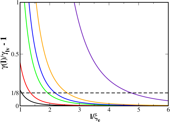
Figure 2: Plot of $\gamma(\ell)$ for a number of substrate/fluid pairs. From left to right water on quartz (black), octane on quartz (red), water on rutile (green), octane on $\alpha$-alumina (blue), octane on rutile (orange) and Liquid Helium on CaF₂ (indigo). The dashed horizontal line indicates a 1/8 increment over the asymptotic surface tension $\gamma_{lv}$.

V.2 Capillary wave broadening

Using Eq. (70) in either Eq. (11) or Eq. (12), we obtain for the thermally averaged density profile the following result:

$$\left\langle\rho(\mathbf{r};\mathcal{L})\right\rangle_{\Xi}=\rho_{\pi}(z;\ell)+\frac{1}{2}\frac{d^{2}\rho_{\pi}(z;\ell)}{dz^{2}}\Delta_{cw}^{2}$$ (79)

where $\Delta_{cw}^{2}$ dictates the amplitude of capillary wave broadening of the intrinsic density profile. Here, it is given as the sum of two different contributions:

$$\Delta_{cw}^{2}=\Delta_{0}^{2}+\Delta_{1}^{2}$$ (80)

The first one corresponds to the broadening due to mere translation of the profile, and corresponds to the result of classical capillary wave theory:

$$\Delta_{0}^{2}=\left\langle\delta\mathcal{L}^{2}\right\rangle_{\Xi}$$ (81)

The second one stems from distortions of the profile due to the finite gradient of interface fluctuations,MacDowell, Benet, and Katcho (2013); MacDowell et al. (2014) and unavoidably mixes intrinsic contributions (as dictated by $\xi_{e}$), and capillary wave distortions (as implied by the fluctuations of the film gradient):

$$\Delta_{1}^{2}=\xi_{e}^{2}\left\langle(\nabla_{\mathbf{x}}\mathcal{L})^{2}\right\rangle_{\Xi}$$ (82)

The intensity of specular reflectivity measurements consistent with the above results may be obtained by replacing Eq. (70) into Eq. (16):

$$I_{\rm spec}(Q_{z})=\rho_{\pi}(Q_{z})^{2}\left[1+Q_{z}^{2}\Delta_{cw}^{2}\right]$$ (83)

where $\rho_{\pi}(Q_{z})$ is the Fourier transform of $\rho_{\pi}(z)$, while $\Delta_{cw}^{2}$ is now given by Eq. (80), with:

$$\Delta_{0}^{2}=\sum_{\mathbf{q}}\left\langle\mathcal{L}^{2}(q)\right\rangle_{\Xi}$$ (84)

and

$$\Delta_{1}^{2}=\xi_{e}^{2}\sum_{\mathbf{q}}q^{2}\left\langle\mathcal{L}^{2}(q)\right\rangle_{\Xi}$$ (85)

Because of Parseval’s theorem, the results Eq. (81) and Eq. (84) for $\Delta_{0}^{2}$, as well as Eq. (82) and Eq. (85) for $\Delta_{1}^{2}$ are equivalent.

In order to obtain explicit results for $\Delta_{cw}^{2}$, we approximate the sum of Fourier components in Eq. (84) and Eq. (85) to an integral, i.e., $\sum_{\mathbf{q}}\to\frac{A}{4\pi^{2}}\int d\mathbf{q}$, and use Eq. (69) for the spectrum of surface fluctuations, whence:

$$\Delta_{cw}^{2}=\frac{k_{B}T}{2\pi}\int_{q_{min}}^{q_{max}}\frac{1+\xi_{e}^{2}q^{2}}{g^{\prime\prime}(\ell)+\gamma(\ell;q)q^{2}}d\mathbf{q}$$ (86)

where $q_{min}=2\pi/L$ is the lowest possible wave-vector consistent with the system’s lateral size, as dictated by $L$, while $q_{max}$ is an upper wave-vector cutoff. A closed expression for the general case of a fluid with short and long range forces (i.e., finite $\mu$) is not possible. Fortunately, recent studies suggest that the contribution of the singular term $q\ln q$ in $\gamma(\ell;q)$ is very small, so that most likely it is possible to describe $\Delta_{cw}^{2}$ assuming $\mu=0$.Chacón, Fernández, and Tarazona (2014) Also, notice the requirement of a finite interface width implies $\kappa(\ell)$ is a positive coefficient.Chacon and Tarazona (2005); Tarazona, Checa, and Chacon (2007); Höfling and Dietrich (2015) In that case, the integral may be solved analytically and approximated with good accuracy to the following result (Appendix E):

$$\begin{array}[]{lll}\Delta_{cw}^{2}&=&\displaystyle\frac{k_{B}T}{4\pi\gamma(\ell)}\left[\frac{\xi^{2}_{\parallel}-\xi^{2}_{e}}{\xi^{2}_{\parallel}-2\xi^{2}_{\kappa}}\right]\ln\left(\frac{1+\xi_{\parallel}^{2}q_{\rm max}^{2}}{1+\xi_{\parallel}^{2}q_{\rm min}^{2}}\right)\\ &&\\ &+&\displaystyle\frac{k_{B}T}{4\pi\kappa(\ell)}\left[\frac{\xi_{\parallel}^{2}\xi^{2}_{e}-(\xi^{2}_{e}+\xi_{\parallel}^{2})\xi^{2}_{\kappa}}{\xi_{\parallel}^{2}-2\xi^{2}_{\kappa}}\right]\ln\left(\frac{\xi_{\parallel}^{2}-(1-\xi_{\parallel}^{2}\,q_{\rm max}^{2})\xi^{2}_{\kappa}}{\xi_{\parallel}^{2}-(1-\xi_{\parallel}^{2}\,q_{\rm min}^{2})\xi^{2}_{\kappa}}\right)\end{array}$$ (87)

where $\xi_{\parallel}^{2}=\frac{\gamma(\ell)}{g^{\prime\prime}(\ell)}$ plays the role of a parallel correlation length for interface fluctuations and $\xi_{\kappa}^{2}=\frac{\kappa(\ell)}{\gamma(\ell)}$ may be interpreted as the length-scale below which bending the interface becomes too expensive. Notice that the contributions of gradient fluctuations in the interface roughening (Eq. (82) or Eq. (85)), may be readily recognized as those terms linear in $\xi_{e}^{2}$.

In the limit where both $\xi_{e}^{2}$ and $\xi_{\kappa}^{2}$ are allowed to vanish, Eq. (87) recovers the result of classical capillary wave theory, albeit with a film height dependent surface tension. Relaxing the constraint $\xi_{\kappa}^{2}=0$ while keeping $\xi_{e}^{2}=0$, Eq. (87) becomes an extended capillary wave theory that naturally provides an upper wave-vector cutoff $q_{\rm max}^{2}=\xi_{\kappa}^{-2}$. Taking into account the fluctuations of the film gradient requires to relax the constraint $\xi_{e}^{2}=0$, but in this case the bending rigidity coefficient $\kappa$ is not sufficient to provide for an ultraviolet cutoff.

In order to find plausible values for the unknown parameters $q_{max}$, and $\xi^{2}_{\kappa}$, in terms of $\xi_{e}$, it seems natural to consider the result for $\Delta_{cw}^{2}$ in the limit of vanishing external field ($\xi_{\parallel}^{2}\to\infty$):

$$\Delta_{cw}^{2}=\frac{k_{B}T}{2\pi\gamma_{lv}}\ln\left(\frac{q_{max}}{q_{min}}\right)-\frac{k_{B}T}{4\pi\gamma_{lv}}\left[1-\frac{\xi_{e}^{2}}{\xi_{\kappa}^{2}}\right]\ln(1+q_{max}^{2}\xi_{\kappa}^{2})$$ (88)

This result may be now compared with the expectations for the capillary wave broadening from the one-loop approximation, which holds precisely in that limit:Köpf and Münster (2008)

$$\Delta_{cw}^{2}=\frac{k_{B}T}{2\pi\gamma_{lv}}\ln\left(\frac{2\pi}{q_{min}\xi_{R}}\right)-\frac{k_{B}T}{4\pi\gamma_{lv}}\left[2\alpha-\frac{\pi^{2}}{2}\ln 3e^{-13/12}\right]$$ (89)

Since $\xi_{R}$ and $\xi_{e}$ describe the interface width of the intrinsic profile, we set $\xi_{R}=\xi_{e}$. It is then natural to equate Eq. (88) with Eq. (89) and to identify $\ln(q_{max}/q_{min})$ in the first expression with $\ln(2\pi/q_{min}\xi_{R})$ in the second. This then yields readily $q_{max}\approx 2\pi/\xi_{e}$ for the wave-vector cutoff and provides for the bending rigidity $\kappa\approx 4\gamma_{lv}\xi_{e}^{2}$ as the solution of a transcendental equation.

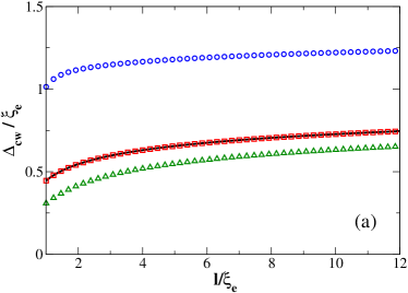
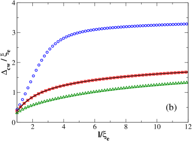
Figure 3: Plot of $\Delta_{cw}$ as given by Eq. (90) (symbols), compared to the classical theory (lines) for two substrate/fluid pairs (a), water adsorbed on quartz and (b), Liquid Helium adsorbed on CaF₂). Results are obtained for fixed $q_{max}=2\pi/\xi_{e}$, and a choice of bending rigidities, corresponding to $\xi_{\kappa}=\xi_{e}/2\pi$ (blue circles), $\xi_{\kappa}=\xi_{e}$ (red squares) and $\xi_{\kappa}=\sqrt{40/11}\xi_{e}$ (green triangles). The latter choice is suggested by the one-loop approximation. Notice that for intermediate film heights this choice requires evaluating $\Delta_{cw}^{2}$ with the exact result in complex algebra (see Appendix E). In all cases, $\xi_{e}=0.35$ nm.

Taking now the limit of large system sizes, $\xi_{\parallel}^{2}q_{min}^{2}\ll 1$, while allowing for a finite external field, which will usually be the relevant experimental situation, we find for the capillary wave broadening:

$$\Delta_{cw}^{2}=\frac{k_{B}T}{4\pi\gamma(\ell)}\left[\frac{\xi^{2}_{\parallel}-\xi^{2}_{e}}{\xi^{2}_{\parallel}}\right]\ln\left(\xi_{\parallel}^{2}q_{max}^{2}\right)+\frac{k_{B}T}{4\pi\gamma(\ell)}\left[\frac{\xi^{2}_{e}}{\xi_{\kappa}^{2}}-1\right]\ln\left(1+q_{max}^{2}\xi_{\kappa}^{2}\right)$$ (90)

We test this equation for strong to moderate external fields, by setting $q_{max}=2\pi/\xi_{e}$ as suggested above, while allowing for a choice of bending rigidities (Fig. 3). In the limit of very small external fields, $\xi^{2}_{\parallel}\to\infty$, our result becomes equal to that of classical capillary wave theory, except for an additive constant. However, in the presence of a tunable external field, classical theory predicts a broadening that is linear in $\ln\xi_{\parallel}^{2}$, while our theory of normal interface translations suggests the prefactor of the logarithmic term also depends on the external field.

In practice, the difference between Eq. (90) and the classical result (which is recovered simply by setting $\xi_{e}=0$) is mainly dictated by the second term in the right hand side of Eq. (90). If the ratio $\xi_{e}/\xi_{\kappa}$ differs from unity, it provides a nearly constant shift of the capillary wave broadening that may be either positive ($\xi_{\kappa}<\xi_{e}$) or negative ($\xi_{\kappa}>\xi_{e}$) and should be possible to distinguish experimentally (Fig. 3).

If, on the other hand $\xi_{e}/\xi_{\kappa}\to 1$, the shift vanishes altogether. In that case, the logarithmic contribution from Eq. (90) is hardly distinguishable from the classical result (Fig. 3).

In practice, $\xi_{\kappa}$ must be considered an empirical parameter, so that we cannot tell a priori the extent to which our result differs from the classical theory. By performing x-ray reflectivity experiments, it should be possible in principle to measure $\Delta_{cw}^{2}$ and confirm the expectations of Eq. (87) and Eq. (90) and to provide an estimate for $\xi_{\kappa}$. Interestingly, several x-ray diffraction experiments performed on fluid surfaces report the need to account for a constant shift on the results for $\Delta_{cw}$ which would be consistent with the expectations from Eq. (90) assuming $\xi_{\kappa}<\xi_{e}$.Ocko et al. (1994); Heilmann, Fukuto, and Pershan (2001); Plech et al. (2002) Unfortunately, it is not possible to distinguish whether this shift stems from the intrinsic width of the interface or from gradient fluctuations to the capillary wave broadening.

As a final remark, we note that, whereas the result of Eq. (88) for $\Delta_{cw}^{2}$ is consistent with the result of the one-loop approximation, Eq. (89), a stringent comparison of the individual components as implied in Eq. (80) does not seem to match so consistently.

Indeed, from Eq. (81)–Eq. (82) and Eq. (87), in the limit of vanishing external fields, we find:

$$\left\langle\delta\mathcal{L}^{2}\right\rangle_{\Xi}=\frac{k_{B}T}{2\pi\gamma_{lv}}\ln\left(\frac{q_{max}}{q_{min}(1+q_{max}^{2}\xi_{\kappa}^{2})^{1/2}}\right)$$ (91)

$$\left\langle(\nabla_{\mathbf{x}}\mathcal{L})^{2}\right\rangle_{\Xi}=\frac{k_{B}T}{4\pi\gamma_{lv}}\frac{\ln(1+q_{max}^{2}\xi_{\kappa}^{2})}{\xi_{\kappa}^{2}}$$ (92)

On the contrary, the comparison of Eq. (11) with the one-loop result of Eq. (20) suggests the fluctuations should be, rather:

$$\left\langle\delta\mathcal{L}^{2}\right\rangle_{\Xi}=\frac{k_{B}T}{2\pi\gamma_{lv}}\ln\left(\frac{2\pi\,e^{-\alpha}}{q_{min}\xi_{R}}\right)$$ (93)

$$\left\langle(\nabla_{\mathbf{x}}\mathcal{L})^{2}\right\rangle_{\Xi}=\frac{k_{B}T}{4\pi\gamma_{lv}}\frac{3}{2}\frac{\ln(3\,e^{-\frac{13}{12}})}{\xi_{R}^{2}}$$ (94)

Matching Eq. (91) with Eq. (93) and Eq. (92) with Eq. (94) provides a system of two equations with two unknowns, $q_{\max}$ and $\xi_{\kappa}$, but unfortunately, the only solution yields the result $q_{max}^{-2}=244\xi_{e}^{2}$ and $\kappa=-243\gamma_{lv}\xi_{e}^{2}$. The origin of the unexpected small cutoff and negative $\kappa$ lies in the result for $\left\langle(\nabla\mathcal{L})^{2}\right\rangle_{\Xi}$ in Eq. (94), which is close to zero (since $\ln 3-13/12\approx 0$) and can only match Eq. (92) if we accept a negative $\kappa$.

The difference of this unsatisfactory comparison with that performed previously, which provided results for $q_{max}$ and $\kappa$ closer to expectations is whether one interprets the term $-\frac{k_{B}T}{2\pi\gamma}\alpha$ in Eq. (89) as belonging to either $\left\langle(\delta\mathcal{L})^{2}\right\rangle_{\Xi}$ or $\left\langle(\nabla\mathcal{L})^{2}\right\rangle_{\Xi}$. In view of this discussion, the latter interpretation seems more justified.

VI Comparison with exact results

Before closing, we test our results with an exact solution of the Landau-Ginzburg-Wilson Hamiltonian under an external field. A solution of this system for arbitrary external fields $V(z)$, is generally not possible. However, in an exceptional and somewhat forgotten paper, Zittartz noticed many years ago that this problem may be remedied for an external field of $\tanh(z)$ form.Zittartz (1967)

Particularly, Zittartz considered the free energy functional Eq. (31) in the lattice gas analogue, with the usual biquadratic bulk free energy $f(\rho)=\alpha\rho^{4}-\epsilon\rho^{2}$ and an external field:

$$V(z)=2u\left(\frac{\epsilon+u}{2\alpha}\right)^{1/2}\tanh\left(\frac{1}{2}\frac{z-\ell}{\xi_{u}}\right)$$ (95)

where

$$\xi_{u}=\frac{1}{2}\left(\frac{\epsilon+u}{C}\right)^{-1/2}$$ (96)

This external field is unusual, because it has its origin at the interface position. Accordingly, the free energy depends only on the field strength $u$, and not on the interface position.

The exact mean field (intrinsic) density profile is:Zittartz (1967)

$$\rho_{\pi}(z)=\left(\frac{\epsilon+u}{2\alpha}\right)^{1/2}\tanh\left(\frac{1}{2}\frac{z-\ell}{\xi_{u}}\right)$$ (97)

Notice that the role of $V(z)$ is to pin exactly the interface at $z=\ell$ and set the interface width $\xi_{u}$.

Armed with this solution, we can now assess several of the results of section IV.1, IV.5 and V.1.

First consider the surface tension as predicted by the Fisher-Jin theory for a system with short range forces in an external field $V_{0}(z)$ equal to $V(z)$ above. Using Eq. (43), with Eq. (97) for the density, we obtain in closed form:

$$\gamma_{u}=\frac{2}{3}\frac{C^{1/2}}{\alpha}(\epsilon+u)^{3/2}$$ (98)

where we have added the subindex $u$ next to $\gamma_{u}$ in order to stress the explicit dependece on the external field that we have assumed.

Clearly, as $u\to 0$, $\gamma_{u}$ splits into $\gamma_{0}=\frac{2}{3}\frac{C^{1/2}}{\alpha}\epsilon^{3/2}$, for the surface tension in zero field, and $\Delta\gamma=\frac{(\epsilon C)^{1/2}}{\alpha}u$ for linear corrections in the field strength.

Now consider the perturbative result, Eq. (49), for the correction of $\gamma_{0}$ due to the external field $V(z)$, which, using again Eq. (97) for the density yields:

$$\Delta\gamma=\frac{C^{1/2}(\epsilon+u)^{1/2}}{\alpha}u$$ (99)

Clearly, in the limit $u\to 0$, this result provides exactly the same leading order correction to $\gamma_{u}$ that was obtained using $Eq.~{}(\ref{eq:gammasgtv1})$ in the paragraph above. This attests to the consistency of our approach. Particularly, it shows that the approximation used in Eq. (49) remains very robust, even though Eq. (37) does not yield the exact limit of density decay at infinity.

Now, consider the calculation of $g^{\prime\prime}$, which can be performed by plugin the density profile of Eq. (97) into Eq. (72). Again, the result may be obtained in closed form as:

$$g^{\prime\prime}_{ext}=\frac{4}{3}\frac{(\epsilon+u)^{3/2}}{\alpha C^{1/2}}u$$ (100)

using the result for the bulk correlation length in zero field, $\xi_{0}^{2}=\frac{1}{4}C/\epsilon$, together with $\Delta\gamma=g^{\prime\prime}\xi_{0}^{2}$ (c.f. Eq. (71)) we find, to linear order in the field strength:

$$\Delta\gamma=\frac{1}{3}\frac{(C\epsilon)^{1/2}}{\alpha}u$$ (101)

Whence, the approximate solution Eq. (71), provides also the correct result, with an empirical measure of the interface width $\xi_{e}=\sqrt{3}\xi_{0}$. This is a very handy result, because most often neither the density profile nor the external field are known. Therefore, the explcit results Eq. (43) or Eq. (49) are not practical. On the contrary, the first derivative $g^{\prime}$ is the negative of the disjoining pressure and can be measured experimentally.

So far we have tested that the alternative results Eq. (43), Eq. (49) and Eq. (73) for the film height dependent surface tension are consistent. But it remains to show that these corrections to the surface tension have their signature stamped in the spectrum of surface fluctuations, as suggested in Eq. (69).

To show this, consider the density-density correlation function predicted by capillary wave theory, Eq. (17):

$$G_{cw}(z_{1},z_{2}{};q)=\frac{d\rho_{\pi}(z_{1})}{d\ell}\frac{d\rho_{\pi}(z_{2})}{d\ell}\left\langle\mathcal{L}^{2}(q)\right\rangle$$ (102)

with $\left\langle\mathcal{L}^{2}(q)\right\rangle$ given by Eq. (69).

This result may be compared with the correlation function of the Landau-Ginzburg-Wilson Hamiltonian as discussed by Zittartz and Jasnow.Zittartz (1967); Jasnow (1984) Exact solutions exist in closed form.Zittartz (1967) However, for this system it is more convenient to exploit the fact that $G(\mathbf{r}_{1},\mathbf{r}_{2})$ is a Green’s function. Accordingly, it may be expressed as an eigenvalue expansion as follows:

$$G(z_{1},z_{2}{};q)=\sum_{n}\frac{\phi^{*}_{n}(z_{1})\phi_{n}(z_{2})}{\lambda_{n}}$$ (103)

where $\phi_{n}(z)$ and $\lambda_{n}$ are the solutions of the eigenvalue equation:

$$\left[-C\frac{d^{2}}{dz^{2}}+Cq^{2}-2\epsilon+12\alpha\rho_{\pi}^{2}(z)\right]\phi(z)=\lambda\phi(z)$$ (104)

In the quantum mechanical analogy, with $\rho_{\pi}(z)$ of hyperbolic tangent form, this is the Schrödinger equation for a shifted Pöschl-Teller potential, whose exact solutions are well known.Lekner (2007)

The first two eigenvalues of the Pöschl-Teller well correspond to states bound to the potential, which are naturally related to purely interfacial contributions to the correlation function. The remaining eigenvalues lay in the continuum and may be considered as corresponding to bulk correlations perturbed by the interface.

The bound state of lowest energy is a soft mode which merely describes the displacement of the interface, without change of the density profile.Zittartz (1967); Jasnow (1984) Its eigenfunction is $\phi_{1}(z)=d\rho_{\pi}/dz$, and the corresponding eigenvalue is:

$$\lambda_{1}=2u+Cq^{2}$$ (105)

Clearly, in the limit of $u\to 0$, $\lambda_{1}\propto q^{2}$, and we can therefore identify this mode as the translation mode of the capillary wave Hamiltonian. As the field is switched on, the first eigenvalue merely describes how the translational mode is modified by the external field.

From Eq. (98) and Eq. (100), one readily finds that the ratio $\frac{1}{2}C/u$ is precisely the ratio of $\gamma_{u}$ to $g^{\prime\prime}$ in the Zittartz model. Accordingly, it follows that, under the external field, Eq. (95), the translational mode of the correlation function is:

$$G_{\rm tras}(z_{1},z_{2}{};q)\propto\frac{d\rho_{\pi}(z_{1})}{d\ell}\frac{d\rho_{\pi}(z_{2})}{d\ell}\frac{k_{B}T}{g^{\prime\prime}+\gamma_{u}q^{2}}$$ (106)

where $\gamma_{u}$ is given exactly to linear order in the field strength by either Eq. (43) or Eq. (49).

Comparison of this result with Eq. (102) in the limit of small wave-vectors $q\ll\kappa$, indicates that our result for the spectrum of interface fluctuations, Eq. (69), is also exact to linear order in $u$.

This reveals clearly the strengths and limitations of the capillary wave approach. On the one hand, we have showed that considering explicitely perpendicular rather than merely vertical translations of the interface is sufficient to describe exactly to linear order in the field strength the long wavelength surface fluctuations of the translational mode. On the other hand, capillary wave theory, up to this level of detail, cannot do anything else. i.e., the remaining surface mode, with explicit $q$ dependence is completely beyond reach, and cannot be described at all without considering explicitely perturbations of the intrinsic density profile. Likewise, modes in the continuum, which can be identified with bulk correlations perturbed by the interface, are also beyond the level of description that can be achieved with capillary wave theory. Presumably, the non-local theory of interfaces shares similar limitations, since there the corrections to the density profile are given merely by the bulk correlation function.Bernardino et al. (2009) Some of these limitations have been discussed by studying the correlation function of the double parabola model, which, unlike more elaborate biquadratic free energies, has only one bound surface state.Parry, Rascón, and Evans (2015) A promising approach to single out the surface translation mode from the full correlation function has been suggested recently.Hernández-Muñoz, Chacón, and Tarazona (2016)

VII Conclusions

In this paper we have considered the phenomenological extension of classical capillary wave theory to the case were the density is dictated by the normal distance to the local interface position (Eq. (2)). This idea seems justified on intuitive grounds and symmetry considerations, at least for long wave-length fluctuations in the absence of an external field. Recently, it has been shown that the hypothesis remains accurate even for liquid films close to the three phase contact line.Nold et al. (2016) Not surprisingly, the approach has been explored previously, starting with an apparently overlooked contribution by Davis many years ago.Davis (1977); Diehl, Kroll, and Wagner (1980); Kawasaki and Ohta (1982); Stecki (1998, 2001); Mecke and Dietrich (1999) However, it would seem that some important consequences had not been recognized. Other recent studies have rather attempted to assess the role of interface curvature.Mecke and Dietrich (1999); Blokhuis (2009); Parry and Rascón (2011) Such effects can be incorporated as an effective wave-vector dependent surface tension, and appear as corrections of order $q^{4}$ in the capillary wave spectrum. Unfortunately, it would seem that both on theoretical and experimental grounds the study of such corrections from the spectrum of surface fluctuations poses serious difficulties.Tarazona, Checa, and Chacon (2007); Parry, Rascón, and Evans (2015) On the other hand, we have shown that in the presence of an external-field the assumption of an interface profile along lines normal to the interface results in the coupling of surface and bulk fluctuations. This produces corrections of order $q^{2}$ which feed into the surface tension and are linear in $g^{\prime\prime}_{ext}(\ell)$.MacDowell, Benet, and Katcho (2013); MacDowell et al. (2014); Benet et al. (2014) Comparing our results to a more formal approach based on linear response theory indicates that the simple phenomenological extension considered here might be sufficient to identify the most relevant corrections to the classical theory for flat substrates away from the strong fluctuating regime.Bernardino et al. (2009)

The first, and most immediate implication of our approach is that already to first order in deviations from planarity, the theory picks up an additional capillary wave broadening mechanism, with contributions that are given by the fluctuations of the film profile gradient (Eq. (11)). Such additional broadening may be captured in terms of a ‘convolution’ approximation, by assuming that the normal distance of a point to the interface is Gaussian distributed (Eq. (12)). The effect on the average density profile could be measured in principle by the specular contribution to x-ray surface scattering (Eq. (16)).

In the absence of an external field, we show that this phenomenological theory is consistent with renormalization group theory in the one loop approximation.Jasnow and Rudnick (1978); Köpf and Münster (2008) The success of this comparison indicates that it is meaningful to decouple bulk and capillary wave fluctuations even close to the critical point, or equivalently, that one can assume the Fisk-Widom scaling form of a density profile prior to renormalization of capillary wave-fluctuations. This holds provided the density is given along normals to the film profile (Eq. (21)). Applying this condition to a Cahn-Hillard square gradient approximation, one recovers the capillary wave Hamiltonian exactly in the limit of small curvature (Eq. (29)).Davis (1977); Huse, van Saarloos, and Weeks (1985)

We have further extended the theory of normal translations to the case of adsorbed liquid films (Eq. (34)). For systems of short range forces only, this recovers the Fisher-Jin theory of short range wetting (Eq. (40),Eq. (43)),Jin and Fisher (1993); Fisher, Jin, and Parry (1994) and introduces a film height dependence of the surface tension which has been identified recently in computer simulation experiments.Fernández, Chacón, and Tarazona (2012); Fernández et al. (2015) In the presence of a long range forces, the external field couples to the film gradient fluctuations, and results in an explicit dependence of the surface tension on the field that is consistent with expectations from the Non-Local theory of interfaces (Eq. (49)).Bernardino et al. (2009) The signature of this coupling appears explicitely in the spectrum of surface fluctuations, Eq. (69). Comparison with results for an exactly solvable model of the LGW Hamiltonian in an external field indicate that Eq. (69), together with either Eq. (43) and Eq. (49) reproduces exactly to linear order in field strength the translational mode of the density correlation function (c.f: section VI). Including long-range dispersive forces, the theory yields the well known logarithmic singularity of the wave-vector dependent surface tension (Eq. (62),Eq. (67)).Napiórkowski and Dietrich (1993); Mecke and Dietrich (1999); Blokhuis (2009)

We have studied a simple model of adsorbed films which assumes the liquid-vapor density profile is independent of the proximity to the substrate and takes the form of an error function. Under this simplifying assumption, our approach allows to write the film height dependent surface tension explicitly in terms of the disjoining pressure (Eq. (73)). For wetting films, this results in a strong enhancement of the surface tension that has been verified in computer simulation experiments.MacDowell, Benet, and Katcho (2013); Benet et al. (2014) Our qualitative calculations indicate that the range where the film height dependent surface tension may be measured lays in the sub-nanometer range (Table 1). For such thin films, the corrections to classical theory become significant and could be measured in principle by means of x-ray scattering experiments (Eq. (90)), where the specular reflectivity allows to measure the interface width, $\Delta_{cw}$ while the diffuse scattering probes the exponent $\eta\propto k_{B}T/\gamma$.Doerr et al. (1998); Pershan and Schlossman (2012) Experimental observation of a larger $\Delta_{cw}$ and a smaller $\eta$ than expected from the classical theory would provide strong indications in support of our conclusions. Unfortunately, this task requires to disentangle the purely translational mode of surface fluctuations from additional surface and bulk correlations, which seems difficult at present without a very accurate model for the full inhomogeneous pair correlation function.Hernández-Muñoz, Chacón, and Tarazona (2016) Alternatively, these corrections could become important when attempting to extend the capillarity approximation to adsorbed films at the nanoscale, as revealed by recent computer simulations and atomic force microscopy experiments which indicate the need to account for an enhanced surface tension.Asay and Kim (2006); Laube et al. (2015)

Appendix A Derivation of Eq. (16) and Eq. (17)

In order to obtain Eq. (16) and Eq. (17), we notice that all odd terms in $\mathcal{L}(\mathbf{x})$ vanish after thermal averaging of the density correlation function, Eq. (14). This means that $\langle\delta s\rangle$ only retains the term in $(\nabla\delta\mathcal{L})^{2}$. For this reason, we can write:

$$\begin{array}[]{lll}\int d\mathbf{x}_{1}d\mathbf{x}_{2}\langle\delta s(\mathbf{x})\rangle e^{i{\bf Q}_{\mathbf{x}}\cdot(\mathbf{x}_{1}-\mathbf{x}_{2})}&=&\frac{1}{2}\int d\mathbf{x}\,d\Delta\mathbf{x}\,\langle(z-\ell)\sum_{\bf q}{\bf q}\,\mathcal{L}({\bf q})e^{i{\bf q}\cdot\mathbf{x}}\cdot\sum_{\bf q^{\prime}}{\bf q^{\prime}}\mathcal{L}({\bf q}^{\prime})e^{i{\bf q}^{\prime}\cdot\mathbf{x}}\rangle\,e^{i{\bf Q}_{\mathbf{x}}\cdot\Delta\mathbf{x}}\\ &&\\ &=&\frac{1}{2}(z-\ell)\sum_{\bf q}q^{2}\langle\mathcal{L}^{2}({\bf q})\rangle\;\delta({\bf Q}_{\mathbf{x}})\end{array}$$ (107)

where we have expressed $\nabla\mathcal{L}(\mathbf{x})$ as an expansion in Fourier modes, and performed the change of variables $\Delta\mathbf{x}=\mathbf{x}_{1}-\mathbf{x}_{2}$. For the average $\langle\delta s^{2}\rangle$, we proceed likewise and write:

$$\begin{array}[]{lll}\int d\mathbf{x}_{1}d\mathbf{x}_{2}\langle\delta s^{2}(\mathbf{x})\rangle e^{i{\bf Q}_{\mathbf{x}}\cdot(\mathbf{x}_{1}-\mathbf{x}_{2})}&=&\frac{1}{2}\int d\mathbf{x}\,d\Delta\mathbf{x}\,\langle(z-\ell)\sum_{\bf q}\mathcal{L}({\bf q})e^{i{\bf q}\cdot\mathbf{x}}\sum_{\bf q^{\prime}}\mathcal{L}({\bf q}^{\prime})e^{i{\bf q}^{\prime}\cdot\mathbf{x}}\rangle e^{i{\bf Q}_{\mathbf{x}}\cdot\Delta\mathbf{x}}\\ &&\\ &=&\sum_{\bf q}\langle\mathcal{L}^{2}({\bf q})\rangle\delta({\bf Q}_{\mathbf{x}})\end{array}$$ (108)

where all terms beyond quadratic order in the Fourier amplitudes $\mathcal{L}({\bf q})$ have been ignored. Finally, for the crossed correlations we write:

$$\begin{array}[]{lll}\int d\mathbf{x}_{1}d\mathbf{x}_{2}\langle\delta s(\mathbf{x}_{1})\delta s(\mathbf{x}_{2})\rangle e^{i{\bf Q}_{\mathbf{x}}\cdot(\mathbf{x}_{1}-\mathbf{x}_{2})}&=&\int d\mathbf{x}_{1}\,d\mathbf{x}_{2}\,\langle\mathcal{L}(\mathbf{x}_{1})\mathcal{L}(\mathbf{x}_{2})\rangle e^{i{\bf Q}_{\mathbf{x}}\cdot(\mathbf{x}_{1}-\mathbf{x}_{2})}\\ &&\\ &=&\langle\mathcal{L}^{2}({\bf Q}_{\mathbf{x}})\rangle\end{array}$$ (109)

Using these transforms in Eq. (13), we obtain Eq. (16) and Eq. (17).

Appendix B Derivation of Eq. (39)

In order to arrive at Eq. (39), we need to consider the derivatives of $\rho_{\pi}(z;\ell)$ for an adsorbed film, which for symmetry reasons depends explicitly on two variables, the distance from the wall, $z$, and the film height, $\ell$. This differs from the case of a free interface, where $\rho_{\pi}$ is a function of the single variable, $z-\ell$. Also it is required to take into account that, by virtue of Eq. (34), $\rho_{\pi}(z;\ell)$ is evaluated for a film height, $\ell=\mathcal{L}+\delta s$ which depends explicitly on $\mathbf{x}$ and $z$. Whence:

$$\nabla\rho_{\pi}(z;\ell=\mathcal{L}+\delta s)=\left(\frac{\partial\rho_{\pi}}{\partial z}+\frac{\partial\rho_{\pi}}{\partial\ell}\frac{d\ell}{dz}\right){\bf k}+\frac{\partial\rho_{\pi}}{\partial\ell}\nabla_{\mathbf{x}}\ell$$ (110)

where ${\bf k}$ is a unit vector in the $z$ direction. To quadratic order in $\mathcal{L}$, the squared gradient is then given as:

$$\left(\nabla\rho_{\pi}(z;\ell=\mathcal{L}+\delta s)\right)^{2}=\left(\frac{\partial\rho_{\pi}}{\partial z}\right)^{2}+\frac{\partial\rho_{\pi}}{\partial z}\frac{\partial\rho_{\pi}}{\partial\ell}\left(\nabla_{\mathbf{x}}\mathcal{L}\right)^{2}+\left(\frac{\partial\rho_{\pi}}{\partial\ell}\right)^{2}\left(\nabla_{\mathbf{x}}\mathcal{L}\right)^{2}$$ (111)

where we have employed $d\ell/dz=\frac{1}{2}(\nabla_{\mathbf{x}}\mathcal{L})^{2}$. Notice that all terms in the right hand side of Eq. (111) are evaluated at $\ell=\mathcal{L}+\delta s$. In order to arrive at Eq. (39), which has the density profiles evaluated at the film height $\ell=\mathcal{L}$, we expand in powers of $\delta s$. Since we are only interested in contributions of order $(\nabla_{\mathbf{x}}\mathcal{L})^{2}$, at most, it suffices to expand only the first term to linear order in $\delta s$, and retain the second and third terms to obtain Eq. (39).

Appendix C Stationarity at the boundary and alternative derivation of Eq. (43)

In the minimization of Eq. (31), the density at the wall is not prescribed a-priori, but must rather be given as a solution of the variational problem. For this reason, Eq. (32) is necessary but not sufficient condition. To see this, we follow Ref.Parry et al., 2006, and use $\nabla\rho_{\pi}\cdot\nabla\delta\rho=\nabla\cdot(\nabla\rho_{\pi}\delta\rho)-\nabla^{2}\rho_{\pi}\delta\rho$ in Eq. (33), together with the divergence theorem. The stationary condition then becomes:

$$\int d\mathbf{r}\,\delta\rho\left\{\frac{\partial f}{\partial\rho}-C\nabla^{2}\rho_{\pi}+V_{0}\right\}+\int dS\,\delta\rho\,C\nabla\rho_{\pi}\cdot{\bf n}=0$$ (112)

where n is a unit vector perpendicular to the wall, and $dS$ denotes integration over the surface of the wall. In variational problems where $\rho_{\pi}$ at the surface is prescribed the surface term vanishes and Eq. (32) is sufficient to solve the variational problem. Here, we can neither assume a priori $\delta\rho=0$, nor $\nabla\rho_{\pi}=0$ at the wall, and the surface term must be retained.

In order to obtain Eq. (43), we eliminate the integral over the first square brackets of Eq. (42) using Eq. (112) with the choice $\delta\rho=(z-\mathcal{L})\frac{\delta\rho_{\pi}}{\delta\ell}$. Performing an integration by parts two of the three terms in the resulting integral mutually cancel each other, and we are left with Eq. (43).

Appendix D Surface properties of a substrate-fluid pair interacting via the Sutherland potential

The Sutherland potential is:

$$u=\left\{\begin{array}[]{ll}\infty&\quad\quad r<\sigma\\ &\\ -C/r^{6}&\quad\quad r>\sigma\end{array}\right.$$ (113)

In what follows, we write the constant $C$ as $C=\sigma^{6}\epsilon$.

Using the results from Ref.Dietrich and Schick (1986) and the integrals for $-C/r^{6}$ from Ref.de Gregorio et al. (2012), we obtain, after very tedious but straightforward manipulations:

$$\gamma_{lv}=\frac{1}{4}\pi\epsilon\sigma^{4}(\rho_{l}-\rho_{v})^{2}$$ (114)

$$\gamma_{w\beta}=\frac{1}{4}\pi\epsilon_{w}\sigma_{w}^{4}(\rho_{w}-\rho_{\beta})^{2}+\frac{5\pi}{12}\epsilon_{w}\sigma_{w}^{4}\rho_{w}\rho_{\beta}$$ (115)

for $\beta={l,v}$.

$$A_{w}=\pi^{2}(\rho_{v}-\rho_{l})(\epsilon_{w}\sigma_{w}^{6}\rho_{w}-\epsilon\sigma^{6}\rho_{l})$$ (116)

Defining the spreading coefficient as $S=(\gamma_{wv}-\gamma_{wl})/\gamma_{lv}$, we obtain:

$$S=\frac{\frac{7}{6}\epsilon_{w}\sigma_{w}^{4}\rho_{w}-\epsilon\sigma^{4}(\rho_{l}+\rho_{v})}{\epsilon\sigma^{4}(\rho_{l}-\rho_{v})}$$ (117)

For $\rho_{l}\gg\rho_{v}$ and $\sigma_{w}\approx\sigma$, we find the spreading coefficient becomes:

$$S\approx-\frac{A_{w}}{A_{l}}$$ (118)

where

$$A_{l}=\pi^{2}\epsilon\sigma^{4}\rho_{l}^{2}$$ (119)

The results of this appendix improve our previous estimates of the surface properties of the Sutherland model.de Gregorio et al. (2012) The key point is the precise evaluation of the dispersion integrals within perpendicular distances $|z|<\sigma$. For $\gamma_{lv}$, for example, our results may now be cast in terms of $A_{l}$ as $\gamma_{lv}=A_{l}/4\pi\sigma^{2}$, which is very nearly equal to the empirical result $\gamma_{lv}=\frac{25}{24}\frac{A_{l}}{4\pi\sigma^{2}}$ advocated by Israelachvili.Israelachvili (1991)

Appendix E Derivation of Eq. (87)

Here we solve the indefinite integral that is required to obtain $\Delta_{cw}^{2}$ in Eq. (87).

$$I=\int\frac{q+\xi_{e}^{2}q^{3}}{g^{\prime\prime}+\gamma q^{2}+\kappa q^{4}}\,dq$$ (120)

In principle this integral may be obtained readily in terms of $\arctan$ functions, but this expression involves complex numbers and does not allow for an obvious comparison with the results of classical capillary wave theory ($\xi_{e}=0$, $\kappa=0$), which is given in terms of the logarithmic function. In order to reveal the similarities between both results, we factor the denominator as:

$$g^{\prime\prime}+\gamma q^{2}+\kappa q^{4}=(a+\gamma q^{2})(r+\frac{\kappa}{\gamma}\,q^{2})$$ (121)

under the requirement that it becomes equal to the first factor in the right hand side in the limit $\kappa\to 0$. Solving for $a$ and $r$, we find:

$$\left\{\begin{array}[]{lll}a&=&\frac{g^{\prime\prime}}{r}\\ r&=&\frac{1}{2}\left(1+\sqrt{1-4g^{\prime\prime}\kappa/\gamma^{2}}\right)\end{array}\right.$$ (122)

Having factored the denominator, the integral may be solved by the technique of partial fractions,Kouba yielding:

$$I=\frac{1}{2}\frac{r\gamma-\xi_{e}^{2}g^{\prime\prime}}{r^{2}\gamma^{2}-g^{\prime\prime}\kappa}\ln(g^{\prime\prime}+\gamma rq^{2})+\frac{1}{2}\frac{\gamma r}{\kappa}\frac{\xi_{e}^{2}\gamma r-\kappa}{r^{2}\gamma^{2}-g^{\prime\prime}\kappa}\ln(\gamma r+\kappa q^{2})$$ (123)

Eq. (87) is recovered from this result in the limit of $4g^{\prime\prime}\kappa/\gamma^{2}\ll 1$. In practice, we checked that Eq. (87) provides a very robust approximation to the exact result in physically relevant situations considered previously.MacDowell, Benet, and Katcho (2013)

References

- Höfling and Dietrich (2015) F. Höfling and S. Dietrich, Europhys. Lett 109, 46002 (2015).
- Parry, Rascón, and Evans (2015) A. O. Parry, C. Rascón, and R. Evans, ArXiv 1510.00314v1, 1 (2015).
- Chacón and Tarazona (2016) E. Chacón and P. Tarazona, J. Phys.: Condens. Matter 28, 244014 (2016).
- Evans (1979) R. Evans, Adv. Phys. 28, 143 (1979).
- Evans (1992) R. Evans, in Fundamentals of Inhomogenous Fluids, edited by D. Henderson (Marcel Dekker, New York, 1992) Chap. 3, pp. 85–175.
- Fisk and Widom (1969) S. Fisk and B. Widom, J. Chem. Phys. 50, 3219 (1969).
- Rowlinson and Widom (1982) J. Rowlinson and B. Widom, Molecular Theory of Capillarity (Clarendon, Oxford, 1982).
- Zittartz (1967) J. Zittartz, Phys. Rev. 154, 529 (1967).
- Jasnow and Rudnick (1978) D. Jasnow and J. Rudnick, Phys. Rev. Lett. 41, 698 (1978).
- Evans and Wilding (2015) R. Evans and N. B. Wilding, Phys. Rev. Lett. 115, 016103 (2015).
- Abraham (1981) D. B. Abraham, Phys. Rev. Lett. 47, 545 (1981).
- Jasnow (1984) D. Jasnow, Rep. Prog. Phys. 47, 1059 (1984).
- Köpf and Münster (2008) M. H. Köpf and G. Münster, J. Stat. Phys. 132, 417 (2008).
- Delfino and Viti (2012) G. Delfino and J. Viti, J. Stat. Mech. 2012, P10009 (2012).
- Buff, Lovett, and Stillinger (1965) F. P. Buff, R. A. Lovett, and F. H. Stillinger, Phys. Rev. Lett. 15, 621 (1965).
- Weeks (1977) J. D. Weeks, J. Chem. Phys. 67, 3106 (1977).
- Bedeaux and Weeks (1985) D. Bedeaux and J. D. Weeks, J. Chem. Phys. 82, 972 (1985).
- Huse, van Saarloos, and Weeks (1985) D. A. Huse, W. van Saarloos, and J. D. Weeks, Phys. Rev. B 32, 233 (1985).
- Fisher, Fisher, and Weeks (1982) M. P. A. Fisher, D. S. Fisher, and J. D. Weeks, Phys. Rev. Lett. 48, 368 (1982).
- Braslau et al. (1988) A. Braslau, P. S. Pershan, G. Swislow, B. M. Ocko, and J. Als-Nielsen, Phys. Rev. A 38, 2457 (1988).
- Ocko et al. (1994) B. M. Ocko, X. Z. Wu, E. B. Sirota, S. K. Sinha, and M. Deutsch, Phys. Rev. Lett. 72, 242 (1994).
- Doerr et al. (1999) A. K. Doerr, M. Tolan, W. Prange, J.-P. Schlomka, T. Seydel, W. Press, D. Smilgies, and B. Struth, Phys. Rev. Lett. 83, 3470 (1999).
- Benjamin (1992) I. Benjamin, J. Chem. Phys. 97, 1432 (1992).
- Müller and Schick (1996) M. Müller and M. Schick, J. Chem. Phys. 105, 8885 (1996).
- Lacasse, Grest, and Levine (1998) M.-D. Lacasse, G. S. Grest, and A. J. Levine, Phys. Rev. Lett. 80, 309 (1998).
- Vink, Horbach, and Binder (2005) R. L. C. Vink, J. Horbach, and K. Binder, J. Chem. Phys. 122, 134905 (2005).
- Davis (1977) H. T. Davis, J. Chem. Phys. 67, 3636 (1977).
- Napiórkowski and Dietrich (1993) M. Napiórkowski and S. Dietrich, Phys. Rev. E 47, 1836 (1993).
- Robledo and Varea (1997) A. Robledo and C. Varea, J. Stat. Phys. 89, 273 (1997).
- Mecke and Dietrich (1999) K. R. Mecke and S. Dietrich, Phys. Rev. E 59, 6766 (1999).
- Stecki (2001) J. Stecki, J. Chem. Phys. 114, 7574 (2001).
- Blokhuis (2009) E. M. Blokhuis, J. Chem. Phys. 130, 014706 (2009).
- Paulus, Gutt, and Tolan (2008) M. Paulus, C. Gutt, and M. Tolan, Phys. Rev. B 78, 235419 (2008).
- Pershan and Schlossman (2012) P. S. Pershan and M. Schlossman, Liquid Surfaces and Interfaces: Synchrotron X-ray Methods (Cambridge University Press, Cambridge, 2012).
- Chacon and Tarazona (2003) E. Chacon and P. Tarazona, Phys. Rev. Lett. 91, 166103 (2003).
- Chacon and Tarazona (2005) E. Chacon and P. Tarazona, J. Phys.: Condens. Matter 17, S3493 (2005).
- Tarazona, Checa, and Chacon (2007) P. Tarazona, R. Checa, and E. Chacon, Phys. Rev. Lett. 99, 196101 (2007).
- Parry and Rascón (2009) A. O. Parry and C. Rascón, J. Low Temp. Phys. 157, 149 (2009).
- Bryk and Binder (2013) P. Bryk and K. Binder, Phys. Rev. E 88, 030401 (2013).
- Jin and Fisher (1993) A. J. Jin and M. E. Fisher, Phys. Rev. B 47, 7365 (1993).
- Parry et al. (2006) A. O. Parry, C. Rascón, N. R. Bernardino, and J. M. Romero-Enrique, J. Phys.: Condens. Matter 18, 6433 (2006).
- Fernández, Chacón, and Tarazona (2012) E. M. Fernández, E. Chacón, and P. Tarazona, Phys. Rev. B 86, 085401 (2012).
- Fernández et al. (2015) E. M. Fernández, E. Chacón, L. G. MacDowell, and P. Tarazona, Phys. Rev. E 91, 062404 (2015).
- MacDowell, Benet, and Katcho (2013) L. G. MacDowell, J. Benet, and N. A. Katcho, Phys. Rev. Lett. 111, 047802 (2013).
- MacDowell et al. (2014) L. G. MacDowell, J. Benet, N. A. Katcho, and J. M. Palanco, Adv. Colloid Interface Sci. 206, 150 (2014).
- Benet et al. (2014) J. Benet, J. G. Palanco, E. Sanz, and L. G. MacDowell, J. Phys. Chem. C 118, 22079 (2014).
- Bernardino et al. (2009) N. R. Bernardino, A. O. Parry, C. Rascón, and J. M. Romero-Enrique, J. Phys.: Condens. Matter 21, 465105 (2009).
- Werner et al. (1999) A. Werner, M. Muller, F. Schmid, and K. Binder, J. Chem. Phys. 110, 1221 (1999).
- Diehl, Kroll, and Wagner (1980) H. W. Diehl, D. M. Kroll, and H. Wagner, Z. Phys. B 36, 329 (1980).
- Kawasaki and Ohta (1982) K. Kawasaki and T. Ohta, Prog. Theor. Phys. 67, 147 (1982).
- Nold et al. (2014) A. Nold, D. N. Sibley, B. D. Goddard, and S. Kalliadasis, Phys. Fluids 26, 072001 (2014).
- Hughes, Thiele, and Archer (2015) A. P. Hughes, U. Thiele, and A. J. Archer, J. Chem. Phys. 142, 074702 (2015).
- Nold et al. (2015) A. Nold, D. N. Sibley, B. D. Goddard, and S. Kalliadasis, ArXiv preprint , arXiv:1503.03232 (2015), accepted for publication in Math. Model. Nat. Phenom.
- Nold et al. (2016) A. Nold, L. G. MacDowell, D. N. Sibley, B. D. Goddard, and S. Kalliadasis, (2016), submitted to Phys. Fluids.
- Willard and Chandler (2010) A. P. Willard and D. Chandler, The Journal of Physical Chemistry B 114, 1954 (2010), pMID: 20055377, http://dx.doi.org/10.1021/jp909219k .
- Zia (1985) R. Zia, Nuclear Phys. B 251, 676 (1985).
- Fisher, Jin, and Parry (1994) M. E. Fisher, A. J. Jin, and A. O. Parry, Ber. Bunsenges. Phys. Chem. 98, 357 (1994).
- Safran (1994) S. A. Safran, Statistical Thermodynamics of Surfaces, Interfaces and Membranes, 1st ed. (Addison-Wesley, Reading, 1994).
- Chaikin and Lubensky (1995) P. M. Chaikin and T. C. Lubensky, Principles of Condensed Matter Physics (Cambridge University Press, Cambridge, 1995).
- Parry et al. (2007) A. O. Parry, C. Rascón, N. R. Bernardino, and J. M. Romero-Enrique, J. Phys.: Condens. Matter 19, 416105 (2007).
- Stecki (1998) J. Stecki, J. Chem. Phys. 109, 5002 (1998).
- Hernández-Muñoz, Chacón, and Tarazona (2016) J. Hernández-Muñoz, E. Chacón, and P. Tarazona, Phys. Rev. E 94, 062802 (2016).
- Leeuwen and Sengers (1989) J. V. Leeuwen and J. Sengers, Physica. A 157, 839 (1989).
- Tarazona and Chacon (2004) P. Tarazona and E. Chacon, Phys. Rev. B 70, 235407 (2004).
- Sinha et al. (1988) S. K. Sinha, E. B. Sirota, S. Garoff, and H. B. Stanley, Phys. Rev. B 38, 2297 (1988).
- Gelfand and Fisher (1990) M. P. Gelfand and M. E. Fisher, Physica. A 166, 1 (1990).
- Brezin, Halperin, and Leibler (1983) E. Brezin, B. I. Halperin, and S. Leibler, JP 44, 775 (1983).
- Barker and Henderson (1982) J. A. Barker and J. R. Henderson, J. Chem. Phys. 76, 6303 (1982).
- Dietrich and Napiórkowski (1991) S. Dietrich and M. Napiórkowski, Phys. Rev. A 43, 1861 (1991).
- Parry (2016) A. O. Parry, (2016), private communication.
- Ono and Kondo (1960) S. Ono and S. Kondo, in Encyclopedia of Physics, Vol. 10 (Springer, Berlin, 1960).
- Chacón, Fernández, and Tarazona (2014) E. Chacón, E. M. Fernández, and P. Tarazona, Phys. Rev. E 89, 042406 (2014).
- Parry and Boulter (1994) A. O. Parry and C. J. Boulter, Journal of Physics A: Mathematical and General 27, L351 (1994).
- Israelachvili (1991) J. N. Israelachvili, Intermolecular and Surfaces Forces, 2nd ed. (Academic Press, London, 1991).
- Blake (1975) T. D. Blake, J. Chem. Soc., Faraday Trans. 1 71, 192 (1975).
- Dietrich and Schick (1986) S. Dietrich and M. Schick, Phys. Rev. B 33, 4952 (1986).
- de Gregorio et al. (2012) R. de Gregorio, J. Benet, N. A. Katcho, F. J. Blas, and L. G. MacDowell, J. Chem. Phys. 136, 104703 (2012).
- Heilmann, Fukuto, and Pershan (2001) R. K. Heilmann, M. Fukuto, and P. S. Pershan, Phys. Rev. B 63, 205405 (2001).
- Plech et al. (2002) A. Plech, U. Klemradt, M. Aspelmeyer, M. Huber, and J. Peisl, Phys. Rev. E 65, 061604 (2002).
- Lekner (2007) J. Lekner, Am. J. Phys. 75, 1151 (2007).
- Parry and Rascón (2011) A. O. Parry and C. Rascón, Journal of Physics: Condensed Matter 23, 015004 (2011).
- Doerr et al. (1998) A. Doerr, M. Tolan, T. Seydel, and W. Press, Physica. B 248, 263 (1998).
- Asay and Kim (2006) D. B. Asay and S. H. Kim, J. Chem. Phys. 124, 174712 (2006).
- Laube et al. (2015) J. Laube, S. Salameh, M. Kappl, L. Mädler, and L. C. Ciacchi, Langmuir 31, 11288 (2015), pMID: 26414448, http://dx.doi.org/10.1021/acs.langmuir.5b02989 .
- (85) D. A. Kouba, “Integral calculus,” Https://www.math.ucdavis.edu/ kouba/ProblemsList.html.