Convex programming approach to robust estimation of a multivariate Gaussian model

Abstract

Multivariate Gaussian is often used as a first approximation to the distribution of high-dimensional data. Determining the parameters of this distribution under various constraints is a widely studied problem in statistics, and is often considered as a prototype for testing new algorithms or theoretical frameworks. In this paper, we develop a nonasymptotic approach to the problem of estimating the parameters of a multivariate Gaussian distribution when data are corrupted by outliers. We propose an estimator—efficiently computable by solving a convex program—that robustly estimates the population mean and the population covariance matrix even when the sample contains a significant proportion of outliers. Our estimator of the corruption matrix is provably rate optimal simultaneously for the entry-wise $\ell_{1}$-norm, the Frobenius norm and the mixed $\ell_{2}/\ell_{1}$ norm. Furthermore, this optimality is achieved by a penalized square-root-of-least-squares method with a universal tuning parameter (calibrating the strength of the penalization). These results are partly extended to the case where $p$ is potentially larger than $n$, under the additional condition that the inverse covariance matrix is sparse.

1 Introduction

In many applications where statistical methodology is employed, multivariate Gaussian distribution plays a central role as a first approximation to the distribution of high-dimensional data. It is mainly motivated by the fact that high dimensional data, being sparsely distributed in space, can be reasonably well fitted by an elliptically countered distribution, of which the Gaussian distribution is the most famous representative. Another reason is that in high-dimensional inference, sophisticated nonparametric methods suffer from the curse of dimensionality and lead to poor results (both in theory and in practice). For these reasons, recent years have witnessed an increased interest for simple parametric models in the statistical literature, with a particular emphasis on the effects of high-dimensionality and the relevance of developing nonasymptotic theoretical guarantees. In this context, Gaussian models play a particular role in relation with the graphical modeling and discriminant analysis, but also because they provide a convenient theoretical framework for showcasing new ideas and analyzing new algorithms.

Determining the parameters of the Gaussian distribution under various constraints is a widely studied problem in statistics. Recent developments around sparse coding and compressed sensing have opened new lines of research on Gaussian models in which classical estimators such as the ordinary least squares and the empirical covariance matrix are strongly sub-optimal. Novel statistical procedures—often based on convex optimization—have emerged to cope with the aforementioned sub-optimality of traditional techniques. In addition, establishing nonasymptotic theoretical guarantees that highlight the impact of the dimensionality and the level of sparsity has appeared as a primary target of theoretical studies. The present work continues this line of research by developing a nonasymptotic approach to the problem of estimating the parameters of a multivariate Gaussian distribution from a sample of independent and identically distributed observations corrupted by outliers.

We propose an estimator—efficiently computable by solving a convex program—that robustly estimates the population mean and the population (inverse) covariance matrix even when the sample contains a significant proportion of outliers. The estimator is defined as the minimizer of a cost function that combines a data fidelity term with a sparsity-promoting penalization. Following and extending the methodology developed in (Belloni et al., 2011; Sun and Zhang, 2012), the data fidelity term is defined as the mixed $\ell_{2}/\ell_{1}$ norm of the residual matrix. The penalty term is proportional to the mixed $\ell_{2}/\ell_{1}$ norm of a matrix that models the outliers. Our estimator of the corruption matrix is proved to be rate optimal simultaneously for the entry-wise $\ell_{1}$-norm, the Frobenius norm and the mixed $\ell_{2}/\ell_{1}$ norm. Furthermore, this optimality is achieved by a penalized square-root of least squares method with a universal tuning parameter calibrating the magnitude of the penalty.

The results are partly extended to the case where $p$ is potentially larger than $n$, but the inverse covariance matrix is sparse. In such a situation, we recommend to add to the cost function an additional penalty term that corresponds, to some extent, to a weighted entry-wise $\ell_{1}$ norm of the inverse covariance matrix. The theoretical guarantees established in this case are not as complete and satisfactory as those of low/moderate dimensional case. In particular, the obtained risk bounds are valid in the event that the empirical covariance matrix satisfies a particular type of restricted eigenvalues condition (Bickel et al., 2009). At this stage, we are not able to theoretically assess the probability of this event. Another open problem is the practical choice of the tuning parameter. We are currently working on these issues and hope to address them in a forthcoming paper.

1.1 Mathematical framework

We adopt here the following formalization of the multivariate Gaussian model in presence of outliers. We assume that the outlier-free data ${\mathbf{Y}}$ consists of $n$ row-vectors independently drawn from a multivariate Gaussian distribution with mean $\boldsymbol{\mu}^{*}$ and covariance matrix $\mathbf{\Sigma}^{*}$, hereafter denoted by $\mathcal{N}_{p}(\boldsymbol{\mu}^{*},\mathbf{\Sigma}^{*})$. However, the data ${\mathbf{Y}}$ is revealed to the Statistician after being corrupted by outliers. So, the Statistician has access to a data matrix ${\mathbf{X}}\in\mathbb{R}^{n\times p}$ satisfying

$${\mathbf{X}}={\mathbf{Y}}+{\mathbf{E}}^{*}.$$ (1)

The matrix of errors ${\mathbf{E}}^{*}$ has a special structure: most rows of ${\mathbf{E}}^{*}$—corresponding to inliers—have only zero entries. We will denote by $O$ the subset of indices from $\{1,\ldots,n\}$ corresponding to the outliers and by $I=\{1,\ldots,n\}\setminus O$ the subset of inliers. The following two conditions will be assumed throughout the paper:

(C1)

The $n$ rows of the matrix ${\mathbf{Y}}$ are independent $\mathcal{N}_{p}(\boldsymbol{\mu}^{*},\mathbf{\Sigma}^{*})$ random vectors.

(C2)

The $n\times p$ contamination matrix ${\mathbf{E}}^{*}$ is deterministic and, for every $i\in I\subset\{1,\ldots,n\}$, the $i$-th row of ${\mathbf{E}}^{*}$ is zero. Furthermore, the rows of ${\mathbf{E}}^{*}(\mathbf{\Sigma}^{*})^{-1/2}$ are bounded in Euclidean norm by $M_{\mathbf{E}}\sqrt{p}$, for some constant $M_{\mathbf{E}}$.

For an introduction to the problem of robust estimation in statistics, we refer the reader to (Huber and Ronchetti, 2009; Hampel et al., 1986; Maronna et al., 2006). An overview of more recent advances closely related to the present work can be found in (Chen et al., 2015; Loh and Tan, 2015).

1.2 Notation

We denote by ${\mathbf{1}}_{n}$ the vector from $\mathbb{R}^{n}$ with all the entries equal to $1$ and by ${\mathbf{I}}_{n}$ the $n\times n$ identity matrix. We write $\mathds{1}$ for the indicator function, which is equal to 1 if the considered condition is satisfied and 0 otherwise. The cardinality of a set $S$ is denoted by $|S|$. In what follows, $[p]:=\{1,\ldots,p\}$ is the set of integers from $1$ to $p$. For $i\in[p]$, the complement of the singleton $\{i\}$ in $[p]$ is denoted by $i^{c}$. For a vector ${\mathbf{v}}\in\mathbb{R}^{p}$, ${\mathbf{D}}_{\mathbf{v}}$ stands for the $p\times p$ diagonal matrix satisfying $({\mathbf{D}}_{\mathbf{v}})_{j}={\mathbf{v}}_{j}$ for every $j\in[p]$. The matrix obtained from ${\mathbf{M}}$ by zeroing its off-diagonal entries is denoted by ${\rm diag}({\mathbf{M}})$.

The transpose of the matrix ${\mathbf{M}}$ is denoted by ${\mathbf{M}}^{\top}$. The sub-vector of a vector ${\mathbf{v}}\in\mathbb{R}^{p}$ obtained by removing all the elements with indices in $J^{c}\subset[p]$ is denoted by ${\mathbf{v}}_{J}$. For a $n\times p$ matrix ${\mathbf{M}}$, we denote by denoted by ${\mathbf{M}}_{k,J}$ (resp. ${\mathbf{M}}_{K,j}$) the vector formed by the entries of the $k$-th row (resp. the $j$-th column) of ${\mathbf{M}}$ whose indices are in the subset $J$ of $[p]$ (resp. $K$ of $[n]$). In particular, ${\mathbf{M}}_{k^{c},j}$ stands for the vector made of all the entries of the $j$-th column of the matrix ${\mathbf{M}}$ at the exception of the element of the $k$-th row. Moreover, the whole $k$-th row (resp. $j$-th column) of ${\mathbf{M}}$ is denoted by ${\mathbf{M}}_{k,\bullet}$ (resp. ${\mathbf{M}}_{\bullet,j}$). We use the following notation for the (pseudo-)norms of matrices: if $q_{1},q_{2}>0$, then

$${\|{\mathbf{M}}\|}_{q_{1},q_{2}}=\bigg{\{}\sum_{i=1}^{n}\|{\mathbf{M}}_{i,\bullet}\|_{q_{1}}^{q_{2}}\bigg{\}}^{1/q_{2}}.$$

With this notation, $\|{\mathbf{M}}\|_{2,2}$ and $\|{\mathbf{M}}\|_{1,1}$ are the Frobenius, also denoted by ${\|{\mathbf{M}}\|}_{F}$, and the element-wise $\ell_{1}$-norm of ${\mathbf{M}}$, respectively. One or both of the parameters $q_{1}$ and $q_{2}$ may be equal to infinity. In particular, the element-wise $\ell_{\infty}$-norm of ${\mathbf{M}}$ is defined by ${\|{\mathbf{M}}\|}_{\infty,\infty}=\max_{(i,j)\in[n]\times[p]}|{\mathbf{M}}_{i,j}|=\max_{j\in[p]}\|{\mathbf{M}}_{\bullet,j}\|_{\infty}$ and we denote ${\|{\mathbf{M}}\|}_{2,\infty}=\max_{i\in[n]}{\|{\mathbf{M}}_{i,\bullet}\|}_{2}$. We also define $\sigma_{\max}({\mathbf{M}})$ and $\sigma_{\min}({\mathbf{M}})$, respectively, as the largest and the smallest singular values of the matrix ${\mathbf{M}}$. Finally, ${\mathbf{M}}^{\dagger}$ stands for the Moore-Penrose pseudo-inverse of a matrix ${\mathbf{M}}$.

1.3 Robust estimator by convex programming

In the situation under investigation in this work, it is assumed that the sample contains some outliers. In other terms, the relation ${\mathbf{X}}_{i,\bullet}\sim\mathcal{N}_{p}(\boldsymbol{\mu}^{*},\mathbf{\Sigma}^{*})$ holds true only for indices $i$ belonging to some subset $I$ of $[n]$. The set $I$ is large, but does not necessarily coincide with the entire set $[n]$. In such a context, our proposal consist in extending the methodology developed in (Sun and Zhang, 2013). Recall that in the case when no outlier is present in the sample, the scaled lasso (Sun and Zhang, 2013) estimates the matrix $\mathbf{\Omega}^{*}=(\mathbf{\Sigma}^{*})^{-1}$ by first solving the optimization problem

$$\widehat{\mathbf{B}}=\operatorname*{arg\,min}_{\begin{subarray}{c}{\mathbf{B}}:{\mathbf{B}}_{jj}=1\end{subarray}}\limits\ \min_{{\mathbf{c}}\in\mathbb{R}^{p}}\Big{\{}{\|({\mathbf{X}}{\mathbf{B}}-{\mathbf{1}}_{n}{\mathbf{c}}^{\top})^{\top}\|}_{2,1}+\bar{\lambda}{\|{\mathbf{B}}\|}_{1,1}\Big{\}},$$ (2)

for a given tuning parameter $\bar{\lambda}\geq 0$, where the $\operatorname*{arg\,min}$ is over all $p\times p$ matrices ${\mathbf{B}}$ having all their diagonal entries equal to $1$. The second step of the scaled lasso is to set

$$\widehat{\omega}_{jj}=\Big{(}\frac{1}{n}{\|({\mathbf{I}}_{n}-n^{-1}{\mathbf{1}}_{n}{\mathbf{1}}^{\top}_{n}){\mathbf{X}}\widehat{\mathbf{B}}_{\bullet,j}\|}_{2}^{2}\Big{)}^{-1};\qquad\widehat{\mathbf{\Omega}}=\widehat{\mathbf{B}}\cdot\text{diag}(\{\widehat{\omega}_{jj}\}_{j\in[p]}).$$ (3)

In the case of observations corrupted by outliers, we propose to modify the scaled lasso procedure as follows. Let us denote by ${\mathbf{u}}_{n}$ the vector ${\mathbf{1}}_{n}/\sqrt{n}$ and by ${\mathbf{X}}^{(n)}$ the matrix ${\mathbf{X}}/\sqrt{n}$. This scaling is convenient since it makes the columns of the data matrix to be of a nearly constant Euclidean norm, at least in the case without outliers. We replace step (2) by

$$\{\widehat{\mathbf{B}},\widehat{\mathbf{\Theta}}\}=\operatorname*{arg\,min}_{\begin{subarray}{c}{\mathbf{B}}:{\mathbf{B}}_{jj}=1\\ \mathbf{\Theta}\in\mathbb{R}^{n\times p}\end{subarray}}\limits\ \min_{{\mathbf{c}}\in\mathbb{R}^{p}}\bigg{\{}{\big{\|}({\mathbf{X}}^{(n)}{\mathbf{B}}-{\mathbf{u}}_{n}{\mathbf{c}}^{\top}-\mathbf{\Theta})^{\top}\big{\|}}_{2,1}+\lambda\big{(}{\|\mathbf{\Theta}\|}_{2,1}+\gamma{\|{\mathbf{B}}\|}_{1,1}\big{)}\bigg{\}},$$ (4)

where $\lambda\geq 0$ is a tuning parameter associated with the regularization term promoting robustness and where $\lambda\gamma\geq 0$ corresponds to the tuning parameter whose aim is to encourage sparsity of the matrix ${\mathbf{B}}$ (or, equivalently, of the corresponding graph). Using the estimators $\{\widehat{\mathbf{B}},\widehat{\mathbf{\Theta}}\}$, the entries of the precision matrix $\mathbf{\Omega}^{*}$ are estimated by

$$\widehat{\omega}_{jj}=\frac{2n}{\pi}{\|({\mathbf{I}}_{n}-{\mathbf{u}}_{n}{\mathbf{u}}^{\top}_{n})({\mathbf{X}}^{(n)}\widehat{\mathbf{B}}_{\bullet,j}-\widehat{\mathbf{\Theta}}_{\bullet,j})\|}_{1}^{-2};\qquad\widehat{\mathbf{\Omega}}=\widehat{\mathbf{B}}\cdot\text{diag}(\{\widehat{\omega}_{jj}\}_{j\in[p]}).$$ (5)

The matrix ${\mathbf{E}}^{*}$ and the vector $\boldsymbol{\mu}^{*}$ can be estimated by

$$\widehat{\mathbf{E}}=\sqrt{n}\,\widehat{\mathbf{\Theta}}\widehat{\mathbf{B}}^{\dagger}\qquad\text{and}\qquad\widehat{\boldsymbol{\mu}}=\frac{1}{n}({\mathbf{X}}-\widehat{\mathbf{E}})^{\top}{\mathbf{1}}_{n}.$$ (6)

It is important to stress right away that the robust estimation procedure described by equations (4)-(6) can be efficiently realized in practice even for large dimensions $p$. Indeed, the first step boils down to solving a convex program, that can be cast into a second-order cone program, whereas the two last steps involve only simple operations with matrices and vectors.

To explain the rationale behind this estimator, let us recall the following well-known result concerning multivariate Gaussian distribution. If we denote ${\mathbf{B}}^{*}=\mathbf{\Omega}^{*}\text{diag}(\mathbf{\Omega}^{*})^{-1}$, then we have

$$\big{(}{\mathbf{Y}}-{\mathbf{1}}_{n}(\boldsymbol{\mu}^{*})^{\top}\big{)}{\mathbf{B}}^{*}_{\bullet,j}=\phi^{*}_{j}\,\boldsymbol{\epsilon}_{\bullet,j},$$

where $\boldsymbol{\epsilon}_{\bullet,j}\sim\mathcal{N}_{n}(0,{\mathbf{I}}_{n})$ is a random vector independent of ${\mathbf{Y}}_{\bullet,j^{c}}$ and $\phi^{*}_{j}=(\omega^{*}_{jj})^{-1/2}$. Combining this relation with (1) and using the notations $\mathbf{\Theta}^{*}={\mathbf{E}}^{*}{\mathbf{B}}^{*}/\sqrt{n}\in\mathbb{R}^{n\times p}$ and ${\mathbf{c}}^{*}=({\mathbf{B}}^{*})^{\top}\boldsymbol{\mu}^{*}$, we get

$${\mathbf{X}}^{(n)}{\mathbf{B}}^{*}_{\bullet,j}=c_{j}^{*}{\mathbf{u}}_{n}+\mathbf{\Theta}^{*}_{\bullet,j}+\frac{\phi^{*}_{j}}{\sqrt{n}}\,\boldsymbol{\epsilon}_{\bullet,j},\qquad\forall j\in[p].$$ (7)

Furthermore, the matrix $\mathbf{\Theta}^{*}$ inherits the row-sparse structure of the matrix ${\mathbf{E}}^{*}$ whereas the matrix ${\mathbf{B}}^{*}$ has exactly the same sparsity pattern as the precision matrix $\mathbf{\Omega}^{*}$. This suggests to recover the triplet $({\mathbf{c}}^{*},{\mathbf{B}}^{*},\mathbf{\Theta}^{*})$ by minimizing a penalized loss where the penalty imposed on $\mathbf{\Theta}$ promotes the row-sparsity, while the penalty imposed on ${\mathbf{B}}$ favors sparse matrices without any particular structure of the sparsity pattern. It is well known in the literature on group sparsity (see Lounici et al. (2011) and the references therein) that the mixed $\ell_{2}/\ell_{1}$-norm penalty $\|\,\!\cdot\,\!\|_{2,1}$ is well suited for taking advantage of the row-sparsity while preserving the convexity of the penalty. A more standard application of the lasso to our setting would suggest to use the residual sum of squares ${\big{\|}{\mathbf{X}}^{(n)}{\mathbf{B}}-{\mathbf{u}}_{n}{\mathbf{c}}^{\top}-\mathbf{\Theta}\big{\|}}^{2}_{2,2}$ as the data fidelity term, instead of the mixed $\ell_{2}/\ell_{1}$-norm written in (4). However, similarly to the square-root lasso (Belloni et al., 2011), and as shown in the results of the next sections, the latter has the advantage of making the tuning parameter $\lambda$ scale free. It allows us to define a universal value of $\lambda$ that does not depend on the noise levels $\phi_{j}^{*}$ in Eq. (7) and, nevertheless, leads to rate optimal risk bounds.

Note that during the past ten years several authors proposed to employ convex penalty based approaches to robust estimation in various settings, see for instance (Candès and Randall, 2008; Dalalyan and Keriven, 2012; Nguyen and Tran, 2013; Dalalyan and Chen, 2012). The problems considered in these papers concern the estimation of a vector parameter and do not directly carry over the problem under investigation in the present work.

From the theoretical point of view, analyzing statistical properties of the estimators $\widehat{\mathbf{\Theta}}$, $\widehat{\mathbf{B}}$ and $\widehat{\mathbf{\Omega}}$ turns out to be a challenging task. Indeed, despite the obvious similarity of problem (4) to its vector regression counterpart (Belloni et al., 2011; Sun and Zhang, 2012), optimization problem (4) contains an important difference: the objective function is not decomposable with respect to neither rows nor columns of the matrix $\mathbf{\Theta}$. In fact, the objective is the sum of two terms, the first being decomposable with respect to the columns of $\mathbf{\Theta}$ and non-decomposable with respect to the rows, while the second is decomposable with respect to the rows but non-decomposable with respect to the columns. As shown in the theorems stated below as well as in their proofs, we succeeded in overcoming this difficulty by means of nontrivial combinations of elementary arguments. We believe that some of the tricks used in the proofs may be useful in other problems where the objective function happens to be non-decomposable.

The rest of the manuscript is organized as follows. Having already introduced the proposed method for robust estimation of a sparse precision matrix, we present our main theoretical findings in Section 2. A discussion on the advantages and limitations of the obtained results as compared to previous work on robust estimation, as well as extensions to high dimensional setting, are included in Section 3. Technical proofs are postponed to Section 4, whereas some promising numerical results are reported in Section 5.

2 Moderate dimensional case: theoretical results

In order to ease notation and to avoid some technicalities that may blur the main ideas, we assume that $\boldsymbol{\mu}^{*}=0$ which implies that ${\mathbf{c}}^{*}=0$, see Eq. (7), and we do not need to minimize with respect to ${\mathbf{c}}$ in (4). We introduce the (unnormalized) residuals $\boldsymbol{\xi}_{\bullet,j}=\boldsymbol{\phi}^{*}_{j}\,\boldsymbol{\epsilon}_{\bullet,j}/\sqrt{n}$, so that the following relation holds:

$${\mathbf{X}}^{(n)}{\mathbf{B}}^{*}=\mathbf{\Theta}^{*}+\boldsymbol{\xi}.$$ (8)

For a better understanding of the assumptions that are needed to establish a tight upper bound on the error of estimation of the matrix ${\mathbf{B}}^{*}$ of coefficients and the matrix $\mathbf{\Theta}^{*}$ corresponding to the outliers, we start by analyzing the problem of robust estimation when $p$ is of smaller order than $n$, and no sparsity assumption on $\mathbf{\Omega}^{*}$ is made. We call this setting the moderate dimensional case, since we allow the dimension to go to infinity with the sample size, provided that the ratio $p/n$ remains small. In such a situation there is no longer need to penalize nonsparse matrices ${\mathbf{B}}$ in the optimization problem. We work with the estimator

$$\{\widehat{\mathbf{B}},\widehat{\mathbf{\Theta}}\}=\operatorname*{arg\,min}_{\begin{subarray}{c}{\mathbf{B}}\in\mathbb{R}^{p\times p}\\ {\mathbf{B}}_{jj}=1\end{subarray}}\limits\min_{\mathbf{\Theta}\in\mathbb{R}^{n\times p}}\bigg{\{}{\big{\|}({\mathbf{X}}^{(n)}{\mathbf{B}}-\mathbf{\Theta})^{\top}\big{\|}}_{2,1}+\lambda{\|\mathbf{\Theta}\|}_{2,1}\bigg{\}}.$$ (9)

For a given matrix $\mathbf{\Theta}$, the minimum with respect to ${\mathbf{B}}$ in the foregoing optimization problem is a solution to the convex program

$$\widehat{\mathbf{B}}(\mathbf{\Theta})=\operatorname*{arg\,min}_{\begin{subarray}{c}{\mathbf{B}}\in\mathbb{R}^{p\times p}\\ {\mathbf{B}}_{jj}=1\end{subarray}}\bigg{\{}\sum_{j=1}^{p}{\big{\|}{\mathbf{X}}^{(n)}_{\bullet,j}-\mathbf{\Theta}_{\bullet,j}+{\mathbf{X}}^{(n)}_{\bullet,j^{c}}{\mathbf{B}}_{j^{c},j}\big{\|}}_{2}\bigg{\}},$$ (10)

which decomposes into $p$ independent ordinary least squares problems. A solution of the latter is provided by the formula

$${\mathbf{X}}^{(n)}_{\bullet,j^{c}}\widehat{\mathbf{B}}_{j^{c},j}(\mathbf{\Theta})=-\mathbf{\Pi}^{j^{c}}({\mathbf{X}}^{(n)}_{\bullet,j}-\mathbf{\Theta}_{\bullet,j})\quad\text{and}\quad\widehat{\mathbf{B}}_{jj}(\mathbf{\Theta})=1,$$ (11)

where the notation $\mathbf{\Pi}^{j^{c}}$ is used for the orthogonal projector in $\mathbb{R}^{n}$ onto the subspace spanned by the columns of ${\mathbf{X}}^{(n)}_{\bullet,j^{c}}$. Let us introduce now the matrices ${\mathbf{Z}}^{j}={\mathbf{I}}_{n}-\mathbf{\Pi}^{j^{c}}$ that are orthogonal projectors onto the orthogonal complement of the linear subspace of $\mathbb{R}^{n}$ spanned by the columns of ${\mathbf{X}}_{\bullet,j^{c}}$ (or, equivalently, of ${\mathbf{X}}^{(n)}_{\bullet,j^{c}}$). Using this notation and replacing expression (11) in problem (9), we arrive at

$$\widehat{\mathbf{\Theta}}=\operatorname*{arg\,min}_{\mathbf{\Theta}\in\mathbb{R}^{n\times p}}\bigg{\{}\sum_{j=1}^{p}{\big{\|}{\mathbf{Z}}^{j}({\mathbf{X}}^{(n)}_{\bullet,j}-\mathbf{\Theta}_{\bullet,j})\big{\|}}_{2}+\lambda{\|\mathbf{\Theta}\|}_{2,1}\bigg{\}}.$$ (12)

In what follows, we rely on formulae (12) and (11) both for computing and analyzing the estimator provided by Eq. (9). Our first result concerns the quality of estimating the outlier matrix $\mathbf{\Theta}^{*}$.

Theorem 1.

Let assumptions (C1) and (C2) be satisfied. Let $\delta\in(0,1)$ such that $n\geq|O|+8p+16\log(4/\delta)$ and choose

$$\lambda=6\bigg{(}\frac{p\log(2np/\delta)}{n}\bigg{)}^{1/2}.$$ (13)

If $40|O|p(13\log(2np/\delta)+2(1+M_{{\mathbf{E}}})^{2})\leq n-|O|$, then with probability at least $1-3\delta$,

$${\|\widehat{\mathbf{\Theta}}-\mathbf{\Theta}^{*}\|}_{1,1} \leq 3C_{0}\max_{j}(\omega_{jj}^{*})^{-1/2}|O|p\bigg{(}\frac{\log(2np/\delta)}{n}\bigg{)}^{1/2},$$ (14)

$${\|\widehat{\mathbf{\Theta}}-\mathbf{\Theta}^{*}\|}_{2,1} \leq 3C_{0}\max_{j}(\omega_{jj}^{*})^{-1/2}|O|\bigg{(}\frac{p\log(2np/\delta)}{n}\bigg{)}^{1/2},$$ (15)

$${\|\widehat{\mathbf{\Theta}}-\mathbf{\Theta}^{*}\|}_{2,2} \leq C_{0}\max_{j}(\omega_{jj}^{*})^{-1/2}\bigg{(}\frac{|O|p\log(2np/\delta)}{n}\bigg{)}^{1/2}.$$ (16)

Here $C_{0}$ is an universal constant smaller than $4224$.

Several comments are in order. First of all, let us stress that the obtained guarantees are nonasymptotic: it is not required that the sample size $n$ or another quantity tend to infinity for this result to be true. To the best of our knowledge, this is the first nonasymptotic result in robust estimation of a multivariate Gaussian model. Second, the value of the tuning parameter proposed by this result is scale free, that is it does not depend on the magnitude of the unknown parameters of the model. Third, one can show that the right-hand side expressions in Eq. (14)-(16) are minimax optimal up to logarithmic terms. Thus, the same estimator of $\mathbf{\Theta}^{*}$ is provably optimal for the three aforementioned norms. This remarkable property is due to the particular form of the penalty used in the estimation procedure.

Let us switch now to results describing statistical properties of the estimator $\widehat{\mathbf{\Omega}}$ of the precision matrix. Unfortunately, mathematical formulae we obtained as risk bounds for $\widehat{\mathbf{\Omega}}$ are not as compact and elegant as those of the last theorem. Therefore, to improve their legibility, we opted for presenting the results in a more asymptotic form. Namely, we replace the condition $40|O|p(13\log(2np/\delta)+2(1+M_{{\mathbf{E}}})^{2})\leq n-|O|$ by the following one $|O|p\log n\leq c_{0}n$, for some sufficiently small constant $c_{0}>0$, and we do not provide explicit constants.

Theorem 2.

Let assumptions (C1) and (C2) be satisfied and let $\lambda$ be as in (13). Then there exist universal constants $C,c_{0}>0$ and $n_{0}\in\mathbb{N}$ such that for $n\geq n_{0}$ and $|O|p\log n\leq c_{0}n$, the inequality

$${\|\widehat{\mathbf{\Omega}}-\mathbf{\Omega}^{*}\|}_{2,2} \leq C\frac{\sigma_{\max}(\mathbf{\Omega}^{*})^{2}}{\sigma_{\min}(\mathbf{\Omega}^{*})}\bigg{\{}M_{{\mathbf{E}}}\frac{|O|p\log n}{n}+\bigg{(}\frac{p^{2}\log n}{n}\bigg{)}^{1/2}\bigg{\}}$$ (17)

holds true with probability at least $1-5/n$.

This result tells us that in an asymptotic setting when all the three parameters $n$, $p$ and $|O|$ are allowed to tend to infinity but so that $|O|p=o(n/\log n)$, the rate of convergence of the estimator $\widehat{\mathbf{\Omega}}$, measured in the Frobenius norm, is $p(\frac{|O|}{n}+\frac{1}{n^{1/2}})$. This rate contains two components, $p/n^{1/2}$ and $p|O|/n$, each of which has a clear interpretation. The rate $p/n^{1/2}$ comes from the fact that we are estimating $p^{2}$ entries of the matrix $\mathbf{\Omega}^{*}$ based on $n$ observations. This term is unavoidable if no additional assumption (such as the sparsity) is made; it is the minimax rate of convergence in the outlier-free set-up. The second term, $p|O|/n$, originates from the fact that the outlier matrix has $p|O|$ nonzero entries which need to be somehow estimated for making it possible to estimate the model parameters. So, this term of the risk reflects the deterioration caused by the presence of outliers.

3 Discussion

Our bounds versus those of always zero estimator

Given that the matrix $\mathbf{\Theta}^{*}$ is defined as ${\mathbf{E}}^{*}$ divided by $\sqrt{n}$, one may wonder what is the advantage of our results as compared to the risk bound of the trivial estimator $\widehat{\mathbf{\Theta}}^{0}$ all the entries of which are $0$. Clearly, the error of this estimator measured in Frobenius norm is of the order $M_{{\mathbf{E}}}^{2}|O|p/n$. One may erroneously think that this bound is of the same order as the one we obtained above for the convex programming based estimator. In contrast with this, the risk bound of our estimator—although requires $M_{{\mathbf{E}}}^{2}|O|p/n$ to be bounded by some small constant—does not depend on $M_{{\mathbf{E}}}$. For instance, if $M_{{\mathbf{E}}}=\frac{1}{12}(\frac{n}{|O|p})^{1/2}$, the trivial estimator will have a constant risk whereas the estimator $\widehat{\mathbf{\Theta}}$ will be consistent and rate optimal provided that $|O|p\log(n+p)=o(n)$.

Another important advantage of our estimator—inherent to its definition and reflected in the obtained risk bounds—is that its squared error is proportional to the quantity $\max_{j\in p}(\phi_{j}^{*}){}^{2}$, where $(\phi_{j}^{*})^{2}$ represents the conditional variance of the $j$-th variable given all the others. In situations where the variables contain strong correlations, these conditional variances are significantly smaller than the marginal variances of the variables.

What happens if some outliers have very large norms ?

The risk bound established for our estimator requires the constant $M_{{\mathbf{E}}}$, measuring the order of magnitude of the Euclidean norm of the outliers, to be not too large. This is not an artifact of our mathematical arguments, but an inherent limitation of our method. We did some experiments on simulated data that confirmed that when $M_{{\mathbf{E}}}$ is large, our estimator behaves poorly. However, we believe that this is not a serious limitation, since one can always pre-process the data by removing the observations that have atypically large Euclidean norm.

Lower bounds

It is possible to establish lower bounds that show that the rates of convergence of the risk bounds that appear in Theorem 1 are optimal up to logarithmic factors. Indeed, one can show that there exists a constant $c>0$ such that

$$\inf_{\bar{\mathbf{\Theta}}_{n}}\sup_{(\mathbf{\Omega}^{*},\mathbf{\Theta}^{*})}{\mathbf{E}}\big{[}\|\bar{\mathbf{\Theta}}_{n}-\mathbf{\Theta}^{*}\|_{q,q^{\prime}}\big{]}\geq c\bigg{(}\frac{p^{2/q}|O|^{2/q^{\prime}}}{n}\bigg{)}^{1/2},\qquad(q,q^{\prime})\in\{(1,1);(1,2);(2,2)\},$$ (18)

where the $\inf$ is over all possible estimators $\bar{\mathbf{\Theta}}_{n}$ while the $\sup$ is over all matrices $\mathbf{\Omega}^{*},\mathbf{\Theta}^{*}$ such that ${\mathbf{E}}^{*}=\sqrt{n}\mathbf{\Theta}^{*}{\rm diag}(\mathbf{\Omega}^{*})(\mathbf{\Omega}^{*})^{-1}$ satisfies condition (C2). This lower bound can be proved by lower bounding the $\sup$ over all possible precision matrices by the corresponding expression for the identity precision matrix $\mathbf{\Omega}^{*}={\mathbf{I}}_{p}$. In this case, ${\mathbf{E}}^{*}=\sqrt{n}\,\mathbf{\Theta}^{*}$ and we observe ${\mathbf{X}}^{(n)}=\mathbf{\Theta}^{*}+n^{-1/2}\boldsymbol{\epsilon}$, where $\boldsymbol{\epsilon}$ is a $n\times p$ matrix with iid standard Gaussian entries. If we further lower bound the $\sup$ over all $|O|$-(row)sparse matrices $\mathbf{\Theta}^{*}$ by the sup over matrices whose rows $|O|+1,\ldots,n$ vanish, we get a simple Gaussian mean estimation problem for the entries $\theta^{*}_{ij}$ with $i=1,\ldots,|O|$ and $j=1,\ldots,p$, under the condition $\max_{i,j}|\theta_{ij}^{*}|\leq n^{-1/2}M_{{\mathbf{E}}}$. It is well known that in this problem the individual entries $\theta_{ij}^{*}$ can not be estimated at a rate faster than $n^{-1/2}$. This yields the result for $q=q^{\prime}=1$. The corresponding upper bounds for $(q,q^{\prime})=(2,1)$ and $(q,q^{\prime})=(2,2)$ readily follow from that of $(q,q^{\prime})=(1,1)$ by a simple application of the Cauchy-Schwarz inequality. Furthermore, very recently, the cases $(q,q^{\prime})=(2,1)$ and $(q,q^{\prime})=(2,2)$ have been thoroughly studied by Klopp and Tsybakov (2015). In particular, lower bounds including logarithmic terms have been established that prove that our estimator is minimax rate optimal when $p/|O|$ is of the order $n^{r}$ for some $r\in(0,1)$.

$\epsilon$-contamination model and minimax optimality

The estimator proposed in this work can be applied in the context of $\epsilon$-contamination model often used in statistics for quantifying the performance of robust estimators. It corresponds to assuming that each of $n$ rows of the data matrix ${\mathbf{X}}$ is given by ${\mathbf{X}}_{i}=(1-\epsilon_{i}){\mathbf{Y}}_{i}+\epsilon_{i}{\mathbf{E}}_{i}$, where $\epsilon_{i}\in\{0,1\}$ is a Bernoulli random variable with ${\mathbf{P}}(\epsilon_{i}=1)=\epsilon$, ${\mathbf{Y}}_{i}\sim\mathcal{N}(\boldsymbol{\mu}^{*},\mathbf{\Sigma}^{*})$ is as before and ${\mathbf{E}}_{i}$ is randomly drawn from a distribution $Q$. The random variables $\epsilon_{i}$, ${\mathbf{Y}}_{i}$ and ${\mathbf{E}}_{i}$ are independent and, perhaps the main difference with the model we considered above is that all ${\mathbf{E}}_{i}$’s are drawn from the same distribution $Q$. One may wonder whether our procedure is minimax optimal in this $\epsilon$-contamination model.

As proved in Theorems 3.1 and 3.2 of (Chen et al., 2015), the minimax rate for estimating the covariance matrix $\mathbf{\Sigma}^{*}$ in the squared operator norm is $\frac{p}{n}+\epsilon^{2}$. In our notation, the role of $\epsilon$ is played by $|O|/n$. Therefore, the aforementioned result from (Chen et al., 2015) suggests that one can estimate the precision matrix in the squared Frobenius norm with the rate $p(\frac{p}{n}+\epsilon^{2})=p(\frac{p}{n}+\frac{|O|^{2}}{n^{2}})$, where the factor $p$ comes from the fact that the square of the Frobenius norm is upper bounded by $p$-times the operator norm. Recall that the rate provided by the upper bound of Theorem 2 is $p(\frac{p}{n}+\frac{|O|^{2}p}{n^{2}})$.

Therefore, the rate obtained by a direct application of Theorem 2 is sub-optimal in the minimax sense for the $\epsilon$-contamination model (when both the dimension and the number of outliers tend to infinity with the sample size so that $|O|^{2}/n$ tends to infinity). We explain in Section 4.2 below the reason of this sub-optimality and outline an approach for getting optimal rates, up to logarithmic factors. It is still an open question whether the rate $p(\frac{p}{n}+\frac{|O|^{2}p}{n^{2}})$ is minimax optimal over the set $\mathcal{M}(\underline{\tau},\overline{\tau},M_{{\mathbf{E}}})$ of matrices $(\mathbf{\Sigma}^{*},{\mathbf{E}}^{*})$ such that $\underline{\tau}\leq\sigma_{\min}(\mathbf{\Sigma}^{*})\leq\sigma_{\max}(\mathbf{\Sigma}^{*})\leq\overline{\tau}$ and ${\mathbf{E}}^{*}$ satisfies condition (C2). Theorem 2 establishes that $p(\frac{p}{n}+\frac{|O|^{2}p}{n^{2}})$ is an upper bound for the minimax rate, but the question of getting matching lower bound remains open.

Extensions to the case of large $p$

In the case of large $p$, most ingredients of the proof used in moderate dimensional case remain valid after a suitable adaptation. Perhaps the most important difference is in the definition of the dimension-reduction cone. In order to present it, let ${\mathcal{J}}=\{J_{j}:j\in[p]\}$ be a collection of $p$ subsets of $[p]$–supports of each row of the precision matrix–for which we use the notation $|{\mathcal{J}}|=\sum_{j=1}^{p}|J_{j}|$. By a slight abuse of notation, we will write ${\mathcal{J}}^{c}$ for the collection $\{J_{j}^{c}:j\in[p]\}$ and, for every $p\times p$ matrix ${\mathbf{A}}$, we define ${\mathbf{A}}_{\mathcal{J}}$ as the matrix obtained from ${\mathbf{A}}$ by zeroing all the elements ${\mathbf{A}}_{i,j}$ such that $i\not\in J_{j}$. Let $O$ be the subset of $[n]$ corresponding to the outliers. We define the dimension reduction cone

$$\mathscr{C}_{{\mathcal{J}},O}(c,\gamma)\triangleq\Big{\{}\mathbf{\Delta}\in\mathbb{R}^{(p+n)\times p}:\gamma{\|\mathbf{\Delta}^{\mathbf{B}}_{{\mathcal{J}}^{c}}\|}_{1,1}+{\|\mathbf{\Delta}^{\mathbf{\Theta}}_{O^{c},\bullet}\|}_{2,1} \leq c\big{(}\gamma{\|\mathbf{\Delta}^{\mathbf{B}}_{{\mathcal{J}}}\|}_{1,1}+{\|\mathbf{\Delta}^{\mathbf{\Theta}}_{O,\bullet}\|}_{2,1}\big{)}\Big{\}},$$

for $c>1$ and $\gamma>0$, where $\mathbf{\Delta}^{\mathbf{B}}=\mathbf{\Delta}_{1:p,\bullet}$ and $\mathbf{\Delta}^{\mathbf{\Theta}}=\mathbf{\Delta}_{(p+1):(p+n),\bullet}$. For a constant $\kappa>0$, let us introduce the matrix ${\mathbf{M}}=[{\mathbf{X}}^{(n)};-{\mathbf{I}}_{n}]$ and the event

$$\mathcal{E}_{\kappa}=\bigg{\{}{\|{\mathbf{M}}\mathbf{\Delta}\|}_{F}^{2} \geq\kappa\bigg{(}\frac{{\|\mathbf{\Delta}^{\mathbf{B}}_{{\mathcal{J}}}\|}_{1,1}^{2}}{|{\mathcal{J}}|}\bigg{)}\bigvee\bigg{(}\frac{{\|\mathbf{\Delta}^{\mathbf{\Theta}}_{O,\bullet}\|}_{2,1}^{2}}{|O|}\bigg{)}\quad\text{for all}\quad\mathbf{\Delta}\in\mathscr{C}_{{\mathcal{J}},O}(2,1)\bigg{\}}.$$ (19)

This event corresponds to the situations where the matrix ${\mathbf{M}}$ satisfies the (matrix) compatibility condition. To simplify the statement of the result, we assume that all the diagonal entries of the covariance matrix $\mathbf{\Sigma}^{*}$ are equal to one. Note that this assumption can be approached by dividing the columns of ${\mathbf{X}}$ by the corresponding robust estimators of their standard deviation.

Theorem 3.

Let ${\mathcal{J}}$ and $O$ be such that ${\mathbf{B}}^{*}_{{\mathcal{J}}^{c}}=0$ and $\mathbf{\Theta}^{*}_{O^{c}\!,\bullet}=0$. Choose $\gamma=1$ and $\delta\in(0,1)$ such that $n\geq|O|+16\log(2p/\delta)$ and choose

$$\lambda=6\bigg{(}\frac{\log(2np/\delta)}{n-|O|}\bigg{)}^{1/2}.$$ (20)

If $4\lambda(|{\mathcal{J}}|^{1/2}+|O|^{1/2})<\kappa^{1/2}$ holds, then there exists an event $\mathcal{E}_{0}$ of probability at least $1-2\delta$ such that in $\mathcal{E}_{\kappa}\cap\mathcal{E}_{0}$, we have

$${\|\widehat{\mathbf{B}}-{\mathbf{B}}^{*}\|}_{1,1}+{\|\widehat{\mathbf{\Theta}}-\mathbf{\Theta}^{*}-\boldsymbol{\xi}_{O,\bullet}\|}_{2,1} \leq\frac{C_{1}}{\kappa}\max_{j\in[p]}(\omega^{*}_{jj})^{-1/2}\big{(}|{\mathcal{J}}|+|O|\big{)}\bigg{(}\frac{\log(2np/\delta)}{n-|O|}\bigg{)}^{1/2}$$ (21)

with $C_{1}\leq 900$.

The proof of this theorem follows the same scheme as the one of Theorem 1, that is the main reason of placing this proof in the supplementary material. We will not comment this result too much because we find it incomplete at this stage. Indeed, the main conclusion of the theorem is formulated as a risk bound that holds in an event close to $\mathcal{E}_{\kappa}$. Unfortunately, we are not able now to provide a theoretical evaluation of ${\mathbf{P}}(\mathcal{E}_{\kappa})$. We believe however that this probability is close to one, since the matrix ${\mathbf{M}}$ is composed of two matrices ${\mathbf{X}}^{(n)}$ and $-{\mathbf{I}}_{n}$ that have weakly correlated columns and each of these matrices satisfy the restricted eigenvalues condition. We hope that we will be able to make this rigorous in near future. Note also that this result tells us that one gets the optimal rate (up to logarithmic factors) of estimating ${\mathbf{B}}^{*}$ in $\ell_{1}$-norm if the number of outliers is at most of the same order as the sparsity of the precision matrix.

Other related work

In recent years, several methodological contributions have been made to the problem of robust estimation in multivariate Gaussian models under various kinds of contamination models. For instance, Wang and Lin (2014) have proposed a group-lasso type strategy in the context of errors-in-variables with a pre-specified group structure on the set of covariates whereas Hirose and Fujisawa (2015) have introduced the method $\gamma$-lasso, a robust sparse estimation procedure of the inverse covariance matrix based on the $\gamma$-divergence. Under cell-wise contamination model, Öllerer and Croux (2015) and Tarr et al. (2015) proposed to estimate the precision matrix by using either the graphical lasso (Friedman et al., 2008; d’Aspremont et al., 2008) or the CLIME estimator (Cai et al., 2011) in conjunction with a robust estimator of the covariance matrix. While (Tarr et al., 2015) have mainly focused on the methodological aspects, (Öllerer and Croux, 2015) carried out a breakdown analysis. Risk bounds on the statistical error of this procedure has been established by Loh and Tan (2015). They have shown that the element-wise squared error when estimating the precision matrix $\mathbf{\Omega}^{*}$ is of the order $\|\mathbf{\Omega}^{*}\|_{1,\infty}^{2}\,\big{(}\frac{p}{n}+\frac{|O|^{2}}{n^{2}}\big{)}$. This result is particularly appealing for very sparse precision matrices having small $\ell_{1,\infty}$ norm. However, in moderate dimensional situations where the precision matrix is not necessarily sparse, the term $\|\mathbf{\Omega}^{*}\|_{1,\infty}^{2}$ is generally proportional to $p\sigma_{\max}(\mathbf{\Omega}^{*})^{2}$ and the resulting upper bound is very likely to be sub-optimal. If we apply this result for assessing the quality of estimation in the squared Frobenius norm, we get an upper bound of the order $p^{2}\big{(}\frac{p}{n}+\frac{|O|^{2}}{n^{2}}\big{)}$, whereas our result provides an upper bound of the order $p\big{(}\frac{p}{n}+\frac{|O|^{2}p}{n^{2}}\big{)}$. Furthermore, the results in (Loh and Tan, 2015) require the tuning parameter $\lambda$ to be larger than an expression that involves the proportion of the outliers and the $\ell_{1,\infty}$ norm of the matrix $\mathbf{\Omega}^{*}$. This quantities are rarely available in practice and their estimation is often a hard problem. Finally, in the context of robust estimation of large matrices, let us also mention the recent work (Klopp et al., 2014), proposing a robust method of matrix completion and establishing sharp risk bounds on its statistical error.

4 Technical results and proofs

This section contains the proofs of all the mathematical claims of the paper, except Theorem 3, the proof of which is placed in the supplementary material. The section is split into three parts. The first part contains the proof of Theorem 1, up to some technical lemmas characterizing the order of magnitude of the stochastic terms. The proof of Theorem 2 is presented in the second part, while the third part contains the aforementioned lemmas on the tail behaviour of random quantities appearing in the proofs.

To ease notation, we define the projection matrix ${\mathbf{Z}}={\mathbf{I}}_{n}-{\mathbf{X}}\big{(}{\mathbf{X}}^{\top}{\mathbf{X}}\big{)}^{\dagger}{\mathbf{X}}^{\top}$.

4.1 Risk bounds for outlier estimation

In this subsection, we provide a proof of Theorem 1, which contains perhaps the most original mathematical arguments of this work. Prior to diving into low-level technical arguments, let us provide a high-level overview of the proof. We can split it into four steps as follows:

Step 1:

We check that if

$$\lambda\geq 3\max_{i\in[n]}\bigg{(}\sum_{j\in[p]}\frac{({\mathbf{Z}}^{j}_{i,\bullet}\boldsymbol{\epsilon}_{\bullet,j})^{2}}{{\|{\displaystyle{\mathbf{Z}}^{j}}\boldsymbol{\epsilon}_{\bullet,j}\|}_{2}^{2}}\bigg{)}^{1/2}$$ (22)

then the vector $\widehat{\mathbf{\Delta}}^{\mathbf{\Theta}}=\widehat{\mathbf{\Theta}}-\mathbf{\Theta}^{*}$ belongs to the dimension-reduction cone

$${\|\widehat{\mathbf{\Delta}}^{\mathbf{\Theta}}_{O^{c},\bullet}\|}_{2,1}\leq 2{\|\widehat{\mathbf{\Delta}}^{\mathbf{\Theta}}_{O,\bullet}\|}_{2,1}.$$ (23)

Step 2:

Using the Karush-Kuhn-Tucker conditions, we establish the bound

$${\|{\mathbf{Z}}\widehat{\mathbf{\Delta}}^{\mathbf{\Theta}}\|}_{2,2}^{2}\leq\frac{14\lambda}{3}{\|\boldsymbol{\xi}^{\top}\|}_{2,\infty}{\|\widehat{\mathbf{\Delta}}^{\mathbf{\Theta}}\|}_{2,1}+\big{(}\lambda{\|\widehat{\mathbf{\Delta}}^{\mathbf{\Theta}}\|}_{2,1}\big{)}^{2}$$ (24)

for $\lambda$ satisfying (22).

Step 3:

Combining the two previous steps and using notation $\alpha:={\|{\mathbf{I}}_{n}-{\mathbf{Z}}\|}_{\infty,\infty}$, we obtain

$${\|\widehat{\mathbf{\Delta}}^{\mathbf{\Theta}}\|}_{2,2}\leq 140\lambda{\|\boldsymbol{\xi}^{\top}\|}_{2,\infty}|O|^{1/2}\qquad\text{and}\qquad{\|\widehat{\mathbf{\Delta}}^{\mathbf{\Theta}}\|}_{2,1}\leq 520\lambda{\|\boldsymbol{\xi}^{\top}\|}_{2,\infty}|O|,$$ (25)

provided that $|O|(\lambda^{2}+\alpha)<1/10$.

Step 4:

We conclude by establishing deterministic bounds on the random variables that appear in expressions (22) and (25), as well as on $\alpha$.

The proofs of Steps 1 and 4 are, up to some additional technicalities, similar to those for square-root lasso. Steps 2 and 3 contain more original ingredients. The detailed proofs of all these steps are given below.

For every $c>0$ and $O\subset[n]$, we define the cone

$$\mathscr{C}_{O}(c)\triangleq\Big{\{}\mathbf{\Delta}\in\mathbb{R}^{n\times p}:{\|\mathbf{\Delta}^{\mathbf{\Theta}}_{O^{c},\bullet}\|}_{2,1}\leq c{\|\mathbf{\Delta}^{\mathbf{\Theta}}_{O,\bullet}\|}_{2,1}\Big{\}}.$$

Lemma 1.

If, for some constant $c>1$, the penalty level $\lambda$ satisfies the condition

$$\lambda\geq\frac{c+1}{c-1}\max_{i\in[n]}\bigg{(}\sum_{j\in[p]}\frac{({\mathbf{Z}}^{j}_{i,\bullet}\boldsymbol{\epsilon}_{\bullet,j})^{2}}{{\|{\displaystyle{\mathbf{Z}}^{j}}\boldsymbol{\epsilon}_{\bullet,j}\|}_{2}^{2}}\bigg{)}^{1/2},$$ (26)

then the matrix $\widehat{\mathbf{\Delta}}^{\mathbf{\Theta}}$ belongs to the cone $\mathscr{C}_{O}(c)$.

Proof.

The definition of $\widehat{\mathbf{\Theta}}$ by optimization problem (12) immediately leads to

$$\lambda\big{(}{\|\widehat{\mathbf{\Theta}}\|}_{2,1}-{\|\mathbf{\Theta}^{*}\|}_{2,1}\big{)}\leq\sum_{j\in[p]}\big{(}\|{\mathbf{Z}}^{j}({\mathbf{X}}^{(n)}_{\bullet,j}-\mathbf{\Theta}^{*}_{\bullet,j})\big{\|}_{2}-\|{\mathbf{Z}}^{j}({\mathbf{X}}^{(n)}_{\bullet,j}-\widehat{\mathbf{\Theta}}_{\bullet,j})\big{\|}_{2}\big{)}.$$ (27)

We use the inequality $\|a\|_{2}-\|b\|_{2}\leq(a-b)^{\top}a/\|a\|_{2}$ which ensues from the Cauchy-Schwarz inequality and is true for any pair of vectors $(a,b)$, here with $a={\mathbf{Z}}^{j}({\mathbf{X}}^{(n)}_{\bullet,j}-\mathbf{\Theta}^{*}_{\bullet,j})$ and $b={\mathbf{Z}}^{j}({\mathbf{X}}^{(n)}_{\bullet,j}-\widehat{\mathbf{\Theta}}_{\bullet,j})$. Clearly, we have $a-b={\mathbf{Z}}^{j}\widehat{\mathbf{\Delta}}^{\mathbf{\Theta}}_{\bullet,j}$ and $a={\mathbf{Z}}^{j}\boldsymbol{\xi}_{\bullet,j}$. Hence, we obtain

$${\big{\|}{\mathbf{Z}}^{j}({\mathbf{X}}^{(n)}_{\bullet,j}-\mathbf{\Theta}^{*}_{\bullet,j})\big{\|}}_{2}-{\big{\|}{\mathbf{Z}}^{j}({\mathbf{X}}^{(n)}_{\bullet,j}-\widehat{\mathbf{\Theta}}_{\bullet,j})\big{\|}}_{2} \leq({\mathbf{Z}}^{j}\widehat{\mathbf{\Delta}}^{\mathbf{\Theta}}_{\bullet,j})^{\top}\frac{{\mathbf{Z}}^{j}\boldsymbol{\xi}_{\bullet,j}}{{\big{\|}{\mathbf{Z}}^{j}\boldsymbol{\xi}_{\bullet,j}\big{\|}}_{2}}=\sum_{i=1}^{n}\widehat{\mathbf{\Delta}}^{\mathbf{\Theta}}_{i,j}\frac{{\mathbf{Z}}^{j}_{i,\bullet}\boldsymbol{\xi}_{\bullet,j}}{{\big{\|}{\mathbf{Z}}^{j}\boldsymbol{\xi}_{\bullet,j}\big{\|}}_{2}}.$$

Then summing on $j\in[p]$ and applying the Cauchy-Schwarz inequality, we get

$$\sum_{j\in[p]}\|{\mathbf{Z}}^{j}({\mathbf{X}}^{(n)}_{\bullet,j}-\mathbf{\Theta}^{*}_{\bullet,j})\big{\|}_{2}-\|{\mathbf{Z}}^{j}({\mathbf{X}}^{(n)}_{\bullet,j}-\widehat{\mathbf{\Theta}}_{\bullet,j})\big{\|}_{2} \leq\sum_{i=1}^{n}{\|\widehat{\mathbf{\Delta}}^{\mathbf{\Theta}}_{i,\bullet}\|}_{2}\bigg{(}\sum_{j=1}^{p}\frac{({\mathbf{Z}}^{j}_{i,\bullet}\boldsymbol{\xi}_{\bullet,j})^{2}}{{\big{\|}{\mathbf{Z}}^{j}\boldsymbol{\xi}_{\bullet,j}\big{\|}}_{2}^{2}}\bigg{)}^{\frac{1}{2}}.$$

This inequality, in conjunction with Eq. (27) and the obvious inequality ${\|\widehat{\mathbf{\Theta}}\|}_{2,1}-{\|\mathbf{\Theta}^{*}\|}_{2,1}\geq{\|\widehat{\mathbf{\Delta}}^{\mathbf{\Theta}}_{O^{c},\bullet}\|}_{2,1}-{\|\widehat{\mathbf{\Delta}}^{\mathbf{\Theta}}_{O,\bullet}\|}_{2,1}$ leads to

$$\lambda\big{(}{\|\widehat{\mathbf{\Delta}}^{\mathbf{\Theta}}_{O^{c},\bullet}\|}_{2,1}-{\|\widehat{\mathbf{\Delta}}^{\mathbf{\Theta}}_{O,\bullet}\|}_{2,1}\big{)} \leq{\|\widehat{\mathbf{\Delta}}^{\mathbf{\Theta}}\|}_{2,1}\max_{i\in[n]}\bigg{(}\sum_{j=1}^{p}\frac{({\mathbf{Z}}^{j}_{i,\bullet}\boldsymbol{\xi}_{\bullet,j})^{2}}{{\big{\|}{\mathbf{Z}}^{j}\boldsymbol{\xi}_{\bullet,j}\big{\|}}_{2}^{2}}\bigg{)}^{\frac{1}{2}}$$

$$\leq\lambda\frac{c-1}{c+1}\Big{(}{\|\widehat{\mathbf{\Delta}}^{\mathbf{\Theta}}_{O,\bullet}\|}_{2,1}+{\|\widehat{\mathbf{\Delta}}^{\mathbf{\Theta}}_{O^{c},\bullet}\|}_{2,1}\Big{)},$$

where the last line follows from condition (26). In conclusion, we get ${\|\widehat{\mathbf{\Delta}}^{\mathbf{\Theta}}_{O^{c},\bullet}\|}_{2,1}\leq c{\|\widehat{\mathbf{\Delta}}^{\mathbf{\Theta}}_{O,\bullet}\|}_{2,1}$, which coincides with the claim of the lemma. ∎

The second step will be split into several lemmas, whereas the final conclusion is presented below in Lemma 6.

Lemma 2.

Let us introduce the vectors $\widehat{\boldsymbol{\xi}}_{\bullet,j}={\mathbf{Z}}^{j}({\mathbf{X}}^{(n)}_{\bullet,j}-\widehat{\mathbf{\Theta}}_{\bullet,j})$, $j\in[p]$. There exists a $n\times p$ matrix ${\mathbf{V}}$ such that

$$\|{\mathbf{V}}_{i,\bullet}\|_{2}\leq 1,\qquad{\mathbf{V}}_{i,\bullet}^{\top}\widehat{\mathbf{\Theta}}_{i,\bullet}=\|\widehat{\mathbf{\Theta}}_{i,\bullet}\|_{2},\qquad\forall\,i\in[n],$$ (28)

and, for every $j\in[p]$, the following relation holds

$${\|{\mathbf{Z}}^{j}\widehat{\mathbf{\Delta}}^{\mathbf{\Theta}}_{\bullet,j}\|}_{2}^{2}=\boldsymbol{\xi}_{\bullet,j}^{\top}{\mathbf{Z}}^{j}\widehat{\mathbf{\Delta}}^{\mathbf{\Theta}}_{\bullet,j}-\lambda{\|\widehat{\boldsymbol{\xi}}_{\bullet,j}\|}_{2}{\mathbf{V}}_{\bullet,j}^{\top}\widehat{\mathbf{\Delta}}^{\mathbf{\Theta}}_{\bullet,j}.$$ (29)

Proof.

Let us first consider the case $\widehat{\boldsymbol{\xi}}_{\bullet,j}\neq 0$. It is helpful to introduce the functions $g_{1}(\mathbf{\Theta})=\sum_{j=1}^{p}{\big{\|}{\mathbf{Z}}^{j}({\mathbf{X}}^{(n)}_{\bullet,j}-\mathbf{\Theta}_{\bullet,j})\big{\|}}_{2}$ and $g_{2}(\mathbf{\Theta})=\sum_{i=1}^{n}{\|\mathbf{\Theta}_{i,\bullet}\|}_{2}$. The Karush-Kuhn-Tucker conditions imply that there exist two matrices ${\mathbf{U}}$ and ${\mathbf{V}}$ in $\mathbb{R}^{n\times p}$ satisfying ${\mathbf{U}}\in\partial_{\mathbf{\Theta}}g_{1}(\widehat{\mathbf{\Theta}})$, ${\mathbf{V}}\in\partial_{\mathbf{\Theta}}g_{2}(\widehat{\mathbf{\Theta}})$ and ${\mathbf{U}}+\lambda{\mathbf{V}}=0$. For every $j\in[p]$, let ${\mathbf{u}}_{j}$ and ${\mathbf{v}}_{j}$ be the $j$th column of ${\mathbf{U}}$ and ${\mathbf{V}}$, respectively, so that ${\mathbf{u}}_{j}+\lambda{\mathbf{v}}_{j}=0$ for every $j\in[p]$. With the assumption that ${\|\widehat{\boldsymbol{\xi}}_{\bullet,j}\|}_{2}>0$, ${\mathbf{u}}_{j}$ is a differential and ${\mathbf{u}}_{j}=({{\mathbf{Z}}^{j}}^{\top}{\mathbf{Z}}^{j}\widehat{\mathbf{\Theta}}_{\bullet,j}-{{\mathbf{Z}}^{j}}^{\top}{\mathbf{X}}^{(n)}_{\bullet,j})/{\|\widehat{\boldsymbol{\xi}}_{\bullet,j}\|}_{2}$. Thus ${{\mathbf{Z}}^{j}}^{\top}{\mathbf{Z}}^{j}={\mathbf{Z}}^{j}$ leads to ${\mathbf{u}}_{j}={\mathbf{Z}}^{j}(\widehat{\mathbf{\Theta}}_{\bullet,j}-{\mathbf{X}}^{(n)}_{\bullet,j})/{\|\widehat{\boldsymbol{\xi}}_{\bullet,j}\|}_{2}$. Hence, we deduce that ${\mathbf{Z}}^{j}\widehat{\mathbf{\Theta}}_{\bullet,j}-{\mathbf{Z}}^{j}{\mathbf{X}}^{(n)}_{\bullet,j}+\lambda{\mathbf{v}}_{j}{\|\widehat{\boldsymbol{\xi}}_{\bullet,j}\|}_{2}=0$. Furthermore, as ${\mathbf{X}}^{(n)}_{\bullet,j}=-{\mathbf{X}}^{(n)}_{\bullet,j^{c}}{\mathbf{B}}^{*}_{j^{c},j}+\mathbf{\Theta}^{*}_{\bullet,j}+\boldsymbol{\xi}_{\bullet,j}$ and ${\mathbf{Z}}^{j}$ is the projector onto the subspace orthogonal to ${\mathbf{X}}^{(n)}_{\bullet,j^{c}}$, it follows that

$${\mathbf{Z}}^{j}{\mathbf{X}}^{(n)}_{\bullet,j} ={\mathbf{Z}}^{j}\mathbf{\Theta}^{*}_{\bullet,j}+{\mathbf{Z}}^{j}\boldsymbol{\xi}_{\bullet,j}.$$ (30)

This yields ${\mathbf{Z}}^{j}\widehat{\mathbf{\Delta}}^{\mathbf{\Theta}}_{\bullet,j}-{\mathbf{Z}}^{j}\boldsymbol{\xi}_{\bullet,j}+\lambda{\|\widehat{\boldsymbol{\xi}}_{\bullet,j}\|}_{2}{\mathbf{v}}_{j}=0$ where $\widehat{\mathbf{\Delta}}^{\mathbf{\Theta}}=\widehat{\mathbf{\Theta}}-\mathbf{\Theta}^{*}$. Finally, taking the scalar product of both sides with $\widehat{\mathbf{\Delta}}^{\mathbf{\Theta}}_{\bullet,j}$, we get

$$(\widehat{\mathbf{\Delta}}^{\mathbf{\Theta}}_{\bullet,j})^{\top}{\mathbf{Z}}^{j}\widehat{\mathbf{\Delta}}^{\mathbf{\Theta}}_{\bullet,j}-\boldsymbol{\xi}_{\bullet,j}^{\top}{\mathbf{Z}}^{j}\widehat{\mathbf{\Delta}}^{\mathbf{\Theta}}_{\bullet,j}+\lambda{\|\widehat{\boldsymbol{\xi}}_{\bullet,j}\|}_{2}{\mathbf{v}}_{j}^{\top}\widehat{\mathbf{\Delta}}^{\mathbf{\Theta}}_{\bullet,j}=0.$$

Since ${\mathbf{v}}_{j}={\mathbf{V}}_{\bullet,j}$, this completes the proof of (29). To check relation (28), it suffices to remark that ${\mathbf{V}}_{i,\bullet}$ belongs to the sub-differential of the Euclidean norm $\|\mathbf{\Theta}_{i,\bullet}\|_{2}$ evaluated at $\widehat{\mathbf{\Theta}}$.

Let us now consider the case $\widehat{\boldsymbol{\xi}}_{\bullet,j}=0$. This can be equivalently written as ${\mathbf{Z}}^{j}({\mathbf{X}}^{(n)}_{\bullet,j}-\widehat{\mathbf{\Theta}}_{\bullet,j})=0$. In view of Eq. (30), we get ${\mathbf{Z}}^{j}\widehat{\mathbf{\Delta}}^{\mathbf{\Theta}}_{\bullet,j}={\mathbf{Z}}^{j}\boldsymbol{\xi}_{\bullet,j}$. Taking the scalar product of both sides with $\widehat{\mathbf{\Delta}}^{\mathbf{\Theta}}_{\bullet,j}$ and using the fact that ${\mathbf{Z}}^{j}$ is idempotent, we get relation (29). ∎

Lemma 3.

Let $R,A,B$ be arbitrary real numbers satisfying the inequality $R^{2}\leq A+BR$. Then, the inequality $R^{2}\leq 2A+B^{2}$ holds true.

Proof.

The inequality $R^{2}\leq A+BR$ is equivalent to $(2R-B)^{2}\leq 4A+B^{2}$. This entails that $|2R-B|\leq\sqrt{4A+B^{2}}$ and, therefore, $2R\leq B+\sqrt{4A+B^{2}}$. We get the desired result by taking the square of both sides and using the inequality $(a+b)^{2}\leq 2a^{2}+2b^{2}$. ∎

Lemma 4.

Equation (29) implies that

$${\|{\mathbf{Z}}^{j}\widehat{\mathbf{\Delta}}^{\mathbf{\Theta}}_{\bullet,j}\|}_{2}^{2} \leq 2\boldsymbol{\xi}_{\bullet,j}^{\top}{\mathbf{Z}}^{j}\widehat{\mathbf{\Delta}}^{\mathbf{\Theta}}_{\bullet,j}-2\lambda{\|{\mathbf{Z}}^{j}\boldsymbol{\xi}_{\bullet,j}\|}_{2}{\mathbf{V}}_{\bullet,j}^{\top}\widehat{\mathbf{\Delta}}^{\mathbf{\Theta}}_{\bullet,j}+(\lambda{\mathbf{V}}_{\bullet,j}^{\top}\widehat{\mathbf{\Delta}}^{\mathbf{\Theta}}_{\bullet,j})^{2}.$$

Proof.

According to Eq. (30), we have ${\mathbf{Z}}^{j}({\mathbf{X}}^{(n)}_{\bullet,j}-\mathbf{\Theta}^{*}_{\bullet,j})={\mathbf{Z}}^{j}\boldsymbol{\xi}_{\bullet,j}$. Therefore, from the definition of the estimated residuals $\widehat{\boldsymbol{\xi}}_{\bullet,j}$ we infer that ${\mathbf{Z}}^{j}\boldsymbol{\xi}_{\bullet,j}-\widehat{\boldsymbol{\xi}}_{\bullet,j}={\mathbf{Z}}^{j}\widehat{\mathbf{\Delta}}^{\mathbf{\Theta}}_{\bullet,j}$, which implies the inequality

$$\big{|}{{\|{\mathbf{Z}}^{j}\boldsymbol{\xi}_{\bullet,j}\|}_{2}-\|\widehat{\boldsymbol{\xi}}_{\bullet,j}\|}_{2}\big{|} \leq{\|{\mathbf{Z}}^{j}\boldsymbol{\xi}_{\bullet,j}-\widehat{\boldsymbol{\xi}}_{\bullet,j}\|}_{2}={\|{\mathbf{Z}}^{j}\widehat{\mathbf{\Delta}}^{\mathbf{\Theta}}_{\bullet,j}\|}_{2}.$$

Combining this bound with equation (29) of Lemma 2, we obtain

$${\|{\mathbf{Z}}^{j}\widehat{\mathbf{\Delta}}^{\mathbf{\Theta}}_{\bullet,j}\|}_{2}^{2} =\boldsymbol{\xi}_{\bullet,j}^{\top}{\mathbf{Z}}^{j}\widehat{\mathbf{\Delta}}^{\mathbf{\Theta}}_{\bullet,j}-\lambda{\|{\mathbf{Z}}^{j}\boldsymbol{\xi}_{\bullet,j}\|}_{2}{\mathbf{V}}_{\bullet,j}^{\top}\widehat{\mathbf{\Delta}}^{\mathbf{\Theta}}_{\bullet,j}+\lambda\big{(}{\|{\mathbf{Z}}^{j}\boldsymbol{\xi}_{\bullet,j}\|}_{2}-{\|\widehat{\boldsymbol{\xi}}_{\bullet,j}\|}_{2}){\mathbf{V}}_{\bullet,j}^{\top}\widehat{\mathbf{\Delta}}^{\mathbf{\Theta}}_{\bullet,j}$$

$$\leq\boldsymbol{\xi}_{\bullet,j}^{\top}{\mathbf{Z}}^{j}\widehat{\mathbf{\Delta}}^{\mathbf{\Theta}}_{\bullet,j}-\lambda{\|{\mathbf{Z}}^{j}\boldsymbol{\xi}_{\bullet,j}\|}_{2}{\mathbf{V}}_{\bullet,j}^{\top}\widehat{\mathbf{\Delta}}^{\mathbf{\Theta}}_{\bullet,j}+\lambda|{\mathbf{V}}_{\bullet,j}^{\top}\widehat{\mathbf{\Delta}}^{\mathbf{\Theta}}_{\bullet,j}|\cdot{\|{\mathbf{Z}}^{j}\widehat{\mathbf{\Delta}}^{\mathbf{\Theta}}_{\bullet,j}\|}_{2}.$$

We conclude using Lemma 3 with $R={\|{\mathbf{Z}}^{j}\widehat{\mathbf{\Delta}}^{\mathbf{\Theta}}_{\bullet,j}\|}_{2}$. ∎

Lemma 5.

Assuming that $\lambda\geq\frac{c+1}{c-1}\displaystyle\max_{i\in[n]}\bigg{(}\sum_{j\in[p]}\frac{({\mathbf{Z}}^{j}_{i,\bullet}\boldsymbol{\epsilon}_{\bullet,j})^{2}}{{\|{\displaystyle{\mathbf{Z}}^{j}}\boldsymbol{\epsilon}_{\bullet,j}\|}_{2}^{2}}\bigg{)}^{1/2}$, it holds

$$\sum_{j=1}^{p}\boldsymbol{\xi}_{\bullet,j}^{\top}{\mathbf{Z}}^{j}\widehat{\mathbf{\Delta}}^{\mathbf{\Theta}}_{\bullet,j} \leq\lambda\frac{c-1}{c+1}{\|\widehat{\mathbf{\Delta}}^{\mathbf{\Theta}}\|}_{2,1}\max_{j\in[p]}{\|\boldsymbol{\xi}_{\bullet,j}\|}_{2}.$$

Proof.

We have

$$\sum_{j=1}^{p}\boldsymbol{\xi}_{\bullet,j}^{\top}{\mathbf{Z}}^{j}\widehat{\mathbf{\Delta}}^{\mathbf{\Theta}}_{\bullet,j} =\sum_{i=1}^{n}\sum_{j=1}^{p}({\mathbf{Z}}^{j}\boldsymbol{\xi}_{\bullet,j})_{i}\widehat{\mathbf{\Delta}}^{\mathbf{\Theta}}_{i,j}\leq\max_{j\in[p]}{\|{\mathbf{Z}}^{j}\boldsymbol{\xi}_{\bullet,j}\|}_{2}\sum_{i=1}^{n}\sum_{j=1}^{p}\frac{|({\mathbf{Z}}^{j}\boldsymbol{\xi}_{\bullet,j})_{i}|}{{\|{\mathbf{Z}}^{j}\boldsymbol{\xi}_{\bullet,j}\|}_{2}}|\widehat{\mathbf{\Delta}}^{\mathbf{\Theta}}_{i,j}|.$$

Thus by the Cauchy-Schwarz inequality and the assumption of the lemma,

$$\sum_{j=1}^{p}\boldsymbol{\xi}_{\bullet,j}^{\top}{\mathbf{Z}}^{j}\widehat{\mathbf{\Delta}}^{\mathbf{\Theta}}_{\bullet,j} \leq\max_{j\in[p]}{\|{\mathbf{Z}}^{j}\boldsymbol{\xi}_{\bullet,j}\|}_{2}\sum_{i=1}^{n}{\|\widehat{\mathbf{\Delta}}^{\mathbf{\Theta}}_{i,\bullet}\|}_{2}\bigg{(}\sum_{j\in[p]}\frac{({\mathbf{Z}}^{j}_{i,\bullet}\boldsymbol{\xi}_{\bullet,j})^{2}}{{\|{\displaystyle{\mathbf{Z}}^{j}}\boldsymbol{\xi}_{\bullet,j}\|}_{2}^{2}}\bigg{)}^{1/2}$$

$$\leq\lambda\frac{c-1}{c+1}{\|\widehat{\mathbf{\Delta}}^{\mathbf{\Theta}}\|}_{2,1}\max_{j\in[p]}{\|{\mathbf{Z}}^{j}\boldsymbol{\xi}_{\bullet,j}\|}_{2}.$$

Moreover, as the operator norm associated with the Euclidean norm is the spectral norm, it holds that ${\|{\mathbf{Z}}^{j}\boldsymbol{\xi}_{\bullet,j}\|}_{2}\leq{\|{\mathbf{Z}}^{j}\|}_{2}{\|\boldsymbol{\xi}_{\bullet,j}\|}_{2}$. Then, as ${\mathbf{Z}}^{j}$ is a projection matrix, ${\|{\mathbf{Z}}^{j}\|}_{2}=1$ and ${\|{\mathbf{Z}}^{j}\boldsymbol{\xi}_{\bullet,j}\|}_{2}\leq{\|\boldsymbol{\xi}_{\bullet,j}\|}_{2}$. The claimed result follows. ∎

Lemma 6.

If conditions (26) and (29) hold, then

$$\sum_{j=1}^{p}{\|{\mathbf{Z}}^{j}\widehat{\mathbf{\Delta}}^{\mathbf{\Theta}}_{\bullet,j}\|}_{2}^{2} \leq 2\lambda{\|\boldsymbol{\xi}^{\top}\|}_{2,\infty}{\|\widehat{\mathbf{\Delta}}^{\mathbf{\Theta}}\|}_{2,1}\Big{(}\frac{c-1}{c+1}+2\Big{)}+\Big{(}\lambda{\|\widehat{\mathbf{\Delta}}^{\mathbf{\Theta}}\|}_{2,1}\Big{)}^{2}.$$ (31)

Proof.

We first note that $\|{\mathbf{V}}_{i,\bullet}\|_{2}\leq 1$ yields

$$\sum_{j=1}^{p}|{\mathbf{V}}_{\bullet,j}^{\top}\widehat{\mathbf{\Delta}}^{\mathbf{\Theta}}_{\bullet,j}|\leq{\|\widehat{\mathbf{\Delta}}^{\mathbf{\Theta}}\|}_{2,1}\quad\text{and}\quad\sum_{j=1}^{p}(\lambda{\mathbf{V}}_{\bullet,j}^{\top}\widehat{\mathbf{\Delta}}^{\mathbf{\Theta}}_{\bullet,j})^{2}\leq(\lambda{\|\widehat{\mathbf{\Delta}}^{\mathbf{\Theta}}\|}_{2,1})^{2}.$$

Thus, using relation (29) and Lemma 4, we arrive at

$$\sum_{j=1}^{p}{\|{\mathbf{Z}}^{j}\widehat{\mathbf{\Delta}}^{\mathbf{\Theta}}_{\bullet,j}\|}_{2}^{2} \leq 2\sum_{j=1}^{p}\boldsymbol{\xi}_{\bullet,j}^{\top}{\mathbf{Z}}^{j}\widehat{\mathbf{\Delta}}^{\mathbf{\Theta}}_{\bullet,j}+2\lambda\sum_{j=1}^{p}{\|{\mathbf{Z}}^{j}\boldsymbol{\xi}_{\bullet,j}\|}_{2}|{\mathbf{V}}_{\bullet,j}^{\top}\widehat{\mathbf{\Delta}}^{\mathbf{\Theta}}_{\bullet,j}|+\sum_{j=1}^{p}(\lambda{\mathbf{V}}_{\bullet,j}^{\top}\widehat{\mathbf{\Delta}}^{\mathbf{\Theta}}_{\bullet,j})^{2}$$

$$\leq 2\sum_{j=1}^{p}\boldsymbol{\xi}_{\bullet,j}^{\top}{\mathbf{Z}}^{j}\widehat{\mathbf{\Delta}}^{\mathbf{\Theta}}_{\bullet,j}+2\lambda\max_{j\in[p]}{\|{\mathbf{Z}}^{j}\boldsymbol{\xi}_{\bullet,j}\|}_{2}\sum_{j=1}^{p}|{\mathbf{V}}_{\bullet,j}^{\top}\widehat{\mathbf{\Delta}}^{\mathbf{\Theta}}_{\bullet,j}|+(\lambda{\|\widehat{\mathbf{\Delta}}^{\mathbf{\Theta}}\|}_{2,1})^{2}$$

$$\leq 2\sum_{j=1}^{p}\boldsymbol{\xi}_{\bullet,j}^{\top}{\mathbf{Z}}^{j}\widehat{\mathbf{\Delta}}^{\mathbf{\Theta}}_{\bullet,j}+2\lambda\max_{j\in[p]}{\|\boldsymbol{\xi}_{\bullet,j}\|}_{2}{\|\widehat{\mathbf{\Delta}}^{\mathbf{\Theta}}\|}_{2,1}+(\lambda{\|\widehat{\mathbf{\Delta}}^{\mathbf{\Theta}}\|}_{2,1})^{2}.$$

The combination of the latter with Lemma 5 implies inequality (31). ∎

Note that ${\mathbf{Z}}$ and ${\mathbf{Z}}^{j}$ are two orthogonal projection matrices on nested subspaces of dimensions $n-p$ and $n-p+1$, respectively. Hence, for any $j\in[p]$, ${\|{\mathbf{Z}}\widehat{\mathbf{\Delta}}^{\mathbf{\Theta}}_{\bullet,j}\|}_{2}\leq{\|{\mathbf{Z}}^{j}\widehat{\mathbf{\Delta}}^{\mathbf{\Theta}}_{\bullet,j}\|}_{2}$. Using this inequality to lower bound the left-hand side of Eq. (31) and choosing $c=2$, we get inequality (24) of Step 2. We are now in a position to carry out Step 3.

Proposition 1.

If the penalty level $\lambda$ satisfies the condition (22) and $|O|(\lambda^{2}+\alpha)<1/10$, then

$${\|\widehat{\mathbf{\Delta}}^{\mathbf{\Theta}}\|}_{2,2}\leq 140\lambda{\|\boldsymbol{\xi}^{\top}\|}_{2,\infty}|O|^{1/2}\qquad\text{and}\qquad p^{-1/2}{\|\widehat{\mathbf{\Delta}}^{\mathbf{\Theta}}\|}_{1,1}\leq{\|\widehat{\mathbf{\Delta}}^{\mathbf{\Theta}}\|}_{2,1}\leq 520\lambda{\|\boldsymbol{\xi}^{\top}\|}_{2,\infty}|O|,$$ (32)

where $\alpha:={\|{\mathbf{I}}_{n}-{\mathbf{Z}}\|}_{\infty,\infty}$.

Proof.

In the few lines that follow, we write ${\mathbf{X}}$ instead of ${\mathbf{X}}^{(n)}$ and $\widehat{\mathbf{\Delta}}$ instead of $\widehat{\mathbf{\Delta}}^{\mathbf{\Theta}}$. Simple algebra yields

$${\|({\mathbf{I}}_{n}-{\mathbf{Z}})\widehat{\mathbf{\Delta}}\|}_{2,2}^{2} =\text{ \rm trace}\big{(}({\mathbf{I}}_{n}-{\mathbf{Z}})\widehat{\mathbf{\Delta}}(({\mathbf{I}}_{n}-{\mathbf{Z}})\widehat{\mathbf{\Delta}})^{\top}\big{)}.$$

Using the facts that $\text{ \rm trace}({\mathbf{A}}{\mathbf{B}})=\text{ \rm trace}({\mathbf{B}}{\mathbf{A}})$ (whenever the matrix products are well defined), $\text{ \rm trace}({\mathbf{A}}{\mathbf{B}})\leq\|{\mathbf{A}}\|_{\infty,\infty}\|{\mathbf{B}}\|_{1,1}$ and $\|{\mathbf{A}}{\mathbf{A}}^{\top}\|_{q,q}\leq\|{\mathbf{A}}\|_{2,q}^{2}$, for any $q\in[1,\infty]$, (the last one is a simple consequence of the Cauchy-Schwarz inequality) we get

$${\|({\mathbf{I}}_{n}-{\mathbf{Z}})\widehat{\mathbf{\Delta}}\|}_{2,2}^{2}=\text{ \rm trace}\big{(}({\mathbf{I}}_{n}-{\mathbf{Z}})\widehat{\mathbf{\Delta}}\widehat{\mathbf{\Delta}}^{\top}\big{)}\leq{\|{\mathbf{I}}_{n}-{\mathbf{Z}}\|}_{\infty,\infty}\cdot{\|\widehat{\mathbf{\Delta}}\widehat{\mathbf{\Delta}}^{\top}\|}_{1,1}\leq{\|{\mathbf{I}}_{n}-{\mathbf{Z}}\|}_{\infty,\infty}\cdot{\|\widehat{\mathbf{\Delta}}\|}_{2,1}^{2}.$$

Adding the last inequality to Eq. (24) of Step 2 and using the Pythagorean theorem, we get

$${\|\widehat{\mathbf{\Delta}}\|}_{2,2}^{2}\leq\frac{14\lambda}{3}{\|\boldsymbol{\xi}^{\top}\|}_{2,\infty}{\|\widehat{\mathbf{\Delta}}\|}_{2,1}+(\lambda^{2}+\alpha){\|\widehat{\mathbf{\Delta}}\|}_{2,1}^{2}.$$ (33)

Since according to Step 1 we have $\widehat{\mathbf{\Delta}}^{\mathbf{\Theta}}\in\mathscr{C}_{O}(c)$, we infer that

$${\|\widehat{\mathbf{\Delta}}\|}_{2,2}^{2}\leq 14\lambda{\|\boldsymbol{\xi}^{\top}\|}_{2,\infty}{\|\widehat{\mathbf{\Delta}}_{O,\bullet}\|}_{2,1}+9(\lambda^{2}+\alpha){\|\widehat{\mathbf{\Delta}}_{O,\bullet}\|}_{2,1}^{2}.$$

Finally, using the Cauchy-Schwarz inequality, we have ${\|\widehat{\mathbf{\Delta}}_{O,\bullet}\|}_{2,1}^{2}\leq|O|\cdot{\|\widehat{\mathbf{\Delta}}_{O,\bullet}\|}_{2,2}^{2}$, which leads to

$${\|\widehat{\mathbf{\Delta}}\|}_{2,2}^{2}\leq 14\lambda{\|\boldsymbol{\xi}^{\top}\|}_{2,\infty}|O|^{1/2}{\|\widehat{\mathbf{\Delta}}_{O,\bullet}\|}_{2,2}+9|O|(\lambda^{2}+\alpha){\|\widehat{\mathbf{\Delta}}_{O,\bullet}\|}_{2,2}^{2}.$$

Since the last norm in the right-hand side is bounded from above by ${\|\widehat{\mathbf{\Delta}}\|}_{2,2}$, we get

$${\|\widehat{\mathbf{\Delta}}\|}_{2,2}^{2}\leq 14\lambda{\|\boldsymbol{\xi}^{\top}\|}_{2,\infty}|O|^{1/2}{\|\widehat{\mathbf{\Delta}}\|}_{2,2}+9|O|(\lambda^{2}+\alpha){\|\widehat{\mathbf{\Delta}}\|}_{2,2}^{2}.$$

This implies that either ${\|\widehat{\mathbf{\Delta}}\|}_{2,2}=0$ or

$${\|\widehat{\mathbf{\Delta}}\|}_{2,2}\leq\frac{14\lambda{\|\boldsymbol{\xi}^{\top}\|}_{2,\infty}|O|^{1/2}}{1-9|O|(\lambda^{2}+\alpha)},$$ (34)

provided that the denominator of the last expression is positive. Note that under the same condition, one can bound the norm ${\|\widehat{\mathbf{\Delta}}\|}_{2,1}$ as follows:

$${\|\widehat{\mathbf{\Delta}}\|}_{2,1}\leq 3{\|\widehat{\mathbf{\Delta}}_{O,\bullet}\|}_{2,1}\leq 3|O|^{1/2}{\|\widehat{\mathbf{\Delta}}_{O,\bullet}\|}_{2,2}\leq 3|O|^{1/2}{\|\widehat{\mathbf{\Delta}}\|}_{2,2}\leq\frac{52\lambda{\|\boldsymbol{\xi}^{\top}\|}_{2,\infty}|O|}{1-9|O|(\lambda^{2}+\alpha)}.$$ (35)

This completes the proof. ∎

The details of Step 4 are postponed to Subsection 4.3. Let us just stress here that if for a $\delta\in(0,1)$ we define the event $\mathcal{E}$ as the one in which the following inequalities are satisfied:

$$\max_{i\in[n],j\in[p]}|{\mathbf{Z}}^{j}_{i,\bullet}\boldsymbol{\epsilon}_{\bullet,j}| \leq\sqrt{2\log(2np/\delta)}$$

$$\min_{j\in[p]}{\|{\mathbf{Z}}^{j}\boldsymbol{\epsilon}_{\bullet,j}\|}_{2}^{2} \geq n-p+1-2\sqrt{(n-p+1)\log(2p/\delta)}\geq n/2$$

$$\sigma_{\min}({\mathbf{X}}(\mathbf{\Omega}^{*})^{1/2}) \geq\sqrt{(n-|O|)/4}$$

$${\|{\mathbf{I}}_{n}-{\mathbf{Z}}\|}_{\infty,\infty} \leq\frac{8(1+M_{\mathbf{E}})^{2}p+16\log(2n/\delta)}{n-|O|}$$

$${\|\boldsymbol{\epsilon}^{\top}\|}_{2,\infty} \leq\sqrt{n}+\sqrt{2\log(p/\delta)}\leq\sqrt{n}\;(1+2^{-3/2}).$$

According to Eq. (43), Lemma 11 and Lemma 12 below, as well as the union bound, we have ${\mathbf{P}}(\mathcal{E})\geq 1-3\delta$. Furthermore, combining the above upper bound on $\alpha={\|{\mathbf{I}}_{n}-{\mathbf{Z}}\|}_{\infty,\infty}$ with the condition of the theorem, we get that $|O|(\lambda^{2}+\alpha)\leq 1/10$ in $\mathcal{E}$. Thus, Proposition 1 implies the claim of Theorem 1.

4.2 Bounds on estimation error of the precision matrix

Let us denote by $\widehat{\mathbf{D}}$ and ${\mathbf{D}}^{*}$ the $p\times p$ diagonal matrices with $\widehat{\mathbf{D}}_{jj}=\widehat{\omega}_{jj}$ and ${\mathbf{D}}^{*}_{jj}=\omega^{*}_{jj}$, respectively. We know that $\widehat{\mathbf{\Omega}}=\widehat{\mathbf{B}}\widehat{\mathbf{D}}$ and $\mathbf{\Omega}^{*}={\mathbf{B}}^{*}{\mathbf{D}}^{*}$. Hence, an upper bound on the error of estimation of $\mathbf{\Omega}^{*}$ can be readily inferred from bounds on the estimation error of ${\mathbf{B}}^{*}$ and ${\mathbf{D}}^{*}$. Indeed,

$${\|\widehat{\mathbf{\Omega}}-\mathbf{\Omega}^{*}\|}_{2,2} \leq{\|(\widehat{\mathbf{B}}-{\mathbf{B}}^{*})\widehat{\mathbf{D}}\|}_{2,2}+{\|{\mathbf{B}}^{*}(\widehat{\mathbf{D}}-{\mathbf{D}}^{*})\|}_{2,2}$$

$$\leq{\|\widehat{\mathbf{B}}-{\mathbf{B}}^{*}\|}_{2,2}\max_{j}\widehat{\omega}_{jj}+\sigma_{\max}(\mathbf{\Omega}^{*}){\|\widehat{\mathbf{D}}({\mathbf{D}}^{*})^{-1}-{\mathbf{I}}_{p}\|}_{2,2}.$$ (36)

To formulate the corresponding result, let us define the condition number $\rho^{*}\geq 1$ by $(\rho^{*})^{2}=\sigma_{\max}(\mathbf{\Omega}^{*})/\sigma_{\min}(\mathbf{\Omega}^{*})$. Throughout this proof, we use $C$ as a generic notation for a universal constant, whose value may change at each appearance.

Lemma 7.

It holds that

$${\|\widehat{\mathbf{B}}-{\mathbf{B}}^{*}\|}_{2,2}\leq\sigma_{\min}({\mathbf{X}}^{(n)})^{-1}\big{(}\alpha^{1/2}{\|\widehat{\mathbf{\Delta}}^{\mathbf{\Theta}}\|}_{2,1}+p^{1/2}\max_{j}{\|({\mathbf{I}}_{n}-{\mathbf{Z}}^{j})\boldsymbol{\xi}_{\bullet,j}\|}_{2}\big{)}.$$ (37)

In addition, if $(|O|p)=o(n/\log n)$, there exists a universal constant $C>0$ such that for sufficiently large values of $n$ the inequality

$${\|\widehat{\mathbf{B}}-{\mathbf{B}}^{*}\|}_{2,2}\leq C\rho^{*}\bigg{\{}M_{{\mathbf{E}}}\frac{|O|p\log n}{n}+\bigg{(}\frac{p^{2}\log n}{n}\bigg{)}^{1/2}\bigg{\}}$$ (38)

holds with probability larger than $1-(5/n)$.

Proof.

To ease notation, throughout this proof we write $\mathbf{\Omega}$ and $\omega_{jj}$ instead of $\mathbf{\Omega}^{*}$ and $\omega_{jj}^{*}$, respectively. One can check that ${\mathbf{X}}^{(n)}(\widehat{\mathbf{B}}_{\bullet,j}-{\mathbf{B}}^{*}_{\bullet,j})={\mathbf{X}}^{(n)}_{\bullet,j^{c}}(\widehat{\mathbf{B}}_{j^{c},j}-{\mathbf{B}}^{*}_{j^{c},j})=({\mathbf{I}}_{n}-{\mathbf{Z}}^{j})(\widehat{\mathbf{\Delta}}^{\mathbf{\Theta}}_{\bullet,j}-\boldsymbol{\xi}_{\bullet,j})$ for every $j\in[p]$. Therefore, by the triangle inequality, we get ${\|{\mathbf{X}}^{(n)}(\widehat{\mathbf{B}}-{\mathbf{B}}^{*})\|}_{2,2}\leq{\|({\mathbf{I}}_{n}-{\mathbf{Z}})\widehat{\mathbf{\Delta}}^{\mathbf{\Theta}}\|}_{2,2}+p^{1/2}\max_{j}{\|({\mathbf{I}}_{n}-{\mathbf{Z}}^{j})\boldsymbol{\xi}_{\bullet,j}\|}_{2}$. We have already used in the previous section the inequality ${\|({\mathbf{I}}_{n}-{\mathbf{Z}})\widehat{\mathbf{\Delta}}^{\mathbf{\Theta}}\|}_{2,2}\leq\alpha^{1/2}{\|\widehat{\mathbf{\Delta}}^{\mathbf{\Theta}}\|}_{2,1}$. This yields

$${\|\widehat{\mathbf{B}}-{\mathbf{B}}^{*}\|}_{2,2}\leq\sigma_{\min}({\mathbf{X}}^{(n)})^{-1}\big{(}{\alpha^{1/2}\|\widehat{\mathbf{\Delta}}^{\mathbf{\Theta}}\|}_{2,1}+p^{1/2}\max_{j}{\|({\mathbf{I}}_{n}-{\mathbf{Z}}^{j})\boldsymbol{\xi}_{\bullet,j}\|}_{2}\big{)}.$$

Combining inequality $\sigma_{\min}({\mathbf{X}}^{(n)})\geq\sigma_{\min}({\mathbf{X}}^{(n)}\mathbf{\Omega}^{1/2})\sigma_{\min}(\mathbf{\Omega}^{-1/2})=\sigma_{\min}({\mathbf{X}}^{(n)}\mathbf{\Omega}^{1/2})\sigma_{\max}(\mathbf{\Omega})^{-1/2}$ with the last claim of Lemma 11 (with $\delta=1/n$), for $n$ sufficiently large, we get that the inequality $\sigma_{\min}({\mathbf{X}}^{(n)})\geq C\sigma_{\max}(\mathbf{\Omega})^{-1/2}$ holds with probability at least $1-1/n$. Similarly, using Theorem 1 with $\delta=1/n$ we check that for $n$ large enough, with probability at least $1-3/n$, we have ${\|\widehat{\mathbf{\Delta}}^{\mathbf{\Theta}}\|}_{2,1}\leq 3C_{0}(\max_{j}\omega_{jj}^{-1/2})|O|(\frac{p\log n}{n})^{1/2}$. In order to evaluate the term ${\|({\mathbf{I}}_{n}-{\mathbf{Z}}^{j})\boldsymbol{\xi}_{\bullet,j}\|}_{2}$, we note that its square is drawn from the scaled khi-square distribution $(n\omega_{jj})^{-1}\chi^{2}_{p-1}$. Therefore, applying the same argument as in Lemma 12, we check that with probability at least $1-1/n$,

$$\max_{j\in[p]}{\|({\mathbf{I}}_{n}-{\mathbf{Z}}^{j})\boldsymbol{\xi}_{\bullet,j}\|}_{2}\leq\max_{j}(n\omega_{jj})^{-1/2}(\sqrt{p-1}+\sqrt{2\log(pn)})\leq 3\max_{j}\omega_{jj}^{-1/2}\Big{(}\frac{p\log n}{n}\Big{)}^{1/2}.$$

In addition, it is clear that $\max_{j}\omega_{jj}^{-1/2}=(\min_{j}\omega_{jj})^{-1/2}\leq\sigma_{\min}(\mathbf{\Omega})^{-1/2}$. Putting all these bounds together, we obtain the claimed result. ∎

Lemma 8.

If $|O|p=o(n/\log n)$ then there exists a universal constant $C$ such that for $n$ large enough, the inequalities

$$\max_{j}\frac{\widehat{\omega}_{jj}}{\omega^{*}_{jj}}\leq C,\qquad{\|\widehat{\mathbf{D}}({\mathbf{D}}^{*})^{-1}-{\mathbf{I}}_{p}\|}_{2,2}\leq C\Big{\{}\rho^{*}M_{{\mathbf{E}}}\frac{|O|p\log n}{n}+\Big{(}\frac{p\log n}{n}\Big{)}^{1/2}\Big{\}}$$ (39)

hold with probability larger than $1-4/n$.

Proof.

To ease notation, we write $\omega_{jj}$ instead of $\omega^{*}_{jj}$ and $C_{\omega}$ for $\max_{j}\omega_{jj}^{1/2}$. Let us consider the first term in the right-hand side of the above inequality. Recall that the diagonal entries $\omega_{jj}$ are estimated by

$$\widehat{\omega}_{jj}=\frac{2n}{\pi\|{\mathbf{Z}}^{j}({\mathbf{X}}^{(n)}_{\bullet,j}-\widehat{\mathbf{\Theta}}_{\bullet,j})\|_{1}^{2}}=\frac{2n}{\pi\|\widehat{\boldsymbol{\xi}}_{\bullet,j}\|_{1}^{2}}.$$

This implies that

$$\Big{|}\Big{(}\frac{\omega_{jj}}{\widehat{\omega}_{jj}}\Big{)}^{\frac{1}{2}}-1\Big{|} =\Big{|}\Big{(}\frac{\pi\omega_{jj}}{2n}\Big{)}^{\frac{1}{2}}\,{\|\widehat{\boldsymbol{\xi}}_{\bullet,j}\|}_{1}-1\Big{|}$$

$$\leq\Big{(}\frac{\pi\omega_{jj}}{2n}\Big{)}^{\frac{1}{2}}\,\big{|}{\|\widehat{\boldsymbol{\xi}}_{\bullet,j}\|}_{1}-{\|\boldsymbol{\xi}_{\bullet,j}\|}_{1}\big{|}+\Big{|}\Big{(}\frac{\pi\omega_{jj}}{2n}\Big{)}^{\frac{1}{2}}\,{\|\boldsymbol{\xi}_{\bullet,j}\|}_{1}-1\Big{|}$$

$$\leq\Big{(}\frac{\pi\omega_{jj}}{2n}\Big{)}^{\frac{1}{2}}\,\big{(}{\|\widehat{\boldsymbol{\xi}}_{\bullet,j}-{\mathbf{Z}}^{j}\boldsymbol{\xi}_{\bullet,j}\|}_{1}+{\|({\mathbf{I}}_{n}-{\mathbf{Z}}^{j})\boldsymbol{\xi}_{\bullet,j}\|}_{1}\big{)}+\Big{|}\Big{(}\frac{\pi\omega_{jj}}{2n}\Big{)}^{\frac{1}{2}}\,{\|\boldsymbol{\xi}_{\bullet,j}\|}_{1}-1\Big{|}.$$ (40)

The first term above can be bounded using Theorem 1 since $\|\widehat{\boldsymbol{\xi}}_{\bullet,j}-{\mathbf{Z}}^{j}\boldsymbol{\xi}_{\bullet,j}\|_{1}={\|{\mathbf{Z}}^{j}\widehat{\mathbf{\Delta}}^{\mathbf{\Theta}}_{\bullet,j}\|}_{1}$ and

$$\|\widehat{\boldsymbol{\xi}}_{\bullet,j}-{\mathbf{Z}}^{j}\boldsymbol{\xi}_{\bullet,j}\|_{1} \leq{\|\widehat{\mathbf{\Delta}}^{\mathbf{\Theta}}_{\bullet,j}\|}_{1}+{\|({\mathbf{I}}_{n}-{\mathbf{Z}}^{j})\widehat{\mathbf{\Delta}}^{\mathbf{\Theta}}_{\bullet,j}\|}_{1}$$

$$\leq{\|\widehat{\mathbf{\Delta}}^{\mathbf{\Theta}}_{\bullet,j}\|}_{1}+\sqrt{n}\,{\|({\mathbf{I}}_{n}-{\mathbf{Z}}^{j})\widehat{\mathbf{\Delta}}^{\mathbf{\Theta}}_{\bullet,j}\|}_{2}$$

$$\leq{\|\widehat{\mathbf{\Delta}}^{\mathbf{\Theta}}_{\bullet,j}\|}_{1}+\sqrt{n}\,{\|({\mathbf{I}}_{n}-{\mathbf{Z}})\widehat{\mathbf{\Delta}}^{\mathbf{\Theta}}_{\bullet,j}\|}_{2}.$$ (41)

Note that the result of Theorem 1 applies to this matrix as well. For the second term of the right-hand side of (40), we can use the Cauchy-Schwarz inequality in conjunction with the fact that $n\omega_{jj}\,\|({\mathbf{I}}_{n}-{\mathbf{Z}}^{j})\boldsymbol{\xi}_{\bullet,j}\|_{2}^{2}$ is a khi-square random variable with $p-1$ degrees of freedom degrees of freedom and apply Lemma 1 of Laurent and Massart (2000). By the Minkowski inequality, this readily yields that for $n$ large enough, the inequality

$$\|({\mathbf{D}}^{*})^{1/2}\widehat{\mathbf{D}}^{-1/2}-{\mathbf{I}}_{p}\|_{2,2}^{2} =\bigg{\{}\sum_{j\in[p]}\Big{|}\Big{(}\frac{\omega_{jj}}{\widehat{\omega}_{jj}}\Big{)}^{1/2}-1\Big{|}^{2}\bigg{\}}$$

$$\leq C\Big{(}\frac{C_{\omega}^{2}}{n}\sum_{j=1}^{p}{\|\widehat{\mathbf{\Delta}}^{\mathbf{\Theta}}_{\bullet,j}\|}_{1}^{2}+C_{\omega}^{2}{\|({\mathbf{I}}_{n}-{\mathbf{Z}})\widehat{\mathbf{\Delta}}^{\mathbf{\Theta}}\|}_{2,2}^{2}+\frac{p\log n}{n}\Big{)}.$$

holds with probability at least $1-2/n$. One can show that $\sum_{j=1}^{p}{\|\widehat{\mathbf{\Delta}}^{\mathbf{\Theta}}_{\bullet,j}\|}_{1}^{2}\leq{\|\widehat{\mathbf{\Delta}}^{\mathbf{\Theta}}\|}_{2,1}^{2}$ and ${\|({\mathbf{I}}_{n}-{\mathbf{Z}})\widehat{\mathbf{\Delta}}^{\mathbf{\Theta}}\|}_{2,2}^{2}\leq\alpha{\|\widehat{\mathbf{\Delta}}^{\mathbf{\Theta}}\|}_{2,1}^{2}$ (see the proof of Prop. 1). Combining with Theorem 1 and Eq. (44), this yields

$$\|({\mathbf{D}}^{*})^{1/2}\widehat{\mathbf{D}}^{-1/2}-{\mathbf{I}}_{p}\|_{2,2}^{2} \leq C\Big{(}(\rho^{*})^{2}M_{{\mathbf{E}}}^{2}\frac{|O|^{2}p^{2}\log n}{n^{2}}+\frac{p\log n}{n}\Big{)}.$$

On the other hand, on the same event, we have

$${\big{\|}\widehat{\boldsymbol{\xi}}_{\bullet,j}\big{\|}}_{1} \geq{\big{\|}{\mathbf{Z}}^{j}\boldsymbol{\xi}_{\bullet,j}\big{\|}}_{1}-{\|{\mathbf{Z}}^{j}\widehat{\mathbf{\Delta}}^{\mathbf{\Theta}}_{\bullet,j}\|}_{1}\geq{\big{\|}\boldsymbol{\xi}_{\bullet,j}\big{\|}}_{1}-{\big{\|}({\mathbf{I}}_{n}-{\mathbf{Z}}^{j})\boldsymbol{\xi}_{\bullet,j}\big{\|}}_{1}-\sqrt{n}{\|\widehat{\mathbf{\Delta}}^{\mathbf{\Theta}}\|}_{2,2}$$

$$\geq\sqrt{n}\Big{(}\frac{C}{\omega_{jj}^{1/2}}-{\|\widehat{\mathbf{\Delta}}^{\mathbf{\Theta}}\|}_{2,2}\Big{)}.$$

Therefore, for $n$ large enough, as we assume that $|O|p=o(n/\log n)$, with probability at least $1-4/n$ we have ${\big{\|}\widehat{\boldsymbol{\xi}}_{\bullet,j}\big{\|}}_{2}\geq\frac{Cn^{1/2}}{2\omega_{jj}^{1/2}}$ for all $j\in[p]$ and hence $\max_{j}\widehat{\omega}_{jj}/\omega_{jj}\leq C$.

For the second claim of the lemma, we use the inequalities

$${\|\widehat{\mathbf{D}}({\mathbf{D}}^{*})^{-1}-{\mathbf{I}}_{p}\|}_{2,2} \leq 2\max_{j}\frac{\widehat{\omega}_{jj}\vee\omega_{jj}}{\omega_{jj}}\;{\big{\|}({\mathbf{D}}^{*})^{1/2}\widehat{\mathbf{D}}^{-1/2}-{\mathbf{I}}_{p}\big{\|}}_{2,2}$$

$$\leq C\big{(}\max_{j}\omega_{jj}^{1/2}{\|\widehat{\mathbf{\Delta}}^{\mathbf{\Theta}}\|}_{2,2}+(p\log n/n)^{1/2}\big{)}$$

$$\leq C\Big{\{}\rho^{*}M_{{\mathbf{E}}}\frac{|O|p\log n}{n}+\Big{(}\frac{p\log n}{n}\Big{)}^{1/2}\Big{\}}.$$

This completes the proof of the lemma. ∎

The claim of Theorem 2 readily follows from Lemmas 7 and 8, in conjunction with (36).

Remark 1.

A careful inspection of the above proof shows that the term $\frac{|O|p\log n}{n}$ comes from the use of the inequality ${\|({\mathbf{I}}_{n}-{\mathbf{Z}})\widehat{\mathbf{\Delta}}^{\mathbf{\Theta}}\|}_{2,2}\leq\alpha^{1/2}{\|\widehat{\mathbf{\Delta}}^{\mathbf{\Theta}}\|}_{2,1}$. This simple inequality is in fact somewhat rough, but (our firm conviction is that) under the assumptions required in this work the aforementioned rough inequality is sufficient for getting sharp results. A tighter upper bound on the quantity ${\|({\mathbf{I}}_{n}-{\mathbf{Z}})\widehat{\mathbf{\Delta}}^{\mathbf{\Theta}}\|}_{2,2}$ can be deduced as follows. First remark that

$${\|({\mathbf{I}}_{n}-{\mathbf{Z}})\widehat{\mathbf{\Delta}}^{\mathbf{\Theta}}\|}_{2,2}\leq{\|({\mathbf{Y}}^{\top}{\mathbf{Y}})^{-1/2}{\mathbf{Y}}^{\top}\widehat{\mathbf{\Delta}}^{\mathbf{\Theta}}\|}_{2,2}+{\|({\mathbf{Y}}^{\top}{\mathbf{Y}})^{-1/2}{\mathbf{E}}^{\top}\widehat{\mathbf{\Delta}}^{\mathbf{\Theta}}\|}_{2,2}.$$

Using the same arguments as in (Raskutti et al., 2010), we can establish that for $n$ large enough, with probability close to one, we have the inequality ${\|({\mathbf{Y}}^{\top}{\mathbf{Y}})^{-1/2}{\mathbf{Y}}^{\top}\widehat{\mathbf{\Delta}}^{\mathbf{\Theta}}\|}_{2,2}\leq(p/n)^{1/2}{\|\widehat{\mathbf{\Delta}}^{\mathbf{\Theta}}\|}_{2,2}+(\log n/n)^{1/2}{\|\widehat{\mathbf{\Delta}}^{\mathbf{\Theta}}\|}_{2,1}=\frac{|O|(p\log n)^{1/2}}{n}(p^{1/2}+|O|^{1/2})$. On the other hand, with high probability, (when $p$ is smaller than $n$), the term ${\|({\mathbf{Y}}^{\top}{\mathbf{Y}})^{-1/2}{\mathbf{E}}^{\top}\widehat{\mathbf{\Delta}}^{\mathbf{\Theta}}\|}_{2,2}$ can be bounded by

$$\sigma_{\min}({\mathbf{Y}}\mathbf{\Sigma}^{-1/2})^{-1}{\|\mathbf{\Sigma}^{-1/2}{\mathbf{E}}^{\top}\widehat{\mathbf{\Delta}}^{\mathbf{\Theta}}\|}_{2,2}\leq\frac{\sigma_{\max}({\mathbf{E}}\mathbf{\Sigma}^{-1/2})}{\sigma_{\min}({\mathbf{Y}}\mathbf{\Sigma}^{-1/2})}\,{\|\widehat{\mathbf{\Delta}}^{\mathbf{\Theta}}\|}_{2,2}.$$ (42)

If only condition (C2) is assumed, then the inequality ${\sigma_{\max}({\mathbf{E}}\mathbf{\Sigma}^{-1/2})}\leq M_{{\mathbf{E}}}(p|O|)^{1/2}$ holds and is not improvable (one has equality for the matrix with all the entries equal to $M_{{\mathbf{E}}}$). That is why bound (42) does not lead to sharper rate under (C2). However, if we consider, for instance, the Huber contamination model then, under additional mild assumptions on the distribution of the contamination, the term ${\sigma_{\max}({\mathbf{E}}\mathbf{\Sigma}^{-1/2})}$ will be of the smaller order $p^{1/2}+|O|^{1/2}$. In such a situation, the foregoing inequalities lead to the minimax rate of estimation obtained in (Chen et al., 2015).

4.3 Probabilistic bounds

This section is devoted to the establishing non-asymptotic bounds on the stochastic terms encountered during the evaluation of the estimation error.

Lemma 9.

For any $\delta\in(0,1)$, the inequality

$$\max_{i\in[n]}\max_{j\in[p]}\frac{({\mathbf{Z}}^{j}_{i,\bullet}\boldsymbol{\epsilon}_{\bullet,j})^{2}}{{\|{\displaystyle{\mathbf{Z}}^{j}}\boldsymbol{\epsilon}_{\bullet,j}\|}_{2}^{2}}\leq\frac{2\log(2np/\delta)}{n-p+1-2((n-p+1)\log(2p/\delta))^{1/2}}$$

holds with probability at least $1-\delta$. Furthermore, if $n\geq 8p+16\log(4/\delta)$ then

$$\max_{i\in[n]}\max_{j\in[p]}\frac{({\mathbf{Z}}^{j}_{i,\bullet}\boldsymbol{\epsilon}_{\bullet,j})^{2}}{{\|{\displaystyle{\mathbf{Z}}^{j}}\boldsymbol{\epsilon}_{\bullet,j}\|}_{2}^{2}}\leq\frac{4\log(2np/\delta)}{n}$$

holds with probability at least $1-\delta$.

Proof.

Let us introduce the following random variables

$$N_{ij}:={\mathbf{Z}}^{j}_{i,\bullet}\boldsymbol{\epsilon}_{\bullet,j}\quad\text{and}\quad D_{j}:={\|{\mathbf{Z}}^{j}\boldsymbol{\epsilon}_{\bullet,j}\|}_{2}^{2}.$$

The random vector $\boldsymbol{\epsilon}_{\bullet,j}$ being Gaussian and independent of ${\mathbf{X}}_{\bullet,j^{c}}$, we infer that conditionally to ${\mathbf{Z}}^{j}$, the random variable $N_{ij}$ is drawn from a zero mean Gaussian distribution. Furthermore, its conditional variance given ${\mathbf{Z}}^{j}$ equals ${\mathbf{Z}}^{j}_{i,\bullet}({\mathbf{Z}}^{j}_{i,\bullet})^{\top}={\mathbf{Z}}^{j}_{i,i}$ and, therefore is less than or equal to $1$. (Here, we have used the fact that ${\mathbf{Z}}^{j}$ is symmetric, idempotent and that all the entries of a projection matrix are in absolute value smaller than or equal to $1$.) This implies that for any $\delta>0$, it holds that ${\mathbf{P}}\big{(}\max_{i\in[n],j\in[p]}|N_{ij}|>\sqrt{2\log(2np/\delta)}\big{)}\leq\delta/2$.

We know that ${\mathbf{Z}}^{j}$ is an orthogonal projection matrix onto a subspace of dimension ${\rm rank}({\mathbf{Z}}^{j})$. We recall that the square of the Euclidean norm of the orthogonal projection in a subspace of dimension $k$ of a standard Gaussian random vector is a $\chi^{2}$ random variable with $k$ degrees of freedom. It entails that, conditionally to ${\mathbf{Z}}^{j}$, $D_{j}$ has a $\chi^{2}$ distribution with ${\rm rank}({\mathbf{Z}}^{j})$ degrees of freedom. Therefore, noticing that ${\rm rank}({\mathbf{Z}}^{j})\geq n-{\rm rank}({\mathbf{X}}_{\bullet,j^{c}})=n-p+1$ almost surely and using a prominent result on tail bounds for the $\chi^{2}$ distribution (see Lemma 1 of Laurent and Massart (2000)), we get, for every $\delta\in(0,1)$

$${\mathbf{P}}\big{(}\min_{j\in[p]}D_{j}\leq n-p+1-2\sqrt{(n-p+1)\log(2p/\delta)}\big{)}\leq\delta/2.$$

Thus, on an event of probability at least $1-\delta$, we have

$$\max_{\begin{subarray}{c}i\in[n]\\ j\in[p]\end{subarray}}|N_{ij}|\leq\sqrt{2\log(2np/\delta)}\qquad\text{and}\qquad\min_{j\in[p]}D_{j}\geq n-p+1-2\sqrt{(n-p+1)\log(2p/\delta)}.$$ (43)

This readily entails the first claim of the lemma. The second claim follows from the first one. Indeed, $n\geq 8p+16\log(4/\delta)$ implies that $3p+8\log(4/\delta)\leq 0.5n-p$ and, hence,

$$16(n-p+1)\log(2p/\delta) \leq\big{(}0.5(n-p+1)+8\log(2p/\delta)\big{)}^{2}$$

$$\leq\big{(}0.5n-p+1+0.5p+8\log(p/2)+8\log(4/\delta)\big{)}^{2}$$

$$\leq\big{(}0.5n-p+1+3p+8\log(4/\delta)\big{)}^{2}$$

$$\leq\big{(}n-2p+1\big{)}^{2}.$$

This yields $n-p+1-2((n-p+1)\log(2p/\delta))^{1/2}\geq n/2$. ∎

The element-wise $\ell_{\infty}$-norm of the orthogonal projection matrix ${\mathbf{I}}_{n}-{\mathbf{Z}}$ also appears in the upper bounds of the estimation error. Lemma 11 below provides a sharp tail bound for this norm. Before showing this result, let us provide a useful technical lemma that relies essentially on a lower bound for the smallest singular value of a Gaussian matrix.

Lemma 10.

If ${\mathbf{X}}$ is an $n\times p$ random matrix satisfying conditions (C1) and (C2) with $\mathbf{\Sigma}^{*}={\mathbf{I}}_{p}$, then for every $\delta\in(0,1)$, with probability at least $1-\delta$, it holds that

$$\sigma_{\min}({\mathbf{X}})\geq\sqrt{n-|O|}-\sqrt{p}-\sqrt{2\log(2/\delta)}.$$

Proof.

To begin, we note that the matrix ${\mathbf{X}}^{\top}{\mathbf{X}}$ can be split into two parts, by summing the terms derived from inliers ($I\subset[n]$) on one hand and those derived from outliers ($O\subset[n]$) on the other hand,

$${\mathbf{X}}^{\top}{\mathbf{X}}=\sum_{i\in[n]}{\mathbf{X}}_{i,\bullet}^{\top}{\mathbf{X}}_{i,\bullet}=\sum_{i\in I}{\mathbf{X}}_{i,\bullet}^{\top}{\mathbf{X}}_{i,\bullet}+\sum_{i\in O}{\mathbf{X}}_{i,\bullet}^{\top}{\mathbf{X}}_{i,\bullet}={\mathbf{X}}_{I,\bullet}^{\top}{\mathbf{X}}_{I,\bullet}+{\mathbf{X}}_{O,\bullet}^{\top}{\mathbf{X}}_{O,\bullet}.$$

As the matrix ${\mathbf{X}}_{O,\bullet}^{\top}{\mathbf{X}}_{O,\bullet}$ is always nonnegative definite and ${\mathbf{X}}^{\top}{\mathbf{X}}={\mathbf{X}}_{O,\bullet}^{\top}{\mathbf{X}}_{O,\bullet}+{\mathbf{X}}_{I,\bullet}^{\top}{\mathbf{X}}_{I,\bullet}$, we infer that $\sigma_{\min}({\mathbf{X}}^{\top}{\mathbf{X}})\geq\sigma_{\min}({\mathbf{X}}_{I,\bullet}^{\top}{\mathbf{X}}_{I,\bullet})$. We can therefore deduce that

$$\sigma_{\min}({\mathbf{X}})=\sigma_{\min}({\mathbf{X}}^{\top}{\mathbf{X}})^{1/2}\geq\sigma_{\min}({\mathbf{X}}_{I,\bullet}^{\top}{\mathbf{X}}_{I,\bullet})^{1/2}=\sigma_{\min}({\mathbf{X}}_{I,\bullet}).$$

Given that ${\mathbf{X}}_{I,\bullet}$ is a matrix whose rows are independent Gaussian vectors with zero-mean and identity covariance, as shown in (Vershynin, 2012, Corollary 5.35), for every $t\geq 0$, it holds that

$$\sigma_{\min}({\mathbf{X}}_{I,\bullet})\geq\sqrt{|I|}-\sqrt{p}-t.$$

with probability at least $1-2\operatorname{e}^{-t^{2}/2}$. Taking $t=\sqrt{2\log(2/\delta)}$, the claim of the lemma follows. ∎

Lemma 11.

If ${\mathbf{X}}={\mathbf{Y}}+{\mathbf{E}}^{*}$ is an $n\times p$ random matrix with ${\mathbf{Y}}$ and ${\mathbf{E}}^{*}$ satisfying assumptions (C1) and (C2) with $\boldsymbol{\mu}^{*}=0$, then for any $\delta\in(0,1)$, the inequality

$${\|{\mathbf{I}}_{n}-{\mathbf{Z}}\|}_{\infty,\infty}\leq\bigg{(}\frac{(1+M_{\mathbf{E}})\sqrt{p}+\sqrt{2\log(2n/\delta)}}{\sqrt{n-|O|}-\sqrt{p}-\sqrt{2\log(4/\delta)}}\bigg{)}^{2},$$

holds with probability at least $1-\delta$. Furthermore, if $n\geq|O|+8p+16\log(4/\delta)$, then with probability at least $1-\delta$,

$${\|{\mathbf{I}}_{n}-{\mathbf{Z}}\|}_{\infty,\infty}\leq\frac{8(1+M_{\mathbf{E}})^{2}p+16\log(2n/\delta)}{n-|O|}.$$ (44)

and $\sigma_{\min}({\mathbf{X}}(\mathbf{\Omega}^{*})^{1/2})\geq\sqrt{(n-|O|)/4}$.

Proof.

We denote by $\{{\mathbf{e}}_{i}\}_{i\in[n]}\subset\mathbb{R}^{n}$ the vectors of the canonical basis. All the components of the vector ${\mathbf{e}}_{i}\in\mathbb{R}^{n}$ are equal to zero with the exception of the $i$-th entry which is equal to one. With this notation, and using the fact that all the off-diagonal entries of a symmetric positive semi-definite matrix are dominated by the largest diagonal entry, we have

$${\|{\mathbf{I}}_{n}-{\mathbf{Z}}\|}_{\infty,\infty}=\max_{i\in[n]}{\mathbf{e}}_{i}^{\top}({\mathbf{I}}_{n}-{\mathbf{Z}}){\mathbf{e}}_{i}.$$

We also denote ${\mathbf{X}}(\mathbf{\Sigma}^{*})^{-1/2}$ by $\widetilde{\mathbf{X}}$ and, similarly, ${\mathbf{Y}}(\mathbf{\Sigma}^{*})^{-1/2}$ by $\widetilde{\mathbf{Y}}$. It follows that for any $i\in[n]$

$${\mathbf{e}}_{i}^{\top}({\mathbf{I}}_{n}-{\mathbf{Z}}){\mathbf{e}}_{i}={\mathbf{e}}_{i}^{\top}\widetilde{\mathbf{X}}\big{(}\widetilde{\mathbf{X}}^{\top}\widetilde{\mathbf{X}}\big{)}^{\dagger}\widetilde{\mathbf{X}}^{\top}{\mathbf{e}}_{i}\leq{\|\widetilde{\mathbf{X}}_{i,\bullet}\|}_{2}^{2}\sigma_{\max}\big{(}(\widetilde{\mathbf{X}}^{\top}\widetilde{\mathbf{X}})^{\dagger}\big{)}.$$

where the last inequality is a direct consequence of the fact that the spectral norm is the matrix norm induced by the Euclidean norm. We may now bound each term of the right side of the previous inequality. First, by assumption, it holds that

$${\|\widetilde{\mathbf{X}}_{i,\bullet}\|}_{2}={\|\widetilde{\mathbf{Y}}_{i,\bullet}+{\mathbf{E}}^{*}_{i,\bullet}(\mathbf{\Sigma}^{*})^{-1/2}\|}_{2}\leq{\|\widetilde{\mathbf{Y}}_{i,\bullet}\|}_{2}+{\|{\mathbf{E}}^{*}_{i,\bullet}(\mathbf{\Sigma}^{*})^{-1/2}\|}_{2}\leq{\|\widetilde{\mathbf{Y}}_{i,\bullet}\|}_{2}+M_{{\mathbf{E}}}\sqrt{p}.$$

As $\widetilde{\mathbf{Y}}_{i,\bullet}\sim\mathcal{N}_{p}(0,{\mathbf{I}}_{p})$, the random variable ${\|\widetilde{\mathbf{Y}}_{i,\bullet}\|}_{2}$ has a $\chi^{2}$ distribution with $p$ degrees of freedom. Applying (Laurent and Massart, 2000, Lemma 1) and combining it with the union bound, for any $\delta\in(0,1)$, we get that

$$\max_{i\in[n]}{\|\widetilde{\mathbf{Y}}_{i,\bullet}\|}_{2}\leq\sqrt{p}+\sqrt{2\log(2n/\delta)},$$

with a probability at least $1-\delta/2$. We complete the proof by bounding $\sigma_{\max}((\widetilde{\mathbf{X}}^{\top}\widetilde{\mathbf{X}})^{\dagger})=\sigma_{\min}(\widetilde{\mathbf{X}})^{-2}$. By Lemma 10, for every $\delta\in(0,1)$, it holds that

$$\sigma_{\max}((\widetilde{\mathbf{X}}^{\top}\widetilde{\mathbf{X}})^{\dagger})\leq(\sqrt{|I|}-\sqrt{p}-\sqrt{2\log(4/\delta)})^{-2}$$

with probability at least $1-\delta/2$. By bringing together what was written above, with a probability at least $1-\delta$, we have

$$\max_{i\in[n]}{\mathbf{e}}_{i}^{\top}({\mathbf{I}}_{n}-{\mathbf{Z}}){\mathbf{e}}_{i}\leq\bigg{(}\frac{(1+M_{\mathbf{E}})\sqrt{p}+\sqrt{2\log(2n/\delta)}}{\sqrt{|I|}-\sqrt{p}-\sqrt{2\log(4/\delta)}}\bigg{)}^{2}.$$

This yields the first claim of the lemma. To derive the second claim from the first one, it suffices to upper bound the numerator using the inequality $(a+b)^{2}\leq 2a^{2}+2b^{2}$ and to lower bound the denominator by using that $\sqrt{p}+\sqrt{2\log(4/\delta)}\leq\sqrt{2p+4\log(4/\delta)}\leq\frac{1}{2}\sqrt{n-|O|}$. ∎

Lemma 12.

For any $\delta\in(0,1)$, the following inequality

$${\|\boldsymbol{\epsilon}^{\top}\|}_{2,\infty}\leq\sqrt{n}+\sqrt{2\log(p/\delta)},$$ (45)

holds with probability at least $1-\delta$.

Proof.

We recall that ${\|\boldsymbol{\epsilon}^{\top}\|}_{2,\infty}=\max_{j\in[p]}{\|\boldsymbol{\epsilon}_{\bullet,j}\|}_{2}$. As we have already mentioned just after equation (7), the vector $\boldsymbol{\epsilon}_{\bullet,j}$ is drawn from the Gaussian $\mathcal{N}_{n}(0,{\mathbf{I}}_{n})$ distribution. Therefore, ${\|\boldsymbol{\epsilon}_{\bullet,j}\|}^{2}_{2}$ is a $\chi^{2}$ random variable with $n$ degrees of freedom. Thus, using (Laurent and Massart, 2000, Lemma 1) in combination with the union bound, it holds that

$${\|\boldsymbol{\epsilon}^{\top}\|}_{2,\infty}^{2}\leq n+2\sqrt{n\log(p/\delta)}+2\log(p/\delta)\leq(\sqrt{n}+\sqrt{2\log(p/\delta)})^{2},$$

with probability at least $1-\delta$. ∎

5 Numerical experiments

In this section, we report the results of some numerical experiments performed on synthetic data. The main goal of this part is to demonstrate the potential of the method based on Eq. (4) and (5). To this end, we have considered several scenarios and in each of them compared our method with several other competitors. In order to provide a fair comparison independent of the delicate question of choosing the tuning parameter, the results of all the methods are reported for the oracle values of the tuning parameters chosen from a grid by minimizing the distance to the true precision matrix. We have used the coordinate descent algorithm for solving the convex optimization problem of Eq. (4).

5.1 Structures of the precision matrix

Let us first describe the precision matrices used in our experiments. It is worthwhile to underline here that all the precision matrices are normalized in such a way that all the diagonal entries of the corresponding covariance matrix $\mathbf{\Sigma}^{*}=(\mathbf{\Omega}^{*})^{-1}$ are equal to one. To this end, we first define a $p\times p$ positive semidefinite matrix ${\mathbf{A}}$ and then set $\mathbf{\Omega}^{*}=({\rm diag}({\mathbf{A}}^{-1}))^{\frac{1}{2}}{\mathbf{A}}({\rm diag}({\mathbf{A}}^{-1}))^{\frac{1}{2}}$. The matrices ${\mathbf{A}}$ used in the three models for which the experiments are carried out are defined as follows.

Model 1:

${\mathbf{A}}$ is a Toeplitz matrix with the entries ${\mathbf{A}}_{ij}=0.6^{|i-j|}$ for any $i,j\in[p]$.

Model 2:

We start by defining a $p\times p$ pentadiagonal matrix with the entries

$$\bar{\mathbf{A}}_{ij}=\left\{\begin{array}[]{cl}1&,\text{ for }|i-j|=0,\\ -1/3&,\text{ for }|i-j|=1,\\ -1/10&,\text{ for }|i-j|=2,\\ 0&,\text{ otherwise}.\\ \end{array}\right.$$

Then, we denote by ${\mathbf{A}}$ the matrix with the entries ${\mathbf{A}}_{ij}=(\bar{\mathbf{A}}^{-1})_{ij}\mathds{1}(|i-j|\leq 2)$. One can check that the matrix ${\mathbf{A}}$ defined in such a way is positive semidefinite.

Model 3:

We set ${\mathbf{A}}_{ij}=0$ for all the off-diagonal entries that are neither on the first row nor on the first column of ${\mathbf{A}}$. The diagonal entries of ${\mathbf{A}}$ are

$${\mathbf{A}}_{11}=p,\qquad{\mathbf{A}}_{ii}=2,\quad\text{for any}\quad i\in\{2,\ldots,p\},$$

whereas the off-diagonal entries located either on the first row or on the first column are ${\mathbf{A}}_{1i}={\mathbf{A}}_{i1}=\sqrt{2}$ for $i\in\{2,\ldots,p\}$.

Model 4:

The diagonal entries of ${\mathbf{A}}$ are all equal to 1. Besides, we set ${\mathbf{A}}_{ij}=0.5$ for any $i\neq j$.

5.2 Contamination scheme and measure of quality

The positions of outliers were chosen by a simple random sampling without replacement. The proportion of outliers, $\epsilon=|O|/n$, used in our experiments varies between $5\%$ and $30\%$. The entries of the rows of ${\mathbf{X}}$ corresponding to outliers were drawn randomly from a standard Gaussian distribution and independently of one another. The rows of ${\mathbf{X}}$ corresponding to inliers are drawn from a zero mean Gaussian distribution with the precision matrix specified by one of the foregoing models. Note that the magnitude of the individual entries of outliers are similar to those of the inliers, which makes the outliers particularly hard to detect.

We measure the distance between the true precision matrix of a multivariate normal distribution and its estimator using the distance induced by the Frobenius norm. Recall that our method does not guarantee the positive definiteness of the estimate of the precision matrix. When the estimate is not positive definite, one can always get a valid precision matrix from $\widehat{\mathbf{\Omega}}$. A number of methods have been proposed in the literature for adjusting a matrix such that it is positive definite. In practice, replacing $\widehat{\mathbf{\Omega}}$ by the positive definite matrix obtained by the approach of Higham (2002), seems to be a good choice as it does not significantly affect the norm-induced distance between the true precision matrix and its estimate.

5.3 Precision matrix estimators

We have compared our method to four other estimators of the precision matrix. The first and the most naive estimator, referred to as the MLE, consists in computing the (pseudo-)inverse of the empirical covariance matrix.

The second estimator is the inverse of a robust covariance estimate computed by the minimum covariance determinant (MCD) method introduced in (Rousseeuw, 1984). We have used a shrinkage coefficient coming from the improvement of the Ledoit-Wolf shrinkage, developed by Chen et al. (2010) for multivariate Gaussian distributions. We therefore refined the MCD estimator using the covariance Oracle Shrinkage Approximating (OAS) estimator. In the following, we refer to it as SMCD. We also did experiments estimating the covariance matrix by the minimum volume ellipsoid (MVE) estimator (Rousseeuw, 1985) and by the scaled Kendall’s tau estimator (Chen et al., 2015). The results obtained for the latter estimators are not reported as they showed no improvement over the SMCD.

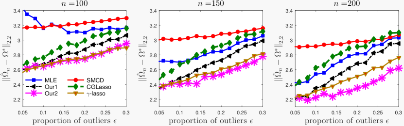
Figure 1: The average error (measured in Frobenius norm) of estimating $\mathbf{\Omega}^{*}$ in Model 1 for $p=30$, when $\epsilon$ is between $5\%$ and $30\%$. Each point is the average of 50 replications.

The third estimator of the precision matrix is obtained by solving an optimization problem whose cost function depends on a robust estimate of the covariance matrix. Two versions of this approach are particularly interesting: the maximum log-likelihood with $\ell_{1}$-penalization known as graphical lasso (d’Aspremont et al., 2008; Banerjee et al., 2008; Friedman et al., 2008) and the constrained $\ell_{1}$-minimization for inverse matrix estimation (CLIME) of Cai et al. (2011). Robust versions of these estimators have been proposed by Öllerer and Croux (2015) and Tarr et al. (2015) and further investigated by Loh and Tan (2015). In this approach, robust estimates of the covariance matrix are plugged-in the graphical lasso or CLIME estimators. In our experiments, the quality of these two versions were comparable. Therefore, we report only the results for the version based on the graphical lasso. In (Öllerer and Croux, 2015), the authors proposed an enhancement that simplifies the estimator and reduces the computational cost, by estimating aside the variances and the correlations. Following their work, we chose to estimate the correlations by the robust Gaussian rank correlation (Boudt et al., 2012) and adopted their implementation choices. In particular, as a robust measure of scale, we used the $Q_{n}$ estimator of Rousseeuw and Croux (1993) that is an alternative to the median absolute deviation (MAD). To sum up, we implemented the correlation based precision matrix estimator obtained by plugging-in the covariance matrix estimate based on pairwise correlations in the graphical lasso (hereinafter referred to as CGLASSO).

The fourth estimator used in our experiments is the $\gamma$-LASSO proposed by Hirose and Fujisawa (2015). The crux of the method is the replacement of the penalized negative log-likelihood function by the penalized negative $\gamma$-likelihood function (Fujisawa and Eguchi, 2008; Cichocki and Amari, 2010). We used the R package rsggm developed by the Hirose and Fujisawa (2015).

Finally we considered two version of our approach, referred to as Our1 and Our2. The first version merely provided by (4) and (5), while the second version consists in re-estimating the precision matrix by the maximum likelihood after removing the observations classified as outliers.

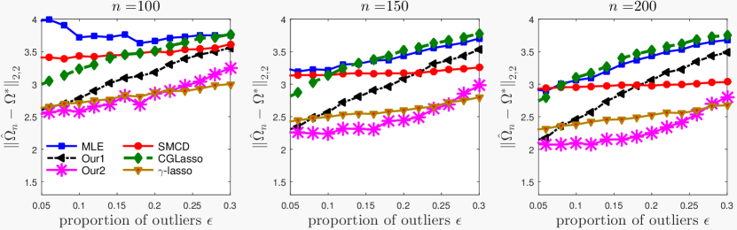
Figure 2: The average error (measured in Frobenius norm) of estimating $\mathbf{\Omega}^{*}$ in Model 2 for $p=30$, when $\epsilon$ is between $5\%$ and $30\%$. Each point is the average of 50 replications.

5.4 Results

The results of our experiments are depicted in Figures 1-4. In all the experiments, the the dimension $p$ is equal to 30 and the contamination rate, denoted by $\epsilon$, is between $5\%$ and $30\%$. The results show that our procedure is competitive with the state-of-the-art robust estimators of the precision matrix, even when the proportion of outliers is high. The results for dimensions $p=10,50,100$ were very similar and therefore are not included in the manuscript.

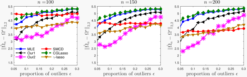
Figure 3: The average error (measured in Frobenius norm) of estimating $\mathbf{\Omega}^{*}$ in Model 3 for $p=30$, when $\epsilon$ is between $5\%$ and $30\%$. Each point is the average of 50 replications.

One may observe that the step of re-estimation of the precision matrix after the removal of the observations classified as outliers reduces the error of estimation in all the considered situations. We would also like to mention that the $\gamma$-lasso, which has a highly competitive statistical accuracy is defined as the minimizer of a nonconvex cost function. Furthermore, there is no theoretical guarantee ensuring the convergence of the algorithm or controlling its statistical error.

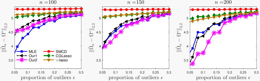
Figure 4: The average error (measured in Frobenius norm) of estimating $\mathbf{\Omega}^{*}$ in Model 4 for $p=30$, when $\epsilon$ is between $5\%$ and $30\%$. Each point is the average of 50 replications.

Supplementary Material

Proofs in high dimension

In this section, we provide the proof of the risk bound in the high dimensional case, when the estimator is obtained by solving the optimization problem in (4). We define ${\mathcal{O}}=O\times[p]$ and, by a slight abuse of notation, ${\mathcal{O}}^{c}=O^{c}\times[p]$. We denote by $\boldsymbol{\xi}_{{\mathcal{O}}}$, resp. $\boldsymbol{\xi}_{{\mathcal{O}}^{c}}$, the matrix obtained by zeroing all the rows $\boldsymbol{\xi}_{i,\bullet}$ such that $i\in O$, resp. $i\in O^{c}$. We set $\bar{\mathbf{\Theta}}^{*}=\mathbf{\Theta}^{*}+\boldsymbol{\xi}_{{\mathcal{O}}}$ and $\bar{\boldsymbol{\xi}}=\boldsymbol{\xi}_{{\mathcal{O}}^{c}}$. We further define $\widehat{\mathbf{\Delta}}^{\mathbf{B}}=\widehat{\mathbf{B}}-{\mathbf{B}}^{*}$, $\widehat{\mathbf{\Delta}}^{\mathbf{\Theta}}=\widehat{\mathbf{\Theta}}-\bar{\mathbf{\Theta}}^{*}$, $\widehat{\mathbf{\Delta}}=\begin{bmatrix}\widehat{\mathbf{\Delta}}^{\mathbf{B}}\\ \widehat{\mathbf{\Delta}}^{\mathbf{\Theta}}\end{bmatrix}\in\mathbb{R}^{(p+n)\times p}$ and $\widehat{\boldsymbol{\xi}}={\mathbf{X}}^{(n)}\widehat{\mathbf{B}}-\widehat{\mathbf{\Theta}}$. Since ${\mathbf{M}}=[{\mathbf{X}}^{(n)};-{\mathbf{I}}_{n}]$, the estimator $(\widehat{\mathbf{B}},\widehat{\mathbf{\Theta}})$ is defined as the minimizer of the cost function

$$F({\mathbf{B}},\mathbf{\Theta})={\bigg{\|}\bigg{(}{\mathbf{M}}\begin{bmatrix}{\mathbf{B}}\\ \mathbf{\Theta}\end{bmatrix}\bigg{)}^{\top}\bigg{\|}}_{2,1}+\lambda\big{(}{\|\mathbf{\Theta}\|}_{2,1}+\gamma{\|{\mathbf{B}}\|}_{1,1}\big{)}.$$

Recall that ${\mathcal{J}}$ and $O$ are such that ${\mathbf{B}}^{*}_{{\mathcal{J}}^{c}}=0$ and $\mathbf{\Theta}^{*}_{O^{c},\bullet}=0$. This sets are interpreted as the supports of ${\mathbf{B}}^{*}$ and $\mathbf{\Theta}^{*}$. The set ${\mathcal{J}}$ corresponds to the sparsity pattern and $O$ to the outliers. Throughout this section, we adopt the convention that $0/0=0$.

Proposition 2.

If, for some constant $c>1$, the penalty levels $\lambda$ and $\gamma$ satisfy the conditions

$$\lambda\gamma\geq\frac{c+1}{c-1}\max_{j\in[p]}\frac{\|{\mathbf{X}}^{(n)}_{I,j^{c}}{}^{\top}\boldsymbol{\epsilon}_{I,j}\|_{\infty}}{{\|\boldsymbol{\epsilon}_{I,j}\|}_{2}}\quad\text{and}\quad\lambda\geq\frac{c+1}{c-1}\max_{i\in[n]}\bigg{(}\sum_{j\in[p]}\frac{\epsilon_{ij}^{2}}{{\|\boldsymbol{\epsilon}_{I,j}\|}_{2}^{2}}\bigg{)}^{1/2},$$ (46)

then the matrix $\widehat{\mathbf{\Delta}}$ belongs to the cone $\mathscr{C}_{{\mathcal{J}},O}(c,\gamma)$.

Proof.

Let us define $\widehat{\boldsymbol{\xi}}$ as the $n\times p$ matrix of estimated residuals: $\widehat{\boldsymbol{\xi}}={\mathbf{X}}^{(n)}\widehat{\mathbf{B}}-\widehat{\mathbf{\Theta}}$. By definition of $\widehat{\mathbf{B}}$ and $\widehat{\mathbf{\Theta}}$, we obtain the inequality

$${\|({\mathbf{X}}^{(n)}\widehat{\mathbf{B}}-\widehat{\mathbf{\Theta}})^{\top}\|}_{2,1}+\lambda\big{(}\gamma{\|\widehat{\mathbf{B}}\|}_{1,1}+{\|\widehat{\mathbf{\Theta}}\|}_{2,1}\big{)} \leq{\|({\mathbf{X}}^{(n)}{\mathbf{B}}^{*}-\bar{\mathbf{\Theta}}^{*})^{\top}\|}_{2,1}+\lambda\big{(}\gamma{\|{\mathbf{B}}^{*}\|}_{1,1}+{\|\bar{\mathbf{\Theta}}^{*}\|}_{2,1}\big{)},$$

that can be equivalently written as

$${\|\widehat{\boldsymbol{\xi}}{}^{\top}\|}_{2,1}+\lambda\gamma{\|\widehat{\mathbf{B}}\|}_{1,1}+\lambda{\|\widehat{\mathbf{\Theta}}\|}_{2,1}\leq{\|\bar{\boldsymbol{\xi}}^{\top}\|}_{2,1}+\lambda\gamma{\|{\mathbf{B}}^{*}\|}_{1,1}+\lambda{\|\bar{\mathbf{\Theta}}^{*}\|}_{2,1},$$

or as

$$\lambda\gamma({\|\widehat{\mathbf{B}}\|}_{1,1}-{\|{\mathbf{B}}^{*}\|}_{1,1})+\lambda({\|\widehat{\mathbf{\Theta}}\|}_{2,1}-{\|\bar{\mathbf{\Theta}}^{*}\|}_{2,1})\leq\sum_{j\in[p]}({\|\bar{\boldsymbol{\xi}}_{\bullet,j}\|}_{2}-{\|\widehat{\boldsymbol{\xi}}_{\bullet,j}\|}_{2}).$$ (47)

In view of the inequality $\|a\|_{2}-\|b\|_{2}\leq(a-b)^{\top}a/\|a\|_{2}$, which holds for every pair of vectors $(a,b)$ and is a simple consequence of the Cauchy-Schwarz inequality, we have

$${\|\bar{\boldsymbol{\xi}}_{\bullet,j}\|}_{2}-{\|\widehat{\boldsymbol{\xi}}_{\bullet,j}\|}_{2} \leq(\boldsymbol{\xi}_{I,j}-\widehat{\boldsymbol{\xi}}_{I,j})^{\top}\frac{\boldsymbol{\xi}_{I,j}}{\|\boldsymbol{\xi}_{I,j}\|_{2}}$$

$$=(\boldsymbol{\xi}_{I,j}-\widehat{\boldsymbol{\xi}}_{I,j})^{\top}\frac{\boldsymbol{\epsilon}_{I,j}}{\|\boldsymbol{\epsilon}_{I,j}\|_{2}}$$

$$=(-{\mathbf{X}}_{I,\bullet}^{(n)}\widehat{\mathbf{\Delta}}^{\mathbf{B}}_{\bullet,j}+\widehat{\mathbf{\Delta}}^{\mathbf{\Theta}}_{I,j})^{\top}\frac{\boldsymbol{\epsilon}_{I,j}}{\|\boldsymbol{\epsilon}_{I,j}\|_{2}}.$$

Summing these inequalities over all $j\in[p]$ and applying the duality inequalities we infer that

$$\sum_{j\in[p]}({\|\boldsymbol{\xi}_{\bullet,j}\|}_{2}-{\|\widehat{\boldsymbol{\xi}}_{\bullet,j}\|}_{2}) \leq-\sum_{j\in[p]}({\mathbf{X}}_{I,\bullet}^{(n)}\widehat{\mathbf{\Delta}}^{{\mathbf{B}}}_{\bullet,j})^{\top}\frac{\boldsymbol{\epsilon}_{I,j}}{\|\boldsymbol{\epsilon}_{I,j}\|_{2}}+\sum_{i\in I}\sum_{j\in[p]}\widehat{\mathbf{\Delta}}^{\mathbf{\Theta}}_{i,j}\frac{\boldsymbol{\epsilon}_{i,j}}{\|\boldsymbol{\epsilon}_{I,j}\|_{2}}$$

$$\leq\sum_{j\in[p]}\|\widehat{\mathbf{\Delta}}^{{\mathbf{B}}}_{\bullet,j}\|_{1}\frac{\|{\mathbf{X}}_{I,j^{c}}^{(n)}{}^{\top}\boldsymbol{\epsilon}_{I,j}\|_{\infty}}{\|\boldsymbol{\epsilon}_{I,j}\|_{2}}+\sum_{i\in[n]}\|\widehat{\mathbf{\Delta}}^{\mathbf{\Theta}}_{i,\bullet}\|_{2}\bigg{(}\sum_{j\in[p]}\frac{\epsilon_{ij}^{2}}{\|\boldsymbol{\epsilon}_{I,j}\|_{2}^{2}}\bigg{)}^{1/2}.$$

When condition (46) is satisfied, the last inequality yields

$$\sum_{j\in[p]}({\|\bar{\boldsymbol{\xi}}_{\bullet,j}\|}_{2}-{\|\widehat{\boldsymbol{\xi}}_{\bullet,j}\|}_{2}) \leq\bigg{(}\frac{c-1}{c+1}\bigg{)}\bigg{(}\lambda\gamma\sum_{j\in[p]}\|\widehat{\mathbf{\Delta}}^{{\mathbf{B}}}_{\bullet,j}\|_{1}+\lambda\sum_{i\in[n]}\|\widehat{\mathbf{\Delta}}^{\mathbf{\Theta}}_{i,\bullet}\|_{2}\bigg{)}$$

$$=\lambda\bigg{(}\frac{c-1}{c+1}\bigg{)}\big{(}\gamma\|\widehat{\mathbf{\Delta}}^{{\mathbf{B}}}\|_{1,1}+\|\widehat{\mathbf{\Delta}}^{\mathbf{\Theta}}\|_{2,1}\big{)}.$$

This inequality, in conjunction with Eq. (47), implies that

$$\gamma({\|\widehat{\mathbf{B}}\|}_{1,1}-{\|{\mathbf{B}}^{*}\|}_{1,1})+({\|\widehat{\mathbf{\Theta}}\|}_{2,1}-{\|\bar{\mathbf{\Theta}}^{*}\|}_{2,1})\leq\bigg{(}\frac{c-1}{c+1}\bigg{)}\big{(}\gamma\|\widehat{\mathbf{\Delta}}^{{\mathbf{B}}}\|_{1,1}+\|\widehat{\mathbf{\Delta}}^{\mathbf{\Theta}}\|_{2,1}\big{)}.$$ (48)

On the other hand, using the triangle inequality and the fact that ${\mathbf{B}}_{{\mathcal{J}}^{c}}^{*}=\mathbf{\Theta}_{O^{c},\bullet}^{*}=0$, we get

$${\|\widehat{\mathbf{B}}\|}_{1,1}-{\|{\mathbf{B}}^{*}\|}_{1,1} ={\|\widehat{\mathbf{B}}_{{\mathcal{J}}^{c}}\|}_{1,1}+{\|\widehat{\mathbf{B}}_{{\mathcal{J}}}\|}_{1,1}-{\|{\mathbf{B}}^{*}_{{\mathcal{J}}}\|}_{1,1}$$

$$\geq{\|\widehat{\mathbf{\Delta}}^{{\mathbf{B}}}_{{\mathcal{J}}^{c}}\|}_{1,1}-{\|\widehat{\mathbf{\Delta}}^{\mathbf{B}}_{{\mathcal{J}}}\|}_{1,1},$$

$${\|\widehat{\mathbf{\Theta}}\|}_{2,1}-{\|\bar{\mathbf{\Theta}}^{*}\|}_{2,1} ={\|\widehat{\mathbf{\Theta}}_{O^{c},\bullet}\|}_{2,1}+{\|\widehat{\mathbf{\Theta}}_{O,\bullet}\|}_{2,1}-{\|\bar{\mathbf{\Theta}}^{*}_{O,\bullet}\|}_{2,1}$$

$$\geq{\|\widehat{\mathbf{\Delta}}^{\mathbf{\Theta}}_{O^{c},\bullet}\|}_{2,1}-{\|\widehat{\mathbf{\Delta}}^{\mathbf{\Theta}}_{O,\bullet}\|}_{2,1}.$$

The combination of these bounds with Eq. (48) leads to

$${\|\widehat{\mathbf{\Delta}}^{\mathbf{B}}_{{\mathcal{J}}^{c}}\|}_{1,1}+\gamma^{-1}{\|\widehat{\mathbf{\Delta}}^{\mathbf{\Theta}}_{O^{c},\bullet}\|}_{2,1} \leq c\big{(}{\|\widehat{\mathbf{\Delta}}^{\mathbf{B}}_{{\mathcal{J}}}\|}_{1,1}+\gamma^{-1}{\|\widehat{\mathbf{\Delta}}^{\mathbf{\Theta}}_{O,\bullet}\|}_{2,1}\big{)},$$

which completes the proof of the proposition. ∎

The following lemmas prepare the proof of Theorem 3. Lemma 13 presents an inequality obtained by writing the KKT conditions for the cost function $F$.

Lemma 13.

There exists a $n\times p$ matrix ${\mathbf{V}}$ is such that

$$\|{\mathbf{V}}_{i,\bullet}\|_{2}\leq 1,\qquad{\mathbf{V}}_{i,\bullet}^{\top}\widehat{\mathbf{\Theta}}_{i,\bullet}=\|\widehat{\mathbf{\Theta}}_{i,\bullet}\|_{2},\qquad\forall\,i\in[n]$$ (49)

and, for every $j\in[p]$ such that $\widehat{\boldsymbol{\xi}}_{\bullet,j}\neq 0$, the following inequality holds

$${\|{\mathbf{M}}\widehat{\mathbf{\Delta}}_{\bullet,j}\|}_{2}^{2} \leq-\bar{\boldsymbol{\xi}}_{\bullet,j}^{\top}{\mathbf{M}}\widehat{\mathbf{\Delta}}_{\bullet,j}-\lambda{\|\widehat{\boldsymbol{\xi}}_{\bullet,j}\|}_{2}{\mathbf{V}}_{\bullet,j}^{\top}\widehat{\mathbf{\Delta}}^{\mathbf{\Theta}}_{\bullet,j}+\lambda\gamma{\|\widehat{\xi}_{\bullet,j}\|}_{2}\big{(}{\|{\mathbf{B}}^{*}_{j^{c},j}\|}_{1}-{\|\widehat{\mathbf{B}}_{j^{c},j}\|}_{1}\big{)}.$$ (50)

Proof.

Recall that the estimator $(\widehat{\mathbf{B}},\widehat{\mathbf{\Theta}})$ minimizes the cost function

$$F({\mathbf{B}},\mathbf{\Theta})=\sum_{j=1}^{p}{\|{\mathbf{X}}^{(n)}_{\bullet,j}+{\mathbf{X}}^{(n)}_{\bullet,j^{c}}{\mathbf{B}}_{j^{c},j}-\mathbf{\Theta}_{\bullet,j}\|}_{2}+\lambda\gamma\sum_{j=1}^{p}{\|{\mathbf{B}}_{\bullet,j}\|}_{1}+\lambda\sum_{i=1}^{n}{\|\mathbf{\Theta}_{i,\bullet}\|}_{2}.$$ (51)

According to the KKT conditions, this convex function is minimized at $(\widehat{\mathbf{B}},\widehat{\mathbf{\Theta}})$ if and only if the zero vector belongs to the sub-differential of $F$ at $(\widehat{\mathbf{B}},\widehat{\mathbf{\Theta}})$, denoted by $\partial F(\widehat{\mathbf{B}},\widehat{\mathbf{\Theta}})$. This entails, in particular, that for every $j\in[p]$, $\mathbf{0}_{p-1+n}\in\partial_{({\mathbf{B}}_{j^{c},j},\mathbf{\Theta}_{\bullet,j})}F(\widehat{\mathbf{B}},\widehat{\mathbf{\Theta}})$. In other terms, there exist vectors ${\mathbf{u}}_{j}\in\partial_{({\mathbf{B}}_{j^{c},j},\mathbf{\Theta}_{\bullet,j})}{\|{\mathbf{X}}^{(n)}_{\bullet,j}+{\mathbf{X}}^{(n)}_{\bullet,j^{c}}\widehat{\mathbf{B}}_{j^{c},j}-\widehat{\mathbf{\Theta}}_{\bullet,j}\|}_{2}$, ${\mathbf{w}}_{j}\in\partial_{({\mathbf{B}}_{j^{c},j},\mathbf{\Theta}_{\bullet,j})}{\|\widehat{\mathbf{B}}_{\bullet,j}\|}_{1}$ and ${\mathbf{v}}_{j}\in\partial_{({\mathbf{B}}_{j^{c},j},\mathbf{\Theta}_{\bullet,j})}\sum_{i=1}^{n}{\|\widehat{\mathbf{\Theta}}_{i,\bullet}\|}_{2}$ such that ${\mathbf{u}}_{j}+\lambda\gamma{\mathbf{w}}_{j}+\lambda{\mathbf{v}}_{j}=0$. Since we assume that ${\|\widehat{\boldsymbol{\xi}}_{\bullet,j}\|}_{2}>0$, the first partial sub-differential out of three appearing in the previous sentence is actually a differential and thus ${\mathbf{u}}_{j}=[{\mathbf{X}}^{(n)}_{\bullet,j^{c}};-{\mathbf{I}}_{n}]^{\top}({\mathbf{X}}^{(n)}\widehat{\mathbf{B}}_{\bullet,j}-\widehat{\mathbf{\Theta}}_{\bullet,j})/{\|\widehat{\boldsymbol{\xi}}_{\bullet,j}\|}_{2}$. After a multiplication by ${\|\widehat{\boldsymbol{\xi}}_{\bullet,j}\|}_{2}$, we get

$$[{\mathbf{X}}^{(n)}_{\bullet,j^{c}};-{\mathbf{I}}_{n}]^{\top}({\mathbf{X}}^{(n)}\widehat{\mathbf{B}}_{\bullet,j}-\widehat{\mathbf{\Theta}}_{\bullet,j})=-\lambda\gamma{\|\widehat{\boldsymbol{\xi}}_{\bullet,j}\|}_{2}{\mathbf{w}}_{j}-\lambda{\|\widehat{\boldsymbol{\xi}}_{\bullet,j}\|}_{2}{\mathbf{v}}_{j}.$$

This equation (combined with relation (8)) can be equivalently written as

$$[{\mathbf{X}}^{(n)}_{\bullet,j^{c}};-{\mathbf{I}}_{n}]^{\top}{\mathbf{M}}\widehat{\mathbf{\Delta}}_{\bullet,j}=-[{\mathbf{X}}^{(n)}_{\bullet,j^{c}};-{\mathbf{I}}_{n}]^{\top}\bar{\boldsymbol{\xi}}_{\bullet,j}-\lambda\gamma{\|\widehat{\boldsymbol{\xi}}_{\bullet,j}\|}_{2}{\mathbf{w}}_{j}-\lambda{\|\widehat{\boldsymbol{\xi}}_{\bullet,j}\|}_{2}{\mathbf{v}}_{j}.$$

We take the scalar product of the both sides of this relation with the vector $\widehat{\mathbf{\Delta}}_{j^{c},j}$ and, using the fact that $\widehat{\mathbf{\Delta}}_{j,j}=0$, we obtain

$$\|{\mathbf{M}}\widehat{\mathbf{\Delta}}_{\bullet,j}\|_{2}^{2}=-\widehat{\mathbf{\Delta}}_{\bullet,j}^{\top}{\mathbf{M}}^{\top}\bar{\boldsymbol{\xi}}_{\bullet,j}-\lambda\gamma{\|\widehat{\boldsymbol{\xi}}_{\bullet,j}\|}_{2}\widehat{\mathbf{\Delta}}_{\bullet,j}^{\top}{\mathbf{w}}_{j}-\lambda{\|\widehat{\boldsymbol{\xi}}_{\bullet,j}\|}_{2}\widehat{\mathbf{\Delta}}_{\bullet,j}^{\top}{\mathbf{v}}_{j}.$$

The desired inequality follows by setting ${\mathbf{V}}=[({\mathbf{v}}_{1})_{p:(p-1+n)},\ldots,({\mathbf{v}}_{p})_{p:(p-1+n)}]$ and by using the following simple properties of the sub-differentials of the $\ell_{1}$ and $\ell_{2}$-norms:

$$({\mathbf{w}}_{j})_{l} =0,\qquad\forall l\geq p,$$

$$|({\mathbf{w}}_{j})_{l}| \leq 1,\qquad\forall l\in[p-1],$$

$$({\mathbf{w}}_{j})_{1:(p-1)}^{\top} \widehat{\mathbf{B}}_{j^{c},j}=\|\widehat{\mathbf{B}}_{j^{c},j}\|_{1},$$

$$({\mathbf{v}}_{j})_{l} =0,\qquad\forall l\in[p-1],$$

$$({\mathbf{v}}_{j})_{p-1+i} =\frac{\widehat{\mathbf{\Theta}}_{i,j}}{\|\widehat{\mathbf{\Theta}}_{i,\bullet}\|_{2}},\qquad\begin{cases}i\in[n],\\ \|\widehat{\mathbf{\Theta}}_{i,\bullet}\|_{2}>0,\end{cases}$$

$$|({\mathbf{v}}_{j})_{p-1+i}| \leq\frac{|\boldsymbol{\theta}_{j}|}{\|\boldsymbol{\theta}\|_{2}},\qquad\qquad\begin{cases}i\in[n],\\ \|\widehat{\mathbf{\Theta}}_{i,\bullet}\|_{2}=0,\\ \forall\boldsymbol{\theta}\in\mathbb{R}^{p},\|\boldsymbol{\theta}\|_{2}>0.\end{cases}$$

Indeed, the first three relations imply that $-\widehat{\mathbf{\Delta}}_{\bullet,j}^{\top}{\mathbf{w}}_{j}\leq\|{\mathbf{B}}^{*}_{\bullet,j}\|_{1}-\|\widehat{\mathbf{B}}_{\bullet,j}\|_{1}$ while the three last relations yield $\widehat{\mathbf{\Delta}}_{\bullet,j}^{\top}{\mathbf{v}}_{j}={\mathbf{V}}_{\bullet,j}^{\top}\widehat{\mathbf{\Delta}}^{\mathbf{\Theta}}_{\bullet,j}$ along with $\|{\mathbf{V}}_{i,\bullet}\|_{2}\leq 1$ and ${\mathbf{V}}_{i,\bullet}\widehat{\mathbf{\Theta}}_{i,\bullet}^{\top}=\|\widehat{\mathbf{\Theta}}_{i,\bullet}\|_{2}$. ∎

Lemma 14.

If inequality (50) is true, then

$${\|{\mathbf{M}}\widehat{\mathbf{\Delta}}_{\bullet,j}\|}_{2}^{2} \leq-2\bar{\boldsymbol{\xi}}_{\bullet,j}^{\top}{\mathbf{M}}\widehat{\mathbf{\Delta}}_{\bullet,j}-2\lambda{\|\bar{\boldsymbol{\xi}}_{\bullet,j}\|}_{2}{\mathbf{V}}_{\bullet,j}^{\top}\widehat{\mathbf{\Delta}}^{\mathbf{\Theta}}_{\bullet,j}+2\lambda\gamma{\|\bar{\boldsymbol{\xi}}_{\bullet,j}\|}_{2}\big{(}{\|{\mathbf{B}}^{*}_{j^{c},j}\|}_{1}-{\|\widehat{\mathbf{B}}_{j^{c},j}\|}_{1}\big{)}$$

$$\qquad+\lambda^{2}(\gamma{\|\widehat{\mathbf{\Delta}}_{\bullet,j}^{\mathbf{B}}\|}_{1}+|{\mathbf{V}}_{\bullet,j}^{\top}\widehat{\mathbf{\Delta}}^{\mathbf{\Theta}}_{\bullet,j}|)^{2}.$$ (52)

Proof.

This is a direct consequence of Lemma 3 (with $R={\|{\mathbf{M}}\widehat{\mathbf{\Delta}}_{\bullet,j}\|}_{2}$) and the fact that $|{\|\widehat{\xi}_{\bullet,j}\|}_{2}-{\|\bar{\xi}_{\bullet,j}\|}|_{2}\leq{\|{\mathbf{M}}\widehat{\mathbf{\Delta}}_{\bullet,j}\|}_{2}$. ∎

Lemma 15.

If inequality (14) is true and if the penalty levels $\lambda$ and $\gamma$ satisfy conditions (46) for some constant $c>1$, then

$${\|{\mathbf{M}}\widehat{\mathbf{\Delta}}\|}_{F}^{2} \leq 4\lambda c{\|\boldsymbol{\xi}_{I,\bullet}^{\top}\|}_{2,\infty}\big{(}\gamma{\|\widehat{\mathbf{\Delta}}_{\mathcal{J}}^{\mathbf{B}}\|}_{1,1}+{\|\widehat{\mathbf{\Delta}}_{O,\bullet}^{\mathbf{\Theta}}\|}_{2,1}\big{)}+\lambda^{2}(1+c)^{2}\big{(}\gamma{\|\widehat{\mathbf{\Delta}}_{\mathcal{J}}^{\mathbf{B}}\|}_{1,1}+{\|\widehat{\mathbf{\Delta}}_{O,\bullet}^{\mathbf{\Theta}}\|}_{2,1}\big{)}^{2}.$$ (53)

Proof.

We begin by noting that for a $n\times p$ matrix ${\mathbf{V}}$ that satisfies ${\|{\mathbf{V}}_{i,\bullet}\|}_{2}\leq 1$ for any $i$ belonging to $[n]$, the Cauchy-Schwarz inequality yields that

$$\sum_{j=1}^{p}|{\mathbf{V}}_{\bullet,j}^{\top}\widehat{\mathbf{\Delta}}^{\mathbf{\Theta}}_{\bullet,j}|\leq\sum_{i=1}^{n}\sum_{j=1}^{p}|{\mathbf{V}}_{i,j}\widehat{\mathbf{\Delta}}^{\mathbf{\Theta}}_{i,j}|\leq\sum_{i=1}^{n}{\|{\mathbf{V}}_{i,\bullet}\|}_{2}{\|\widehat{\mathbf{\Delta}}^{\mathbf{\Theta}}_{i,\bullet}\|}_{2}\leq{\|\widehat{\mathbf{\Delta}}^{\mathbf{\Theta}}\|}_{2,1}.$$ (54)

We also deduce

$$\sum_{j=1}^{p}\big{(}\gamma{\|\widehat{\mathbf{\Delta}}_{\bullet,j}^{\mathbf{B}}\|}_{1}+|{\mathbf{V}}_{\bullet,j}^{\top}\widehat{\mathbf{\Delta}}^{\mathbf{\Theta}}_{\bullet,j}|\big{)}^{2} \leq\Big{(}\sum_{j=1}^{p}\gamma{\|\widehat{\mathbf{\Delta}}_{\bullet,j}^{\mathbf{B}}\|}_{1}+|{\mathbf{V}}_{\bullet,j}^{\top}\widehat{\mathbf{\Delta}}^{\mathbf{\Theta}}_{\bullet,j}|\Big{)}^{2}$$

$$\leq\big{(}\gamma{\|\widehat{\mathbf{\Delta}}^{\mathbf{B}}\|}_{1,1}+{\|\widehat{\mathbf{\Delta}}^{\mathbf{\Theta}}\|}_{2,1}\big{)}^{2}.$$ (55)

Besides, it holds

$$-\sum_{j=1}^{p}\bar{\boldsymbol{\xi}}_{\bullet,j}^{\top}{\mathbf{M}}\widehat{\mathbf{\Delta}}_{\bullet,j} =\sum_{j=1}^{p}\big{(}\widehat{\mathbf{\Delta}}^{\mathbf{\Theta}}_{\bullet,j}-{\mathbf{X}}^{(n)}\widehat{\mathbf{\Delta}}^{\mathbf{B}}_{\bullet,j}\big{)}^{\top}\bar{\boldsymbol{\xi}}_{\bullet,j}$$

$$=\sum_{j=1}^{p}{\|\bar{\boldsymbol{\xi}}_{\bullet,j}\|}_{2}\Big{(}\sum_{i\in I}\widehat{\mathbf{\Delta}}^{\mathbf{\Theta}}_{i,j}\frac{\boldsymbol{\epsilon}_{i,j}}{{\|\boldsymbol{\epsilon}_{\bullet,j}\|}_{2}}-\widehat{\mathbf{\Delta}}^{\mathbf{B}}_{\bullet,j}{}^{\top}{\mathbf{X}}^{(n)}_{I,\bullet}{}^{\top}\frac{\boldsymbol{\epsilon}_{I,j}}{{\|\boldsymbol{\epsilon}_{I,j}\|}_{2}}\Big{)}$$

$$\leq(\max_{j\in[p]}{\|\boldsymbol{\xi}_{I,j}\|}_{2})\Big{(}\sum_{i\in I}\sum_{j=1}^{p}\frac{|\widehat{\mathbf{\Delta}}^{\mathbf{\Theta}}_{i,j}\boldsymbol{\epsilon}_{i,j}|}{{\|\boldsymbol{\epsilon}_{I,j}\|}_{2}}+\sum_{j=1}^{p}\frac{|\widehat{\mathbf{\Delta}}^{\mathbf{B}}_{\bullet,j}{}^{\top}{\mathbf{X}}^{(n)}_{I,\bullet}{}^{\top}\boldsymbol{\epsilon}_{I,j}|}{{\|\boldsymbol{\epsilon}_{I,j}\|}_{2}}\Big{)},$$

thus, by the duality inequality $|\widehat{\mathbf{\Delta}}^{\mathbf{B}}_{\bullet,j}{}^{\top}{\mathbf{X}}^{(n)}_{I,\bullet}{}^{\top}\boldsymbol{\epsilon}_{I,j}|\leq{\|\widehat{\mathbf{\Delta}}^{\mathbf{B}}_{\bullet,j}\|}_{1}{\|{\mathbf{X}}^{(n)}_{I,\bullet}{}^{\top}\boldsymbol{\epsilon}_{I,j}\|}_{\infty}$ and the Cauchy-Schwarz inequality, and as the penalty levels satisfy conditions (46), we find

$$-\sum_{j=1}^{p}\bar{\boldsymbol{\xi}}_{\bullet,j}^{\top}{\mathbf{M}}\widehat{\mathbf{\Delta}}_{\bullet,j} \leq{\|\boldsymbol{\xi}_{I,\bullet}^{\top}\|}_{2,\infty}\Big{(}\sum_{i\in I}{\|\widehat{\mathbf{\Delta}}^{\mathbf{\Theta}}_{i,\bullet}\|}_{2}\Big{(}\sum_{j=1}^{p}\frac{\boldsymbol{\epsilon}_{i,j}^{2}}{{\|\boldsymbol{\epsilon}_{I,j}\|}_{2}^{2}}\Big{)}^{\frac{1}{2}}+\sum_{j=1}^{p}{\|\widehat{\mathbf{\Delta}}^{\mathbf{B}}_{\bullet,j}\|}_{1}\frac{{\|{\mathbf{X}}^{(n)}_{I,\bullet}{}^{\top}\boldsymbol{\epsilon}_{I,j}\|}_{\infty}}{{\|\boldsymbol{\epsilon}_{I,j}\|}_{2}}\Big{)}$$

$$\leq\lambda\frac{c-1}{c+1}\big{(}\gamma{\|\widehat{\mathbf{\Delta}}^{\mathbf{B}}\|}_{1,1}+{\|\widehat{\mathbf{\Delta}}^{\mathbf{\Theta}}\|}_{2,1}\big{)}{\|\boldsymbol{\xi}_{I,\bullet}^{\top}\|}_{2,\infty}.$$ (56)

From inequality (14), we get

$${\|{\mathbf{M}}\widehat{\mathbf{\Delta}}_{\bullet,j}\|}_{2}^{2} \leq-2\bar{\boldsymbol{\xi}}_{\bullet,j}^{\top}{\mathbf{M}}\widehat{\mathbf{\Delta}}_{\bullet,j}-2\lambda{\|\bar{\boldsymbol{\xi}}_{\bullet,j}\|}_{2}\Big{(}{\mathbf{V}}_{\bullet,j}^{\top}\widehat{\mathbf{\Delta}}^{\mathbf{\Theta}}_{\bullet,j}+\gamma\big{(}{\|\widehat{\mathbf{B}}_{j^{c},j}\|}_{1}-{\|{\mathbf{B}}^{*}_{j^{c},j}\|}_{1}\big{)}\Big{)}$$

$$\qquad+\lambda^{2}\big{(}\gamma{\|\widehat{\mathbf{\Delta}}_{\bullet,j}^{\mathbf{B}}\|}_{1}+|{\mathbf{V}}_{\bullet,j}^{\top}\widehat{\mathbf{\Delta}}^{\mathbf{\Theta}}_{\bullet,j}|\big{)}^{2},$$

for every $j\in[p]$. Then, summing over all $j$ and using the triangle inequality, we have

$${\|{\mathbf{M}}\widehat{\mathbf{\Delta}}\|}_{F}^{2} \leq-2\sum_{j=1}^{p}\bar{\boldsymbol{\xi}}_{\bullet,j}^{\top}{\mathbf{M}}\widehat{\mathbf{\Delta}}_{\bullet,j}+2\lambda{\|\boldsymbol{\xi}_{I,j}\|}_{2}\Big{(}|{\mathbf{V}}_{\bullet,j}^{\top}\widehat{\mathbf{\Delta}}^{\mathbf{\Theta}}_{\bullet,j}|+\gamma{\|\widehat{\mathbf{\Delta}}_{\bullet,j}^{\mathbf{B}}\|}_{1}\Big{)}$$

$$\qquad+\lambda^{2}\big{(}\gamma{\|\widehat{\mathbf{\Delta}}_{\bullet,j}^{\mathbf{B}}\|}_{1}+|{\mathbf{V}}_{\bullet,j}^{\top}\widehat{\mathbf{\Delta}}^{\mathbf{\Theta}}_{\bullet,j}|\big{)}^{2}.$$

Combining the latter with equations (54), (55) and (56), we arrive at

$${\|{\mathbf{M}}\widehat{\mathbf{\Delta}}\|}_{F}^{2} \leq\lambda\frac{4c}{c+1}\big{(}\gamma{\|\widehat{\mathbf{\Delta}}^{\mathbf{B}}\|}_{1,1}+{\|\widehat{\mathbf{\Delta}}^{\mathbf{\Theta}}\|}_{2,1}\big{)}{\|\boldsymbol{\xi}_{I,\bullet}^{\top}\|}_{2,\infty}+\lambda^{2}\big{(}\gamma{\|\widehat{\mathbf{\Delta}}^{\mathbf{B}}\|}_{1,1}+{\|\widehat{\mathbf{\Delta}}^{\mathbf{\Theta}}\|}_{2,1}\big{)}^{2},$$

we finally apply Proposition 2 that gives inequality (53). ∎

Proposition 3.

Choose $\gamma=1$ and $\delta\in(0,1)$ such that $n\geq|O|+16\log(2p/\delta)$ and choose

$$\lambda=6\bigg{(}\frac{\log(2np/\delta)}{n-|O|}\bigg{)}^{1/2}.$$ (57)

Then

1. with probability at least $1-\delta$, the penalty levels $\lambda$ and $\gamma$ satisfy conditions (46) for some constant $c=2$.

2. If $4\lambda(|{\mathcal{J}}|^{1/2}+|O|^{1/2})<\kappa^{1/2}$ holds, then there exists an event $\mathcal{E}_{0}$ of probability at least $1-2\delta$ such that in $\mathcal{E}_{\kappa}\cap\mathcal{E}_{0}$, we have

   $${\|{\mathbf{M}}\widehat{\mathbf{\Delta}}\|}_{2,2} \leq\frac{C_{2}}{\sqrt{\kappa}}\max_{j\in[p]}(\omega^{*}_{jj})^{-1/2}\big{(}|{\mathcal{J}}|^{1/2}+|O|^{1/2}\big{)}\bigg{(}\frac{\log(2np/\delta)}{n-|O|}\bigg{)}^{1/2},$$ (58)

   $${\|\widehat{\mathbf{\Delta}}^{\mathbf{B}}\|}_{1,1} +{\|\widehat{\mathbf{\Delta}}^{\mathbf{\Theta}}\|}_{2,1}\leq\frac{12C_{2}}{\kappa}\max_{j\in[p]}(\omega^{*}_{jj})^{-1/2}\big{(}|{\mathcal{J}}|+|O|\big{)}\bigg{(}\frac{\log(2np/\delta)}{n-|O|}\bigg{)}^{1/2}$$ (59)

   with $C_{2}\leq 75$.

Proof.

Claim i) of the proposition is obtained by standard arguments relying on tail bounds for Gaussian and $\chi^{2}$ distributions and the union bound. These arguments are similar to those presented in Section 4.3 and, therefore, are skipped.

Analogously, using Lemma 12, we find that with probability at least $1-\delta$, we have $\|\boldsymbol{\xi}_{I,\bullet}\|_{2,\infty}\leq(1+2^{-3/2})\max_{j}(\omega_{jj}^{*})^{-1/2}$. We denote by $\mathcal{E}_{0}$ the intersection of this event with the one of claim i). By the union bound, we have ${\mathbf{P}}(\mathcal{E}_{0})\geq 1-2\delta$. In the rest of this proof, we place ourselves in the vent $\mathcal{E}_{0}\cap\mathcal{E}_{\kappa}$. By the compatibility assumption (event $\mathcal{E}_{\kappa}$), we have

$${\|\widehat{\mathbf{\Delta}}_{\mathcal{J}}^{\mathbf{B}}\|}_{1,1}\leq\frac{|{\mathcal{J}}|^{1/2}}{\kappa^{1/2}}{\|{\mathbf{M}}\widehat{\mathbf{\Delta}}\|}_{2,2}\quad\text{and}\quad{\|\widehat{\mathbf{\Delta}}_{O,\bullet}^{\mathbf{\Theta}}\|}_{2,1}\leq\frac{|O|^{1/2}}{\kappa^{1/2}}{\|{\mathbf{M}}\widehat{\mathbf{\Delta}}\|}_{2,2}.$$ (60)

Since in the event $\mathcal{E}_{0}$ the conditions of Lemma 15 are met, inequality (53) readily implies inequality (58). On the other hand, we know from Proposition 2 that $\widehat{\mathbf{\Delta}}$ belongs to the dimension reduction cone $\mathscr{C}_{{\mathcal{J}},O}(2,1)$. Therefore,

$${\|\widehat{\mathbf{\Delta}}^{\mathbf{B}}\|}_{1,1}+{\|\widehat{\mathbf{\Delta}}^{\mathbf{\Theta}}\|}_{2,1}\leq 3({\|\widehat{\mathbf{\Delta}}_{\mathcal{J}}^{\mathbf{B}}\|}_{1,1}+{\|\widehat{\mathbf{\Delta}}_{O,\bullet}^{\mathbf{\Theta}}\|}_{2,1})\leq\frac{3(|{\mathcal{J}}|\vee|O|)^{1/2}}{\kappa^{1/2}}{\|{\mathbf{M}}\widehat{\mathbf{\Delta}}\|}_{2,2}.$$

Using the upper bound on ${\|{\mathbf{M}}\widehat{\mathbf{\Delta}}\|}_{2,2}$ provided by (58), we immediately obtain bound (59). ∎

References

- Banerjee et al. (2008) O. Banerjee, L. El Ghaoui, and A. d’Aspremont. Model selection through sparse maximum likelihood estimation for multivariate Gaussian or binary data. J. Mach. Learn. Res., 9:485–516, June 2008.
- Belloni et al. (2011) A. Belloni, V. Chernozhukov, and L. Wang. Square-root Lasso: pivotal recovery of sparse signals via conic programming. Biometrika, 98(4):791–806, December 2011.
- Bickel et al. (2009) P. J. Bickel, Y. Ritov, and A. B. Tsybakov. Simultaneous analysis of Lasso and Dantzig selector. Ann. Statist., 37(4):1705–1732, August 2009.
- Boudt et al. (2012) Kris Boudt, Jonathan Cornelissen, and Christophe Croux. The gaussian rank correlation estimator: robustness properties. Statistics and Computing, 22(2):471–483, 2012.
- Cai et al. (2011) T. Cai, W. Liu, and X. Luo. A Constrained L1 Minimization Approach to Sparse Precision Matrix Estimation. Journal of the American Statistical Association, 106:594–607, February 2011.
- Candès and Randall (2008) Emmanuel J. Candès and Paige A. Randall. Highly robust error correction by convex programming. IEEE Trans. Inform. Theory, 54(7):2829–2840, 2008. ISSN 0018-9448. doi: 10.1109/TIT.2008.924688. URL http://dx.doi.org/10.1109/TIT.2008.924688.
- Chen et al. (2015) M. Chen, C. Gao, and Z. Ren. Robust Covariance Matrix Estimation via Matrix Depth. ArXiv e-prints, June 2015.
- Chen et al. (2015) M. Chen, C. Gao, and Z. Ren. Robust Covariance Matrix Estimation via Matrix Depth. arXiv:1506.00691, 2015.
- Chen et al. (2010) Yilun Chen, A. Wiesel, Y.C. Eldar, and A.O. Hero. Shrinkage algorithms for mmse covariance estimation. Signal Processing, IEEE Transactions on, 58(10):5016–5029, Oct 2010.
- Cichocki and Amari (2010) A. Cichocki and S. Amari. Families of alpha- beta- and gamma- divergences: Flexible and robust measures of similarities. Entropy, 12(6):1532, 2010. URL http://www.mdpi.com/1099-4300/12/6/1532.
- Dalalyan and Keriven (2012) Arnak Dalalyan and Renaud Keriven. Robust estimation for an inverse problem arising in multiview geometry. J. Math. Imaging Vision, 43(1):10–23, 2012.
- Dalalyan and Chen (2012) Arnak S. Dalalyan and Yin Chen. Fused sparsity and robust estimation for linear models with unknown variance. In Advances in Neural Information Processing Systems 25, pages 1268–1276, 2012.
- d’Aspremont et al. (2008) A. d’Aspremont, O. Banerjee, and L. El Ghaoui. First-order methods for sparse covariance selection. SIAM. J. Matrix Anal. & Appl., 30(1):56–66, February 2008.
- Friedman et al. (2008) J. Friedman, T. Hastie, and R. Tibshirani. Sparse inverse covariance estimation with the graphical lasso. Biostatistics, 9(3):432–441, July 2008.
- Fujisawa and Eguchi (2008) H. Fujisawa and S. Eguchi. Robust parameter estimation with a small bias against heavy contamination. J. Multivar. Anal., 99(9):2053–2081, October 2008. ISSN 0047-259X. URL http://dx.doi.org/10.1016/j.jmva.2008.02.004.
- Hampel et al. (1986) Frank R. Hampel, Elvezio M. Ronchetti, Peter J. Rousseeuw, and Werner A. Stahel. Robust statistics. Wiley Series in Probability and Mathematical Statistics: Probability and Mathematical Statistics. John Wiley & Sons, Inc., New York, 1986. The approach based on influence functions.
- Higham (2002) N. J. Higham. Computing the nearest correlation matrix—a problem from finance. IMA journal of Numerical Analysis, 22(3):329–343, 2002.
- Hirose and Fujisawa (2015) K. Hirose and H. Fujisawa. Robust sparse Gaussian graphical modeling. ArXiv e-prints, August 2015. URL http://arxiv.org/abs/1508.05571.
- Huber and Ronchetti (2009) Peter J. Huber and Elvezio M. Ronchetti. Robust statistics. Wiley Series in Probability and Statistics. John Wiley & Sons, Inc., Hoboken, NJ, second edition, 2009.
- Klopp and Tsybakov (2015) O. Klopp and A. B. Tsybakov. Estimation of matrices with row sparsity. ArXiv e-prints, September 2015.
- Klopp et al. (2014) O. Klopp, K. Lounici, and A. B. Tsybakov. Robust Matrix Completion. ArXiv e-prints, December 2014.
- Laurent and Massart (2000) B. Laurent and P. Massart. Adaptive estimation of a quadratic functional by model selection. Ann. Statist., 28(5):1302–1338, October 2000.
- Loh and Tan (2015) P.-L. Loh and X. L. Tan. High-dimensional robust precision matrix estimation: Cellwise corruption under -contamination. ArXiv e-prints, September 2015.
- Lounici et al. (2011) Karim Lounici, Massimiliano Pontil, Sara van de Geer, and Alexandre B. Tsybakov. Oracle inequalities and optimal inference under group sparsity. Ann. Statist., 39(4):2164–2204, 08 2011.
- Maronna et al. (2006) Ricardo A. Maronna, Douglas R. Martin, and Victor J. Yohai. Robust Statistics: Theory and Methods. John Wiley and Sons, New York, 2006.
- Nguyen and Tran (2013) Nam H. Nguyen and Trac D. Tran. Robust Lasso with missing and grossly corrupted observations. IEEE Trans. Inform. Theory, 59(4):2036–2058, 2013.
- Öllerer and Croux (2015) V. Öllerer and C. Croux. Robust high-dimensional precision matrix estimation. ArXiv e-prints, January 2015.
- Raskutti et al. (2010) G. Raskutti, M. J. Wainwright, and B. Yu. Restricted eigenvalue properties for correlated Gaussian designs. J. Mach. Learn. Res., 11:2241–2259, August 2010.
- Rousseeuw (1984) Peter J Rousseeuw. Least median of squares regression. Journal of the American statistical association, 79(388):871–880, 1984.
- Rousseeuw (1985) Peter J Rousseeuw. Multivariate estimation with high breakdown point. Mathematical Statistics and Applications, 8:283–297, 1985.
- Rousseeuw and Croux (1993) Peter J Rousseeuw and Christophe Croux. Alternatives to the median absolute deviation. Journal of the American Statistical association, 88(424):1273–1283, 1993.
- Sun and Zhang (2012) T. Sun and C-H. Zhang. Scaled sparse linear regression. Biometrika, 99(4):879–898, September 2012.
- Sun and Zhang (2013) T. Sun and C-H. Zhang. Sparse matrix inversion with scaled Lasso. J. Mach. Learn. Res., 14:3385–3418, November 2013.
- Tarr et al. (2015) G. Tarr, S. Müller, and N. C. Weber. Robust estimation of precision matrices under cellwise contamination. ArXiv e-prints, January 2015.
- Vershynin (2012) R. Vershynin. Introduction to the non-asymptotic analysis of random matrices. In Compressed sensing, pages 210–268. Cambridge Univ. Press, Cambridge, 2012.
- Wang and Lin (2014) J. Wang and S. Lin. Robust inverse covariance estimation under noisy measurements. In Tony Jebara and Eric P. Xing, editors, Proceedings of the 31st International Conference on Machine Learning (ICML-14), pages 928–936. JMLR Workshop and Conference Proceedings, 2014. URL http://jmlr.org/proceedings/papers/v32/wangf14.pdf.