Local entanglement structure across a many-body localization transition

Abstract

Local entanglement between pairs of spins, as measured by concurrence, is investigated in a disordered spin model that displays a transition from an ergodic to a many-body localized phase in excited states. It is shown that the concurrence vanishes in the ergodic phase and becomes nonzero and increases in the many-body localized phase. This happen to be correlated with the transition in the spectral statistics from Wigner to Poissonian distribution. A scaling form is found to exist in the second derivative of the concurrence with the disorder strength. It also displays a critical value for the localization transition that is close to what is known in the literature from other measures. An exponential decay of concurrence with distance between spins is observed in the localized phase. Nearest neighbor spin concurrence in this phase is also found to be strongly correlated with the disorder configuration of onsite fields: nearly similar fields implying larger entanglement.

I Introduction

Anderson localization in non-interacting one-particle states has now long-been studied and is of special interest in the context of low-temperature physics and metal-insulator transitions Kramer and MacKinnon (1993); Evers and Mirlin (2008). Localization in low dimensional interacting disordered quantum systems, in particular spin chains and spinless fermions, are currently under active investigation Basko et al. (2006); Gornyi et al. (2005); Oganesyan and Huse (2007); Nandikishore and Huse (2015); Altman and Vosk (2015); Žnidarič et al. (2008); Pal and Huse (2010); Berkelbach and Reichman (2010); Monthus and Garel (2010); Bardarson et al. (2012); Iyer et al. (2013); Huse et al. (2013); Serbyn et al. (2013); Bauer and Nayak (2013); Imbrie ; Vosk and Altman (2014); Pekker et al. (2014); Kjäll et al. (2014); Laumann et al. (2014); Andraschko et al. (2014); Chandran et al. (2014); De Luca et al. (2014); Luitz et al. (2015); Lazarides et al. (2015); Ponte et al. (2015); Agarwal et al. (2015); Bera et al. (2015); Johri et al. (2015); Devakul and Singh (2015); Li et al. (2015); Modak and Mukerjee (2015). The issue of “eigenstate thermalization”, and a high temperature quantum phase transition to the many body localized (MBL) phase is of special interest. Many spin models have been studied in this context as well as spinless interacting fermion models, the two being related, at least in one-dimension, by the Jordan-Wigner transform. Recently experimental evidence of a MBL phase has also been observed in cold atom systems Schreiber et al. (2015); Bordia et al. (2015), amorphous indium-oxide Ovadia et al. (2015) as well as in a ion-trap experiment Smith et al. (2015).

Interacting quantum systems can be characterized by non-integrability and may have properties of random states, that are such that typical subsystems behave as if the rest of the system is a thermal bath Nandikishore and Huse (2015). That a single many-body excited eigenstate may have this property is referred to as the Eigenstate Thermalization Hypothesis (ETH) Deutsch (1991); Srednicki (1994, 1999); Rigol et al. (2008). Random states in this context are those whose components in a generic basis are uniformly distributed given only the constraint of normalization, such as the eigenstates of random matrices from the classical Gaussian ensembles Mehta (2004). Low dimensional quantum chaotic systems, such as coupled quartic oscillators, two-dimensional quantum billiards, Hydrogen atom in a strong magnetic field etc., are well-known examples of this Giannoni et al. (1991). In the many-body context even one-dimensional spin models without disorder can have such eigenstates, for example the Ising model with both a transverse and a longitudinal magnetic field is one such Karthik et al. (2007); Kim and Huse (2013). Another well-studied system in which the ETH is obtained is the Bose-Hubbard model Kollath et al. (2007); Trotzky et al. (2012); Sorg et al. (2014); Schlagheck and Shepelyansky (2015).

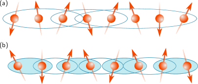
Figure 1: Illustration of local entanglement structure in ETH (a) and many-body localized phase (b) of a random spin chain. In the ETH phase the entanglement is shared among all spins, which give rise to volume law bipartite entanglement. In contrast many-body localized phase has an area law entanglement and a large part of entanglement is stored in nearest neighbor spins.

These excited states are characterized by large entanglement between subsystems. In fact, the entanglement is typically nearly the maximum possible bipartite entanglement, that goes as $\log N$ where $N$ is the dimensionality of the Hilbert space of the smaller subsystem.

This is then proportional to the number of particles in the subsystem and this extensive situation is referred as the volume law Grover ; Kjäll et al. (2014); Luitz et al. (2015). In this regime the eigenstates have large multipartite entanglement and we can expect that the entanglement among small subsystems is absent (see Fig. 1 for an illustration). Exactly how large the subsystems must be before they become entangled has been explored in the case of random states Bhosale et al. (2012).

In the extreme case, the entanglement between two spins in a spin chain whose state obeys the volume law is typically zero. However if there is a transition to a localized phase where the ETH is violated, it can also be characterized by the appearance of entanglement among such small subsystems as described in Fig. 1. Thus the purpose of this paper is to study the well-established measure of concurrence to measure the entanglement between two spin$-1/2$ particles when the whole system undergoes a transition to a MBL phase. Although several remarks about entanglement in the MBL phase were inferred from spin-correlations in the past, for example in Ref. Pal and Huse, 2010, we are not aware of works that calculate the actual entanglement between two spins across the many-body localization transition.

Moreover, concurrence is an entanglement monotone that has been measured experimentally in some contexts. In trapped atomic ion Jurcevic et al. (2014) and cold atom Fukuhara et al. (2015) setup the concurrence dynamics after a global quench has been measured. Therefore understanding the behaviour of concurrence across the many-body localization transition will be useful for future experiments.

II Model and method

Consider a model in which the transition to a MBL phase has been well-studied already Pal and Huse (2010), the XXZ spin-chain:

$$H=\dfrac{1}{2}\left(\sum_{i=1}^{L-1}\sigma^{x}_{i}\sigma^{x}_{i+1}+\sigma^{y}_{i}\sigma^{y}_{i+1}+\Delta\sigma^{z}_{i}\sigma^{z}_{i+1}\right)+\sum_{i=1}^{L}h_{i}\sigma^{z}_{i},$$ (1)

where $h_{i}$ is a random magnetic field chosen from the uniform distribution on the interval $[-W,W]$ and $\Delta$ is an interaction strength. If $\Delta=0$ the model is equivalent to one of non-interacting fermions and even with the disordered magnetic field, it is integrable. The fluctuations of the energy levels is that of independent random variables and for example the unfolded nearest neighbor spacing distribution is Poisson ($e^{-s}$, where $s$ is the normalized nearest energy level spacing). When $\Delta$ is tuned away from zero, there is interaction in the underlying fermion model, and the nearest neighbor spacing for example could become that of the Gaussian Orthogonal Ensemble (GOE), that is of relevance to time-reversal symmetric complex quantum systems, and is characterized by level repulsion and spectral rigidity. The eigenstates in this phase have a volume law, and possess large multipartite entanglement.

However for a given interaction, if the disorder strength is sufficiently large, there is a transition from this ETH phase to the MBL phase and the Poisson level statistics reappears. This signals an interacting but localized phase, and is one of the first ways in which the MBL transition was studied. For the Hamiltonian defined in Eq. (1) when $\Delta=1$, such a transition is believed to happen when $W$ exceeds $\approx 3.5$ in the large system size $L$ limit Pal and Huse (2010); Berkelbach and Reichman (2010); De Luca and Scardicchio (2013); Bar Lev et al. (2015); Luitz et al. (2015); Bera et al. (2015).

We will study the above mentioned model (Eq. (1)) using the exact diagonalization method at finite system sizes $L=10,12,14,16$ and $18$ with open boundary condition. Typically for small system sizes upto $10^{4}$ disorder realizations are used to perform the disorder average and $500$ disorder realizations for $L=18$. Around 50 states are used from the middle of the spectrum to perform an additional average to decrease the statistical noise.

The MBL transition has been characterized in ways other than a transition in level statistics, mainly through various properties of the eigenstates. Entanglement has also been extensively studied in these transitions Kjäll et al. (2014); Grover ; Luitz et al. (2015) and fluctuation of the von Neumann entropy between two halves of the spin chain shows a maximum around the transition point. In all of these studies states are considered that are well away from either ends of the spectra: the ground state or the most excited state. It may be noted that a logarithmic growth of entanglement entropy in non-stationary states is also seen as a sign of interactions in such spin systems Žnidarič et al. (2008); Bardarson et al. (2012); Serbyn et al. (2013).

While such previous studies concentrate on the entanglement between two halves of the system, that may be characterized as macroscopic entanglement, this paper considers the complementary question of inter-spin entanglement. It is well-known that while the entanglement between any bipartition of a many-body system in a collective pure state can be measured as the von-Neumann entropy of any of the two subsystems, there is no such measure when the collective state is mixed. However the entanglement in the mixed state of two spin-1/2 particles is an exception, and concurrence Hill and Wootters (1997); Wootters (1998) has long been used as such a measure. The entanglement of formation is a monotonic function of concurrence, and it arises as a solution of a optimization problem. It has been used in numerous studies of spin chains and in particular derivatives of it can be an order parameter in low-temperature quantum phase transitions, such as in the XY and transverse Ising model Osterloh et al. (2002).

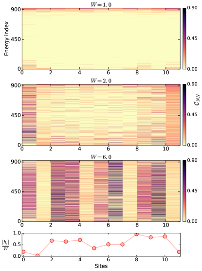
Figure 2: The nearest-neighbor concurrence $\mathcal{C}_{NN}$ in eigenstates of the XXZ model is shown as the intensity for a given disorder configuration. The vertical axis is the state number, with the ground state being $0$. The horizontal axis has the $11$ nearest pairs with $L=12$ spins and $\Delta=1$. The disorder strength $W=1.0$, $W=2.0$ and $W=6.0$ from top in the first three panels. The disorder configuration ($h_{i}$ when $W=1$) is identical in all cases and is shown in the last panel. This highlights that in the MBL phase the concurrence is correlated with disorder configuration and probe the resonances in the configuration.

II.1 Concurrence as a measure of two body entanglement

For completeness, concurrence is first defined in Ref. Wootters, 1998, for further details see also Ref. Amico et al., 2008. If $L$ spins are in a joint pure state $|\psi\rangle$, let $\rho_{ij}$ be the state of two spins, one at site $i$ and the other at $j$. It is in general a mixed state and the von Neumann entropy of the single spin reduced density matrices (RDM) does not have the interpretation of being the entanglement between the two spins. The state $\rho_{ij}$ is separable if there exists single spin density matrices $\rho_{i}^{k}$ and $\rho_{j}^{k}$ such that $\rho_{ij}=\sum_{k}p_{k}\,\rho_{i}^{k}\otimes\rho_{j}^{k}$, where $p_{k}$ are probabilities. If this is not possible, the mixed state is entangled. Thus for mixed states entanglement is a more subtle property than not being a product state. One of the central reasons for the difference is that mixed states can arise as mixtures of pure states in infinitely many physically different ways Nielsen and Chuang (2000).

The set of two-spin states $\{|\phi_{k}\rangle\}$ is a purification of $\rho_{ij}$ if $\rho_{ij}=\sum_{k}p_{k}|\phi_{k}\rangle\langle\phi_{k}|$, where $\{p_{k}\}$ are such that they are non-negative and add to $1$ (i.e. are probabilities). The entanglement of formation is defined as the minimum value of the average entanglement $\sum_{k}p_{k}{\cal E}(|\phi_{k}\rangle)$, where ${\cal E}(|\phi_{k}\rangle)$ is the entanglement of the pure bipartite state. The minimization is over all the (infinite) possible purifications. While this problem is hard in general, for two spin $1/2$ particles it was solved when it was shown that the concurrence as defined below is a monotonic function of the entanglement of formation.

The concurrence in two qubits $i$ and $j$ that are in the joint state $\rho_{ij}$ is given by the following procedure Wootters (1998): Construct the matrix $\rho_{ij}\,\tilde{\rho}_{ij}$, where $\tilde{\rho}_{ij}=\,\sigma^{y}\otimes\sigma^{y}\rho_{ij}^{*}\sigma^{y}\otimes\sigma^{y}$, and the complex conjugation is done in the standard computational basis. Let the eigenvalues (guaranteed to be positive) be $\{\lambda_{1}\geq\lambda_{2}\geq\lambda_{3}\geq\lambda_{4}\}$, then the concurrence is $\mathcal{C}_{i,j}=\mbox{max}\left(\sqrt{\lambda_{1}}-\sqrt{\lambda_{2}}-\sqrt{\lambda_{3}}-\sqrt{\lambda_{4}},\,0\right)$. This is such that $0\leq\mathcal{C}_{i,j}\leq 1$, with the concurrence vanishing only for separable states and reaches unity for maximally entangled ones such as the singlet state.

The Hamiltonian in Eq. (1) commutes with the total spin $\sum_{i}\sigma_{i}^{z}$. Attention in this paper is restricted to the total spin $0$ sector. The conservation of total spin is a strong condition and in this case the non-zero elements of the two-spin reduced density matrix $\rho_{ij}$ can be written in terms of spin-expectation values as

$$\begin{split}&\langle ab|\rho_{ij}|ab\rangle=\dfrac{1}{4}\langle(1-(-1)^{a}\sigma_{i}^{z})(1-(-1)^{b}\sigma_{j}^{z})\rangle,\;a,b\in\{0,1\},\\ &\langle 01|\rho_{ij}|10\rangle=\langle\sigma^{+}_{i}\sigma^{-}_{j}\rangle,\,\langle 10|\rho_{ij}|01\rangle=\langle\sigma^{-}_{i}\sigma^{+}_{j}\rangle.\end{split}$$ (2)

Here $\{|0\rangle,\,|1\rangle\}$ are eigenstates of $\sigma^{z}$ with eigenvalues $\pm 1$ respectively and $\sigma^{\pm}=\frac{1}{2}(\sigma^{x}\pm i\sigma^{y})$, or $\sigma^{+}=|0\rangle\langle 1|$, $\sigma^{-}=|1\rangle\langle 0|$. There are only $3$ real independent diagonal elements and one complex off-diagonal element in $\rho_{ij}$. The block-diagonal structure of such density matrices makes the concurrence in the state turn out to be of a simpler form O’Connor and Wootters (2001):

$$\mathcal{C}_{i,j}=2\,\mbox{max}\{|z|-\sqrt{xy},\,0\},$$ (3)

where $z=\langle 01|\rho_{ij}|10\rangle$, $x=\langle 00|\rho_{ij}|00\rangle$ and $y=\langle 11|\rho_{ij}|11\rangle$.

For definiteness we refer to states now as being composed of qubits or two-state particles, with the eigenstates labeled by $0$ and $1$ in the computational basis. The isomorphism with spin-1/2 states is evident. Monogamy of entanglement refers to the property that when two qubits are maximally entangled, then they cannot be entangled with any other qubits. This uniquely quantum correlation also means that entanglement is shared in a many-body situation in many ways. It is known that in typical or random states of many qubits, multipartite entanglement is shared among many qubits rather than in a pairwise manner. For such states the probability that any two qubits are entangled is vanishingly small if the total number exceeds about $6$ Scott and Caves (2003). In states that have further restrictions, for example restricted to a definite number of $0$ states, there could be enhanced concurrences. In one-particle states that correspond to superpositions of one qubit in the $0$ state, with the rest in $1$ (or vice-versa), typical pairs of qubits can have fairly large entanglement with the concurrence decreasing as $1/L$ Lakshminarayan and Subrahmanyam (2003), where $L$ is the total number of qubits. For two-particle states it decreases as $1/L^{2}$, but for three and higher particle states it is exponentially small Vijayaraghavan et al. (2011) in $L$. Thus finding two qubit entanglement in a complex state, is rare.

III Results and Discussions

In this section, we first describe the behavior of nearest neighbor concurrence in the many-body energy spectrum for a typical disorder realization. Next the scaling of average nearest neighbor concurrence is studied across the many-body localization transition. Finally we discuss the dependence of the concurrence on neighboring spin distances and system sizes in the localized phase.

III.1 Nearest neighbor concurrence across the many-body energy spectrum and resonances in disorder configuration

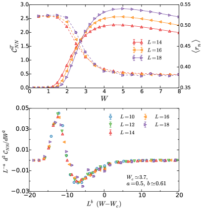
Figure 3: Upper panel shows the the total nearest neighbor concurrence (solid lines) and average of nearest energy level spacing ratios (dotted lines) $\langle r_{n}\rangle$ for three different system sizes as a function of disorder strength for $\Delta=1.0$. It is clear that the many-body localization transition is captured similarly as in nearest energy level spacing and in concurrence. Lower panel shows a scaling collapse of the second derivative of the average nearest neighbor concurrence with respect to disorder. From the scaling collapse critical disorder is estimated to be $W_{c}=3.7\pm 0.2$.

Typical concurrence

In Fig. 2 the nearest-neighbor concurrence is shown as a function of the energy across an entire spectrum for a specific disorder configuration and three different strengths. Top panel shows the concurrence for small disorder, while the middle panel for disorder values near the transition point $W=2$ and the lower panel for disorder value $W=6$, which is in the localized phase for system size $L=12$. The lowest panel shows the particular disorder configuration that is used in the calculation. For small disorder strength, but sufficiently far from the integrable value of $W=0$ the ETH or random phase dominates the spectra, except at the spectrum edges. It is clearly seen that in this case concurrence is present dominantly only in the lowest or highest excitations. The bulk of the states are free from nearest neighbor entanglement and in fact of any kind of two-body entanglement, suggesting that the other spins are acting as a thermal reservoir, and consistent with the fact that random matrix theory (RMT) fluctuations, particularly that of the Gaussian Orthogonal Ensemble (GOE) is obtained here. This also confirms that the ground state (and the lowest excited states) is in the localized phase and the many-body localization transition is an excited state phase transition.

Additionally it is also interesting to observe that the low lying excitations and the ground state have very large nearest neighbor entanglement. For translationally invariant states, under certain constraints, it was shown that the maximum possible nearest neighbor concurrence is about 0.434, and values close to this are indeed observed for the Heisenberg model O’Connor and Wootters (2001), which corresponds here to $W=0$ and $\Delta=1$. It is therefore quite surprising to find such persistently large entanglement in the non-integrable case of $W=1$ when the bulk of the spectral fluctuations are that of RMT. The emphasis in this paper though will be on the excited states at the center of the spectrum or in the infinite temperature limit.

Resonances in disorder configuration

For higher values of disorder strength, it is clear from Fig. 2 that there is as strong variability in the concurrence across a spin chain for a given disorder configuration. In particular, it is interesting to note that in the localized phase across the energy spectrum large value of concurrence forms bands that is related to the disorder configuration. The configuration is also shown at the bottom of the figure and it is quite clear that there is a correspondence: if $|h_{i+1}-h_{i}|$ is small ($\ll 1$) there is larger concurrence between spins $i$ and $i+1$. A heuristic understanding of this follows from the observation that for large $W$ the energy due to the external field may be considered the dominant one and the rest a perturbation. Concentrating on two neighboring spins $i$ and $i+1$, their unperturbed energies are $h_{i}+h_{i+1}$, $-h_{i}+h_{i+1}$, $h_{i}-h_{i+1}$ and $-h_{i}-h_{i+1}$, corresponding to the spin configurations $00$, $10$, $01$ and $11$. When $h_{i}\approx h_{i+1}$ the perturbations can strongly couple $01$ and $10$ to create entanglement (and concurrence) between the spins. In the opposite case when $h_{i}\approx-h_{i+1}$ it may seem that the configurations $00$ and $11$ may also couple to create entanglement, however as the perturbations preserve total spin, there is no matrix elements to create this, and hence the dominant concurrences occur essentially due to resonances in the disorder configuration.

Perturbative analysis

To be more concrete consider the extreme case of $L=2$. This is also relevant for larger $L$ when the configuration consists primarily of the first $L/2$ spins in say $0$ and the other in $1$. The perturbation that mixes into this state when $W<\infty$ flips only the central two spins which then get entangled. For a state of the form $\alpha|01\rangle+\beta|10\rangle$ the concurrence is $2|\alpha\beta|$. A simple calculation then gives that

$$\mathcal{C}_{NN}=\frac{1}{\sqrt{1+(h_{1}-h_{2})^{2}}},$$ (4)

which shows that when $h_{1}=h_{2}$ the concurrence is the maximum possible and $NN$ stands for nearest-neighbor. Considering that $h_{i}$ are sampled uniformly in $[-W,W]$, the average concurrence is

$$\begin{split}\langle\mathcal{C}_{NN}\rangle&=\frac{1}{2W^{2}}\,\left(2W\,\sinh^{-1}(2W)+1-\sqrt{1+4W^{2}}\right)\\ &=\frac{1}{W}(\ln W+\ln 4-1)+\mathcal{O}(1/W^{2}),\end{split}$$ (5)

showing how the concurrence vanishes when the disorder strength is increased to infinity. Numerical results are presented below for larger number of spins, but it is noteworthy that the $L=2$ averages reflect the rather large concurrence present in the MBL phase. For instance the average value of concurrence from the above formula is $0.32$ for $W=8$. As the number of spins increase this decreases as well, and the interplay of concurrence as a function of $L$ and $W$ is investigated as a scaling relation.

III.2 Average concurrence, finite size scaling and qualitative phase diagram

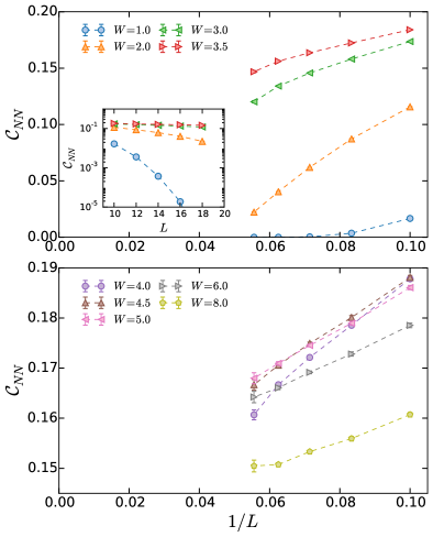
Figure 4: The nearest neighbor concurrence averaged over pairs and disorder configurations is shown as a function of (inverse) system sizes for various values of the disorder strengths, while the interaction $\Delta=1$. The concurrence for a fixed disorder strength seems to survive in the thermodynamic limit in the MBL phase (lower panel), while it vanishes exponentially or faster in the ETH phase (upper panel) as suggested by the inset of the top panel where the scale is linear-log.

Average nearest-neighbor concurrence

In this section we will mainly concentrate on the average concurrence at finite energy densities. In particular, we concentrate at the middle of the energy spectrum, which corresponds to the infinite temperature limit in the thermodynamic system. Finally the energy dependence of the total concurrence will also be discussed. Top panel of Fig. 3 shows the total nearest neighbor concurrence,

$$C^{T}_{NN}=\sum_{i=1}^{L-1}\mathcal{C}_{i,i+1},$$ (6)

averaged over disorder configurations for three cases of $L=10,12$ and $14$. Shown in the same figure for convenience and comparison is the energy level average nearest neighbor spacing ratio, $\langle r_{n}\rangle$. This spacing ratio is well-known to undergo a transition (after the initial integrable to GOE transition at $W=0$) from GOE to Poisson as the disorder strength $W$ increases. The Poisson value of $\langle r_{n}\rangle$ is $\approx 0.39$ while that of the GOE is $\approx 0.53$ Atas et al. (2013).

Figure 5: The nearest neighbor concurrence averaged over sites and disorder configurations is shown as a function of a normalized excitation level ($n/N$, where $n$ is the state’s number and $N$ the number of states) and disorder strength. $L=12$ spins have been taken and averaged over $3\times 10^{3}$ disorder realizations. Special nature of the low lying excitations are also visible as large concurrence.

It is clear from Fig. 3 that when the nearest neighbor energy spacing distribution is that of the GOE concurrence is practically non-existent between any pair of neighboring spins. In fact no pair of spins are entangled. As soon as $\langle r_{n}\rangle$ starts to deviate from the GOE value, it also heralds the creation of two-spin entanglements as measured by the concurrence. Shown is simply the total of such entanglements between neighboring pairs of spins. It is seen that just after the RMT phase the total concurrence decreases with increasing system size, and we may expect that in the thermodynamic limit it even vanishes. However it is seen that the total concurrence curves cross each other at a value of $W$ that is roughly constant and occurs around the value where a transition to MBL is suggested to happen. Beyond this critical value of $W$, larger system sizes imply larger total concurrence. As will be presently shown most of the concurrence, when present, is in the nearest neighbors. It may be remarked that the average nearest neighbor concurrence per pair of spins $\mathcal{C}_{NN}^{T}/(L-1)$ decreases uniformly with $L$, across the entire range of $W$. At large disorder, though, the effect of finite size systems becomes more evident. In a sense that within these system sizes we observe that the concurrence decays as $1/W$, which is a result of a simple perturbation theory for large $W$. The very fact that the perturbation theory works suggest that the effect of interaction in this regime for this particular observable is negligible and the dominant physics is due to conventional Anderson localization rather the MBL, which is primarily due to interplay of interaction and disorder.

Finite size scaling

In order to quantify the critical point of the phase transition, we look at the derivatives of the concurrence as a function of disorder. The lower panel of Fig. 3 shows a scaling collapse of second derivative of the concurrence for different values of systems sizes. We choose the following scaling form to perform the finite size scaling analysis

$$\frac{d^{2}\mathcal{C}^{T}_{NN}}{dW^{2}}=L^{a}\Phi(L^{b}(W-W_{c})),$$ (7)

where $\Phi$ is an unknown scaling function, which in practice is determined by the chi-square minimization procedure. In the lower panel of Fig. 3 the collapse is observed for the following parameters: $W_{c}=3.7\pm 0.2$, $a\simeq 0.5$ and $b=0.6\pm 0.1$. The scatter in the $L=18$ data set is due to numerical noise and large statistical fluctuation. Such a uniform scaling collapse before and after the transition could be obtained for the second derivative, but not the concurrence or its first derivative. The critical value obtained is in agreement with those obtained by other measures Pal and Huse (2010); Luitz et al. (2015); Bera et al. (2015), although recently a larger critical disorder value in this model has also been predicted Devakul and Singh (2015).

L-dependence

Fig. 4 shows the average concurrence per pair of nearest neighbor spins as a function of system size $L$. As mentioned in the introduction random states are expected to have concurrence that is at least super-exponentially small in $L$. This is consistent with the data in the top panel of this figure for $W=1$, where except for small system sizes the probability of finding non-zero concurrence is negligible. For higher values of $W$, such as $3$, an exponential dependence seems plausible. In the transition region and in the deep MBL phase the behavior with systems size is very different showing a tendency for there to be entanglement in the large system size limit. This in turn reflects the quasi-integrable nature of the states in this phase.

Qualitative phase diagram

Fig. 5 shows the average (over sites and disorder configurations) nearest neighbor concurrence, as a function of energy density and disorder strength. A typical picture emerges showing that for a given disorder strength ETH behavior sets in at excited states. The qualitative pictures is consistent with earlier studies in a sense that at small energy density the states are localized thus the concurrence is finite. Whereas in the ETH phase the concurrence is strictly zero. In the middle of the spectrum the phase transition happens $W_{c}\ll 3.7$ for system size $L=12$. The special nature of the low-lying excitations are visible as those with large concurrence.

III.3 Finite range of entanglement in the many-body localized phase

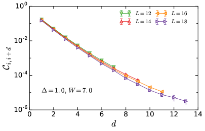
Figure 6: The concurrence averaged over sites and disorder configurations is shown as a function of distance for different systems sizes ($L=12,\ldots,18$) in the MBL phase. The y-axis is in log scale to emphasize the exponential decay of average concurrence in the localized phase. The parameters are $W=7.0$ and $\Delta=1.0$. Note that in the ETH phase the concurrence is strictly zero across the chain length.

Exponential decay of entanglement

To understand the range of entanglement in the localized phase we investigate the concurrence in a given system size $L$. Fig. 6 shows the entanglement between pairs of spins as a function of distance between them in a linear-log plot for disorder $W=7.0$ and interaction $\Delta=1.0$. The average of $\mathcal{C}_{i,i+d}$ is calculated for a given $d$ over different disorder realizations and sites $i$ and numerical data supports

$$\mathcal{C}_{i,i+d}\sim\mathcal{C}_{i,i+1}\exp(-d/\xi_{E}),$$ (8)

that is at short distances $d\ll L$ the decay of concurrence is exponential. With increasing distance the concurrence as a function of distance has a slight curvature, which is related to finite size effects. It is interesting to note that the exponential decay of concurrence in the localized phase is reminiscent of exponential decay of correlation. However, in the ergodic phase the behaviour is completely reversed in a sense that spins are long range correlated but any two body entanglement (even nearest neighbor) is absent. As mentioned above inferences about entanglement from correlation could be misleading.

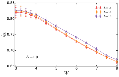
Figure 7: The entanglement length scale $\xi_{E}$ as function of the disorder for different systems sizes ($L=14,16,18$). The entanglement length is extracted by fitting the concurrence with Eq. (8). The saturation of the entanglement length close to the transition could be related to finite size effects.

Entanglement length

Fig. (7) shows the variation of the entanglement length $\xi_{E}$ with the disorder strength $W$ for various system sizes. It is interesting that in the range of parameters where the MBL transition happens (around $3-4$) there are substantial fluctuations in the entanglement length which is also large. As the MBL phase sets in the fluctuations are smaller and a more or less linear decrease in the localization length is observed.

IV Conclusions

In this work we proposed a way to investigate the local entanglement structure across the many-body localization transition by measuring the concurrence. First, we showed that the nearest neighbor concurrence, which is a measure of entanglement between two spins is intimately related to the disorder configuration. In particular, larger concurrence between two nearest neighbor spins corresponds to smaller difference between neighboring disorder configuration. This is clearly visible in Fig. 2 and consistent across the many body energy spectrum in the localized phase.

We further investigated the average concurrence at finite energy density and showed that in the RMT phase the concurrence vanishes exactly, implying all spins pair are disentangled. The entanglement is shared between all spins, which give rise to volume law bipartite entanglement entropy behaviour in an eigenstate. In the MBL phase the concurrence is finite and the total nearest neighbor concurrence increases with increasing system sizes. At even stronger disorder ($W\gtrsim 6.5$ for $\Delta=1$ and $L=18$) the concurrence decreases as $1/W$. The decrease can be understood from the perturbative analysis in the large disorder limit. The fact that in this limit the perturbative analysis is valid is an interesting observation. The validity of the perturbation theory strongly suggests that in this regime the effect of interaction is small and the physics is dominated by conventional Anderson localization rather than the many-body localization effect for these small system sizes for this observable. Eventually, in the thermodynamic limit, $L\rightarrow\infty$, one would expect that the decay of concurrence will be delayed and will be pushed to infinite disorder strength, such that the MBL phase will have a finite concurrence.

The above fact is confirmed by analysing the system size dependence of the average nearest neighbor concurrence, $\mathcal{C}_{NN}$. It is found that in the RMT phase the concurrence decay super-exponentially with the system size, whereas in the MBL phase the $\mathcal{C}_{NN}$ is showing a tendency to survive in the thermodynamic limit.

Next, to accurately calculate the phase transition we looked at the non-analyticity of the second derivative of the concurrence with respect to disorder, which is related to the variance. By performing a finite size scaling analysis we found the critical disorder strength to be around $W_{c}=3.7\pm 0.2$, which is consistent with previously estimated value using other observables, including nearest energy level spacing.

Finally, we studied the distant spins concurrence in the MBL phase. We found that at small distance between spins the concurrence decay exponentially with the distance. The correlation length associated with the decay is also investigated and found to be saturating close to the transition point.

Several interesting directions of further research are opened due to the understanding of the concurrence in MBL phase. In particular, the dynamics of the concurrence after a quench is an immediate extension of this work. Furthermore, it would be fruitful to understand how much quantum entanglement is stored in local spins during unitary evolution in the localized phase, which could be used for storing quantum memory in future applications. Very recently the propagation of concurrence has been measured in a trapped atomic ion setup Jurcevic et al. (2014) and in a Bose-Hubbard chain in an optical lattice Fukuhara et al. (2015); thus studying the dynamics after a quench in the MBL phase will also be experimentally relevant.

V Acknowledgment

We are grateful to Jens H Bardarson, Frank Pollmann and Giuseppe De Tomasi for several insightful discussions and in particular, to Jens H Bardarson for collaboration on a related work. We would also like to thank MPIPKS visitor program for hospitality.

References

- Kramer and MacKinnon (1993) B. Kramer and A. MacKinnon, Rep. Prog. Phys. 56, 1469 (1993).
- Evers and Mirlin (2008) F. Evers and A. D. Mirlin, Rev. Mod. Phys. 80, 1355 (2008).
- Basko et al. (2006) D. M. Basko, I. L. Aleiner, and B. L. Altshuler, Ann. Phys. 321, 1126 (2006).
- Gornyi et al. (2005) I. V. Gornyi, A. D. Mirlin, and D. G. Polyakov, Phys. Rev. Lett. 95, 206603 (2005).
- Oganesyan and Huse (2007) V. Oganesyan and D. A. Huse, Phys. Rev. B 75, 155111 (2007).
- Nandikishore and Huse (2015) R. Nandikishore and D. Huse, Annu. Rev. Condens. Matter Phys. 6, 15 (2015).
- Altman and Vosk (2015) E. Altman and R. Vosk, Annual Review of Condensed Matter Physics 6, 383 (2015).
- Žnidarič et al. (2008) M. Žnidarič, T. Prosen, and P. Prelovšek, Phys. Rev. B 77, 064426 (2008).
- Pal and Huse (2010) A. Pal and D. A. Huse, Phys. Rev. B 82, 174411 (2010).
- Berkelbach and Reichman (2010) T. C. Berkelbach and D. R. Reichman, Phys. Rev. B 81, 224429 (2010).
- Monthus and Garel (2010) C. Monthus and T. Garel, Phys. Rev. B 81, 134202 (2010).
- Bardarson et al. (2012) J. H. Bardarson, F. Pollmann, and J. E. Moore, Phys. Rev. Lett. 109, 017202 (2012).
- Iyer et al. (2013) S. Iyer, V. Oganesyan, G. Refael, and D. A. Huse, Phys. Rev. B 87, 134202 (2013).
- Huse et al. (2013) D. A. Huse, R. Nandkishore, V. Oganesyan, A. Pal, and S. L. Sondhi, Phys. Rev. B 88, 014206 (2013).
- Serbyn et al. (2013) M. Serbyn, Z. Papić, and D. A. Abanin, Phys. Rev. Lett. 110, 260601 (2013).
- Bauer and Nayak (2013) B. Bauer and C. Nayak, J. Stat. Mech. P09005 (2013).
- (17) J. Z. Imbrie, arXiv:1403.7837 .
- Vosk and Altman (2014) R. Vosk and E. Altman, Phys. Rev. Lett. 112, 217204 (2014).
- Pekker et al. (2014) D. Pekker, G. Refael, E. Altman, E. Demler, and V. Oganesyan, Phys. Rev. X 4, 011052 (2014).
- Kjäll et al. (2014) J. A. Kjäll, J. H. Bardarson, and F. Pollmann, Phys. Rev. Lett. 113, 107204 (2014).
- Laumann et al. (2014) C. R. Laumann, A. Pal, and A. Scardicchio, Phys. Rev. Lett. 113, 200405 (2014).
- Andraschko et al. (2014) F. Andraschko, T. Enss, and J. Sirker, Phys. Rev. Lett. 113, 217201 (2014).
- Chandran et al. (2014) A. Chandran, V. Khemani, C. R. Laumann, and S. L. Sondhi, Phys. Rev. B 89, 144201 (2014).
- De Luca et al. (2014) A. De Luca, B. L. Altshuler, V. E. Kravtsov, and A. Scardicchio, Phys. Rev. Lett. 113, 046806 (2014).
- Luitz et al. (2015) D. J. Luitz, N. Laflorencie, and F. Alet, Phys. Rev. B 91, 081103 (2015).
- Lazarides et al. (2015) A. Lazarides, A. Das, and R. Moessner, Phys. Rev. Lett. 115, 030402 (2015).
- Ponte et al. (2015) P. Ponte, Z. Papić, F. Huveneers, and D. A. Abanin, Phys. Rev. Lett. 114, 140401 (2015).
- Agarwal et al. (2015) K. Agarwal, S. Gopalakrishnan, M. Knap, M. Müller, and E. Demler, Phys. Rev. Lett. 114, 160401 (2015).
- Bera et al. (2015) S. Bera, H. Schomerus, F. Heidrich-Meisner, and J. H. Bardarson, Phys. Rev. Lett. 115, 046603 (2015).
- Johri et al. (2015) S. Johri, R. Nandkishore, and R. N. Bhatt, Phys. Rev. Lett. 114, 117401 (2015).
- Devakul and Singh (2015) T. Devakul and R. R. P. Singh, Phys. Rev. Lett. 115, 187201 (2015).
- Li et al. (2015) X. Li, S. Ganeshan, J. H. Pixley, and S. Das Sarma, Phys. Rev. Lett. 115, 186601 (2015).
- Modak and Mukerjee (2015) R. Modak and S. Mukerjee, Phys. Rev. Lett. 115, 230401 (2015).
- Schreiber et al. (2015) M. Schreiber, S. S. Hodgman, P. Bordia, H. P. Lüschen, M. H. Fischer, R. Vosk, E. Altman, U. Schneider, and I. Bloch, Science 349, 842 (2015).
- Bordia et al. (2015) P. Bordia, H. P. Lüschen, S. S. Hodgman, M. Schreiber, I. Bloch, and U. Schneider, arXiv:1509.00478 (2015).
- Ovadia et al. (2015) M. Ovadia, D. Kalok, I. Tamir, S. Mitra, B. Sacépé, and D. Shahar, Scientific Reports 5, 13503 EP (2015).
- Smith et al. (2015) J. Smith, A. Lee, P. Richerme, B. Neyenhuis, P. W. Hess, P. Hauke, M. Heyl, D. A. Huse, and C. Monroe, arXiv:1508.07026 (2015).
- Deutsch (1991) J. M. Deutsch, Phys. Rev. A 43, 2046 (1991).
- Srednicki (1994) M. Srednicki, Phys. Rev. E 50, 888 (1994).
- Srednicki (1999) M. Srednicki, Journal of Physics A: Mathematical and General 32, 1163 (1999).
- Rigol et al. (2008) M. Rigol, V. Dunjko, and M. Olshanii, Nature 452, 854 (2008).
- Mehta (2004) M. L. Mehta, Random Matrices (Elsevier Academic Press, 3rd Edition, London, 2004).
- Giannoni et al. (1991) M. J. Giannoni, A. Voros, and J. Zinn-Justin, eds., Chaos and Quantum Physics (North-Holland, Amsterdam, 1991) pp. 547–663.
- Karthik et al. (2007) J. Karthik, A. Sharma, and A. Lakshminarayan, Phys. Rev. A 75, 022304 (2007).
- Kim and Huse (2013) H. Kim and D. A. Huse, Phys. Rev. Lett. 111, 127205 (2013).
- Kollath et al. (2007) C. Kollath, A. M. Läuchli, and E. Altman, Phys. Rev. Lett. 98, 180601 (2007).
- Trotzky et al. (2012) S. Trotzky, Y.-A. Chen, A. Flesch, I. P. McCulloch, U. Schollwock, J. Eisert, and I. Bloch, Nat Phys 8, 325 (2012).
- Sorg et al. (2014) S. Sorg, L. Vidmar, L. Pollet, and F. Heidrich-Meisner, Phys. Rev. A 90, 033606 (2014).
- Schlagheck and Shepelyansky (2015) P. Schlagheck and D. L. Shepelyansky, arXiv:1510.01864 (2015).
- (50) T. Grover, arXiv:1405.1471 .
- Bhosale et al. (2012) U. T. Bhosale, S. Tomsovic, and A. Lakshminarayan, Phys. Rev. A 85, 062331 (2012).
- Jurcevic et al. (2014) P. Jurcevic, B. P. Lanyon, P. Hauke, C. Hempel, P. Zoller, R. Blatt, and C. F. Roos, Nature 511, 202 (2014).
- Fukuhara et al. (2015) T. Fukuhara, S. Hild, J. Zeiher, P. Schauß, I. Bloch, M. Endres, and C. Gross, Phys. Rev. Lett. 115, 035302 (2015).
- De Luca and Scardicchio (2013) A. De Luca and A. Scardicchio, EPL 101, 37003 (2013).
- Bar Lev et al. (2015) Y. Bar Lev, G. Cohen, and D. R. Reichman, Phys. Rev. Lett. 114, 100601 (2015).
- Hill and Wootters (1997) S. Hill and W. K. Wootters, Phys. Rev. Lett. 78, 5022 (1997).
- Wootters (1998) W. K. Wootters, Phys. Rev. Lett. 80, 10 (1998).
- Osterloh et al. (2002) A. Osterloh, L. Amico, G. Falci, and R. Fazio, Nature 416, 608 (2002).
- Amico et al. (2008) L. Amico, R. Fazio, A. Osterloh, and V. Vedral, Rev. Mod. Phys. 80, 517 (2008).
- Nielsen and Chuang (2000) M. A. Nielsen and I. L. Chuang, Quantum Computation and Quantum Information (Cambridge University Press, Cambridge, 2000).
- O’Connor and Wootters (2001) K. M. O’Connor and W. K. Wootters, Phys. Rev. A 63, 052302 (2001).
- Scott and Caves (2003) A. J. Scott and C. M. Caves, Journal of Physics A: Mathematical and General 36, 9553 (2003).
- Lakshminarayan and Subrahmanyam (2003) A. Lakshminarayan and V. Subrahmanyam, Phys. Rev. A 67, 052304 (2003).
- Vijayaraghavan et al. (2011) V. S. Vijayaraghavan, U. T. Bhosale, and A. Lakshminarayan, Phys. Rev. A 84, 032306 (2011).
- Atas et al. (2013) Y. Y. Atas, E. Bogomolny, O. Giraud, and G. Roux, Phys. Rev. Lett. 110, 084101 (2013).