An individual-based model for biofilm formation at liquid surfaces

Abstract

The bacterium Bacilus subtilis frequently forms biofilms at the interface between the culture medium and the air. We develop a mathematical model that couples a description of bacteria as individual discrete objects to the standard advection-diffusion equations for the environment. The model takes into account two different bacterial phenotypes. In the motile state, bacteria swim and perform a run-and-tumble motion that is biased toward regions of high oxygen concentration (aerotaxis). In the matrix-producer state they excrete extracellular polymers, which allows them to connect to other bacteria and to form a biofilm. Bacteria are also advected by the fluid, and can trigger bioconvection. Numerical simulations of the model reproduce all the stages of biofilm formation observed in laboratory experiments. Finally, we study the influence of various model parameters on the dynamics and morphology of biofilms.

1 Introduction

Bacteria are unicellular prokaryotic microorganisms. They are ubiquitous and constitute a large part of the terrestrial biomass. Bacteria can live as individual cells during the planktonic phase. However, most of the time, they are part of self-organized communities of complex architecture adsorbed on interfaces: the biofilms. Besides the bacteria themselves, biofilms are mostly made of an extracellular matrix composed of macromolecules [1, 2, 3] that are produced by the bacteria and lead to cohesive interactions between them [4, 5]. Most of the time biofilms appear in aqueous environments either on solid surfaces or at the water-air interfaces. Due to this multicellular organization, the bacteria have different properties than in the motile state. For example, bacteria trapped in biofilms can exhibit an increased resistance to antibiotics as well as to environmental stresses (desiccation, UV radiation, disinfecting agents, shear flow…) [6, 7]. Therefore, the association in biofilms is a crucial step both for survival and spreading of bacterial colonies [8].

Many environmental and genetic factors influence the development of biofilms [8]. Although biofilm formation is not understood in all details, a consistent picture of biofilm growth on solid substrates has been proposed: bacteria in the planktonic phase anchor preferentially on a stable surface, which initiates the nucleation of bacterial microcolonies [5, 8]. Bacteria constituting the microcolonies secrete an extracellular matrix in which they embed, and form a mature biofilm with a complex multiscale architecture [9, 10]. Later on, bacteria can also detach from the superficial layers, return to the planktonic state and spread to new parts of the surface[11].

Much less is known on biofilm formation at water-air interfaces. We have performed laboratory experiments on Bacillus subtilis (B. subtilis) and built a mathematical model that can reproduce the main experimental observations. The details of the experimental results will be published elsewhere; here, we briefly present a summary to motivate the construction of the mathematical model.

Bacillus subtilis is a stricly aerobic bacterium which is able to form floating pellicles that can reach a thickness of several hundred microns [12] on the top of nutritive media. During a typical experiment, the nutritive medium (Luria broth supplemented with glycerol and $\textrm{MnO}_{2}$) is initially inoculated with a small concentration of bacteria. Then, the cells divide and grow over several hours to yield a homogeneous suspension (see Fig. 1 (a)). Later (Fig. 1 (b)), bacteria start to accumulate close to the interface, and a rapid transition occurs (between (b) and (c)), which leads to the nucleation of bacterial clusters on the interface (Fig. 1 (c)). At this stage, some macroscopic filaments, which can be seen inside the liquid, are advected by fluid motion. With time, the biofilm further develops into a mature floating pellicle that exhibits a typical wrinkled morphology (Fig. 1(d)).

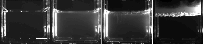
Figure 1: Side view of B. subtilis pellicle developing on top of a liquid culture media at T=$31^{\circ}$C at : (a) 0 hours, (b) 15 hours (c) 19 hours 30 minutes, and (d) 67 hours after incubation. Images are acquired with a black and white CCD camera. The scale bar is 1 cm long.

These experiments indicate several important phenomena that need be included in the model. First, B. subtilis is known to exhibit aerotaxis [13], that is, to migrate to areas in which the concentration of oxygen is high. In the experiments, the water-air interface acts as an oxygen source; therefore, aerotaxis is a possible explanation for the accumulation of bacteria close to the surface. Second, planktonic bacteria are slightly more dense than water. As a result, an accumulation of bacteria at the surface is unstable and should drive the development of bioconvection [14], which may hinder or help the biofilm formation. Finally, there is a well-defined change in bacterium phenotype from motile (planktonic phase) to matrix-producing (biofilm phase). This change is controlled by a genetic switch that is believed to be triggered by a quorum sensing mechanism [15, 10] (i.e. when the local density of bacteria exceeds a threshold value, the phenotype changes).

Many different modelling strategies have already been proposed and used for biofilm formation on solid substrates. It is possible to average the contribution of individual bacteria and to write a full continuum model [16, 17]. It is also possible to consider the bacteria as individual objects in cellular automata models (CA) [18] or individual-based models (IdbM) [19]. The latter model can be hybridized with a continuum model to describe the contribution of the environment. Modeling is often accompanied by numerical simulations to study the processes which structure the biofilm [20, 21, 22].

Here, we formulate a detailed model for biofilm formation at liquid-air interfaces. The main point is that the model captures the transition between a “gas” of individual swimming bacteria and the biofilm pellicle (a soft solid). Since this transition involves a change in the connectivity between bacteria, a description using a full continuum model is difficult. We have chosen a hybrid approach, in which the bacteria are described as individual particles, whereas the local environment (oxygen concentration, fluid velocity) is described by continuous fields. In order to keep the model minimal, we only consider two bacterial phenotypes: in the motile state, bacteria are self-propelled swimmers that perform a standard “run-and-tumble” motion. The bacteria interact through a local repulsive potential to describe collisions between bacteria (hydrodynamic interactions are neglected). In the matrix-producer state, the bacteria stop moving actively, and produce macro-molecules that constitute the extracellular matrix. Due to the presence of this matrix, they are able to “connect” to other bacteria. In this case, the interaction between bacteria is described by an attractive potential. The transition between the two phenotypes is triggered by a quorum-sensing mechanism.

This model has been implemented in two dimensions, using the discrete-element method [23] to calculate the evolution of the bacteria, and the finite-difference method [24] for the continuous fields, and simulations involving up to 10000 bacteria were performed. This setting is sufficient to demonstrate that all the steps of biofilm formation that are observed in the experiments can be reproduced. The influence of the model parameters on these different stages was also studied, yielding suggestions for further model improvements and experiments.

In the following, an overview of the model architecture is first given, followed by a detailed description of each ingredient (section 2). In section 3, the choice of the model parameters is discussed in detail. In Section 4, simulation results are presented, which demonstrate the ability of the model to properly describe biofilm formation. Finally, section 5 discusses the main conclusions and perspectives of this work.

2 Model description

2.1 Overview

Our goal is to construct a minimal mathematical model that reproduces the different steps of biofilm formation, from motile bacteria (individuals swimming in the liquid) all the way to the mature biofilm (bacteria linked by extracellular matrix). In order to include the phenomena of aerotaxis and bioconvection, the local oxygen concentration $c$ and the fluid velocity $\overrightarrow{u}$ are described as continuous fields which obey partial differential equations (PDE).

Bacteria are represented as discrete objects, with interactions that depend on their internal state. Each bacterium is characterized by its position, its velocity, and internal variables that reproduce its behavior (aerotaxis, phenotype, cell cycle). One of these internal variables is the bacterial phenotype. We take into account only two of them : motile and matrix producer. In the motile phenotype, the bacteria propel themselves with a constant velocity and change their direction with a frequency that is determined by the local concentration in oxygen (run-and-tumble motion). Each motile bacterium increases its body size with time and divides into two cells with a constant rate. In the matrix-producer state, propulsion is absent, and the bacterium produces extracellular matrix, which makes its volume grow with time (without division). Moreover, we assume that the transition from the motile to the matrix-producer phenotype is irreversible and triggered by a quorum sensing mechanism: bacteria tend to switch to the matrix-producer type when a certain bacterial concentration is (locally) exceeded.

The main effect that is caused by changing the phenotype is to change the interactions between bacteria. In both states, there is a repulsive interaction that prevents bacteria from overlapping. When a bacterium has started to produce matrix, which consists of “sticky” macromolecules, it can establish links with bacteria when they are in contact. These links correspond to a spring-like attractive interaction potential, and break when the distance between the two bacteria is above a threshold value.

In the following, we first describe how the discrete and continuum approaches are coupled, and then give more details about the description of the bacteria as discrete objects.

2.2 Environment

The geometry of the simulation setup is inspired by the experiments depicted in Fig. 1 (a container that is open at the top is filled with nutritious medium). We restrict our simulations to two dimensions, that is, the simulation domain is a vertical plane. In order to convert two-dimensional densities to three-dimensional ones that can be compared to values measured in experiments, we assume a thickness of the sample of 10$\mu$mX2x4cm². While the exact value is arbitrary, it approximately corresponds to the average diameter of the bacteria in the model. The top surface is assumed to remain perfectly flat, and it is in contact with air. The domain is discretized using a regular square grid of $N\times N/2$ points, where $N=L/\Delta x$ with $L$ being the horizontal system size (the height of the fluid layer is $L/2$), and $\Delta x$ the grid spacing, with grid points being located on the walls and on the fluid surface.

Being interested in the continuum fields on macroscopic length scales, we choose the grid spacing $\Delta x$ to be of the order of a millimeter. On this scale, the bacteria (of micron size) are point-like objects. Therefore, when an information about the environment of a bacterium is needed, the value of the relevant variable is calculated using a bilinear interpolation of the values at the three closest grid points. Conversely, the terms involving bacteria in the PDEs are computed by averaging the contribution of neighboring bacteria, as described below.

2.2.1 Density fields

In the continuum equations that are presented below, two source terms are calculated from the positions of the individual bacteria: the number density for the total oxygen consumption, and the mass density for the buoyancy force, as follows: the neighborhood of a grid point (called “cell” in the following) is defined as its Voronoi cell (the set of all points in space that are closer to it than to any other grid point). The number density $n$ is then defined by the number of bacteria that are contained in the cell, divided by the cell volume (which is smaller in the case of points located on the boundaries of the system). In order to obtain a number density $n$ with units of m^-3 that can be compared to experimental measurements, we set the thickness of the system to 10 $\mu$m, which is comparable to the the size of a bacterium.

The local mass density is also dependent on the bacterial state. Various values for the mass density of motile bacteria have been published in the literature [17, 14, 25]. Our experimental observations clearly indicate that the density of motile bacteria is larger than that of water (they sediment in the absence of active motion). The situation is not as clear for the matrix producers. If the mature biofilm is cut into pieces, some of them float, while others sink. This indicates that the biofilm density is, on average, very close to that of the medium. Therefore, we assume that matrix-producing bacteria have the same density as the medium, $\rho_{0}$, while motile bacterial density $\rho_{b}$ is slightly larger. The local mass density is then

$$\rho=\rho_{0}+\frac{V_{b}}{V_{{\rm cell}}}(\rho_{b}-\rho_{0}),$$ (1)

where $V_{{\rm cell}}$ denotes the volume of the grid cell, and $V_{b}$ the total volume occupied by motile bacteria in the cell.

While this definition is straightforward, the fact that density fields are dependent on the positions of the individual bacteria (which perform a random walk) implies that they fluctuate in space and time. The relative magnitude of these statistical fluctuations depends on the average number of bacteria in a cell, and thus decreases when the cell size is increased. The choice of the grid spacing is therefore dictated by a compromise between the spatial resolution (which requires small grid spacing) and the smoothing of the density field (which requires large grid spacings). Typically, in our simulations we have $N=20$ and up to 10000 bacteria, which yields around $50$ bacteria per cell for a homogeneous system. As a result, typical relative fluctuations are smaller than $0.2$, which is small enough to avoid spurious effects on the computation of the fluid motion and on the evaluation of the transition rate from motile to matrix producer phenotype.

2.2.2 Fluid flow calculation

Since the mass density of the bacteria is slightly higher than that of water, an accumulation of bacteria under the surface creates an unstable stratification that can give rise to convection. The medium is modeled as an incompressible Newtonian fluid with a mass density that depends on the bacterial concentration as it has been done previously in the work of Hillesdon et al [26, 27]. Its dynamics is described by the Navier-Stokes (NS) equation in the Boussinesq approximation, in which the variations of density are neglected except in the buoyancy force. Since our system is two-dimensional, we use a vorticity/stream function formulation which guarantees incompressibility, independently of the magnitude of the numerical error. In this approach, the velocity $\overrightarrow{u}$ of the fluid derives from the stream function $\psi$,

$$u_{x}=\frac{\partial\psi}{\partial y}\qquad u_{y}=-\frac{\partial\psi}{\partial x}\,.$$ (2)

which is solution of

$$\Delta\psi=-\omega\,,$$ (3)

where the time evolution of the vorticity $\omega$ writes

$$\frac{\partial\omega}{\partial t}+\left(\overrightarrow{u}\cdot\overrightarrow{\nabla}\right)\omega=\nu\triangle\omega-g\frac{\partial}{\partial x}\frac{\rho}{\rho_{0}}\;,$$ (4)

Here, $g$ is the standard gravity, and $\nu$ is the kinematic viscosity of the fluid. The left-hand side of Eq. (4) is the advective derivative of the vorticity. The two terms on the right-hand side correspond to the diffusion of the vorticity due to internal friction and to the buoyancy force, respectively. Note that we have omitted in Eq. (4) the force exerted by the bacteria on the fluid, which has been taken into account in other works (see for example [28]). This is justified since we are interested only in large-scale flow. While the force exerted by the flagella on the fluid during the run-and-tumble motion locally creates a strong agitation of the fluid, this does not lead to any macroscopic flow since the forces are averaged over many bacteria. The dominant body force term that triggers bioconvection thus is the buoyancy force.

At the bottom and side boundaries, the fluid velocity and the stream function are zero (no slip nor penetration). On the free surface between fluid and air, the vertical component of the velocity ($u_{y}$) and the tangential friction force $\left(\partial u_{x}/\partial y\right)$ are set to zero. This implies that the stream function is constant at every boundary, and we set its boundary value to be zero. Numerically, we have discretized Eq. (4) using standard finite-difference formulas on a staggered grid, and solved it with an explicit Euler scheme in time. The equation (3) was solved using a successive over-relaxation method (SOR) [24].

2.2.3 Oxygen concentration field

As mentioned earlier, bacteria accumulation potentially plays an important role in biofilm formation. Since this accumulation is mainly driven by aerotaxis, we need a proper description of the oxygen distribution in the fluid. The oxygen concentration field $c(x,y,t)$ is governed by four processes: diffusion, transport through the air-water interface, consumption by the bacteria and advection by the flow. Its evolution equation is

$$\frac{\partial c}{\partial t}+\overrightarrow{u}\cdot\overrightarrow{\nabla}c=D_{O2}\Delta c-\gamma n\frac{c}{c+K}\;.$$ (5)

Here, $\overrightarrow{u}\cdot\overrightarrow{\nabla}c$ describes the advection of the oxygen by the fluid, and $D_{O2}$ is the diffusion coefficient of oxygen in water. The consumption of oxygen by the bacteria at a concentration $n$ is modeled by a Michaelis-Menten law, which is one of the basic models for enzymatic reactions. Oxygen is consumed at a constant rate $\gamma$ by each bacterium for concentrations much larger than the Michaelis constant $K$. There are two boundary conditions for the oxygen, no flux at the walls (Neumann) and a constant concentration on the free surface (Dirichlet): on the top surface, the oxygen concentration is set to $C_{0}$ which is the saturation concentration of oxygen in water for standard conditions. Equation (5) is discretized on the same grid as the fluid flow equations, and integrated in time using an explicit forward Euler scheme.

2.3 Bacteria

Each bacterium is represented as a discrete object and is characterized by a number of variables: its instantaneous position and velocity, the total mass (size) and internal state variables that indicate the phenotype (motile or matrix producer), the connectivity (for the matrix producer phenotype), and the time-integrated oxygen concentration in the environment. In the following, we first describe the details of bacterial motion: a random walk biased toward oxygen-rich regions in space. Afterwards, we will describe the interactions between bacteria, quorum sensing and the handling of mechanical contacts. For the sake of computational simplicity, the bacteria are considered to be spheres (circles in two dimensions). Although Bacillus subtilis has a rod-like shape, this approximation should not lead to a qualitative change in the behavior of the model in the initial stages of biofilm formation.

2.3.1 Random walk

Bacteria are self-propelled objects. The counter-clockwise rotation of a flagella bundle creates a propulsion force that we consider to be of constant magnitude. It drives the bacterium forward along an almost straight trajectory with constant velocity of the order of 20 $\mu$m/s. From time to time, the flagellum’s sense of rotation is inverted, which leads to a rapid re-orientation of the bacterium body and to a change in the swimming direction. This type of motion, which is common to many bacterial strains, is called run-and-tumble motion and can be well described as a random walk.

During the run phase, with a typical Reynolds number of Re $=10^{-5}$, inertia can be neglected, and the bacterium move, relative to the fluid, with a constant velocity that results from a balance between the propulsion force $\overrightarrow{f_{p}}$ and the viscous drag force $\overrightarrow{f_{d}}$. Using Stokes’ formula, for a spherical bacterium of velocity $\overrightarrow{v}_{0}$ and radius $r$ the propulsion force is :

$$\overrightarrow{f_{p}}=-\overrightarrow{f_{d}}=6\pi\eta r\overrightarrow{v}_{0}=6\pi\eta rv_{0}\left(\begin{array}[]{c}\cos\theta\\ \sin\theta\end{array}\right)\;,$$ (6)

where $\eta$ is the viscosity of the medium, $v_{0}$ is the modulus of the swimming velocity (assumed to be constant), and $\theta$ is the swimming direction.

The tumble process is simply modelled by the fact that there is, at each time step, a probability for a change in the direction of $\theta$. More precisely, we consider that tumbling is a Poissonian process [29], with a mean run duration $\tau_{run}$, and the probability that a tumble takes place during the time step $\Delta$t is given by

$$P_{tumb}=\frac{\mbox{$\Delta$t}}{\tau_{run}}\;.$$ (7)

We assume that a tumble is instantaneous, and that the new direction is randomly selected with a uniform probability distribution.

2.3.2 Aerotaxis

The run-and-tumble process decribed above generates an isotropic random walk. In order to model aerotaxis, the tumble probability is modulated. Motivated by the description of chemotaxis in Salmonella typhimurium [30] or in Escherichia coli [31, 32], we assume that the bacterium can keep track of the average oxygen concentration over both a short ($\tau_{s}$) and a long ($\tau_{l}$) time scale. This can be described by the use of two internal variables $m_{s}$ and $m_{l}$ which obey the following equations:

$$\frac{dm_{s}}{dt} = \frac{c(\vec{x}(t),t)-m_{s}}{\tau_{s}}\,,$$ (8)

$$\frac{dm_{l}}{dt} = \frac{c(\vec{x}(t),t)-m_{l}}{\tau_{l}}\,.$$ (9)

Here, $c(\vec{x}(t),t)$ is the oxygen concentration at time $t$ at the position $\vec{x}(t)$ of the bacterium. $m_{s}$ and $m_{l}$ can be seen respectively as an instantaneous measure of the local oxygen concentration and a fading memory of this quantity (similarly to the work of [31, 33]) or as the running averages over the oxygen concentrations encountered by the bacterium over the time intervals $\tau_{l}$ and $\tau_{s}$, respectively.

If the bacterium swims in a favorable direction (toward oxygen), $m_{s}>m_{l}$ and $P_{tumb}$ should decrease. Specifically, we have chosen

$$P_{tumb}=\frac{\mbox{$\Delta$t}}{\tau_{run}}\frac{1}{1+\alpha(m_{s}(t)-m_{l}(t))}\,,$$ (10)

where $\alpha$ is a coefficient which sets the strength of the aerotaxis effect. As will be shown below, this simple model leads to a drift of the bacteria along the oxygen gradient. The parameter $\alpha$ is proportional to the coupling coefficient between the flux of bacteria and the oxygen gradient that is used in many continuum models to describe chemotaxis.

2.3.3 Quorum Sensing

The fact that biofilm formation takes place when the bacterial concentration has reached a threshold indicates that the bacteria can, in some way, sense their local concentration. It is believed that this mechanism, called quorum sensing, involves small molecules that are both emitted and detected by the bacteria [34]. The concentration of these molecules is thus a proxy for the bacteria concentration in the vicinity.

Here, in order to avoid the introduction of another concentration field, we implement a probabilistic switch mechanism [35, 36] using the density field $n$ introduced in Sec. 2.2.1. A bacterium switches from the motile to the matrix-producer phenotype with a probability

$$P_{ph}=\left\{\begin{array}[]{ll}0&\mbox{ if }n<n_{{\rm ph}}\\ \frac{\mbox{$\Delta$t}}{\tau_{ph}}&\mbox{ if }n>n_{{\rm ph}},\end{array}\right.$$ (11)

where $n_{{\rm ph}}$ is the typical value of the bacterial concentration at which the switch from motile to matrix-producer phenotype occurs, and $\tau_{ph}$ is a characteristic time over which the phenotype change takes place.

2.3.4 Motile bacteria: growth and contact

As already mentioned, bacteria in their motile state exhibit a diffusive motion biased toward oxygen-rich regions. In addition, they grow and divide, which means that each bacterium (of index $i$) is also characterized by its radius $r_{i}$, from which one can compute its volume $V_{i}$ (we recall that we model bacterium as spherical objects):

$$V_{i}=\frac{4}{3}\pi r_{i}^{3}\;.$$ (12)

The volume of a bacterium evolves over time according to

$$\frac{dV_{i}}{dt}=\frac{V_{d}-V_{i}}{\tau_{d}}\frac{c}{c+K_{g}}\,,$$ (13)

which corresponds to the growth toward $V_{d}$ of the bacterial body size when it’s ready to divide with a characteristic time $\tau_{d}$. When the oxygen concentration is small compared to $K_{g}$, growth virtually stops. Combining this growth law with Eq. (12), we obtain the evolution equation of the bacterial radius:

$$\frac{dr_{i}}{dt}=\frac{1}{3\tau_{d}\,r_{i}^{2}}(r_{d}^{3}-r_{i}^{3})\frac{c}{c+K_{g}}\,.$$ (14)

Division is described by a random process: bacteria have a probability of splitting into two that is a function of the local oxygen concentration:

$$P_{d}=\frac{\mbox{$\Delta$t}}{\tau_{d}}\frac{c}{c+K_{g}}\;.$$ (15)

When a bacterium divides, it splits into two daughter cells. Imposing volume conservation together with a spherical shape would imply that each daughter cell has a radius of $1/\sqrt[3]{2}$ times the original one. Therefore, the sum of the diameters of the daughters would be larger than the diameter of the original bacterium, which would lead to unphysical high repulsive forces between bacteria in a crowded environment. Therefore, in the model, daughter cells have a diameter that is equal to half the diameter of their mother, which avoids any overlap induced by cell division. Hence, during each cell division event there is a loss of bacterial volume. Nevertheless, one should keep in mind that the biomass is globally not conserved during growth (it increases with time). The loss of volume due to the method used for the division is necessary to ensure physical values of the contact forces between two neighboring bacteria under the constraint of spherical shapes; this loss is compensated by the subsequent growth of the two daughter bacteria so that, on average, biomass is increasing as it should.

Let us now describe the mechanical interactions between bacteria. Since we neglect hydrodynamic interactions, for motile bacteria there is only a soft-core repulsion (bacteria that are in contact, i.e. when $d_{ij}<r_{ij}$, repel each other). We model this interaction by a Lennard-Jones pair potential between particles when they are close. This gives rise to the interaction force between two bacteria $i$ and $j$

$$\overrightarrow{f_{LJ}}^{ji}=\left\{\begin{array}[]{ccc}F_{0}\left(-\left(\frac{r_{ij}}{d_{ji}}\right)^{7}+\left(\frac{r_{ij}}{d_{ji}}\right)^{13}\right)\overrightarrow{\frac{d_{ji}}{d_{ji}}}&\textrm{if}&\frac{r_{ij}}{d_{ji}}>1\\ 0&\textrm{if}&\frac{r_{ij}}{d_{ji}}<1\end{array}\right.$$ (16)

where $d_{ij}$ is the distance between the centers of the two neighboring bacteria, $r_{ij}=r_{i}+r_{j}$ is the sum of their radii, and $F_{0}$ is a parameter that describes the intensity of the force.

2.3.5 Matrix producers: growth and contact

When the bacteria change to the matrix-producer phenotype, they stop dividing, stop propelling, and start to produce extracellular matrix which allows them to bind to other bacteria (motile or matrix producers). Ultimately, the bacteria are embedded in a soft elastic medium. This makes the mechanical interactions between bacteria complicated and non-local. Here, we make drastic simplifying assumptions to make the model tractable, while the essential features of the biofilm material are reproduced.

The matrix producers do not divide, and their propulsion force $\overrightarrow{f_{p}}$ is set to zero. Matrix production is modeled by an increase of the particle volume over time:

$$\frac{dV_{i}}{dt}=\frac{V_{m}-V_{i}}{\tau_{m}}\frac{c}{c+K_{g}}\,,$$ (17)

which corresponds to a finite amount $V_{m}$ of matrix produced by each bacterium within the characteristic time $\tau_{m}$. As a result, the radius of the matrix producer grows according to

$$\frac{dr_{i}}{dt}=\frac{1}{3\tau_{m}\,r_{i}^{2}}(r_{m}^{3}-r_{i}^{3})\frac{c}{c+K_{g}}\,.$$ (18)

In addition to the repulsive force previously described, we consider that once a bacterium (matrix producer or motile) is in contact with a matrix producer, a link between them is established. More precisely, as soon as the distance between the centers of the two bacteria $d_{ij}$ becomes smaller than the sum of their radii $r_{ij}$, this link is established. We model the links as simple linear springs with spring constant $k$ that break when the distance between the bacteria is larger than $2r_{ij}$. When these forces are combined with the hard-core repulsion, the inter-bacterial interaction writes finally:

$$\overrightarrow{f_{LJ}}^{ji}=\left\{\begin{array}[]{ccc}F_{0}\left(-\left(\frac{r_{ij}}{d_{ji}}\right)^{7}+\left(\frac{r_{ij}}{d_{ji}}\right)^{13}\right)\overrightarrow{\frac{d_{ji}}{d_{ji}}}&\textrm{if}&d_{ji}\leq r_{ij}\\ -k\,(d_{ji}-r_{ij})\overrightarrow{\frac{d_{ji}}{d_{ji}}}&\textrm{if}&r_{ij}<d_{ji}\leq 2\,r_{ij}\\ 0&\textrm{if}&2r_{ij}<d_{ji}\end{array}\right.$$ (19)

With these simple rules, we can capture the steric exclusion generated by the finite volume of the bacterium, as well as elastic and plastic deformation of the biofilm.

2.3.6 Velocity calculation and boundary conditions

Since the flow of the fluid medium around a bacterium is characterized by a Reynolds number much smaller than unity, bacterial motion is the result of the balance between propulsion (for motile bacteria), viscous drag, and interaction forces. This writes:

$$\sum_{j\,{\rm contacts}}\overrightarrow{f_{LJ}}^{ji}+\overrightarrow{f}_{p}^{i}-6\pi\eta r_{0}\overrightarrow{v}_{i}=\overrightarrow{0}\;.$$ (20)

where the propulsion force is set to zero for matrix producers. Here, $\overrightarrow{v}_{i}$ is the velocity of the bacterium $i$ with respect to the fluid. In order to obtain its velocity in the laboratory frame, the local fluid flow velocity must be added. The rotation of the bacteria induced by fluid flow is neglected since it takes place on a time scale that is much larger than a typical bacterial run length (in the experiments, bioconvection typically took place on the millimeter scale with a velocity of the order of 1 $\mu$m/s, which yields a shear rate of $\sim 10^{-3}$ s^-1).

Boundary conditions for the bacteria also need to be specified. On the side walls, to ensure adhesion of the biofilm, immobile planktonic bacteria are disposed so that bacteria in the matrix producer state are able to bind to the wall. In addition, the repulsive Lennard-Jones force prevents motile bacteria from crossing the walls. On the air-water interface that is supposed to remain flat, motile bacteria are assumed to reverse their propulsion so that they cannot cross the surface. However, bacteria can be “pushed” beyond the surface under the action of contact forces.

3 Choice of parameters

The model presented above contains a number of parameters. The ones related to physical processes, such as the viscosity of the medium, are known with good precision. In contrast, parameters of biological processes (such as the oxygen consumption of a bacterium) are often known only with large error bars. Finally, some model parameters, such as the strength of the interactions between bacteria, appear in approximations that are specific to this model. Therefore, they cannot be measured directly, but must be estimated from macroscopic properties. The motivations for most of our choices are discussed in the appendix, and the values of the parameters are summarized in table 3. Here, we discuss our choices for the aerotaxis parameter $\alpha$ and the spring constant $k$, since they require some further analysis.

Name	Symbol		Eq	Ref
Rate of oxygen consumption	$\gamma$	$2\cdot 10^{6}$ $\textrm{\,\ molecules}\cdot\textrm{s}^{-1}\cdot\textrm{bacterium}{}^{-1}$	5	[37, 38]
Michaelis constant	$K$	$10^{-3}\,\textrm{molecules}\cdot\textrm{m}^{-3}$	5
Spring constant	$k$	$10^{-8}\,\textrm{N}\cdot\textrm{m}^{-1}$	19
Lennard Jones coefficient	$F_{0}$	$10^{-5}$ N	19
Bacterial speed	$v_{0}$	$20\,\textrm{$\mu$m}\cdot\textrm{s}^{-1}$	20	[25]
Threshold for the phenotype switch	$n_{ph}$	$2.10^{14}\,\textrm{bacteria}\cdot\textrm{m}^{-3}$	11
Rate of the phenotype switch	$\tau_{ph}$	$\Delta t$	11
Mass density of the bacteria	$\rho_{b}$	$1,03\,\textrm{kg}\cdot\textrm{m}^{-3}$	4
Radius of the bacteria	$r_{0}$	$5\,\textrm{$\mu$m}$	4
Mean duration of a run in homogenous environment	$\tau_{run}$	$1$ s	10	[29]
Coefficient of aerotaxis	$\alpha$	$10^{-22}\textrm{{m}}^{3}\textrm{$\cdot$molecule}{}^{-1}$	10
Maximal radius of the bacteria	$r_{d}$	$\sqrt[3]{2}r$	13
Rate of a bacterial body increase	$\tau_{d}$	$70$ min	13
Michaelis saturation of the growth rate	$K_{g}$	$10^{-2}\,\textrm{molecules}\cdot\textrm{m}^{-3}$	13
Maximal radius of the matrix producer	$r_{m}$	$5r_{0}$	18
Rate of matrix production	$\tau_{m}$	$1$ h	18
Integration time of the oxygen short memory	$\tau_{s}$	$0,1$ s	8	[13]
Integration time of the oxygen long memory	$\tau_{l}$	$10$ s	9	[13]
Fluide viscosity	$\eta$	$10^{-3}\,\textrm{Pa}^{2}\cdot\textrm{s}^{1}$
Grid size for concentration	$\Delta x$	$5.10^{-4}$ m
Thickness of the 2D slice	$dz$	$2r_{0}$
Width and height of the 2D slice	$Lx$	$10^{-2}$ m
Oxygen boundary condition	$C_{0}$	$1.5\,10^{23}\,\textrm{molecules}/\textrm{m}^{3}$

Summary of the parameters

3.1 Aerotaxis

Our goal is to relate the parameter $\alpha$ to the more conventional descriptions of taxis by partial differential equations. This is a classic subject (see for example Ref. [39] for a detailed exposition), and we give here only a few elements of the analysis as applied to our specific model. Consider an ensemble of non-interacting bacteria that perform a run-and-tumble motion in a uniform gradient of oxygen concentration $G_{0}$ along the $y$ direction, that is,

$$c(\vec{x})=c_{0}+G_{0}y,$$ (21)

where $c_{0}$ is a reference concentration at the position $y=0$. For a bacterium that runs along a straight line (without tumbles), Eqs. (8) and (9) for the internal memory variables can be solved exactly,

$$m_{s,l}(t)=v_{0}\cos\theta G_{0}t+\left(c_{0}-v_{0}\cos\theta G_{0}\tau_{s,l}\right)+A_{s,l}\exp(-t/\tau_{s,l})$$ (22)

where the constants $A_{s,l}$ are determined by the initial conditions for $m_{s,l}$ and are unimportant in the long-time limit, and $\theta$ is the angle between the run direction and the $y$ axis. This yields (for long times)

$$m_{l}-m_{s}=v_{0}\cos\theta G_{0}(\tau_{l}-\tau_{s})$$ (23)

For a real trajectory of a bacterium (with tumbles), the time evolution of the memory variables is more complicated. However, since $\tau_{s}$ is much shorter than the average duration of a run, $m_{s}$ will be close to the solution of Eq. (22). In contrast, since $\tau_{l}$ is much longer than the run duration, the slow variable will average over several run directions. In a whole population of bacteria, the mean probability for tumbling therefore depends only on the current run direction $\theta$ (through the fast variables). We denote this probability density by $\mathcal{P}(\theta)$. Furthermore, the time average of $m_{l}-m_{s}$ is proportional to the right-hand side of Eq. (23). Since the tumble probability must decrease for a favorable run direction, we have to first order in $G_{0}$

$$\mathcal{P}(\theta)\approx\frac{1}{\tau_{run}}\left(1-\alpha\xi G_{0}v_{0}\cos\theta\right)\approx\frac{1}{\tau_{run}}\frac{1}{1+\alpha\xi G_{0}v_{0}\cos\theta}\,,$$ (24)

with $\xi$ a parameter of dimension time.

The knowledge of the probability for a bacterium to swim in the direction $\theta$ at time $t$ $\mathcal{N}_{\theta}(\theta,t)$ is sufficient to determine the global motion of the bacteria population. Since there is no persistence during a tumble, $\mathcal{N}_{\theta}(\theta,t)$ satisfies the simple master equation

$$\partial_{t}\mathcal{N}_{\theta}(\theta,t)=-\mathcal{N}_{\theta}(\theta,t)\mathcal{P}(\theta)+\frac{1}{2\pi}\int_{-\pi}^{+\pi}\mathcal{N}_{\theta}(\theta^{\prime},t)\mathcal{P}(\theta^{\prime})d\theta^{\prime}\,,$$ (25)

When the population is in steady state, the time derivative is zero, which implies that $\mathcal{N}_{\theta}(\theta,t)\mathcal{P}(\theta)$ is constant. Since $\mathcal{N}_{\theta}(\theta,t)$ is normalized by:

$$\int_{-\pi}^{+\pi}\mathcal{N}_{\theta}(\theta,t)d\theta=1,$$ (26)

we obtain

$$\mathcal{N}_{\theta}(\theta)=\left(\int_{-\pi}^{+\pi}\frac{1}{\mathcal{P}(\theta^{\prime})}d\theta^{\prime}\right)^{-1}\frac{1}{\mathcal{P}(\theta)}\,,$$ (27)

where time-dependence has been dropped for the ease of notation. With Eq. (24) we obtain

$$\mathcal{N}_{\theta}(\theta)=\frac{1}{2\pi}(1+\alpha\xi G_{0}v_{0}\cos\theta)\,.$$ (28)

The average velocity (i.e. the drift velocity) in the direction of the gradient can be written in terms of $\mathcal{N}_{\theta}(\theta,t)$ as

$$v_{drift}=\frac{1}{2\pi}\frac{\int_{-\pi}^{+\pi}v_{0}cos(\theta^{\prime})\mathcal{N}_{\theta}(\theta^{\prime})d\theta^{\prime}}{\int_{-\pi}^{+\pi}\mathcal{N}_{\theta}(\theta^{\prime})d\theta^{\prime}}=\int_{-\pi}^{+\pi}v_{0}cos(\theta^{\prime})\mathcal{N}_{\theta}(\theta^{\prime})d\theta^{\prime}\,.$$ (29)

This yields finally

$$v_{drift}=\frac{1}{2}\alpha G_{0}\xi v_{0}^{2}\,.$$ (30)

To validate this prediction, numerical simulations were performed with an oxygen concentration given by Eq. (21) and an ensemble of 10000 bacteria in an infinite medium. Different values of $G_{0}$ and $\alpha$ were considered. In figure 2, the drift velocity, obtained by averaging over all the bacteria and over long runs, is plotted against $G_{0}$ for various values of $\alpha$. One can see a linear increase until the drift velocity reaches a plateau at the value of $v_{{\rm drift}}\approx v_{0}=2.10^{-5}$ m/s. The plateau can be attributed to the finite swimming speed of the bacteria: the drift velocity cannot exceed the swimming velocity. As predicted by Eq. (30), after renormalization of $G_{0}$ by $\alpha$, the curves collapse on a master curve as can be seen in Fig. 3. The value of $\xi$ that is given by a fit corresponds to half of the unbiased run time $\tau_{run}$.

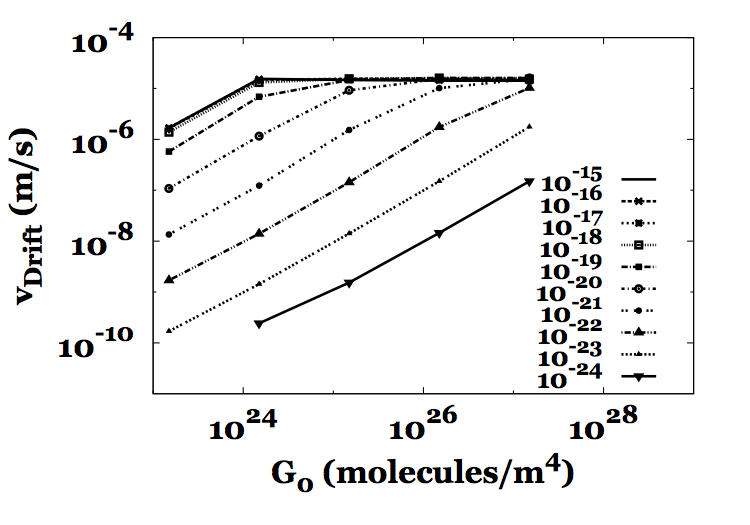
Figure 2: Drift velocity $v_{drift}$ calculated by simulation as a function of the oxygen gradient $G_{0}$ for different values of the aerotaxis coefficient $\alpha$.

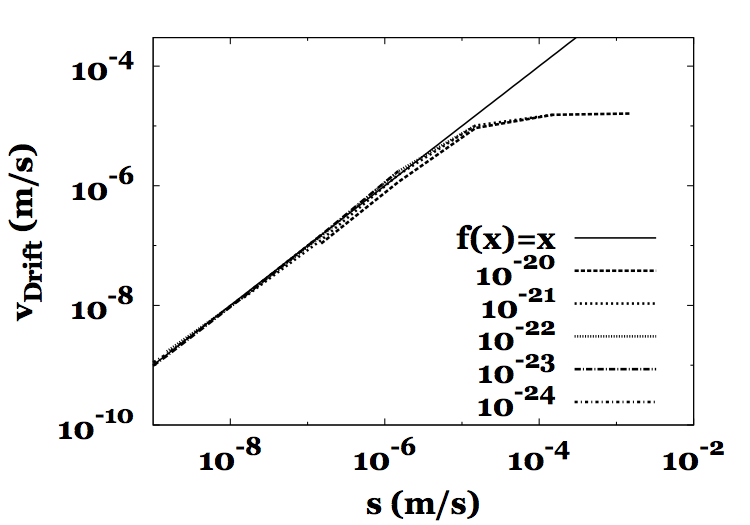
Figure 3: Drift velocity versus $s=G_{0}\alpha v_{0}^{2}\xi/2$. The simulations for different values of $\alpha$ and $G_{0}$ collapse together, and the saturation of the drift velocity is near $G_{0}\alpha v_{0}=1$. $\xi=0.5\ s$.

The model should exhibit a sizeable aerotaxis effect, but should not be affected by spurious effects induced by the plateau in the curve (the drift velocity should remain smaller than the swimming velocity). Since the order of magnitude of the oxygen gradient found in our simulations is at most $10^{26}$ molecules/m⁴, this requires to choose $\alpha<10^{-20}$ m³/molecule.

3.2 Spring constant

An estimation for the “spring constant” $k$ of a matrix “bridge” between bacteria can be deduced from the elastic modulus of the biofilm, that has been measured recently [40]. Assuming that each matrix link between two bacteria has a cross-section of $\pi r_{0}^{2}$ and an equilibrium length of $2r_{0}$, the stress is $\sigma=k\Delta r/(\pi r_{0}^{2})$, where $\Delta r$ is the elongation of the link. Using Hooke’s law for an isotropic medium of Young modulus $Y$, one finds that $\sigma=Y\Delta r/(2r_{0})$. These two relations yield

$$k\sim Y\frac{\pi}{2}r_{0}.$$ (31)

If the measured value of the elastic modulus is used to calculate the spring constant, a problem arises for the numerical simulations, which is due to the multiple time scales present in the problem of biofilm formation. Indeed, considering Eq. (20) applied on two matrix-producer bacteria that are linked by a strained matrix bridge in a fluid at rest, the bridge will relax to its equilibrium length with a characteristic time scale $\tau$ given by:

$$\tau\sim\frac{6\pi\eta r_{0}}{k}=\frac{12\eta}{Y}.$$ (32)

For the Young’s modulus measured in biofilms ($Y=10-10000\,Pa$ [40]), this time scale ranges from $\tau=10^{-3}-10^{-6}$ s. The numerical integration requires a timestep that is much smaller than this time scale in order to properly resolve the dynamics. However, biofilm formation takes several days. Thus, it is extremely difficult to perform simulations of biofilm formation for the physical values of Young’s modulus. Therefore, we have chosen to use much lower values for the spring constant, corresponding to $Y<10^{-1}\,Pa$, which implies that our simulated biofilms are less stiff than in reality. Finally, for the repulsion, the parameter $F_{0}$ is taken to be $10^{-5}\,N$ following similar considerations.

4 Results

We have performed numerical simulations to test the behavior of our model. They show that the model can reproduce all the main stages of biofilm formation. In addition, systematic parametric studies have allowed us to identify the model parameters that have the strongest influence on the biofilm growth dynamics and morphology. Those are the division time of the bacteria $\tau_{d}$ (for the timing of the biofilm nucleation), the value of the bacterial concentration threshold for the phenotypic switch $n_{ph}$, and the value of the spring constant $k$. Moreover, we have tested the influence of bioconvection by comparing simulations with and without coupling to fluid flow.

In the following, we first present a reference simulation in order to provide a description of the typical time evolution of the system. Then, the influence of several model parameters is discussed. All other parameters remain fixed to the values given in Table 3.

4.1 Steps of biofilm formation

In Figures 4, we present a typical sequence of snapshots of the bacterial population and the fluid velocity and oxygen fields, respectively. In the top row of Fig. 4, each bacterium is represented by a colored dot, with motile bacteria in red, the matrix-producer bacteria linked to less than two others bacteria in purple, and matrix-producer bacteria linked to at least two other bacteria in black. Thus, “purple” bacteria are matrix producers that are not (yet) firmly integrated in the biofilm structure, whereas “black” bacteria are part of the connected biofilm tissue. In the middle and lower row, the maps of the fluid velocity and the oxygen concentration corresponding to the same times are displayed.

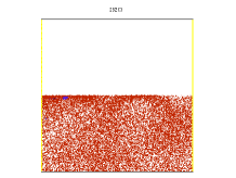
(a)

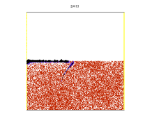
(b)

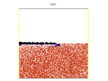
(c)

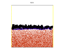
(d)

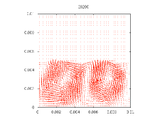
(e)

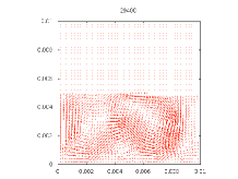
(f)

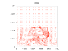
(g)

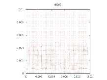
(h)

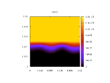
(i)

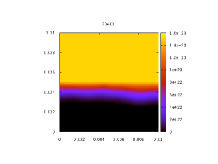
(j)

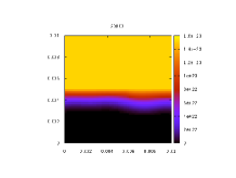
(k)

(l)

Figure 4: The first line shows successive snapshots of the bacterial population (at 7h50 (a), 8h10 (b), 8h20 (c) and 11h10 (d)) during the formation of a biofilm. Second and third lines show respectively the evolution of the fluid velocity and the oxygen. The parameters for the simulation are the one given in table 3.

The initial condition of the simulation is a medium at rest, saturated with oxygen, where 100 planktonic bacteria have been inserted at random positions. The bacteria move around and divide, and the growth and aerotaxis process leads in the course of time to an accumulation of bacteria close to the fluid-air interface as can be seen in Fig. 4a. The density of bacteria close to the interface is higher than the threshold for the onset of bioconvection, and thus there is a pronounced fluid motion that can be seen in Fig. 4e. Due to this convection, the bacterial concentration varies along the surface, and a small cluster of bacteria that have switched from the motile to the matrix-producer phenotype has formed. At a later stage (fig. 4b), the number of bacteria that have switched is significantly higher, and they have started to bind together, thus giving birth to a thin biofilm. In addition, the fluid motion (which is weaker than before, Fig. 4f) has advected toward the bottom of the container a filament of connected matrix-producing bacteria that is reminiscent of the filaments observed in the experiments. Shortly after (Fig. 4c), the biofilm has grown and covers a much larger part of the interface. Finally, after 11h10 (Fig. 4d), the biofilm covers the whole interface and has grown much thicker. Its surface is, in some cases, very irregular and emerges over the level of the water surface. This behavior can be attributed to the fact that we do take into account neither the gravity force that is exerted on the matrix producers that are pushd out of the water by the contact forces, nor the capillary forces. The irregular structure of the bulk is probably due to the fact that our modeling is purely 2D which makes impossible the formation of bicontinuous structures that are more realistic and that would allow swimming bacteria to fill the holes that can be seen in the volume of the biofilm. In addition, there are fewer motile bacteria in the medium (because they have switched to matrix producers), their accumulation at the surface is less pronounced, and consequently the fluid flow is much weaker. The oxygen concentration maps during the biofilm formation (4i, 4j, 4k, 4l) show that there is a strong oxygen gradient close to the interface and a oxygen-depleted region below. They also indicate that the fluid flow induces heterogeneities along the interface (the small bumps in the oxygen concentration profile are clearly correllated with convection rolls). In fig.4l, one should also note that the oxygen concentration map is much more regular than the biofilm itself, which indicates the averaging effect of diffusion.

This sequence gives a good illustration of the biofilm formation process in our model: after a long stage (a few hours) during which bacteria divide and the interplay of oxygen consumption, transport and bacterial motion leads to an accumulation of bacteria on the interface, numerous bacteria switch from the motile to the matrix-producer state within a short time ($\approx$ 10min -1 hour), which gives rise to a thin solid pellicle, the biofilm. It rapidly covers the entire interface. Afterwards, the biofilm grows thicker over a few hours.

Most of the model parameters can be changed over large ranges of values without any qualitative change in the scenario outlined above. However, several parameters have a significant influence on both the morphology of the biofilm and on the time between the beginning of the simulation and the beginning of the biofilm growth, which we will call nucleation time. In the following, we briefly discuss these points, starting with the biofilm morphology and finishing with the nucleation time.

4.2 Morphology of the biofilm

While the rate at which bacteria consume oxygen or divide has little effect on the final biofilm morphology, the value of the threshold for the phenotype switch and the mechanical parameters (elastic constant in the binding force and fluid flow) can dramatically influence the biofilm morphology. In the following, we briefly describe these results.

4.2.1 Effect of the threshold for phenotype switch

In Fig. 5, we present a set of simulations that show how the bacterial concentration at which the phenotype transition occurs ($n_{ph}$) affects the morphology of the biofilm, both with and without bioconvection. Without bioconvection (left column), for small values of the threshold, ($2\times 10^{13}$ bacteria/m³), biofilm nucleation events are homogeneously distributed in the whole medium, and the disconnected pieces of biofilm subsequently grow. For higher values ($4\times 10^{13}$ bacteria/m³), the biofilm is localized close to the interface and consists of chunks of biofilm that are separated by thin fluid channels. This behaviour is present (to a certain extent) up to a threshold of $\approx 2\times 10^{14}$ bacteria/m³. For even higher values, the biofilm is a homogenous layer at the interface. The presence of bioconvection (right column) has little effect on the structures. For high values of the threshold, the biofilm structures are more disconnected with bioconvection than without. For smaller values of the threshold, the matrix producers are organized in structures that are reminiscent of the double convection roll of the flow.

These observations can be partially understood by taking into account the different stages of the growth process. When only a few bacteria are present in the medium, oxygen is supplied by diffusion to the entire system. When the bacterial concentration exceeds a certain value, the oxygen in the medium far from the surface is almost completely consumed, and an oxygen gradient towards the surface develops (and thus an oxygen flux towards the bottom). This triggers the migration of bacteria to the surface. Therefore, both the concentration of the bacteria at the surface and the bacterial density gradient at the surface increase with time. If the transition threshold is low, the transition occurs while the gradients in bacterial concentration are still relatively low, which explains that nucleation occurs in the entire system. On the other hand, when the threshold is high, nucleation occurs only when both the concentration and its gradient are high at the surface, and therefore biofilm formation occurs only in a thin layer close to the surface.

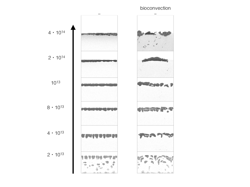
Figure 5: Effect of $n_{ph}$ the threshold of the switch in phenotype on the morphology of the biofilm, with (right column) and without (left column) bioconvection. Here, each snapshot is taken when 10000 of bacteria have switched to the matrix-producer phenotype, and therefore the simulation time is different for each case.

4.2.2 Effect of the spring constant

There is a double effect upon changing the stiffness of the links between bacteria. First, this affects the global elastic properties of the biofilm. Second, having stiffer links implies that they are less likely to be elongated up to a length at which they will break. This means that the plasticity of the biofilm will be much smaller and that it will keep a stronger memory of the growth process than in the case where the connections between bacteria can easily rearrange to accommodate external stresses. This can indeed be observed in Fig. 6. In the case of low elastic constant, the biofilm essentially behaves like a viscous fluid, and inhomogeneities formed during the initial stages of growth tend to be smoothed out. In contrast, for higher elastic constants the growth of the bacterial volume due to matrix production leads to an accumulation of internal elastic stresses in the biofilm and, ultimately, to a deformation of the biofilm reminiscent of a buckling phenomenon as can be seen on the upper right of Fig. 6.

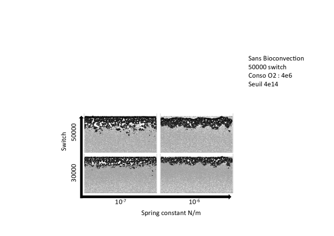
Figure 6: Evolution of the biofilm with different values of spring constant (without fluid flow). The snapshots show the biofilm structure for different times when 30000 and 50000 bacteria have switched into matrix producer phenotype, respectively.

4.3 Nucleation time of the biofilm

Finally, we consider the effects of the model parameters on the time after which the first piece of the biofilm nucleates. Indeed, this nucleation time is a quantity that is largely independent of the criterion selected to define it, due to the rapid growth of the biofilm after its nucleation. Therefore, it can be measured with good precision. Here, we consider that nucleation has taken place when more than 100 bacteria have changed their phenotype.

We first consider the role of the division time of the bacteria. In Fig. 7, the nucleation time is plotted as a function of the division time of the bacteria for different values of the phenotype switch threshold, either with or without flow. In both cases, it is clear that the nucleation time scales approximately linearly with the division time $\tau_{d}$, which is to be expected since the division of bacteria is the elementary step which governs the population increase which in turn triggers the phenotype switch through quorum sensing.

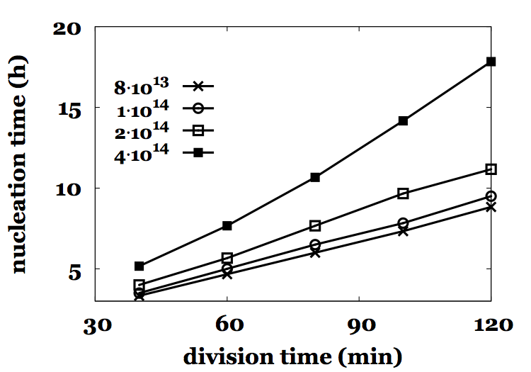
(a)

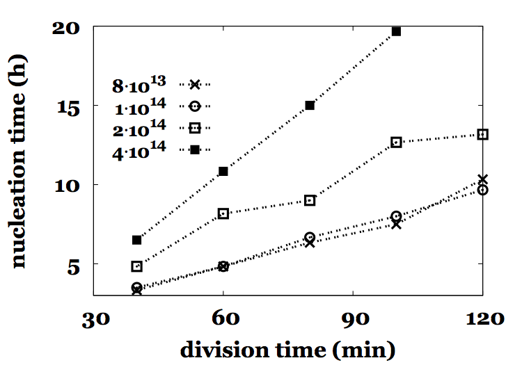
(b)

Figure 7: Nucleation time of the biofilm as a function of the division time $\tau_{d}$ of the bacteria. The different curves correspond to different values of the phenotype switch threshold $n_{ph}$. Figure 7a with convection, figure 7b without convection.

We have also studied the nucleation time as a function of the value of the threshold concentration, both with and without bioconvection. The results of this study are summarized in Fig. 8. In both cases (with and without fluid flow), the nucleation time increases with the threshold value. For small values of the threshold, the nucleation times with and without bioconvection are equal (up to numerical uncertainties), which is expected, since for small values of the threshold, the biofilm appears before the stratification of the medium is sufficient to trigger bioconvection. When the threshold is further increased, biofilm development takes much longer with than without bioconvection. This is due to the mixing effect of convection, which tends to prevent bacterial accumulation close to the interface, and therefore to delay the crossing of the threshold concentration that triggers biofilm formation.

This result should be compared to experiments of biofilm growth in which bioconvection can be precisely controlled without significantly affecting the environment of the bacteria. To our knowledge, such observations have not been reported yet.

Figure 8: Effect of the threshold in the phenotype switch on the nucleation time of the biofilm. Square dots: simulations with fluid flow. Circle dots: without fluid flow.

5 Conclusions and perspectives

We have developed and tested a model of biofilm formation at fluid-air interfaces. The model combines a continuum description of fluid flow and oxygen transport with a description of the bacteria as discrete particles which interact with each other and with their environment. This model, constructed with a minimal set of hypotheses, reproduces all the steps of biofilm formation that are observed in the experiments, particularly an accumulation of bacteria under the fluid-air interface, and bioconvection.

The model relies on several strong simplifying assumptions, particularly concerning the mechanical interactions of bacteria inside the biofilm. Since several of the parameters that characterize bacteria are not well known, quantitative agreement with the experiments cannot be expected. Nevertheless, with the help of the model we have demonstrated that bioconvection can significantly influence the time needed for biofilms to appear. This is an interesting predicition that could be tested in experiements in which bioconvection can be controlled. Furthermore, we have shown that the biofilm morphology is influenced by the balance between the accumulation of bacteria close to the oxygen source and the quorum-sensing mechanism that triggers the transition from motile bacteria to matrix producers. Therefore, it would be extremely important to have more quantitative information about the quorum sensing mechanism in order to improve the model.

Some of the features included in our model are not strictly needed for the understanding of the initial aggregation and nucleation mechanisms of biofilms, but will be necessary to model other phenomena observed in biofilm growth. For instance, after the initial formation of biofilms, they often develop a characteristic wrinkled morphology during maturation. This instability has been explained by the accumulation of mechanical stresses due to the internal growth of the biofilm [40]. The production of a finite volume of matrix in the matrix-producer state included in our model will naturally lead to the accumulation of mechanical energy in the biofilm. Nevertheless, a correct description of the buckling instability would require to develop a coherent treatment for a non-planar fluid-air interface. More precisely, the effect of gravity on the emerging bacteria together with a proper description of capillary effects at the interface should be included. While this is probably feasible our model, we rather believe that such phenomena should be described in the framework of continuum mechanics. In our opinion, promising future lines of research with our model are its extension to three-dimensional systems so that bicontinuous morphologies can appear in the biofilm, and the exploration of changing bacterial behavior.

Appendix A Parameters

Here, we briefly motivate our choices for various model parameters.

• Equation (5) for the oxygen consumption contains two parameters : a rate constant $\gamma$ and a Michaelis constant $K$. The oxygen consumption rate of B. subtilis is $10^{6}$ molecules$/$s$/$bacterium in a saturated culture [25]. It was shown by Martin for Escherichia coli that this rate can vary by one order of magnitude depending on the growth phase of the bacteria [37], with saturated culture corresponding to the minimal oxygen uptake. We suppose that similar variations can occur for B. subtilis, and thus $\gamma$ varies in the range of $10^{6}-10^{7}$ molecules$/$s$/$bacterium. We have used a Michaelis-Menten law to cut off the oxygen consumption at low concentrations; the corresponding Michaelis constant $K$ is unknown. Since observations on E. coli indicate that oxygen is almost completely depleted in concentrated cultures [38], we choose a very small value of $K$ compared to the initial oxygen concentration.

• The integration time constants of the oxygen memory, $\tau_{s}$ and $\tau_{l}$ in equations (8) and (9) are the typical time intervals over which the oxygen concentration is averaged in the internal variables $m_{s}$ and $m_{l}$, respectively. Experimental observations have shown that B. subtilis is able to detect quickly (less than $1\,s$) a sudden variation in oxygen concentration, but adapts to the new average level of oxygen within several seconds [13]. According to these results we take $\tau_{s}=0.1\,s$ and $\tau_{l}=10\,s$.

• The radius $r$ is used for the calculation of the bacterial velocity in Eq. (20). We choose a reference radius $r_{0}=5\,\mu$m (the typical length of B. subtilis when it is in the motile phenotype [25]). For simplicity, we keep the friction coefficient $6\pi\eta r$ constant in Eq. (20) by always using $r=r_{0}$. However, in order to properly calculate the forces between bacteria, Eq. (19), we take into account the growth of the bacterial body size with time through the value of $r_{ij}=r_{i}+r_{j}$. The maximum radius of motile bacteria, $r_{d}$ is chosen as $r_{d}=\sqrt[3]{2}r_{0}\backsimeq 6,3\,\mu m$, which corresponds to a volume twice larger than the reference volume.

• The mass density of bacteria $\rho_{b}$ is needed in Eq. (1) to evaluate the local fluid density for use in the Navier-Stokes equation (4). As already mentioned, several values for this density are quoted in the literature. We take for our simulations a density that is $3\%$ larger than the one of the medium. However, the mature biofilm usually floats on the water, which means that it must also contain some components that are lighter than water. The mass density of the extracellular matrix is actually unknown. To take these observations into account in a simple manner, we use the bacterial “reference volume” $4\pi r_{0}^{3}/3$ for each motile bacterium in the calculation of the total bacterial volume $V_{b}$ in a coarse-grained cell, whereas matrix producers do not contribute.

• To determine the division time of B. subtilis during growth in biofilm conditions, we measure the evolution of the bacterial concentration in the medium over time. The measured division time is around 1h, and we take for the simulations $\tau_{d}=70$ min.

• The propulsion velocity is in the range of $10\,\mu m.s^{-1}$ to $30\,\mu m.s^{-1}$ and slightly depends on the local oxygen concentration [41]. We have taken a constant $v_{0}=20\,\mu m.s^{-1}$ for simplicity.

• The rate of switching from the motile to the matrix-producer phenotype, Eq. (11), contains two constants: the quorum sensing threshold $n_{ph}$ and the rate $1/\tau_{ph}$. We observe in the experiments that the bacterial concentration in the medium at the time of the beginning of the biofilm formation is around $10^{13}$ bacteria$/$m³. The threshold for the change in phenotype must then be higher than this value, because at the water-air interface the bacterial concentration is higher than in the bulk. We explore various values of this parameter in the simulations. The switching time $\tau_{ph}$ sets the rate of switching when concentration threshold is exceeded. We suppose that the transition happens quickly and take $\tau_{ph}=\mbox{$\Delta$t}$.

References

- [1] Steven S Branda, Shild Vik, Lisa Friedman et Roberto Kolter : Biofilms: the matrix revisited. Trends in microbiology, 13(1):20–6, janvier 2005.
- [2] Steven S Branda, Frances Chu, Daniel B Kearns, Richard Losick et Roberto Kolter : A major protein component of the Bacillus subtilis biofilm matrix. Molecular microbiology, 59(4):1229–38, février 2006.
- [3] Sünje Johanna Pamp, Morten Gjermansen et Tim Tolker-nielsen : The Biofilm Matrix: A Sticky Framework. 2007.
- [4] J. William Costerton, Zbigniew Lewandowski, Douglas E Caldwell, Darren R Korber et Hilary M Lappin-scott : Microbial biofilms. Annu. Rev. Microbiol., 1995.
- [5] Paula Watnick et Roberto Kolter : Biofilm , City of Microbes. Journal of bacteriology, 182(10):2675–2679, 2000.
- [6] B D Hoyle et J. William Costerton : Bacterial resistance to antibiotics: the role of biofilms. Prog Drug Res, 37:91–105, 1991.
- [7] B B Finlay et S Falkow : Common themes in microbial pathogenicity revisited. Microbiol. and Mol. Biol. Rev., 61(2):136–169, 1997.
- [8] George O’Toole, Heidi B. Kaplan et Roberto Kolter : Biofilm Formation as Microbial Development. Annu. Rev. Microbiol., pages 49–79, 2000.
- [9] Arnaud Bridier, Dominique Le Coq, Florence Dubois-Brissonnet, Vincent Thomas, Stéphane Aymerich et Romain Briandet : The spatial architecture of Bacillus subtilis biofilms deciphered using a surface-associated model and in situ imaging. PloS one, 6(1):e16177, 2011.
- [10] Hera Vlamakis, Claudio Aguilar, Richard Losick et Roberto Kolter : Control of cell fate by the formation of an architecturally complex bacterial community. Genes & development, 22:945–953, 2008.
- [11] Cristian Picioreanu, J. U. Kreft, Mikkel Klausen, J.A.J. Haagensen, T. Tolker-Nielsen et S. Molin : Microbial motility involvement in biofilm structure formation a 3D modelling study. Water science & technologie, 55(8-9):337–343, 2007.
- [12] Steven S Branda, Eduardo Gonza, Sigal Ben-yehuda, Richard Losick et Roberto Kolter : Fruiting body formation by Bacillus subtilis. PNAS, 891(11), 2001.
- [13] Laurence S Wong, Mark S Johnson, Igor B Zhulin et Barry L Taylor : Role of Methylation in Aerotaxis in Bacillus subtilis. Journal of bacteriology, 177(14):3985–3991, 1995.
- [14] Imre M. Janosi, John O. Kessler et Viktor K Horva : Onset of bioconvection in suspensions of Bacillus subtilis. Physical Review E, 58(4):4793–4800, 1998.
- [15] Kazuo Kobayashi : Bacillus subtilis pellicle formation proceeds through genetically defined morphological changes. Journal of bacteriology, 189(13):4920–31, juillet 2007.
- [16] Brandon Lindley, Qi Wang et Tianyu Zhang : Multicomponent hydrodynamic model for heterogeneous biofilms: Two-dimensional numerical simulations of growth and interaction with flows. Physical Review E, 85(3):031908, mars 2012.
- [17] T J. Pedley et John O. Kessler : Hydrodynamic phenomena in suspensions of swimming microorganisms. Annual reviews fluid mechanics, 1992.
- [18] Cristian Picioreanu, Mark C M van Loosdrecht et J J Heijnen : Mathematical modeling of biofilm structure with a hybrid differential-discrete cellular automaton approach. Biotechnology and bioengineering, 58(1):101–116, 1998.
- [19] J. U. Kreft et J.W.T. Wimpenny : Effect of EPS on biofilm structure and function as revealed by an individual-based model of biofilm growth. Water science and technology : a journal of the International Association on Water Pollution Research, 43(6):135–41, janvier 2001.
- [20] Joao B Xavier, Cristian Picioreanu et Mark C M van Loosdrecht : A framework for multidimensional modelling of activity and structure of multispecies biofilms. Environmental microbiology, 7(8):1085–103, août 2005.
- [21] Erik Alpkvist, Cristian Picioreanu, Mark C M Van Loosdrecht et Anders Heyden : Three-Dimensional Biofilm Model With Individual Cells and Continuum EPS Matrix. Biotechnology and bioengineering, 2006.
- [22] Carey D Nadell, Vanni Bucci, Knut Drescher, Simon a Levin, Bonnie L. Bassler et Joao B Xavier : Cutting through the complexity of cell collectives. Proceedings. Biological sciences / The Royal Society, 280(1755):20122770, mars 2013.
- [23] Damir Lazarevic, Josip Dvornik et Kresmir Fresl : Contact detection algorithm for discrete element analysis. KoG-6, pages 29–40, 2002.
- [24] Pozrikidis C. : Fluid dynamics: theory, computation, and numerical simulation. 2009.
- [25] Luis H. Cisneros, Raymond E. Goldstein et Alex Cronin : The organized melee emergence of collective behavior in concentrated suspensions of swimming bacteria and associated in the graduate college for the degree of doctor of philosophy. Thèse de doctorat, The university of arizona, 2008.
- [26] A.J. Hillesdon, T.J. Pedley et J.O. Kessler : The development of concentration gradients in a suspension of chemotactic bacteria. Bulletin of Mathematical Biology, 57(2):299–344, 1995.
- [27] A. J. Hillesdon et T. J. Pedley : Bioconvection in suspensions of oxytactic bacteria: linear theory. Journal of Fluid Mechanics, 324:223–259, 10 1996.
- [28] Enkeleida Lushi, Raymond E Goldstein et Michael J Shelley : Collective chemotactic dynamics in the presence of self-generated fluid flows. Physical Review E, 86(4):040902, 2012.
- [29] Howard C. Berg : Random walks in biology.
- [30] R M Macnab et D E Koshland : The gradient-sensing mechanism in bacterial chemotaxis. Proceedings of the National Academy of Sciences of the United States of America, 69(9):2509–2512, septembre 1972.
- [31] J E Segall, S M Block et Howard C. Berg : Temporal comparisons in bacterial chemotaxis. Proceedings of the National Academy of Sciences of the United States of America, 83(23):8987–91, décembre 1986.
- [32] Evelyn F Keller et L E E A Segelf : Model for Chemotaxis. Journal of theoretical biology, pages 225–234, 1971.
- [33] Mark J. Schnitzer : Theory of continuum random walks and application to chemotaxis. Phys. Rev. E, 48:2553–2568, Oct 1993.
- [34] Bonnie L. Bassler et Richard Losick : Bacterially speaking. Cell, 125(2):237–46, avril 2006.
- [35] Yunrong Chai, Frances Chu, Roberto Kolter et Richard Losick : Bistability and biofilm formation in Bacillus subtilis. Molecular microbiology, 67(2):254–63, janvier 2008.
- [36] Daniel López et Roberto Kolter : Extracellular signals that define distinct and coexisting cell fates in Bacillus subtilis. FEMS microbiology reviews, 34(2):134–49, mars 2010.
- [37] B Y Donald S Martin : The oxygen consumption of escherichia coli during the lag and logarithmic phases of growth. Journal of general physiology, (1927):691–708, 1932.
- [38] Carine Douarche, Axel Buguin, Hanna Salman et Albert Libchaber : E. Coli and Oxygen: A Motility Transition. Physical Review Letters, 102(19):2–5, 2009.
- [39] Wolgang Alt : Biased walk models for chemotaxis and related diffusion approximations. Journal of mathematical biology, 177:147–177, 1980.
- [40] Miguel Trejo, Carine Douarche, Virginie Bailleux, Christophe Poulard, Sandrine Mariot, Christophe Regeard et Eric Raspaud : Elasticity and wrinkled morphology of Bacillus subtilis pellicles. Proceedings of the National Academy of Sciences of the United States of America, 110(6):2011–2016, janvier 2013.
- [41] Andrey Sokolov et Igor Aranson : Physical Properties of Collective Motion in Suspensions of Bacteria. Physical Review Letters, 109(24):248109, décembre 2012.