Bilayer honeycomb lattice with ultracold atoms: Multiple Fermi surfaces and incommensurate spin density wave instability

Abstract

We propose an experimental setup using ultracold atoms to implement a bilayer honeycomb lattice with Bernal stacking. In presence of a potential bias between the layers and at low densities, Fermions placed in this lattice form an annular Fermi sea. The presence of two Fermi surfaces leads to interesting patterns in Friedel oscillations and RKKY interactions in presence of impurities. Furthermore, a repulsive fermion-fermion interaction leads to a Stoner instability towards an incommensurate spin-density-wave order with a wave vector equal to the thickness of the Fermi sea. The instability occurs at a critical interaction strength which goes down with the density of the fermions. We find that the instability survives interaction renormalization due to vertex corrections and discuss how this can be seen in experiments. We also track the renormalization group flows of the different couplings between the fermionic degrees of freedom, and find that there are no perturbative instabilities, and that Stoner instability is the strongest instability which occurs at a critical threshold value of the interaction. The critical interaction goes to zero as the chemical potential is tuned towards the band bottom.

I Introduction

The presence of multiple Fermi surfaces is a common and recurring theme in electronic systems, occuring in systems as varied as simple metals like Ti or Cr, to doped topological insulators like Nb doped $\text{Bi}_{2}\text{Se}_{3}$ dopedtopo to heavy fermion compounds like $\text{UPt}_{3}$ UPT3 to recently discovered Iron based high temperature superconductors FEAS ; pnictide . In some cases, they simply add an additional quantum number to the low energy theory and change the low energy behavior of the system only in quantitative aspects. In more complicated systems like iron- based superconductors  pnictide ; FEAS , the presence of almost nested Fermi surfaces are believed to play a more complex role. The interaction between electrons on the different Fermi surfaces leads to strong spin fluctuations at the nesting wave vector, which in turn drives a superconducting instability in the system. It is, therefore, interesting to study the complex interplay of multiple Fermi surfaces and interactions in a system where one can change both the interaction scales and the shape or size of the Fermi surfaces in a controllable way.

Graphene and its few layer counterparts have emerged as two-dimensional (2D) systems where the shape of the dispersion as well as the size of the Fermi surface can be tuned controllably by using gate voltages in various configurations. Bilayer graphene, which consists of two layers of carbon atoms arranged in a honeycomb lattice in a Bernal AB stacking arrangement is an interesting platform to study the effects of electron-electron interactions in 2D chiral systems blg1 ; blg2 . The tunability of the carrier density by gating the system, together with the low energy bands with quadratic dispersion, provide access to strongly interacting regimes at low carrier density. The strong interaction can lead to different symmetry broken ground states vafek ; macdonald and non-Fermi liquid behavior nfl ; sensarma1 at the charge neutrality point in this system. However, in real materials, some of these effects may be hard to observe due to the presence of strong Coulomb and short-range impurities disorder which lead to the formation of puddles of positively and negatively charged regions even in a sample that is charge neutral on average.

In biased bilayer graphene, an effective electric field between the layers breaks the layer symmetry and the potential difference between the layers gaps out the low lying bands, with a tunable band gap which can be controlled by the gate voltages bbilayer_expt . More recently, it has been proposed that domain walls between $A-B$ and $B-A$ type biased bilayer graphene can sustain a pair of topological edge states with different valley quantum numbers bilayer_topo . In a homogeneous biased bilayer graphene, the low energy dispersion of the bands has a sombrero (Mexican hat) like dispersion, with the band bottom forming a circle in the Brillouin zone. If the chemical potential is tuned to lie in the well of the Mexican hat, the Fermi sea takes the shape of an annulus. The presence of 2 Fermi surfaces, a diverging density of states at the band bottom, and strong electronic correlations are expected to lead to a wide range of interesting phenomena in this system. However, in material bilayer graphene, the depth of the Mexican hat well is comparable to the energy scale of disorder in current samples  bbilayer_expt ; disorder , and thus the phenomena due to the presence of 2 Fermi surfaces will be smeared out in these systems.

Ultracold atoms have emerged in recent years as a new platform to study interacting quantum many body systems Bloch_review ; Esslinger_review . The precise knowledge of tunable Hamiltonian parameters and absence of disorder in these systems has made them ideal for controlled access to various phases of matter like Mott insulators, superfluids etc. and the phase transitions between them Greiner . Thus, an implementation of the biased Bernal-stacked bilayer honeycomb lattice with ultracold atomic systems will provide the opportunity to study the interplay of multiple Fermi surfaces and interaction, since each can be individually controlled in this system. These systems are ideal for probing the physics described above as one can use the tunability of parameters to make the sombrero well deeper, and the cleanliness of the system precludes disorder washing out the phenomenology.

In this paper, we propose an experimental setup of ultracold atoms to implement a Bernal-stacked bilayer honeycomb lattice with a potential bias between the layers and show that there is a wide range of experimentally achievable parameters which allow the observation of the effects of the annular Fermi sea with two Fermi surfaces. We show that, at low densities of ultracold fermions, the presence of two Fermi surfaces leads to interesting patterns of density oscillations (Friedel oscillations) in the presence of impurities. Thus the presence of the annular sea and its consequences can be captured even for non-interacting fermions. In ultracold atomic systems the fermions interact through a short-range interaction characterized by an s-wave scattering length in the continuum. This leads to a Hubbard model on the lattice, where the sign of the interaction can be tuned through a Feshbach resonance. We note that since we are interested in a lattice model close to half-filling, the usual concerns of rapid atom loss in continuum repulsive systems do not play a role in our implementation, and the interacting system is stable to major atom loss. Repulsive interactions between fermions on the biased bilayer honeycomb lattice lead to an instability towards an incommensurate spin-density-wave (SDW) state with a wave vector which is equal to the thickness of the Fermi sea. We find that this Stoner instability survives the manybody renormalization of the interaction with small changes in the critical coupling. A renormalization group analysis of the problem at low energies shows that there are no perturbative instabilities in this system which can overshadow the Stoner instability (which is a threshold phenomenon, as it requires a finite interaction strength); and the SDW is the strongest instability within a finite threshold mean-field analysis among competing orders. We discuss several possible experimental signatures of the new order. We note that a prediction of Stoner instability at $q=0$ exists for biased bilayer graphene bbilayer_ferro , but this is different from our prediction of an incommensurate spin-density wave in cold atoms with short range interactions.

The rest of the paper is organized as follows: (i) In Sec.  II, we first describe our proposal for experimental implementation of the biased bilayer honeycomb lattice with Bernal stacking using ultracold atoms. We then describe the band dispersion in such a system and relate these to the optical lattice parameters using a band structure calculation. We show that there is a wide range of experimental parameters where the effects of the annular Fermi sea can be seen and comment on the optimal parameters for the experiments. (ii) In Sec.  III, we consider the static polarizability of a system of non-interacting fermions in this lattice, which governs its response to potential perturbations. We calculate this using (a) the detailed band dispersion and the band wavefunctions, and (b) a one-band approximate dispersion, which provides analytic insight into the problem. We find that there are three singularities of this function, which lead to the presence of three wave vectors in the Friedel oscillations in these systems. (iii) In Sec.  IV, we consider the possibility of an incommensurate spin-density wave instability in a system of repulsively interacting fermions in this lattice. We first consider the simple Stoner picture, where a spin-density wave instability occurs at a critical coupling monotonically decreasing with density. We further show that the Stoner instability is almost unchanged if we go beyond Stoner approximation and include vertex corrections which incorporate reduction of the interaction due to many body effects. (iv) In Sec.  V, we consider the possibility of competing instabilities within a renormalization group framework. We show that in this system, there is no perturbative instability which overtakes the spin density wave instability mentioned above. Furthermore, within mean field analysis, the Stoner instability is the strongest among different orders quadratic in the Fermi fields. This strengthens the case for the SDW to be the leading instability in the system. We finally conclude in Sec.  VI with a discussion and outlook on this problem.

II Bilayer Honeycomb lattice with cold atoms

Ultracold atoms in optical lattices, where a periodic potential is created by standing waves formed by lasers, have been used to study strongly interacting manybody systems in a controllabel way Bloch_review . In this section, we will first present a scheme to implement biased Bernal stacked bilayer honeycomb lattice with ultracold atomic systems in optical lattices. We will then look at the dependence of the important tight binding parameters on the optical lattice parameters using a band structure calculation. From the band dispersion, we will extract the range of tight binding parameters and chemical potentials which are optimal for observing the effects of the two Fermi surfaces and the consequent Stoner instability. Finally, we will make the connection to the optical lattice parameters through our band structure calculation and show that there is a wide range of experimentally accessible parameters where the effects of the presence of two Fermi surfaces can be seen.

II.1 The Optical Lattice

A honeycomb lattice can be formed by interfering three coplanar laser beams propagating at an angle $\pm\pi/3$ with respect to each other  Demler_Kitaev_2003 . Variants of this scheme has been experimentally implemented Taruell_Honeycomb to observe the low energy Dirac quasiparticles. While there are proposals to create A-A bilayers bilayer_AB_prop ,

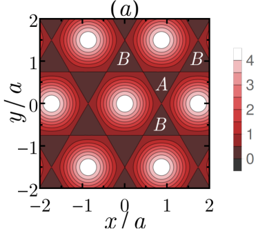
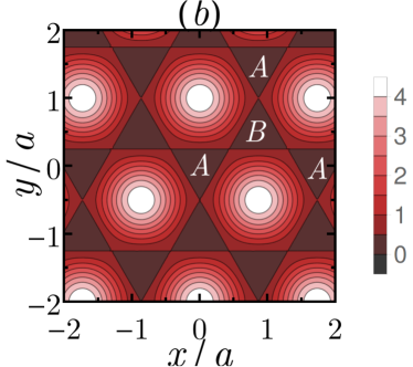
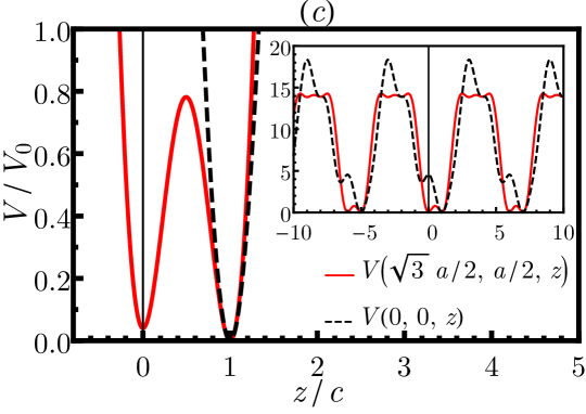
Figure 1: Color plots of the optical lattice potential (in units of $V_{0}$) in the $x-y$ plane at (a) $z=0$ and (b) $z=c$. (c) The potential as a function of $z$ at $(\sqrt{3}/2,1/2)a$ (solid red line) showing A-B stacking and at $(0,0)$ (dashed black line) showing potential well in only one layer. Inset: The potential profile on a larger $z$ scale, showing the almost decoupled bilayers.

we propose here a simple scheme of generating the Bernal stacked bilayer honeycomb lattice using five lasers with the potential

$$V(\mathbf{r}) = V_{0}[\cos(\mathbf{p_{1}}\cdot\mathbf{r})+\cos(\mathbf{p_{2}}\cdot\mathbf{r})+\cos(\mathbf{p_{3}}\cdot\mathbf{r})+\frac{3}{2}]$$

$$-\alpha V_{0}\left[\cos\left(\mathbf{p_{4}}\cdot\mathbf{r}-\phi_{1}\right)-\frac{1}{6}\cos\left(\mathbf{p_{5}}\cdot\mathbf{r}-\phi_{2}\right)-\frac{\sqrt{3}}{2}\right]$$

where $\mathbf{p_{1}}=(\frac{2\pi}{\sqrt{3}a},\frac{2\pi}{3a},-\frac{2\pi}{3c})$, $\mathbf{p_{2}}=(-\frac{2\pi}{\sqrt{3}a},\frac{2\pi}{3a},-\frac{2\pi}{3c})$ and $\mathbf{p_{3}}=(0,-\frac{4\pi}{3a},\frac{4\pi}{3c})$ produces a honeycomb lattice in the $x-y$ plane with lattice constant $a$, whose origin is shifting with $z$ in such a way that it results in $A-B$ stacking with intralayer distance c. These three layers however create a 2D pattern whose origin is continuously shifting with $z$. In order to pick out the correct $x-y$ planes corresponding to the bilayer, the last two lasers, with $\mathbf{p_{4}}=(0,0,\frac{\pi}{3c})$, $\mathbf{p_{5}}=(0,0,\frac{\pi}{c})$, $\phi_{1}=\frac{\pi}{6}$ and $\phi_{2}=\frac{\pi}{2}$, create a superlattice in the $z$ direction and picks up the planes $z=0$ and $z=c$, producing the Bernal stacked bilayer. The full laser arrangement actually creates a superlattice of bilayers, separated by a distance $6c$, but the large distance between successive bilayers result in a system of decoupled Bernal stacked bilayer honeycomb lattice. In addition, a bias $\Delta$ can be created between the planes either by a trapping potential or by application of a weak laser with wavelength $2c$.

The potential in the $x-y$ plane at $z=0$ and $z=c$ are plotted in Fig 1 (a) and (b), which shows the shifted honeycomb pattern in the two layers. The potential as a function of $z$ is plotted in Fig 1(c) for in-plane location $(\sqrt{3},1)\frac{a}{2}$ (solid red line), where $A$ and $B$ sublattices lie above each other, and for the location $(0,0)$, where there is a potential well ($B$ sublattice) in only one plane (dashed black line). The inset shows the stack of decoupled bilayers, repeated with period $6c$.

II.2 Biased bilayer and annular Fermi sea

The bilayer honeycomb lattice has four sites in its unit cell described by the sublattice (A and B) and layer ($1$ and $2$) indices. The tight-binding Hamiltonian tight_binding consists of nearest neighbor in-plane tunneling $\gamma_{0}$ and an interlayer tunneling $\gamma_{1}$ between $A_{1}$ and $B_{2}$ sites footnote1 . $\gamma_{0}$, which depends on $a$ and $V_{0}$, is known to follow coldatom_bandparam_1 ; coldatom_bandparam_2 , $\gamma_{0}/E_{R}=1.16(V_{0}/2E_{R})^{0.95}exp(-1.634\sqrt{V_{0}/2E_{R}})$ coldatom_bandparam_2 ; footnote2 (with $E_{R}=8\pi^{2}\hbar^{2}/27ma^{2}$). $\gamma_{1}$ depends on $c$, $V_{0}$ and $\alpha$. Fig 2 shows the variation of $\gamma_{1}$ obtained from a band structure calculation for different values of $c/a$ and $\alpha$ Wannier . Since the parameters $c/a$ and $\alpha$ are tunable in a cold atom setting, the ratio $\gamma_{1}/\gamma_{0}$ can be tuned over a large range in the cold-atom system. An independently tunable bias between the layers, $\Delta$, can be added to gap out the single particle spectrum.

The tight binding band theory is written in the basis $\psi_{k}=(c_{A1k},c_{B1k},c_{A2k},c_{B2k})$  blg_review as $H=\sum_{k}\psi^{\dagger}_{k}H_{k}\psi_{k}$ where,

$$H_{k}=\left(\begin{array}[]{cccc}\frac{\Delta}{2}&-\gamma_{0}f({\bf k})&0&-\gamma_{1}\\ -\gamma_{0}f({\bf k})^{*}&\frac{\Delta}{2}&0&0\\ 0&0&-\frac{\Delta}{2}&-\gamma_{0}f({\bf k})\\ -\gamma_{1}&0&-\gamma_{0}f({\bf k})^{*}&-\frac{\Delta}{2}\end{array}\right).$$ (2)

and $f({\bf k})=e^{ik_{y}a/\sqrt{3}}+2e^{-ik_{y}a/2\sqrt{3}}\cos{k_{x}a/2}$. $\gamma_{0}$ is the in-plane nearest neighbour hopping,$\gamma_{1}$ is the c-axis hopping between the $A$ and $B$ lattice sites that lie on top of each other ($A1$ and $B2$) and $\Delta$ is the potential bias between the layer. Here $\gamma_{0}$ and $\gamma_{1}$ are much larger than $\gamma_{3}$ (hopping between $B1$ and $A2$), and $\gamma_{4}$ (hopping between $A1$ and $A2$), which are neglected in our calculation blg2 . Near the Dirac points of the in-plane Hamiltonian, the structure factor $f(\mathbf{K}^{\pm}+{\bf q})\simeq-v_{F}(\pm q_{x}-iq_{y})$, and hence the Hamiltonian in the two inequivalent valleys is

$$H_{k}=\left(\begin{array}[]{cccc}\frac{\Delta}{2}&v_{F}ke^{-i\theta_{k}}&0&-\gamma_{1}\\ v_{F}ke^{i\theta_{k}}&\frac{\Delta}{2}&0&0\\ 0&0&-\frac{\Delta}{2}&v_{F}ke^{-i\theta_{k}}\\ -\gamma_{1}&0&v_{F}ke^{i\theta_{k}}&-\frac{\Delta}{2}\end{array}\right).$$ (3)

Here $v_{F}=\sqrt{3}a\gamma_{0}/2$ is the Fermi velocity and $\theta_{k}$ is the azimuthal angle in the $\vec{k}$ space. The dispersion  tight_binding consists of four bands

$$\pm E^{\sigma}_{\bf k} = \pm\left[\Delta^{2}/4+\gamma_{1}^{2}/2+v_{F}^{2}k^{2}\right.$$

$$\left.+\sigma\sqrt{v_{F}^{2}k^{2}(\Delta^{2}+\gamma_{1}^{2})+\gamma_{1}^{4}/4}\right]^{1/2}$$

where $\sigma=\pm 1$. The wavefunctions corresponding to these bands are given by

$$\phi_{+}^{\sigma}(k) = [u^{\sigma}_{{\bf k}},v^{\sigma}_{{\bf k}}e^{i\theta_{{\bf k}}},w^{\sigma}_{{\bf k}}e^{-i\theta_{{\bf k}}},x^{\sigma}_{{\bf k}}]$$ (5)

$$\phi_{-}^{\sigma}(k) = [-x^{\sigma}_{{\bf k}},w^{\sigma}_{{\bf k}}e^{i\theta_{{\bf k}}},-v^{\sigma}_{{\bf k}}e^{-i\theta_{{\bf k}}},u^{\sigma}_{{\bf k}}]$$

where $\theta_{k}$ is the azimuthal angle in the momentum space, and $u^{\sigma}_{{\bf k}}=\cos\chi^{\sigma}_{{\bf k}}\cos\alpha^{\sigma}_{{\bf k}}$, $v^{\sigma}_{{\bf k}}=\cos\chi^{\sigma}_{{\bf k}}\sin\alpha^{\sigma}_{{\bf k}}$, $w^{\sigma}_{{\bf k}}=\sin\chi^{\sigma}_{{\bf k}}\sin\beta^{\sigma}_{{\bf k}}$ and $x^{\sigma}_{{\bf k}}=\sin\chi^{\sigma}_{{\bf k}}\cos\beta^{\sigma}_{{\bf k}}$, with

$$\alpha^{\sigma}_{{\bf k}} = \tan^{-1}\frac{v_{F}k}{E^{\sigma}_{{\bf k}}-\Delta/2}$$ (6)

$$\beta^{\sigma}_{{\bf k}} = \tan^{-1}\frac{v_{F}k}{E^{\sigma}_{{\bf k}}+\Delta/2}$$

$$\chi^{\sigma}_{{\bf k}} = \tan^{-1}\frac{(v_{F}^{2}k^{2}-(E^{\sigma}_{{\bf k}}-\Delta/2)^{2})\sqrt{(E^{\sigma}_{{\bf k}}+\Delta/2)^{2}+v_{F}^{2}k^{2}}}{\gamma_{1}(E^{\sigma}_{{\bf k}}+\Delta/2)\sqrt{(E^{\sigma}_{{\bf k}}-\Delta/2)^{2}+v_{F}^{2}k^{2}}}.$$

For small momenta around the Dirac points, the $\sigma=+1$ bands are high energy bands, gapped out on a scale of $(\Delta^{2}/4+\gamma_{1}^{2})^{1/2}$ and we focus on the two low energy bands ($\sigma=-1$). The bands have a sombrero like dispersion with a local maxima at $k=0$ of height $\Delta/2$ and a band minimum on a circle of radius $k_{0}=\frac{\Delta}{2v_{F}}\left[(\Delta^{2}+2\gamma_{1}^{2})/(\Delta^{2}+\gamma_{1}^{2})\right]^{1/2}$ with the energy at the band bottom given by $E_{0}=\frac{\Delta/2}{\sqrt{1+\Delta^{2}/\gamma_{1}^{2}}}$.

If the chemical potential $\mu$ can be tuned to lie within the well of the mexican hat, of depth $V_{dip}=\frac{\Delta}{2}(1-(1+\Delta^{2}/\gamma_{1}^{2})^{-1/2})$, the Fermi sea is annular in shape, with outer and inner radii given by $v_{F}^{2}k_{\pm}^{2}=\frac{\Delta^{2}}{4}+\mu^{2}\pm\sqrt{\mu^{2}(\Delta^{2}+\gamma_{1}^{2})-\frac{\gamma_{1}^{2}\Delta^{2}}{4}}$.

Figure 2: The dependence of the interplanar coupling $\gamma_{1}$ on the lattice parameter $V_{0}$ for different values of $c/a$ for (a) $\alpha=4$ and (b) $\alpha=8$.

Near the Dirac points, the low energy band dispersion takes the shape of a mexican hat, and one can use an approximate quartic dispersion $\epsilon_{k}=\epsilon_{0}(k^{2}-k_{0}^{2})^{2}+\delta$ to reproduce the main features of the system analytically. The parameter $k_{0}$ can be chosen to coincide with the location of the band bottom, $k_{0}=\frac{\Delta\sqrt{\Delta^{2}+2\gamma_{1}^{2}}}{2v_{F}\sqrt{\Delta^{2}+\gamma_{1}^{2}}}$. For the other two parameters the choice $\epsilon_{0}=\frac{V_{dip}}{k_{0}^{4}}$ and $\delta=\frac{\Delta}{2\sqrt{1+\Delta^{2}/\gamma_{1}^{2}}}$ matches the dispersion at $k=0$ and $k=k_{0}$ and fixes the depth of the mexican hat, as well as the energy at the band bottom. Fig. 3(a) demonstrates a comparison between the detailed band dispersion and the approximate band dispersion in the relevant region of the Brillouin zone for the parameter values $\gamma_{0}=\gamma_{1}=\Delta$.

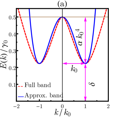
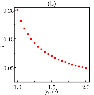
Figure 3: (a) The sombrero-like low energy dispersion of the actual band and the approximate band for $\gamma_{1}=\gamma_{0}=\Delta$. The figure shows how the parameters of the approximate band are obtained from the full dispersion(b) The ratio $r$ corresponding to the normalized density within the well of the sombrero of height $V_{dip}$ as a function of $\gamma_{0}/\Delta$. $\gamma_{0}/\Delta$ corresponds to the largest $r\sim 0.25$

II.3 Choice of band parameters

For bilayer graphene the values of the tight binding parameters are fixed, a standard profile being $\gamma_{1}\simeq 0.4\text{eV}$, $v_{F}=10^{6}\text{m/s}$ and a typical bias voltage $\Delta\simeq 10-100\text{meV}$ blg2 . However for the bilayer honeycomb optical lattice there is a flexibility in choosing the parameters of interest by tuning the laser profiles. The two main considerations which define the set of optimal parameters are (i) the depth of the Mexican hat potential should be as large as possible within other experimental constraints. This provides a large temperature window over which the effects of the ring-shaped Fermi sea can be seen clearly. (ii) the width of the Mexican hat dip (in momentum space) should be as large as possible. A wide well implies that a large density change corresponds to a small chemical potential change and hence the acceptable error within which densities need to be fixed in experiments increases.

The phenomena associated with annular Fermi sea would be easier to observe if the well of the sombrero is deeper (less affected by thermal fluctuations) and wider (a large change in the experimentally controlled density results in a relatively small change in $\mu$). While this implies large $\Delta/\gamma_{1}$ and large $\Delta/\gamma_{0}$ respectively, $\Delta/\gamma_{1}$ is bounded by the constraint that the bias cannot be larger than the c-axis bandwidth. $\Delta/\gamma_{0}$ is constrained by the fact that for $\Delta/\gamma_{0}\gg 1$, the dispersion along the line connecting the two valleys is very flat and the description in terms of populating the individual sombreros around the different valleys do not remain valid. We define $r$ to be the ratio of the density at which the annulus shaped Fermi surface disappears, to the area of the Brillouin zone. We find that $r$ is controlled by $\gamma_{0}/\Delta$ and keeps increasing with decreasing $\gamma_{0}/\Delta$, as shown in Fig. 3(b). The tradeoff is optimized for $\Delta=\gamma_{0}=\gamma_{1}$ which corresponds to $r\sim 0.25$. We note that the independent tunability of $V_{0}$, $a$, $c$ and $\alpha$ provides a wide latitude in choosing experimental parameters.

The Van der Waals interaction between the fermions, described by a scattering length $a_{s}$, leads to a local Hubbard interaction $H_{int}=U\sum_{i\tau}n_{i\tau\uparrow}n_{i\tau\downarrow}$, where $\tau$ denotes the sublattice and layer indices. In the deep lattice limit, $U=\frac{4\pi a_{s}\hbar^{2}}{27a^{2}cm}\left(\frac{2\pi^{2}V_{0}}{E_{R}}\right)^{3/4}\sqrt{\frac{\alpha}{\sqrt{3}}+8}$, and it can be tuned by changing $a_{s}$, $V_{0}$ or $\alpha$. This can be used, for example, to quench the system across the critical interaction strength corresponding to the Stoner instability, which we will discuss in the later part of this paper.

Having shown the wide range of available experimental parameters, we now focus on the signatures of the sombrero type dispersion, especially of the presence of two Fermi surfaces, in the static susceptibility of this system.

III Response in Non-Interacting System

The response of the fermions to potential perturbations is governed by the susceptibility

$$\Pi^{0}({\bf q},\omega)=-\sum_{ss^{\prime}{\bf k}}\frac{n_{F}(sE_{\bf k})-n_{F}(s^{\prime}E_{{\bf k}+{\bf q}})}{\omega+sE_{\bf k}-s^{\prime}E_{{\bf k}+{\bf q}}}F^{ss^{\prime}}({\bf k},{\bf q})$$ (7)

with $F^{ss^{\prime}}({\bf k},{\bf q})=|\phi_{s}^{\dagger}({\bf k})\phi_{s^{\prime}}({\bf k}+{\bf q})|^{2}$, where $\phi_{s}(k)$ is the band eigenfunction. It is then clear that the wavefunction overlaps $F^{ss^{\prime}}({\bf k},{\bf k}+{\bf q})$ can be written in terms of the functions $u_{\bf k}$,$v_{\bf k}$,$w_{\bf k}$ and $x_{\bf k}$ defined above,

$$F^{++}({\bf k},{\bf k}^{\prime}) =(uu^{\prime}+xx^{\prime})^{2}+v^{2}v^{\prime 2}+w^{2}w^{\prime 2}+2(uu^{\prime}+xx^{\prime})(vv^{\prime}+ww^{\prime})\cos\Delta\theta+2vv^{\prime}ww^{\prime}\cos 2\Delta\theta$$

$$F^{+-}({\bf k},{\bf k}^{\prime}) =(xu^{\prime}-ux^{\prime})^{2}+v^{2}w^{\prime 2}+w^{2}v^{\prime 2}+2(xu^{\prime}-ux^{\prime})(vw^{\prime}-wv^{\prime})\cos\Delta\theta-2vv^{\prime}ww^{\prime}\cos 2\Delta\theta$$ (8)

where we have used a shortened notation ${\bf k}^{\prime}={\bf k}+{\bf q}$, and the angle between ${\bf k}$ and ${\bf k}+{\bf q}$, $\Delta\theta$, is given by $\cos\Delta\theta=\frac{k+q\cos\theta}{|{\bf k}+{\bf q}|}$, $\theta$ being the angle between ${\bf k}$ and ${\bf q}$. The index $\sigma=-1$ is dropped from the functions for notational brevity. We note the presence of both $\cos\Delta\phi$, reminiscent of the chiral factors of graphene and $\cos 2\Delta\phi$, reminiscent of the chiral factors of bilayer graphene, in the expression for the overlap. This implies that the backscattering is not completely suppressed in this case as in graphene. However In the limit $\gamma_{1}\rightarrow 0$ we recover the suppression of backscattering present in graphene, while in the $\Delta\rightarrow 0$ limit we recover the enhancement of backscattering as found in bilayer graphene, and by tuning parameters we can smoothly go from one limit to the other.

The static susceptibility at $T=0$, $\Pi^{0}({\bf q},0)$, is plotted as a function of $q$ in Fig. 4 (a-c) for decreasing values of $\gamma_{1}$ (blue dashed line), with $\mu=0.15V_{dip}$. $\Pi_{0}(q)$ has derivative singularities at $q=\delta k=k_{+}-k_{-}$ and $q=2k_{\pm}$, with the strongest singularity occurring at $q=\delta k$. The $2k_{\pm}$ singularities weaken as $\gamma_{1}$ decreases and the system approaches the limit of two decoupled graphene layers, where the absence of backscattering leads to a weaker singularity  Euyhyeon . The singularities in the susceptibility arise from phase space restrictions whenever the Fermi surface shifted by the vector ${\bf q}$ touches the original Fermi surface. At $q=k_{+}+k_{-}$, the inner ring of the shifted Fermi surface touches the outer ring of the original Fermi surface, while the outer ring of the shifted Fermi surface touches the inner ring of the original Fermi surface. The singular contributions from these cancel each other and hence, although backscattering connects fermions on the outer Fermi surface to those on the inner Fermi surface at $q=k_{+}+k_{-}$, there is no singularity at this wave vector. A similar situation arises when $q=\delta k$, but in this case the singularities reinforce each other. To obtain analytic insight into the behaviour of the susceptibility, we work with one band model $\epsilon_{k}=\epsilon_{0}(k^{2}-k_{0}^{2})^{2}+\delta$, where $\epsilon_{0}$ and $\delta$ are chosen to match the low energy dispersion of the actual conduction band. The static susceptibility within this approximation is given by

$$\Pi^{0}({\bf q},i0^{+})=-\sum_{k}\frac{n_{F}(\xi_{k})-n_{F}(\xi_{k+q})}{\epsilon_{k}-\epsilon_{k+q}+i0^{+}}$$ (9)

where $\xi_{k}=\epsilon_{k}-\mu$ and the $i0^{+}$ from the analytic continuation is kept explicitly as it will play a vital role later. At $T=0$, this can be reduced to

$$\Pi^{0}({\bf q},0^{+})=-\frac{1}{2\pi^{2}\epsilon_{0}}\mathcal{R}\left[\int^{k_{+}}_{k_{-}}kdk\int^{\pi}_{-\pi}d\phi\left(\frac{1}{i0^{+}+(k^{2}-k_{0}^{2})^{2}-(k^{2}+2kq\cos\phi+q^{2}-k_{0}^{2})^{2}}\right)\right]$$ (10)

Rewriting the denominator as $(2kq\cos\phi+x+y)(2kq\cos\phi+x-y)$, with $x=k^{2}+q^{2}-k_{0}^{2}$ and $y=\sqrt{(k^{2}-k_{0}^{2})^{2}+i0^{+}}$, the angular integral gives

$$\Pi^{0}({\bf q},0^{+}) = -\frac{1}{2\pi\epsilon_{0}}\mathcal{R}\left[\int^{k_{+}}_{k_{-}}kdk\frac{1}{y(k)}\left[\frac{1}{\sqrt{(k+q)^{2}-k_{0}^{2}+y(k)}\sqrt{(k-q)^{2}-k_{0}^{2}+y(k)}}\right.\right.$$ (11)

$$\left.\left.-\frac{1}{\sqrt{(k+q)^{2}-k_{0}^{2}-y(k)}\sqrt{(k-q)^{2}-k_{0}^{2}-y(k)}}\right]\right]$$

After careful analytic continuation, $\frac{1}{\sqrt{(k^{2}-k_{0}^{2})^{2}+i0^{+}}}$ can be replaced by ${\cal P}\left[\frac{1}{|k^{2}-k_{0}^{2}|}\right]-i\frac{\pi}{2}\delta(k^{2}-k_{0}^{2})$. Separating the real and imaginary parts of the two terms within the parenthesis of (11) as $A^{\prime}(k)+iA^{\prime\prime}(k)$, we get, $\Pi^{0}({\bf q},0^{+})=-\frac{1}{2\pi\epsilon_{0}}\left[\mathcal{P}\int^{k_{+}}_{k_{-}}kdk\frac{1}{|k^{2}-k_{0}^{2}|}A^{\prime}(k)+\frac{\pi}{4}A^{\prime\prime}(k_{0})\right]$.

The expressions for $A^{\prime}(k)$ and $A^{\prime\prime}(k)$ are given by,

$$A^{\prime}(k) =\frac{\text{sgn}[\text{Re}(x+y)]\theta(\text{Re}(x+y)^{2}-4k^{2}q^{2})}{\sqrt{\text{Re}(x+y)^{2}-4k^{2}q^{2}}}-\frac{\text{sgn}[\text{Re}(x-y)]\theta(\text{Re}(x-y)^{2}-4k^{2}q^{2})}{\sqrt{\text{Re}(x-y)^{2}-4k^{2}q^{2}}}\text{ \ \text{and} \ }$$ (12)

$$A^{\prime\prime}(k) =\frac{\text{sgn}[\text{Im}(x+y)]\theta(4k^{2}q^{2}-\text{Re}(x+y)^{2})}{\sqrt{4k^{2}q^{2}-\text{Re}(x+y)^{2}}}-\frac{\text{sgn}[\text{Im}(x-y)]\theta(4k^{2}q^{2}-\text{Re}(x-y)^{2})}{\sqrt{4k^{2}q^{2}-\text{Re}(x-y)^{2}}}$$

We note that $A^{\prime}(k)\sim(k-k_{0})$ as $k\rightarrow k_{0}$. Hence $\mathcal{P}\int\frac{kdk}{|k^{2}-k_{0}^{2}|}A^{\prime}(k)$ is not a singular integral despite the denominator. The $k\rightarrow k_{0}$ limit of $A^{\prime\prime}(k)$ either tends to zero (if $q>2k_{0}$) or to a nonzero value (when $q<2k_{0}$). This value diverges as $q\rightarrow 2k_{0}^{-}$. It can also be seen that $\mathcal{P}\int\frac{kdk}{|k^{2}-k_{0}^{2}|}A^{\prime}(k)$ diverges as $q\rightarrow 2k_{0}^{-}$. However this divergence is exactly canceled by the divergent piece coming from the part involving $A^{\prime\prime}(k)$. The susceptibility is thus smooth around $q\rightarrow 2k_{0}$. After some algebra, the susceptibility function can be written as a simple quadrature

$$\Pi^{0}({\bf q},0^{+})=\frac{1}{2\pi\epsilon_{0}}\left[\frac{\pi}{2q}\frac{\Theta(2k_{0}-q)}{\sqrt{4k_{0}^{2}-q^{2}}}-{\cal P}\int^{k_{+}}_{k_{-}}\frac{kdk}{k_{0}^{2}-k^{2}}\left(\frac{\Theta(q^{2}-4k^{2})}{q\sqrt{q^{2}-4k^{2}}}-\frac{\text{sgn}[z]\Theta(z^{2}-4k^{2}q^{2})}{\sqrt{z^{2}-4k^{2}q^{2}}}\right)\right]$$ (13)

where $z=2k^{2}-2k_{0}^{2}+q^{2}$. This integral can be computed piecewise for different ranges of $q$ and gives

$$\Pi^{0}(q) = \frac{1}{4\epsilon_{0}\pi q\lambda_{q}}f(q)$$ (14)

$$f(q) = \frac{\pi}{2}-\Theta(\delta k-q)\cos^{-1}\left(\frac{2q\lambda_{q}}{k_{+}^{2}-k_{-}^{2}}\right)~{}~{}~{}~{}0<q<2k_{-}$$

$$= \frac{\pi}{2}-\tan^{-1}\frac{\nu^{-}_{q}}{\lambda_{q}}~{}~{}~{}~{}~{}~{}~{}~{}~{}~{}~{}~{}~{}~{}~{}~{}~{}~{}~{}~{}~{}~{}~{}~{}~{}~{}~{}~{}`2k_{-}<q<2k_{0}$$

$$= \tanh^{-1}\frac{\lambda_{q}}{\nu^{-}_{q}}-\Theta(q-2k_{+})\tanh^{-1}\frac{\lambda_{q}}{\nu^{+}_{q}}~{}~{}~{}~{}~{}~{}~{}q>2k_{0}$$

where, $\lambda(q)=\sqrt{|k_{0}^{2}-q^{2}/4|}$ and $\nu^{\pm}(q)=\sqrt{k_{\pm}^{2}-q^{2}/4}$.

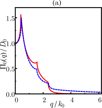
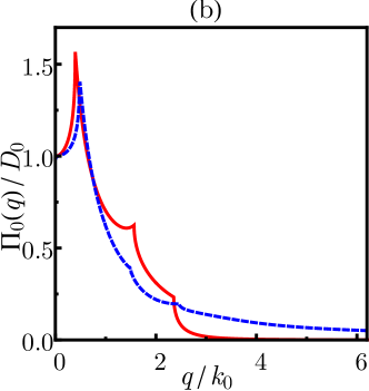
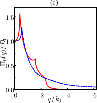
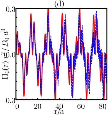
Figure 4: The static susceptibility from the full band dispersion (dashed blue line) and the approximate dispersion (solid red line) for (a) $\gamma_{1}=2\Delta$ (b) $\gamma_{1}=\Delta$ and (c) $\gamma_{1}=\Delta/2$, normalized to the density of states at the Fermi level, $D_{0}$.(d) Friedel oscillations in real space for $\gamma_{1}=2\Delta$ showing beating patterns. $\mu=0.15V_{dip}$ for all figures.

This analytic expression for susceptibility is also plotted in Fig.4 (a-c) with a solid red line. We see that the susceptibility matches well for small $q\sim\delta k$, but the weakening of the $2k_{\pm}$ singularities are not captured as the wavefunction overlaps are left out in this approximation.

The singularities of the susceptibility give rise to oscillations with corresponding wave-vectors in a)density patterns around defects (Friedel oscillation) and b) interaction between magnetic impurities (RKKY oscillations) RKKY . These oscillations can be experimentally verified by creating localized defects in the system. Since the oscillations asymptotically fall off as $1/r^{2}$, in Fig.4 (d), we plot $r^{2}\Pi^{0}(r)$ for $\gamma_{1}=2\Delta$ to illustrate the pattern of Friedel oscillations in the system, clearly showing the wave vectors involved.

The non-trivial Friedel oscillations can be used as an experimental signature of the presence of two Fermi surfaces in a system of non-interacting fermions. We next move on to the consequences of having two Fermi surfaces for a system of fermions interacting with repulsive Hubbard type interactions.

IV Stoner Instability and incommensurate SDW

We now consider a Bernal stacked bilayer honeycomb lattice of spin $1/2$ fermions which are interacting with a repulsive on-site interaction $U$. We note that we are considering a system of lattice fermions with repulsive interactions close to half filling; hence the cold atom system should be immune to the issues of atom loss which plague continuum systems in a trap without an optical lattice. The presence of the optical lattice reduces three body losses as long as the lattice is deep enough to consider only one band per degree of freedom. The presence of the lattice, however leads to Umklapp scattering and hence to 2 body atom loss in the system. This is clearly an experimentally accessible regime, since experiments with strong repulsive interactions in a lattice has already been performed showing the presence of Mott insulators Bloch_review . Typical experimentally measured timescales for atom loss, which can be achieved far from Feshbach resonances are $\sim 1-2$ sec. in these systems doublondecay . This relatively large timescale for atom loss ensures that the phenomena described in the following sections will not be washed out due to atom loss and should be easily accessible to experiments on this system.

IV.1 The Simple Stoner Picture

The low energy theory of biased Bernal-stacked bilayer consists of a sombrero like dispersion around the two inequivalent Dirac points, $\vec{K}$ and $\vec{K^{\prime}}$, which leads to a valley degree of freedom, $\tau$.

The local Hubbard interaction scatters fermions, both within a valley and between valleys, as seen in the Feynman vertices of Fig. 5(a) & (b). We assume that we are interested in momentum transfers q much smaller than $|\vec{K}-\vec{K}^{\prime}|$. Since we will later be concerned with incommensurate SDW states with $q\sim\delta k$, this is valid as long as $\delta k\ll|\vec{K}-\vec{K}^{\prime}|$. This implies that if a fermion is scattered from $\vec{K}$ to $\vec{K}^{\prime}$ valley, the other fermion must be scattered from $\vec{K}^{\prime}$ to $\vec{K}$ valley to conserve the total momentum. Consequently the $\tau$ indices of the Feynman vertex in Fig. 5(b) has more restrictions than those in Fig. 5(a).

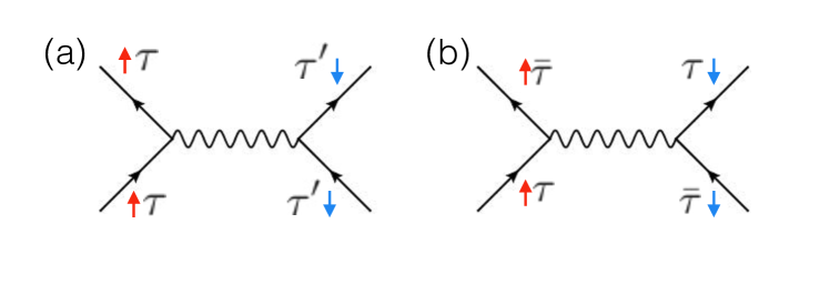
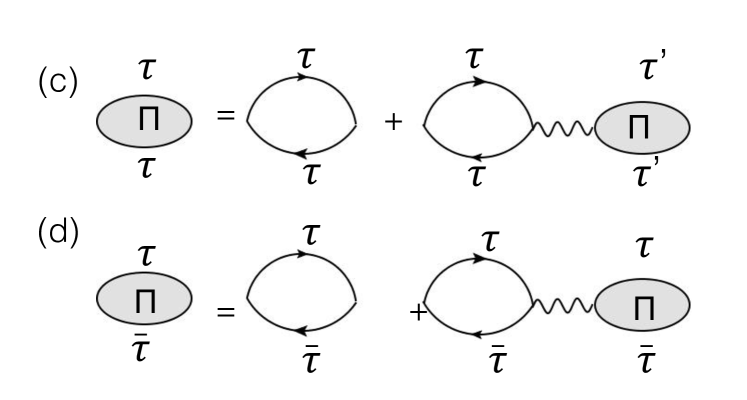
Figure 5: (a) and (b): Bare interaction vertices showing spin and valley indices of the participating fermions. (c) and (d): RPA diagrams for the dressed susceptibility for intravalley (c) and intervalley (d) terms

We use the notation $\Pi^{0}_{\tau\tau^{\prime}}(q)$ to define the intra-valley and inter-valley bare susceptibility with $\tau$ as the valley index ($\tau=\pm 1$ for $\vec{K}$ and $\vec{K^{\prime}}$). We note that $\Pi^{0}_{+-}(\vec{q})$ corresponds to a momentum transfer of $\vec{q}+\vec{K}-\vec{K^{\prime}}$. Within RPA approximation, we find that the intra-valley dressed susceptibility [Fig. 5 (c)] is given by

$$\Pi_{\tau\tau}(q)=\frac{\Pi^{0}_{\tau\tau}(q)}{1-U\sum_{\tau^{\prime}}\Pi^{0}_{\tau^{\prime}\tau^{\prime}}(q)}=\frac{\Pi^{0}_{\tau\tau}(q)}{1-2U\Pi^{0}_{\tau\tau}(q)}$$ (15)

We note that unlike the spin-independent Coulomb interactions, the local Hubbard interaction is only between fermions with opposite spins (see Fig. 5(a) and (b) ) and hence there is no spin sum for the intermediate bubbles in the RPA series. The spin states are fixed by the bare interaction vertex and we omit them here for the sake of brevity. For the dressed intra-valley susceptibility, the small momentum transfer implies all the intermediate bubbles are of the intra-valley type, but the fermions can be from either valley, resulting in the factor of $2$ in the denominator, as shown in Fig. 5(c). In contrast, the inter-valley dressed [Fig. 5(d)] susceptibility is given by

$$\Pi_{\tau\bar{\tau}}(q)=\frac{\Pi^{0}_{\tau\bar{\tau}}(q)}{1-U\Pi^{0}_{\bar{\tau}\tau}(q)}$$ (16)

where the restriction on $\tau$ indices of bare vertices in 5(b) implies that there is no valley summation to be done and therefore there is no factor of 2 in the denominator.

It is clear from the above argument that the intra-valley susceptibility undergoes a Stoner instability at a critical strength which is half that of the critical strength for the instability of the inter-valley susceptibility. Thus within the Stoner/RPA approximation, we can focus on the intra-valley susceptibility as the Stoner instability is dominated by the intravalley scattering, with the Stoner criterion Stoner

$$1-2U\Pi^{0}({\bf q},0)=0$$ (17)

where $2$ counts the valley degeneracy footnote3 . It is clear from Fig 4 that, as $U$ is increased, the first instability would occur at $q=\delta k$. From the analytic calculations, $\Pi^{0}(\delta k,0)=(\pi/2)\Pi^{0}(0,0)$, and so for $U>1/2\Pi^{0}(\delta k,0)$, the spin fluctuation modes at $q=k_{+}-k_{-}$ are most unstable, leading to an incommensurate spin-density wave order. As the chemical potential is lowered towards the van-Hove singularity at the band bottom, the critical repulsion for the instability, $U_{c}$, goes to zero $\sim\mu^{1/2}$. The critical coupling obtained from the simple Stoner criterion is plotted in Fig. 8 (a) and (b) for two different values of $\gamma_{1}/\Delta$, where the solid red curve corresponds to the result obtained from the approximate band calculation, while the blue dashed curve is obtained from the full band calculation. We note that the two results track each other closely, showing that the approximate band can be used to calculate the susceptibilities accurately in this regime. This will be crucial in the next section, where we will use the approximate band to include the effects of vertex corrections to the Stoner instability.

IV.2 Vertex Corrections and survival of Stoner Instability

Kanamori  Kanamori argued that since Stoner instability occurs at $U/W\sim 1$, where $W$ is the bandwidth of the system, one should consider the manybody renormalization of the interaction which can be strong enough to prevent the Stoner instability. In this case, the instability occurs at weak couplings as we move towards the band bottom, and survives the logarithmic reduction of the repulsive interaction. To show this, we consider the vertex corrections to the spin susceptibility within the analytic one-band model given by Pekker

$$\Pi_{\tau\tau}(q) = \sum_{k}G_{\tau}(k)G_{\tau^{\prime}}(k+q)\Lambda_{\tau\tau^{\prime}}(k,q)$$ (18)

where $k$ denotes both a momentum sum and a Matsubara frequency sum, and the greens function is $G(k)=G(\vec{k},\omega)=(\omega-\epsilon_{k}+\mu)^{-1}$. The Bethe-Salpeter type equation for the vertex function can be obtained from diagrammatic resummation [Feynman diagrams in Fig .6(a)],

$$\Lambda_{\tau\tau}(k,q) = 1+\sum_{k^{\prime},\tau^{\prime}}\Gamma^{\tau\tau^{\prime}}_{\tau\tau^{\prime}}(k,k^{\prime},q)G_{\tau^{\prime}}(k^{\prime})G_{\tau^{\prime}}(k^{\prime}+q)\Lambda_{\tau^{\prime}\tau^{\prime}}(k^{\prime},q)~{}~{}~{}\text{and}$$

$$\Lambda_{\tau\bar{\tau}}(k,q) = 1+\sum_{k^{\prime}}\Gamma^{\tau\bar{\tau}}_{\bar{\tau}\tau}(k,k^{\prime},q)G_{\bar{\tau}}(k^{\prime})G_{\tau}(k^{\prime}+q)\Lambda_{\tau\bar{\tau}}(k^{\prime},q)$$ (19)

where we have assumed $\Lambda_{\tau\bar{\tau}}=\Lambda_{\bar{\tau}\tau}$.The full four-point interaction vertex is approximated by the ladder sum leading to the T matrix renormalization of the interaction strength.[Feynman diagram in Fig .6(b)]

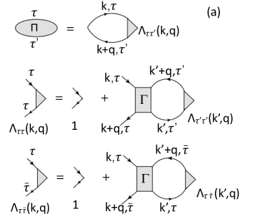
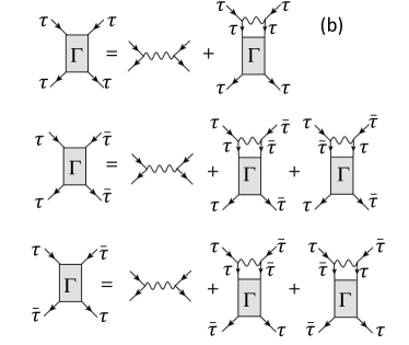
Figure 6: (a) Feynman diagrams corresponding to vertex correction to susceptibility, $\Lambda$ and the integral equations for $\Lambda$ from the partial resummation of the series. (b) The Feynman diagrams corresponding to ladder resummation of the four-point vertex (effective interaction). The $\tau=\pm 1$ indices correspond to the valleys $K$ and $K^{\prime}$

$$\Gamma^{\tau\tau}_{\tau\tau}(k,k^{\prime},q) = U-U\sum_{k_{1}}G_{\tau}(k_{1})G_{\tau}(-k_{1}+q)\Gamma^{\tau\tau}_{\tau\tau}(k_{1},k^{\prime},q)$$ (20)

$$\Gamma^{\tau\bar{\tau}}_{\tau\bar{\tau}}(k,k^{\prime},q) = U-U\sum_{k_{1}}[G_{\tau}(k_{1})G_{\bar{\tau}}(-k_{1}+q)\Gamma^{\tau\bar{\tau}}_{\tau\bar{\tau}}(k_{1},k^{\prime},q)+G_{\bar{\tau}}(k_{1})G_{\tau}(-k_{1}+q)\Gamma^{\bar{\tau}\tau}_{\tau\bar{\tau}}(k_{1},k^{\prime},q)]~{}~{}~{}and$$

$$\Gamma^{\tau\bar{\tau}}_{\bar{\tau}\tau}(k,k^{\prime},q) = U-U\sum_{k_{1}}[G_{\tau}(k_{1})G_{\bar{\tau}}(-k_{1}+q)\Gamma^{\tau\bar{\tau}}_{\bar{\tau}\tau}(k_{1},k^{\prime},q)+G_{\bar{\tau}}(k_{1})G_{\tau}(-k_{1}+q)\Gamma^{\bar{\tau}\tau}_{\bar{\tau}\tau}(k_{1},k^{\prime},q)]$$

Since the Greens functions do not depend on $\tau$, we see that $\Lambda_{\tau\tau}$ and $\Lambda_{\tau\bar{\tau}}$ are independent of the index $\tau$ and hence obtain the T matrix renormalization of the interaction vertex

$$\Gamma^{\tau\tau}_{\tau\tau}(q)=\left[\frac{1}{U}-C(q)\right]^{-1}~{}~{}~{}~{}~{}~{}~{}~{}\Gamma^{\tau\bar{\tau}}_{\tau\bar{\tau}}(q)=\left[\frac{1}{U}-2C(q)\right]^{-1}~{}~{}~{}and~{}~{}~{}~{}~{}~{}~{}\Gamma^{\tau\bar{\tau}}_{\bar{\tau}\tau}(q)=\left[\frac{1}{U}-2C(q)\right]^{-1}$$ (21)

where $C(q)=-\sum_{k}G(k)G(-k+q)$ is the non-interacting Cooperon propagator. Once again it is clear that the intravalley susceptibility has stronger instabilities. Focussing on the intravalley susceptibility, and dropping the $\tau$ indices, we get

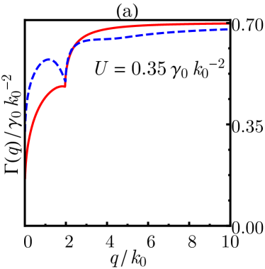
Figure 7: (a) The renormalized interaction $\Gamma(q)$ as a function of $q$ for $U=U_{c}=0.32\gamma_{0}$ for the approximate one band (red solid line) and the full band (blue dashed line). (b)The comparison of $U_{c}$ obtained by setting $Det[1-B]=0$ (blue solid line) and by setting $1-B_{00}=0$ (red dashed line). The two methods give comparable results. Both (a) and (b) are obtained for $\gamma_{0}=\gamma_{1}=\Delta$ and $\mu=0.15V_{dip}$.

$$\Pi(q) = \sum_{k}G(k)G(k+q)\Lambda(k,q)$$ (22)

$$\Lambda(k,q) = 1+\sum_{k^{\prime}}\Gamma(k+k^{\prime}+q)G(k^{\prime})G(k^{\prime}+q)\Lambda(k^{\prime},q)$$

$$\Gamma(q) = \left[\frac{1}{U}-C(q)\right]^{-1}+\left[\frac{1}{U}-2C(q)\right]^{-1}$$

Within the one band model, the Cooperon propagator is given by

$$C(q)=\sum_{k}\frac{1-n_{F}(\xi_{k})-n_{F}(\xi_{k+q})}{\omega-\xi_{k}-\xi_{k+q}}$$ (23)

We note that for the approximate band, we can take the momentum cutoff to $\infty$ without any ultraviolet divergence, as the large $k$ dispersion $\sim k^{4}$ in this case. The linear dispersion at large $k$ for the full band requires a cutoff of $\sim 1/a$, while including the complete dispersion for the hexagonal lattice cuts off the linear dispersion and gives a finite answer. We have checked by explicit enumeration that in the range of $q$ that we are interested in, the choice of different cutoffs do not affect our answers. A plot of $\Gamma(q)$ as a function of $q$ for both the one-band and full-band model with $\gamma_{0}=\gamma_{1}=\Delta$ and $\mu=0.15V_{dip}$ at $U=U_{c}\sim 0.32\gamma_{0}/k_{0}^{2}$, is shown in Fig 7(a). The effective interaction increases with $q$ and the bare answer $2U$, with $2$ for valley degeneracy factor, is recovered in the large $q$ limit.

The divergence of the susceptibility is governed by a divergence of the vertex factor $\Lambda$ Pekker , which is controlled by contributions from the momentum space where the two poles of the Green’s functions $G(k)$ and $G(k+q)$ come close to each other. For the static susceptibility (zero external frequency), the main contribution comes when $\vec{k}$ and $\vec{k^{\prime}}$ both lie on a Fermi surface. There are two possibilities: $|\vec{k}|$ and $|\vec{k^{\prime}}|$ can lie on either of the two Fermi wave-vectors $k_{+}$ and $k_{-}$. We also set $|\vec{q}|=\delta k$, the thickness of the Fermi sea, where the strongest instability is seen in the RPA approximation. We have checked by varying $|\vec{q}|$ that this choice corresponds to the strongest instability. We also find that the choice $|\vec{k}|=|\vec{k^{\prime}}|=k_{+}$ corresponds to the strongest instability. This can be seen from the fact that the effective interaction $\Gamma(q)$ increases with $q$, i.e. the renormalization becomes less effective with increasing $q$.

So, we fix the value of $|\vec{k}|$ and $|\vec{k^{\prime}}|$ in all the terms of the integral equation for $\Lambda$, except the product of the Green’s functions, which are rapidly varying function of the radial co-ordinates Pekker . The integral equation for $\Lambda$ then reduces to

$$\Lambda(\hat{k},\vec{q})=1+\int d\hat{k^{\prime}}\Gamma(k_{+}(\hat{k}+\hat{k^{\prime}})+\vec{q})\Lambda(\hat{k^{\prime}},\vec{q})I(\hat{k^{\prime}},\vec{q})$$ (24)

where

$$I(\hat{k^{\prime}},\vec{q}) = \frac{1}{4\pi^{2}}\int k^{\prime}dk^{\prime}G(k^{\prime})G(k^{\prime}+q)$$ (25)

Without loss of generality, we assume that $\vec{q}$ lies along the $x$ axis. The integral equation is then a function of two angles, $\theta$ corresponding to $\hat{k}$ and $\theta^{\prime}$ corresponding to $\hat{k^{\prime}}$. Expanding $\Lambda(\theta)=\frac{1}{2\pi}\sum_{m}\Lambda_{m}e^{im\theta}$, and constructing the vector $\hat{\Lambda}$ of the fourier components, we can then write a matrix equation

$$\hat{\Lambda}=(1-B)^{-1}\hat{w}$$ (26)

where $\hat{w}_{m}=\delta_{m0}$ and

$$B_{mn}=\frac{1}{2\pi}\int_{0}^{2\pi}d\theta^{\prime}\Gamma(\theta,\theta^{\prime})I(\theta^{\prime})e^{in\theta^{\prime}-im\theta}$$ (27)

The instability criterion is then given by

$$Det(1-B)=0$$ (28)

However a simpler criterion $1-B_{00}=0$ gives an $U_{c}$ which is remarkably close to the full answer [Fig. 7(b)], which shows that the instability is essentially driven by the $m=0$ mode. We find that increasing the size of the matrix $B$ does not lead to appreciable changes, thus confirming that higher $m$ modes do not contribute to the instability.

The critical coupling $U_{c}$ as a function of $\mu$ in this vertex corrected scenario is shown in Figs. 8 (a) and (b) (black triangles). We find that the critical coupling increases from the simple Stoner prediction, but the vertex corrected values can be easily accessed experimentally in cold atom systems. We also see that the vertex corrected critical coupling still decreases to zero as the density is decreased towards half-filling and the instability is robust with respect to vertex renormalizations.

We can also estimate the time-scale for formation of the ferromagnetic domains by considering the location of the pole of the susceptibility on the positive imaginary axis of the complex frequency plane when interactions are tuned beyond the instability. We find this time-scale for the growth of the domains to be $\sim 10^{-5}s$, which is much shorter than the atom loss time scale $\sim 1s$ doublondecay in these systems. Thus this instability should be clearly visible in the experiments.

Thus the Stoner instability is robust to the vertex corrections. In the next section, we will see that the ladder diagrams represent the most important corrections to the interaction vertex in a perturbative renormalization group procedure, and thus we have shown that the Stoner instability is robust to such corrections.

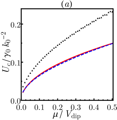
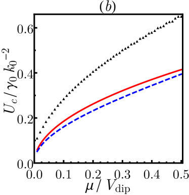
Figure 8: (a) $U_{c}$ as function of $\mu$ within Stoner calculation with approximate band (solid red line), full band (dashed blue line) and the result of including vertex corrections (black triangles) for $\gamma_{0}=\Delta$ and (a) $\gamma_{1}=2\Delta$ and (b) $\gamma_{1}=\Delta$.

IV.3 Stability of the Incommensurate SDW state

It is well known BelitzRMP ; Vojta1 ; Simmons ; Conduit that the presence of gapless fermionic particle-hole excitations and the coupling of the order parameter to these soft modes leads to a first order phase transition in the case of a Stoner transition to a usual ferromagnetic state with a $q=0$ order parameter. In certain parameter regimes, this first order transition is pre-empted by a continuous transition to a spin-spiral state with a broken translational symmetry Vojta1 . In this section, we consider the soft fermionic modes that our incommensurate SDW order parameter couples to and show that they do not lead to a pre-emption of the Stoner transition in this case of a finite $q=\delta k$ order parameter.

In case of the uniform ferromagnetic order, the order parameter couples to particle-hole excitations at small wavevectors $q\rightarrow 0$ and low frequencies $\omega\rightarrow 0$. The density of states of these excitations have a singular behaviour in this case $\sim\omega/q$, which invalidates the usual Landau Ginzburg expansion around a continuous transition and leads to a first order transition. In our case, the low energy theory is dominated by the coupling of the order parameter $\vec{m}_{q}$ to the soft fermionic modes at $q\rightarrow\delta k$ and $\omega\rightarrow 0$ through a term in the action

$$S\sim g\int d\tau m^{+}_{q}(\tau)\sum_{k}\psi^{\dagger}_{\downarrow k}(\tau)\psi_{\uparrow k+q}(\tau)+h.c.$$ (29)

where, for the sake of concreteness, we are considering the order-parameter to lie in the $x-y$ plane, $\psi_{\sigma k}$ is the fermion annihilation operator with spin $\sigma$ and momentum $k$ and $g$ is a coupling parameter. The density of these excitations can be obtained from the imaginary part of the momentum and frequency dependent retarded polarization function $\Pi(q,\omega+i0^{+})$ in this system. We use the one band model with the quartic dispersion, $\epsilon_{k}=\epsilon_{0}(k^{2}-k_{0}^{2})^{2}$, which was used in the previous section to compute this function and get

$$\Pi(q,\omega)=-\frac{1}{2\pi^{2}}\int_{k_{-}}^{k_{+}}kdk\int_{0}^{\pi}d\phi\left[\frac{1}{\omega+i0^{+}-\epsilon_{0}\alpha(2k^{2}+\alpha-k_{0}^{2})}-\frac{1}{\omega+i0^{+}-\epsilon_{0}\beta(2k^{2}-\beta-k_{0}^{2})}\right]$$ (30)

where $\alpha=2kq\cos\phi+q^{2}$ and $\beta=2kq\cos\phi-q^{2}$.

We have explicitly calculated the full frequency and momentum dependent polarization function near $q=\delta k$ and $\omega=0$ and find (both numerically and analytically) that the real part $\Pi^{{}^{\prime}}\sim const+\sqrt{|q-\delta k|}$ whereas $\Pi^{{}^{\prime\prime}}\sim\omega$. We note that unlike the case of usual uniform ($q=0$) order parameter, the density of excitations does not have any non-analyticity. Furthermore the finite $q$ order parameter couples in an off-diagonal channel and hence the incommensurate density wave is not unstable to the soft fermionic modes. We note that we are considering a region in phase space, where there is no instability towards uniform magnetism and the fluctuations of the uniform order parameter is gapped on a sufficiently large scale (in fact this scale can be made as large as possible by going closer to the Van-Hove singularity). Thus, unlike the uniform magnetic order, the incommensurate SDW does not lead to a first order transition. Furthermore, since there is no instability toward uniform order, there is no chance of obtaining a spin-spiral where a transverse propagating spin mode is superimposed on a uniform background. The incommensurate SDW, of course leads to spatial oscillation of the order-parameter in the system. Finally, we have not seen any evidence of formation of nematic ordered states, although such quadrupolar ordering cannot be ruled out completely. In the next section, we construct an RG flow, which does not show any tendency towards Pomeranchuk instabilities, although a truly spontaneously broken nematic order is beyond the purview of such calculations.

V Renormalization Group and Competing Orders

In the previous sections, we have shown that the system with two Fermi surfaces possess a Stoner-like instability towards an incommensurate spin-density-wave order and this instability is robust to incorporating particle-particle correlations through vertex corrections. Since Stoner instability is a threshold phenomenon, i.e. it requires a finite coupling before the instability occurs, it is legitimate to ask whether this is pre-empted by an instability at infinitesimal coupling towards a competing order like charge density wave or superconductivity. Such perturbative instabilities, if they are present, would drive the system towards these alternate symmetry broken states. The formalism which treats competing orders on an equal footing is renormalization group analysis, and it can pick out relevant orders and the relative strength of instabilities in an unbiased way.

In the case of fermions with one Fermi surface, it is known ShankarRG that in dimensions more than one, the only relevant instability is the superconducting instability with infinitesimal attractive interactions, unless the Fermi surface is nested Honerkamp ; MetznerRMP , when density wave instabilities can occur. The case of fermions with two Fermi surfaces Nk1 ; Nk2 , well separated in momentum space has been worked out in the context of pnictide superconductors pnictide ; Chubukov1 ; Chubukov2 , where a competition between a spin-density-wave order and superconductivity is seen. In that case, the presence of a hole pocket and an electron pocket, with Fermi velocities of opposite signs, lead to one loop renormalization of both the interaction vertex which drives SDW and the vertex which drives superconductivity and depending on the details of the system, different orders can prevail in the system.

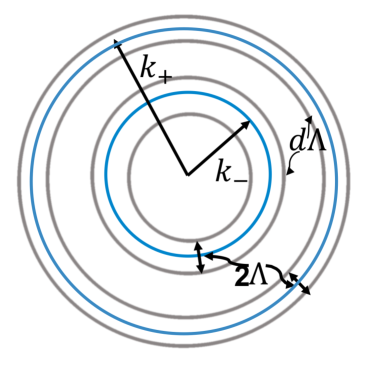
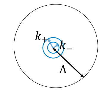
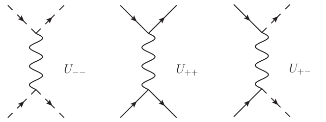
Figure 9: Schematic sketch of cutoffs and momentum shells being integrated out in RG when (a) $\Lambda<\delta k/2$ and (b) $\Lambda\gg k_{\pm}$. (c) The Feynman vertices for the bare couplings showing intra and inter Fermi surface scatterings.

We would first like to point out that the geometry of our two fermi surfaces is quite different from that found in pnictides, which has two small Fermi surfaces separated by a large momentum in the Brillouin zone. In our case, we have an annular Fermi sea with two concentric circles as the Fermi surfaces. Let us first consider a cutoff scale $\Lambda\gg k_{0},\Lambda\gg k_{\pm}$. In this case, it is impossible to unambiguously define electrons around the two Fermi surfaces, and for all practical purposes, the system behaves as if it had one Fermi surface. This situation is shown in Fig. 9 (b). In this case, the standard RG of Fermions with a single Fermi surface ShankarRG holds and both the forward scattering amplitude and the interaction in the particle-particle channel are marginal at tree level and, for repulsive interactions, renormalizes down logarithmically. This logarithmic reduction is precisely what is captured by the ladder type vertex corrections shown in the previous section. This does not lead to any perturbative instabilities by itself, while the Stoner instability has been shown to be robust to these corrections. The key reason for this is that while the reduction due to RG is logarithmic, the threshold required to attain the Stoner instability decreases as the square root of the energy scale (Fermi energy) and hence prevails over the logarithmic reduction.

A clear distinction between the two Fermi surfaces can be made when $\Lambda<\delta k/2$, when one can unambiguously talk about low energy fermions around the two Fermi surfaces, as shown in Fig. 9(a). In this case, the renormalization group calculation proceeds along the lines of Ref. Chubukov1 . The key interaction vertices in the different channels are shown in Fig. 9(c). Here $U_{++}$ represents a process where two fermions with total momentum $0$ and lying near the Fermi surface $+$ are scattered two other states near $+$ with zero net momentum. $U_{--}$ is the same process with all the fermions near the $-$ Fermi surface and $U_{+-}$ is the process where a total zero momentum pair is scattered from $+$ to $-$ Fermi surface. In addition there are forward scattering processes which are not shown as they are not renormalized in one loop RG. In principle the particle-hole diagrams can also pick up a logarithmic divergence due to the change in the sign of the Fermi velocity between the Fermi surfaces. However, a key difference from the RG flows for pnictides is that in this case, since the Fermi surfaces are concentric, these couplings do not flow under one loop RG due to phase space restrictions, coming from constraints of momentum conservation around the Fermi surfaces. The RG flow for the intra and inter Fermi surface BCS type dimensionless couplings $U_{++}$, $U_{--}$ and $U_{+-}=U_{-+}$ are given by

$$\frac{d\hat{U}}{dl}=-\hat{U}^{2}$$ (31)

where $\hat{U}$ is a $2\times 2$ matrix $\left(\begin{array}[]{cc}U_{++}&U_{+-}\\ U_{-+}&U_{--}\end{array}\right)$ and $dl=d\Lambda/\Lambda$. The Feynman diagrams corresponding to this flow equation are shown in Fig. 10(a). We would like to note that the Fermi velocities at the 2 Fermi surfaces are not equal ($v_{+}\neq v_{-}$), but the factor of $v_{+}$ or $v_{-}$ drops out when the couplings are made dimensionless using the density of states at the respective Fermi surfaces, $N_{0}=(1/2\pi)k_{+}/v_{+}=(1/2\pi)k_{-}/v_{-}$. These equations can be solved analytically to obtain the flow diagram of the couplings. The equations are most easily solved by variable transform to $\phi=2U_{+-}/(U_{++}-U_{--})$, $v=(U_{++}+U_{--})/2$ and $r=\sqrt{U^{2}_{+-}+(U_{++}-U_{--})^{2}/4}$. It can be easily shown that $\phi$ does not flow under RG, while the flow patterns in the $v-r$ plane is shown in Fig. 10(b).

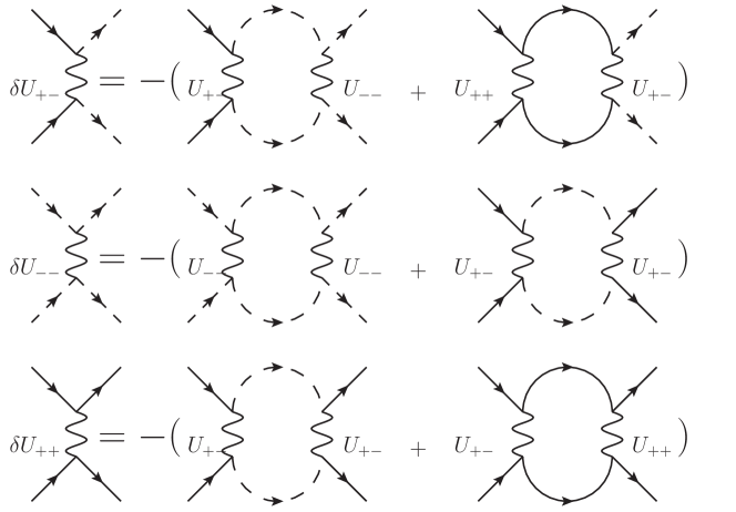
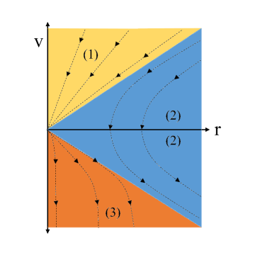
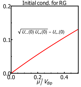
Figure 10: (a) Feynman diagrams corresponding to one loop correction of the interaction vertices. (b) The RG flow diagram showing regions where the Fermi liquid is stable and regions where a superconducting instability takes over. (c) Calculated initial conditions showing that the system lies in the stable region and hence does not show a perturbative superconducting instability. Thus the Stoner threshold behaviour is not destroyed by any competing perturbative instability.

The half-plane is divided into three distinct regions by the lines $v=r$ and $v=-r$. For $v>0$, if $v>r$ (yellow region (I)), the interaction parameters are all renormalized to zero under RG and the Fermi liquid does not have any perturbative instabilities. For $v<0$, $v<r$ (orange region (III)), the flow moves away from the Fermi liquid fixed point at the origin. This corresponds to standard attractive superconducting instabilities, and since $|v|>r$, the pairing will be dominated by the intra Fermi surface pairing. In the blue region (II), $|v|<r$. If the flow starts from $v>0$, the interaction scales are initially renormalized downwards, before growing in the negative direction with $v=-r$ and $r\rightarrow\infty$. This flow needs to be cutoff when $r\sim 1$ to obtain critical points. We note that this case corresponds to the $s^{\pm}$ superconducting pairing instability, where the pairing symmetry is $s-wave$ on both Fermi surfaces, but the pairing function changes sign between the Fermi surfaces. Thus, we find that the only perturbative instability in the system is towards superconductivity, provided the flow starts from either the blue or the orange regions in the phase diagram shown in Fig. 9 (b). We note that there is no instability towards triplet superconductivity within this RG.

It is then important to determine where our system lies in this phase diagram. The system will have a perturbative superconducting instability provided $|v|<r$, i.e. $U_{+-}<\sqrt{|U_{++}U_{--}|}$. We first estimate the interactions at the microscopic scale. The microscopic values of the intra and inter Fermi surface couplings, obtained from the Hubbard U and the band wavefunctions, are shown in section  II. To calculate this, it is useful to work in the momentum space

$$H_{\text{int}}=U\sum_{\tau,k,k^{\prime},q}c^{\dagger}_{\tau}(k)c_{\tau}(k+q)c^{\dagger}_{\tau}(k^{\prime})c_{\tau}(k^{\prime}-q)$$ (32)

. Here $\tau$ is the layer/sublattice index and from (5) $c^{\dagger}_{\tau}(k)=\phi^{-}_{+}(k)_{[\tau]}a^{\dagger}(k)$, where $a_{k}$ is the low energy electron operator in the band basis (we consider only the band where the chemical potential lies). Projecting onto the band basis and working with momenta on the respective Fermi surfaces, one can easily construct $U_{++}$, $U_{--}$ and $U_{+-}$ for the system. We find that the system is always in the regime where the Fermi liquid is stable to perturbative instabilities. In Fig 10(c), we plot $\sqrt{|U_{++}U_{--}|}-U_{+-}$ as a function of the chemical potential and show that this is always positive. This remains true under the weak logarithmic reduction from the RG with large cutoff (which is similar to RG with one Fermi surface), and thus the Stoner instability is not overtaken by any other perturbative instabilities. We note that the Stoner instability remains a threshold phenomenon, i.e. a finite coupling strength is required to reach this instability, and is not captured by the perturbative RG that we have constructed. We would also like to note that there is an intermediate scale from $\Lambda\sim k_{\pm}$ to $\Lambda\sim\delta k/2$, where the RG procedure cannot be carried out since the non-linearities of the dispersions do not allow a reasonable scaling analysis to start the procedure.

We would also like to note that if we start from the insulating phase, i.e. at the band-bottom, the effective dispersion $\sim k^{2}$, and this would lead to non-Fermi liquid behaviour. However, chemical potential is a relevant potential at this non-Fermi liquid fixed point and the system flows to a Fermi liquid at any finite chemical potential, which then undergoes the Stoner instability described in the previous sections. This also clearly shows that the finite chemical potential should be described in terms of an itinerant system and its instabilities rather than as an insulating system.

Finally, having dispelled off the possibility of perturbative instabilities, we have also checked that competing orders like charge density wave, spin spirals and superconductivity of different orbital symmetry do not win over the incommensurate spin-density wave instability in the system. We have also checked for the possibility of Pomeranchuk type instabilities and have not found any of the Pomeranchuk channels to be more unstable than the SDW instability. We note that we have only checked for order parameters which are bilinear in the fermion fields, which leaves open the possibility of a nematic order, which is impossible to pick up in a one loop perturbative RG calculation. However, the nematic order, which involves breaking down the $C_{6}$ symmetry of the lattice to a $C_{2}$ symmetry, would require the inter-valley and intra-valley effective interactions to be comparable. We have earlier shown, both within RPA and with inclusion of vertex corrections, that the inter-valley effective interactions are better screened and hence much weaker than intra-valley effective interactions. Thus a nematic instability is unlikely to occur in the case where the finite density of states leads to differential screening of the intra-valley and inter-valley interactions. In fact, if lattice effects (trigonal distortions) are included, the main effect of the imposition of discrete lattice symmetry is that the SDW wave-vector will lose the rotational symmetry and would choose between three degenerate vectors dictated by the effective $C_{3}$ symmetry around each Dirac valley.

VI Conclusion and Discussions

Itinerant fermions with multiple Fermi surfaces can lead to interesting phenomenology in a many body system. The biased Bernal stacked bilayer honeycomb lattice provides such a system at densities close to half-filling, with an annular Fermi sea. In this paper, we have proposed a simple scheme of implementing a Bernal-stacked bilayer lattice with ultracold atoms, which is a modification of schemes already used by experimentalists to implement a planar honeycomb lattice. The low energy band dispersion in this system has the shape of a sombrero and results in an annular Fermi sea with concentric Fermi surfaces at low densities. We have used band structure calculations to correlate the optical lattice parameters to the tight binding parameters of the problem. We have shown that there is a wide range of experimentally accessible parameters, where the effects of the annular Fermi sea can be clearly seen.

The sombrero like dispersion at low densities, and the consequent presence of two Fermi wave-vectors in the system leads to singularities in the static polarizability function of the system, which controls the response of the system to potential perturbations. We find that naive phase space arguments would predict $4$ singularities, whereas $3$ are actually seen in the calculations. The absence of the fourth singularity at a wave-vector equal to the sum of the two Fermi wave vectors can be explained through a subtle cancellation of contribution from two Fermi surfaces. The singularities in the static polarizability is reflected in the occurrence of Friedel and RKKY oscillations with three wave-vectors, which can be seen experimentally, thus providing an evidence of the presence of multiple Fermi wave-vectors.

If the fermions placed in this lattice are interacting with a Hubbard repulsion, there is a quantum phase transition to an incommensurate spin density wave state with a wave-vector equal to the thickness of the Fermi sea. Within a simple Stoner approximation, the critical coupling for this transition goes to zero as the density of the system is lowered and the chemical potential approaches the Van Hove singularity at the band bottom. The inclusion of vertex corrections, which are the leading order correction from a renormalization group analysis at large cutoff, does not change this picture substantially, with small quantitative changes in $U_{c}$. The Stoner instability is thus robust to many body renormalization of the couplings between fermions. We note that by virtue of the azimuthal symmetry of our low energy model, the modulus of the incommensurate wave-vector is specified while its direction is indeterminate within our calculation. In reality, we have neglected small lattice effects like trigonal warping, which will break the circular symmetry, and choose a direction with a three-fold degeneracy respecting the lattice symmetry of the full model.

We also construct a perturbative renormalization group flow for this system to treat competing order parameters on an equivalent footing. We show that the large cutoff RG leads to a logarithmic reduction of the interaction strength, well understood in the RG of fermions with a single Fermi surface. This is in contrast with RG flow for two Fermi surface systems like iron pnictides, where the RG flow leads to increasing couplings and a non-trivial fixed point. The main reason our RG flow follows that of a single Fermi surface is that unlike pnictides, which have small Fermi seas separated by a large almost commensurate wave-vector, our Fermi surfaces are concentric, and at large cutoff, the system behaves as if there is only one Fermi surface. At small cutoffs, where the two Fermi surfaces can be clearly distinguished, there is a superconducting instability in parts of the parameter regime, but we show that our system falls outside this parameter regime, and hence there are no perturbative instabilities. Thus in absence of perturbative instabilities, the Stoner instability towards SDW states prevail over other instabilities to remain the dominant threshold instability. We note that we have considered competing orders which are bilinear in the fermion fields, and a nematic instability remains a possibility, which we cannot probe with our approach. We would also like to note that while our RG procedure is well defined for very large and very small cutoffs, there is a range of scales from $k_{+}$ to $\delta k$, where it is not possible to do a reliable RG calculation. Within these caveats, we find the Stoner instability towards the incommensurate spin-density-wave state to be the dominant instability of the system.

The predicted incommensurate spin density wave order can be identified by different experimental techniques. Noise measurements noise and spectroscopic techniques like spin-dependent Bragg spectroscopy bragg and optical lattice modulation spectroscopy optlat can be used to look at the finite wave vector spin order. Alternatively, a quantum quench across the critical coupling would lead to the growth of magnetic domains Pekker with a length scale which corresponds to the most unstable mode. In this case, the growth of the most unstable mode at $q=\delta k$ can be observed using real space imaging techniques.

VII Acknowledgments

R. S. wishes to thank Sankar Das Sarma, David Pekker and Kazi Rajibul Islam for useful discussions. S. D. wishes to thank Tomi H. Johnson for help with the MLGWS software package. R.S. and S.D acknowledge computational facilities at the Dept. of Theoretical Physics, TIFR Mumbai.

References

- (1) B. J. Lawson, Paul Corbae, Gang Li, Fan Yu, Tomoya Asaba, Colin Tinsman, Y. Qiu, J. E. Medvedeva, Y. S. Hor, and Lu Li, Phys. Rev. B 94, 041114(R) (2016).
- (2) L. Taillefer and G. G. Lonzarich, Phys. Rev. Lett. 60, 1570 (1988).
- (3) K. Kuroki, S. Onari, R. Arita, H. Usui, Y. Tanaka, H. Kontani, and H. Aoki, Phys. Rev. Lett. 101, 087004 (2008).
- (4) G. R. Stewart, Rev. Mod. Phys. 83, 1589 (2011)
- (5) S. Mozorov et al., Phys. Rev. Lett. 100, 016602 (2008); K. Novoselov et al., Nature Phys. 2, 177 (2006).
- (6) E. McCann and V. I. Falko, Phys. Rev. Lett. 96, 086805 (2006); J. Nilsson, A. H. Castro Neto, N. M. R. Peres and F. Guinea, Phys. Rev. B 73, 214418 (2006); A. H. Castro Neto et. al, Rev. Mod. Phys. 81, 109 (2009).
- (7) O. Vafek and K. Yang, Phys. Rev. B 81, 041401(R) (2010);V. Cvetkovic, R. E. Throckmorton, and O. Vafek Phys. Rev. B 86, 075467 (2012).
- (8) F. Zhang, H. Min, and A. H. MacDonald, Phys. Rev. B 86, 155128 (2012); J. Velasco Jr, Y. Lee, F. Zhang, K. Myhro, D. Tran, M. Deo, D. Smirnov, A. H. MacDonald and C. N. Lau, Nat. Comm. 5, 1 (2014).
- (9) Y. Barlas and K. Yang, Phys. Rev. B 80,161408(R) (2009); R. Nandkishore and L. Levitov, Phys. Rev. B 82, 115431 (2010).
- (10) R. Sensarma, E. H. Hwang and S. Das Sarma, Phys. Rev. B 84, 041408(R) (2011).
- (11) S. Das Sarma, E. H. Hwang, E. Rossi Phys. Rev. B 81, 161407 (2010); E. Rossi, S. Das Sarma Phys. Rev. Lett. 107, 155502 (2011)
- (12) J. B. Oostinga, H. B. Heersche, X. Liu, A. F. Morpurgo and L. M. K. Vandersypen, Nature Mat. 7, 151 (2007). E. V. Castro, K. S. Novoselov, S. V. Morozov, N. M. R. Peres, J. M. B. Lopes dos Santos, J. Nilsson, F. Guinea, A. K. Geim, and A. H. Castro Neto, Phys. Rev. Lett. 99, 216802 (2007).
- (13) L. Ju, Z. Shi, N. Nair, Y. Lv, C. Jin, J. V. Jr, C. Ojeda-Aristizabal, H. A. Bechtel, M. C. Martin, A. Zettl, J. Analytis, F. Wang, Nature 520, 650-655 (2015)
- (14) I. Bloch, J. Dalibard and W. Zwerger, Rev. Mod. Phys. 80, 885 (2008).
- (15) C. Guerlin, K. Baumann, F. Brennecke, D. Greif, R. Joerdens, S. Leinss, N. Strohmaier, L. Tarruell, T. Uehlinger, H. Moritz, and T. Esslinger, in Laster Spectroscopy, ed. by H. Katori, H. Yoneda, K. Nakagawa, and F. Shimizu, Vol. 1 (World Scientific, Singapore, 2010), p. 212.
- (16) M. Greiner, et al., Nature 415, 39 (2002); C. Orzel et al., Science 291, 2386 (2001).
- (17) E. V. Castro, N. M. R. Peres, T. Stauber, N. A. P. Silva, Phys. Rev. Lett. 100, 186803 (2008).
- (18) L. M. Duan, E. Demler and M. Lukin, Phys. Rev. Lett. 91, 90402 (2003).
- (19) L. Tarruell, D. Greif, T. Uehlinger, G. Jotzu and T. Esslinger, Nature 483, 302 (2012); G. Jotzu, M. Messer, R. Desbuquois, M. Lebrat, T. Uehlinger, D. Greif and T. Esslinger, Nature 515, 237 (2014); L. Duca, T. Li, M. Reitter, I. Bloch, M. Schleier-Smith and U. Schneider, Science 347, 288 (2015).
- (20) Hong-Shuai Tao, Yao-Hua Chen, Heng-Fu Lin, Hai-Di Liu, Wu-Ming Liu, Sci. Rep. 4, 5367 (2014).
- (21) E. McCann and V. I. Falko, Phys. Rev. Lett. 97, 146805 (2006).
- (22) In addition, there is a weak tunneling between and , and between . In this paper we have set these weak tunneling parameters to .
- (23) K. L. Lee, B. Grémaud, R. Han, B-G Englert, and C, Miniatura, Phys. Rev. A 80, 043411 (2009).
- (24) J. Ibanez-Azpiroz, A. Eiguren, A. Bergara, G. Pettini, and M. Modugno, Phys. Rev. A 87, 011602(R) (2013).
- (25) There is a factor of 2 difference in the definition of the lattice potential between our convention and that of Ref. coldatom_bandparam_2 .
- (26) The tight binding parameter was obtained by using the MLGWS package (https://ccpforge.cse.rl.ac.uk/gf/project/mlgws/), which is based on R. Walters, G. Cotugno, T. H. Johnson, S. R. Clark, and D. Jaksch, Phys. Rev. A 87, 043613 (2013); I Souza, N. Marzari and D. Vanderbilt, Phys. Rev. B 65, 035109 (2001); N. Marzari and D. Vanderbilt, Phys. Rev. B 56, 12847 (1997).
- (27) E. McCann and V. I. Falko, Rep. Prog. Phys. 76, 056503 (2013).
- (28) E. H. Hwang and S. Das Sarma, Phys. Rev. Lett. 101, 156802 (2008).
- (29) N. W. Ashcroft and N. D. Mermin, Solid State Physics, Harcourt College Publishers (2001).
- (30) E. Stoner, Philos. Mag. 15, 1018 (1933).
- (31) We note that the spin degeneracy is not involved in the calculation of the spin susceptibility.
- (32) R. Sensarma, D. Pekker, E. Altman, E. Demler, N. Strohmaier, D. Greif, R. Jördens, L. Tarruell, H. Moritz and T. Esslinger, Phys. Rev. B 82, 224302 (2010); N. Strohmaier, D. Greif, R. Jördens, L. Tarruell, H. Moritz, T. Esslinger, R. Sensarma, D. Pekker, E. Altman and E. Demler, Phys. Rev. Lett. 104, 080401 (2010).
- (33) J. Kanamori, Prog. Theor. Phys. 30, 275 (1963)
- (34) D. Pekker, M. Babadi, R. Sensarma, N. Zinner, L. Pollet, M. W. Zwierlein, and E. Demler, Phys. Rev. Lett 106, 050402 (2011).
- (35) D. Belitz and T.R. Kirkpatrick, Rev. Mod. Phys. 66, 261 (1994).
- (36) D. Belitz, T.R. Kirkpatrick, and T. Vojta, Rev. Mod. Phys. 77, 579 (2005).
- (37) G. J. Conduit, A.G. Green, and B. D. Simons, Phys. Rev. Lett. 103, 207201 (2009).
- (38) G. J. Conduit and B. D. Simons, Phys. Rev. B 81, 024102 (2010).
- (39) R. Shankar, Rev. Mod. Phys. 66, 129 (1994).
- (40) C. Honerkamp, M. Salmhofer, N. Furukawa, and T. M. Rice, Phys. Rev. B 63, 035109 (2001).
- (41) W. Metzner, M. Salmhofer, C. Honerkamp, V. Meden, and K. Schönhammer, Rev. Mod. Phys. 84, 299 (2012).
- (42) R Nandkishore, L. S. Levitov and A. V. Chubukov, Nat. Phys. 8, 158 (2012).
- (43) R. Nandkishore, G.-W. Chern and A.V.Chubukov, Phys. Rev. Lett. 108, 227204 (2012).
- (44) A. V. Chubukov, D.V. Efremov, and I. Eremin, Phys. Rev. B 78, 134512 (2008).
- (45) S. Maiti and A. V. Chubukov, Phys. Rev. B 82, 214515 (2010).
- (46) G.M. Bruun, B.M. Andersen, E. Demler and A.S. Sørensen, Phys. Rev. Lett. 102 , 030401 (2009).
- (47) J. Stenger, S. Inouye, A. P. Chikkatur, D. M. Stamper-Kurn, D. E. Pritchard, and W. Ketterle, Phys. Rev. Lett. 82, 4569 (1999); P. T. Ernst, S. Götze, J. S. Krauser, K. Pyka, D-S. Lühmann, D. Pfannkuche and K, Sengstock, Nat. Phys. 6, 56 (2009);
- (48) R. Sensarma, D. Pekker, M.D. Lukin and E. Demler Physical review letters 103, 035303 (2009); S. De Sarkar, R. Sensarma and K. Sengupta, Phys. Rev. B 92, 174529 (2015).