First-order post-Newtonian analysis of the relativistic tidal effects for satellite gradiometry and the Mashhoon-Theiss anomaly

Abstract

With continuous advances in technology, future satellite gradiometry missions will be capable of performing precision relativistic experiments and imposing constraints on modern gravity theories. To this end, the full first-order post-Newtonian tidal tensor under inertially guided and Earth-pointing local frames along post-Newtonian orbits is worked out. The physical picture behind the “Mashhoon-Theiss anomaly” is explained at the post-Newtonian level. The relativistic precession of the local frame with respect to the sidereal frame will produce modulations of Newtonian tidal forces along certain bases, which gives rise to two different kinds of secular tidal tensors. The measurements of the secular tidal force from the frame-dragging effect is also discussed.

I Introduction

Gradiometers, measuring the gradients of gravitational force, are capable of reading out directly the local functionals of spacetime curvature. Today, gradiometry has found wide applications, especially in geodesy. The GOCE satellite, as an example, carried a 3-axis electrostatic gradiometer to map the geopotential of Earth, whose sensitivity already reached about 10 mE Hz^-1/2 in the band of $5\sim 100$ mHz, where 1 E $\equiv 10^{-9}$ s^-2 Rummel2011 . With the development of more advanced superconducting Griggs2015 and atomic gradiometers Tino2013 ; Carraz2014 , satellite gradiometry could be employed for precision relativistic experiments to impose constraints on modern theories of gravitation. As a potential outstanding test of Einstein’s general theory of relativity (GR), the studies of the detection of gravitomagnetic (GM) effects with orbiting gradiometers started in the 1980s Paik1988 ; Mashhoon1989 .

Within the weak field and slow motion limit, there exists rich correspondence between GR and Maxwell’s electrodynamics Thorne1988 ; Maartens1998 ; Mashhoon2003 . In fact, due to the Lorentz symmetry pertaining to the flat background spacetime, the analogous GM field arising from mass currents shows up in general metric theories of gravity Dicke1964 ; Will2014 . The detection of such GM effects can be related to fundamental issues, such as quantitative measurements of how local inertial frames are altered by nearby massive sources (Mach’s principle) Sciama1953 ; Ciufolini1995 .

In 2011, NASA’s GP-B team announced detection of the Earth GM field with 20% accuracy Everitt2011 by measuring the precession of freely falling gyros Schiff1960 with respect to the direction of a guide star, HR 8703. Another experiment is to trace the relative precession of the ascending nodes of the twin satellites LAGEOS I and II Lense:1918zz ; Ciufolini1986 . Combining with the gravity field model provided by the CHAMP CHAMP and GRACE missions GRACE , Ciufolini and collaborators also reported confirmation of the GM effect with the precision of 10% Ciufolini2004 ; Ciufolini2007 . Different from these methods, Braginskii and Polnarev in 1980s derived the coupling between orbiting oscillators and the GM field of a rotating mass Braginskii1980 . It is soon noticed by Mashhoon, Paik and collaborators that such effect could be detected by an orbiting 3-axis gradiometer, which could fit naturally in a satellite gravity mission Mashhoon1982 ; Paik1988 ; Paik1989 ; Mashhoon1989 . Having laser interferometry as an alternative readout method for gradiometry, like in the LISA PathFinder mission LPF , a new measurement scheme to detect planetary GM effects is also under investigation Xu2016 .

Along this line, Mashhoon and Theiss claimed to have found a new relativistic nutational oscillation in the axes of gyroscopes orbiting a rotating source due to a small divisor phenomenon involving the geodetic precession frequency Mashhoon1984 ; Mashhoon1985 . Such effect, known as the “Mashhoon-Theiss anomaly”, could also manifest itself in the motion of the Earth-Moon system Mashhoon1986 , and more importantly in a “resonance-like” way in certain tidal tensor components Mashhoon1982 ; Theiss1985 . Before long, it was shown Gill1989 that such “anomaly” cannot be a new relativistic (resonance) effect related to rotating sources but appears already at the post-Newtonian (PN) level due to an interplay between the geodetic Schiff1960 and Lense-Thirring (LT) precession Lense:1918zz . Part of the secular tidal forces were also computed with this approach Gill1989 ; Blockley1990 . Today confusions or even disagreements about this issue still remain in the literature. Therefore, it is necessary to work out the complete PN tidal tensor and analyze the possible secular terms appearing at the 1PN level for future satellite gradiometry missions.

This paper is continuation to those former works, in particular, completion to the classical work by Mashhoon, Paik and Will Mashhoon1989 , with the PN perturbations of the orbit and the PN precession of the local frame included. With the settings explained in Sec. II, the complete 1PN tidal tensors, especially the secular tensors, are derived in Sec. III under the inertially guided frame of the spacecraft (S/C). Three kinds of relativistic precession, that is, the LT precession of the orbit, the geodetic, and the Schiff (frame-dragging) precession of freely falling frames, will alter gradually the relative orientation of the local frame with respect to the sidereal frame, thereby producing secular changes in certain tidal tensor components through the modulations of Newtonian tidal forces. These relativistic secular terms can be divided into two parts, one from the geodetic precession and the other from the combined action of the LT and Schiff precession. The results for Earth-pointing orientation are also worked out in Sec. IV. Finally, in Sec. V, the measurements of the 1PN secular tidal forces with an on-board 3-axis gradiometer is briefly discussed.

II Coordinate system and post-Newtonian orbit

The PN coordinate system $\{t,\vec{x}\}$ outside a rotating source $M$ is chosen as follows. The mass center of the source is set at the origin. The coordinate basis $\frac{\partial}{\partial x^{3}}$ is set to be parallel with the direction of the source’s angular momentum $\vec{J}$, $\frac{\partial}{\partial x^{1}}$ is pointing to a reference star $\Upsilon$, and $\frac{\partial}{\partial x^{2}}$ is determined by the right-hand rule $\frac{\partial}{\partial x^{1}}\times\frac{\partial}{\partial x^{2}}=\frac{\partial}{\partial x^{3}}$. Such a coordinate system is tied to remote stars, and $t$ is the time measured by the observer at asymptotically flat region. Geometrized units, $c=G=1$, are adopted hereafter. Here we model the source as an ideal and uniform rotating spherical body.

In this coordinate system, the PN metric outside the source has the form Weinberg1972 ; Straumann1984 :

$$g_{\mu\nu}=\left(\begin{array}[]{cccc}-1+2U-\frac{2M^{2}}{r^{2}}&\frac{2x^{2}J}{r^{3}}&-\frac{2x^{1}J}{r^{3}}&0\\ \\ \frac{2x^{2}J}{r^{3}}&1+\frac{2M}{r}&0&0\\ \\ -\frac{2x^{1}J}{r^{3}}&0&1+\frac{2M}{r}&0\\ \\ 0&0&0&1+\frac{2M}{r}\end{array}\right),$$ (1)

where $U=\frac{M}{r}$ is the Newtonian potential, $r=\sqrt{\stackrel{{\scriptstyle[}}{{n}}=1]{3}{\sum}(x^{n})^{2}}$, and $M$ and $J$ are the total mass and angular momentum of the source. Deviations from uniform sphere of the source will add multiple corrections to the Newtonian potential in the above metric, whose effects can be found in Li2014 , and will be ignored in this paper.

For a test mass (or S/C) that is orbiting around Earth with velocity $v$, one has basic order relations:

$$v^{2} \sim \frac{M}{r}\sim\mathcal{O}(\epsilon^{2})\ll 1,$$ (2a)

$$v^{4} \sim \frac{M^{2}}{r^{2}}\sim\frac{Jv}{r^{2}}\sim\mathcal{O}(\epsilon^{4}),$$ (2b)

and $\epsilon\leq 10^{-5}.$ Up to the 1PN level, the equation of motion of a freely falling test mass $m$ reads

$$m\frac{d^{2}\vec{x}}{dt^{2}}=\vec{F}_{N}+\vec{F}_{GE}+\vec{F}_{GM},$$ (3)

where $\vec{F}_{N}$ is the Newtonian force, and the 1PN gravitoelectric (GE) force and GM Lorentz force have the form Petit2010 :

$$\vec{F}_{GE} = \frac{mM}{r^{3}}[(\frac{4M}{r}-v^{2})\vec{x}+4(\vec{x}\cdot\vec{v})\vec{v}],$$ (4)

$$\vec{F}_{GM} = 2m\vec{v}\times[\frac{\vec{J}}{r^{3}}-\frac{3(\vec{J}\cdot\vec{x})\vec{x}}{r^{5}}].$$ (5)

For simplicity, we assume that our S/C follows an almost circular orbit. Then, from the above equation of motion, we find

$$x^{1} = a\cos\Psi\cos\left(\frac{2J\tau}{a^{3}}\right)-a\cos i\sin\Psi\sin\left(\frac{2J\tau}{a^{3}}\right),$$ (6a)

$$x^{2} = a\cos i\sin\Psi\cos\left(\frac{2J\tau}{a^{3}}\right)+a\cos\Psi\sin\left(\frac{2J\tau}{a^{3}}\right),$$ (6b)

$$x^{3} = a\sin i\sin\Psi,$$ (6c)

where the initial longitude of the ascending node $\Omega$ is set to be zero, $i$ is the inclination angle, $a$ is the radius and $\Psi=\omega\tau$ with $\tau$ the proper time measured by the on-board clock and $\omega$ the orbital frequency. The orbital plane of the S/C will slowly precess due to the frame-dragging effect with a period of $\sim 10^{7}$ yr for medium altitude Earth orbits. The effect of small eccentricity and other orbital perturbations will be left to future studies.

For two adjacent freely orbiting test masses, we introduce a vector $Z^{\mu}$ pointing from the reference mass to the second. For the case of $d=|Z|\sim 10^{-1}$ m, which is much shorter than the orbital semi-major $a\sim 10^{7}$ m, the relative motion between the test masses can be obtained by integrating the geodesic deviation equation:

$$\tau^{\rho}\nabla_{\rho}\tau^{\lambda}\nabla_{\lambda}Z^{\mu}+R_{\rho\nu\lambda}^{\ \ \ \ \mu}\tau^{\rho}\tau^{\lambda}Z^{\nu}=0.$$ (7)

Here $\tau^{\mu}$ denotes the 4-velocity of the reference mass and $R_{\rho\nu\lambda}^{\ \ \ \ \mu}$ is the Riemann curvature tensor. We use $i,j,k,...=1,2,3$ to index the spatial tensor components and $\mu,\nu,\lambda,...=0,1,2,3$ the spacetime tensor components. We introduce the local tetrad carried by the reference mass $e_{(a)}^{\ \ \ \mu},\ a=0,1,2,3$, with $e_{(0)}^{\ \ \ \mu}=\tau^{\mu}$, which determines the co-moving local frame of the gradiometer. $e_{(a)}^{\ \ \ \mu}$ can be viewed as the transformation matrix from the local frame to the global PN system, and the inverse matrix is denoted as $e_{\ \ \ \mu}^{(a)}$. The geodesic deviation equation, Eq. (7), can be expanded in such a local frame as

$$\frac{d^{2}}{d\tau^{2}}Z^{(a)}$$ (8)

$$= -2\gamma_{\ \ (b)(0)}^{(a)}\frac{d}{d\tau}Z^{(b)}-(\frac{d}{d\tau}\gamma_{\ \ (b)(0)}^{(a)}+\gamma_{\ \ (b)(0)}^{(c)}\gamma_{\ \ (c)(0)}^{(a)})Z^{(b)}$$

$$-K_{(b)}^{\ (a)}Z^{(b)}.$$

where $\gamma_{\ (b)(c)}^{(a)}=e^{(a)\nu}e_{(b)\nu;\mu}e_{(c)}^{\ \ \ \mu}$ are the Ricci rotation coefficients Wald1984 and ; denotes the covariant derivative associate to the metric, Eq. (1). The second line in the above equation contains all the inertial tidal forces and Coriolis forces, the third line is the tidal force from the spacetime curvature, where the tidal matrix is defined as

$$K_{\nu}^{\ \mu} = R_{\rho\nu\lambda}^{\ \ \ \ \mu}\tau^{\rho}\tau^{\lambda},$$ (9a)

$$K_{(a)(b)} = K_{\text{$\mu\nu$}}e_{(a)}^{\ \ \ \mu}e_{(b)}^{\ \ \ \nu}.$$ (9b)

For electrostatic and superconducting gradiometers, the motions of test masses are suppressed by compensating forces. Then the total tidal tensor $T_{(a)(b)}$ affecting the gradiometer will be

$$T_{(a)(b)}=-\frac{d}{d\tau}\gamma_{(a)(b)(0)}-\gamma_{(a)(c)(0)}\gamma_{\ \ (b)(0)}^{(c)}-K_{(a)(b)}.$$ (10)

Along the orbit, Eqs. (6), we derive the tidal matrix $K_{\nu}^{\ \mu}$ in the Earth-centered PN coordinate system, which can be divided into the Newtonian $K^{N}$, the 1PN GE $K^{GE}$, the GM $K^{GM}$ and the secular $K^{LT}$ parts:

$$(K^{N})_{\mu\nu}=\frac{M}{a^{3}}\left(\begin{array}[]{cccc}0&0&0&0\\ \\ 0&-\frac{1}{2}(3\cos 2\Psi+1)&-\frac{3}{2}\cos i\sin 2\Psi&-\frac{3}{2}\sin i\sin 2\Psi\\ \\ 0&-\frac{3}{2}\cos i\sin 2\Psi&\frac{1}{4}(6\cos 2\Psi\cos^{2}i-3\cos 2i+1)&-3\cos i\sin i\sin^{2}\Psi\\ \\ 0&-\frac{3}{2}\sin i\sin 2\Psi&-3\cos i\sin i\sin^{2}\Psi&\frac{1}{4}(6\cos 2\Psi\sin^{2}i+3\cos 2i+1)\end{array}\right),$$ (11a)

$$(K^{GE})_{\mu\nu}$$

$$=\frac{M}{a^{3}}\left(\begin{array}[]{cccc}a^{2}\omega^{2}&a\omega\sin\Psi&-a\omega\cos i\cos\Psi&-a\omega\sin i\cos\Psi\\ \\ a\omega\sin\Psi&\frac{M}{2a}(1+3\cos 2\Psi)&(\frac{3M}{2a}-2a^{2}\omega^{2})\cos i\sin 2\Psi&(\frac{3M}{2a}-2a^{2}\omega^{2})\sin i\sin 2\Psi\\ &-a^{2}\omega^{2}(1+2\cos 2\Psi)\\ \\ -a\omega\cos i\cos\Psi&(\frac{3M}{2a}-2a^{2}\omega^{2})\cos i\sin 2\Psi&a^{2}\omega^{2}(2\cos 2\Psi\cos^{2}i-2\cos 2i+1)&a^{2}\omega^{2}\sin 2i(\cos 2\Psi-2)\\ &&+\frac{M(-6\cos 2\Psi\cos^{2}i+3\cos 2i-1)}{4a}&+\frac{3M\sin 2i\sin^{2}\Psi}{2a}\\ \\ -a\omega\sin i\cos\Psi&(\frac{3M}{2a}-2a^{2}\omega^{2})\sin i\sin 2\Psi&a^{2}\omega^{2}\sin 2i(\cos 2\Psi-2)&a^{2}\omega^{2}(2\cos 2\Psi\sin^{2}i+2\cos 2i+1)\\ &&+\frac{3M\sin 2i\sin^{2}\Psi}{2a}&-\frac{M(6\cos 2\Psi\sin^{2}i+3\cos 2i+1)}{4a}\end{array}\right),$$ (11l)

(11m)

$$(K^{GM})_{\mu\nu}$$

$$=\frac{3J\omega}{a^{3}}\left(\begin{array}[]{cccc}0&0&0&0\\ \\ 0&2\cos i\cos^{2}\Psi&\frac{1}{2}(3\cos 2i-1)\sin 2\Psi&3\sin 2i\sin\Psi\cos\Psi\\ \\ 0&\frac{1}{2}(3\cos 2i-1)\sin 2\Psi&\cos i(5\cos 2i-3)\sin^{2}\Psi&\frac{1}{4}(10\sin 3i\sin^{2}\Psi+3\cos 2\Psi\sin i+\sin i)\\ \\ 0&3\sin 2i\sin\Psi\cos\Psi&\frac{1}{4}(10\sin 3i\sin^{2}\Psi+3\cos 2\Psi\sin i+\sin i)&-\frac{1}{4}(5\cos 3i+\cos i(20\cos 2\Psi\sin^{2}i+3))\end{array}\right),$$ (11u)

(11v)

$$(K^{LT})_{\mu\nu}=\frac{3JM\Psi}{a^{6}\omega}\left(\begin{array}[]{cccc}0&0&0&0\\ \\ 0&2\cos i\sin 2\Psi&-\frac{1}{2}(2\sin^{2}i+(\cos 2i+3)\cos 2\Psi)&\sin 2i\sin^{2}\Psi\\ \\ 0&-\frac{1}{2}(2\sin^{2}i+(\cos 2i+3)\cos 2\Psi)&-2\cos i\sin 2\Psi&-\sin i\sin 2\Psi\\ \\ 0&\sin 2i\sin^{2}\Psi&-\sin i\sin 2\Psi&0\end{array}\right).$$ (11ad)

(11ae)

This secular tidal tensor Eq. (11ae) is of the 1PN level: $(K^{LT})_{\nu}^{\ \mu}\sim\frac{JM\tau}{a^{6}}\sim\frac{1}{a^{2}}\Psi\mathcal{O}(\epsilon^{4})$ during the mission life time $\Psi\sim 10^{4}$, which is produced by the LT precession of the orbit relative to the Earth-centered PN coordinate system.

III Tidal tensor under inertially guided local frame

Suppose the S/C is in the inertially guided orientation, which means that the local tetrad $E_{(a)}^{\ \ \ \mu}$ attached to the S/C is non-rotating and is parallel-shifted (Fermi-shifted) along the orbit. This defines the local Fermi normal frame for the gradient measurements, in which the geodesic deviation equation has a rather simple form:

$$\frac{d^{2}}{d\tau^{2}}Z^{(a)}=-K_{(b)}^{\ (a)}Z^{(b)}.$$ (12)

From the tidal tensor in the Earth-centered PN system, Eqs. (11), we have the order estimation :

$$K_{\nu}^{\ \mu}\sim\frac{1}{a^{2}}(\mathcal{O}(\epsilon^{2})+\mathcal{O}(\epsilon^{3})+\mathcal{O}(\epsilon^{4})+\Psi\mathcal{O}(\epsilon^{4})).$$ (13)

Therefore, to evaluate the tidal tensor in the local Fermi frame, we only need to find the Fermi-shifted bases to the 1PN level:

$$E_{(a)}^{\ \ \ \mu}\sim\mathcal{O}(1)+\mathcal{O}(\epsilon^{2})+\Psi\mathcal{O}(\epsilon^{2}).$$ (14)

III.1 Fermi-shifted tetrad

First, in the Earth-centered PN coordinate system, we work out how the spatial bases $\vec{E}_{(i)}$ are propagated freely along the orbit, Eqs. (6), and then with the boost transformations we obtain the Fermi-shifted tetrad attached to the freely falling S/C. At the initial point $\vec{x}(0)=\{a,\ 0,\ 0\}$, we set the origin of the Fermi normal frame to sit at the mass center of the S/C, and the spatial basis $\vec{E}_{(1)}(0)$ along the initial direction of motion of the reference mass, $\vec{E}_{(2)}(0)$ along the initial radial direction, and $\vec{E}_{(3)}(0)=\vec{E}_{(1)}(0)\times\vec{E}_{(2)}(0)$ along the transverse direction:

$$\vec{E}_{(1)}(0) = (1-\frac{M}{a})\left(\begin{array}[]{c}0\\ \cos i\\ \sin i\end{array}\right),$$ (15d)

$$\vec{E}_{(2)}(0) = (1-\frac{M}{a})\left(\begin{array}[]{c}1\\ 0\\ 0\end{array}\right),$$ (15h)

$$\vec{E}_{(3)}(0) = (1-\frac{M}{a})\left(\begin{array}[]{c}0\\ \sin i\\ -\cos i\end{array}\right).$$ (15l)

According to GR, such bases, which freely propagate along the orbit, will undergo the relativistic precession with angular velocity Schiff1960 :

$$\vec{\Omega}=\frac{3M}{2a^{3}}\vec{x}\times\vec{v}-\frac{(a^{2}\vec{J}-3(\vec{J}\cdot\vec{x})\vec{x})}{a^{5}},$$ (16)

where the first term corresponds to the geodetic precession and the second term the frame-dragging precession. At the 1PN level and in the limit $\frac{t}{a}\ll\frac{a^{2}}{J}$, the precession of the normalized Fermi tetrad can be shown as

$$\vec{E}_{(1)}(\tau) = \left(\begin{array}[]{c}\frac{J\tau\cos i}{a^{3}}-\sin\left(\frac{3M\Psi}{2a}\right)\\ \\ \left(1-\frac{M}{a}\right)\cos\left(\frac{3M\Psi}{2a}\right)\cos i-\frac{3J\sin^{2}i\sin^{2}\Psi}{2a^{3}\omega}\\ \\ \left(1-\frac{M}{a}\right)\cos\left(\frac{3M\Psi}{2a}\right)\sin i+\frac{3J\sin i\cos i\sin^{2}\Psi}{2a^{3}\omega}\end{array}\right),$$ (17f)

$$\vec{E}_{(2)}(\tau) = \left(\begin{array}[]{c}\left(1-\frac{M}{a}\right)\cos\left(\frac{3M\Psi}{2a}\right)\\ \\ \sin\left(\frac{3M\Psi}{2a}\right)\cos i-\frac{J(3\sin^{2}i\sin 2\Psi+3\Psi\cos 2i+\Psi)}{4a^{3}\omega}\\ \\ \sin\left(\frac{3M\Psi}{2a}\right)\sin i+\frac{3J\sin 2i(\sin 2\Psi-2\Psi)}{8a^{3}\omega}\end{array}\right),$$ (17m)

$$\vec{E}_{(3)}(\tau) = \left(\begin{array}[]{c}\frac{J\sin i(3\sin 2\Psi-2\Psi)}{4a^{3}\omega}\\ \\ \left(1-\frac{M}{a}\right)\sin i+\frac{3J\sin i\cos i\sin^{2}\Psi}{2a^{3}\omega}\\ \\ \left(\frac{M}{a}-1\right)\cos i+\frac{3J\sin^{2}i\sin^{2}\Psi}{2a^{3}\omega}\end{array}\right).$$ (17t)

One can see that the bases $\vec{E}_{(1)}$ and $\vec{E}_{(2)}$ are rotating in the orbital plane with period $\frac{4\pi a}{3M\omega}$ due to the geodetic effect, while the three bases are all following nutational oscillations and precession around the $\vec{J}$ direction because of the frame-dragging effect. This is not a new relativistic effect caused by a rotating source.

By definition, $E_{(0)}^{\ \ \ \mu}=\tau^{\mu}$, and

$$\tau^{\mu}=\left(\begin{array}[]{c}\frac{dt}{d\tau}\\ \\ -a\omega\sin\Psi-\frac{2J\cos i(\sin\Psi+\Psi\cos\Psi)}{a^{2}}\\ \\ a\omega\cos i\cos\Psi+\frac{2J(\cos\Psi-\Psi\sin\Psi)}{a^{2}}\\ \\ a\omega\sin i\cos\Psi\end{array}\right).$$ (18)

From the differential line element $d\tau^{2}=-g_{\mu\nu}dx^{\mu}dx^{\nu}$ along the orbit, we have

$$\frac{dt}{d\tau} = 1+\frac{a^{2}\omega^{2}}{2}+\frac{M}{a}-\frac{a^{4}\omega^{4}}{8}+\frac{3Ma\omega^{2}}{2}+\frac{M^{2}}{2a^{2}}.$$ (19)

Then, with the boost transformation, the spatial 1PN Fermi-shifted tetrad attached to the S/C reads

$$E_{(1)}^{\ \ \ \mu} = \left(\begin{array}[]{c}a\omega\cos\left(\Psi-\frac{3M\Psi}{2a}\right)\\ \\ -\frac{1}{2}a^{2}\omega^{2}\sin\Psi\cos\left(\Psi-\frac{3M\Psi}{2a}\right)\\ -\sin\left(\frac{3M\Psi}{2a}\right)+\frac{J\tau\cos i}{a^{3}}\\ \\ \frac{1}{2}a^{2}\omega^{2}\cos i\cos\Psi\cos\left(\Psi-\frac{3M\Psi}{2a}\right)\\ +(1-\frac{M}{a})\cos i\cos\left(\frac{3M\Psi}{2a}\right)\\ -\frac{3J\sin^{2}i\sin^{2}\Psi}{2a^{3}\omega}\\ \\ \frac{1}{4}a^{2}\omega^{2}\sin i\cos\left(2\Psi-\frac{3M\Psi}{2a}\right)\\ +(1-\frac{M}{a}+\frac{1}{2}a^{2}\omega^{2})\sin i\cos\left(\frac{3M\Psi}{2a}\right)\\ +\frac{3J\sin i\cos i\sin^{2}\Psi}{2a^{3}\omega}\end{array}\right),$$ (20m)

$$E_{(2)}^{\ \ \ \mu} = \left(\begin{array}[]{c}-a\omega\sin\left(\Psi-\frac{3M\Psi}{2a}\right)\\ \\ \frac{1}{2}a^{2}\omega^{2}\sin\Psi\sin\left(\Psi-\frac{3M\Psi}{2a}\right)\\ +(1-\frac{M}{a})\cos\left(\frac{3M\Psi}{2a}\right)\\ \\ -\frac{1}{2}a^{2}\omega^{2}\cos i\cos\Psi\sin\left(\Psi-\frac{3M\Psi}{2a}\right)\\ +\cos i\sin\left(\frac{3M\Psi}{2a}\right)\\ -\frac{3J\sin^{2}i\sin 2\Psi+J(3\Psi\cos 2i+\Psi)}{4a^{3}\omega}\\ \\ -\frac{1}{4}a^{2}\omega^{2}\sin i\sin\left(2\Psi-\frac{3M\Psi}{2a}\right)\\ +\left(1+\frac{1}{4}a^{2}\omega^{2}\right)\sin i\sin\left(\frac{3M\Psi}{2a}\right)\\ -\frac{3J\sin i\cos i(\sin 2\Psi-2\Psi)}{4a^{3}\omega}\end{array}\right),$$ (20aa)

$$E_{(3)}^{\ \ \ \mu}=\left(\begin{array}[]{c}\frac{J\sin i(4\cos\Psi-3\Psi\sin\Psi)}{2a^{2}}\\ \\ \frac{J\sin i(3\sin 2\Psi-2\Psi)}{4a^{3}\omega}\\ \\ \sin i\left(1-\frac{M}{a}+\frac{3J\cos i\sin^{2}\Psi}{2a^{3}\omega}\right)\\ \\ \left(\frac{M}{a}-1\right)\cos i+\frac{3J\sin^{2}i\sin^{2}\Psi}{2a^{3}\omega}\end{array}\right).$$ (20ac)

III.2 Tidal tensor in inertially guided system

With Eqs. (11) and the explicit expressions of the Fermi-shifted tetrad, Eqs. (18)-(20), we can directly work out the total tidal tensor $K_{(a)(b)}$ in the inertially guided local frame along the orbit. The components $K_{(0)(a)}=0$, as expected at 1PN level. Therefore, the spatial parts of the Newtonian, 1PN GE and GM tidal tensors read

$$K_{(i)(j)}^{N}=\frac{M}{a^{3}}\left(\begin{array}[]{ccc}\frac{3\cos 2\Psi-1}{2}&-\frac{3\sin 2\Psi}{2}&0\\ \\ -\frac{3\sin 2\Psi}{2}&-\frac{3\cos 2\Psi+1}{2}&0\\ \\ 0&0&1\end{array}\right),$$ (21a)

$$K_{(i)(j)}^{GE}=$$

$$\frac{3M}{a^{3}}\left(\begin{array}[]{ccc}\frac{M(1-3\cos 2\Psi)}{2a}&\frac{3M\sin 2\Psi}{2a}&0\\ -a^{2}\omega^{2}\sin^{2}\Psi&-\frac{a^{2}\omega^{2}\sin 2\Psi}{2}\\ \\ \frac{3M\sin 2\Psi}{2a}&\frac{M(1+3\cos 2\Psi)}{2a}&0\\ -\frac{a^{2}\omega^{2}\sin 2\Psi}{2}&-a^{2}\omega^{2}\cos^{2}\Psi\\ \\ 0&0&a^{2}\omega^{2}-\frac{M}{a}\end{array}\right),$$ (21i)

(21j)

$$K_{(i)(j)}^{GM}=$$

$$\frac{3J\omega}{a^{3}}\left(\begin{array}[]{ccc}2\cos i\sin^{2}\Psi&\cos i\sin 2\Psi&\sin i(2\cos 2\Psi-1)\\ \\ \cos i\sin 2\Psi&2\cos i\cos^{2}\Psi&-2\sin i\sin 2\Psi\\ \\ \sin i(2\cos 2\Psi-1)&-2\sin i\sin 2\Psi&-2\cos i\end{array}\right).$$ (21p)

(21q)

These results agree exactly with the tidal tensors evaluated in the non-precessing frame along Keplerian orbits by Mashhoon, Paik and Will Mashhoon1989 .

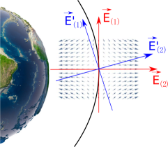
Figure 1: Take the ascending node as the sample point. In the orbital plane, the Newtonian tidal field at this point are plotted. Due to the geodetic effect, the bases $\vec{E}_{(1)}$ and $\vec{E}_{(2)}$ will precess to $\vec{E}^{\prime}_{(1)}$ and $\vec{E}^{\prime}_{(2)}$ after one turn along the orbit. Therefore, the Newtonian tidal forces along the bases will change gradually with time due to the continuous precession of the orientation of the bases relative to the local Newtonian tidal field, which, in the limit $\frac{\tau}{a}\ll\frac{1}{M\omega}$, will result in the geodetic part of the secular tidal forces.

In this paper, we extend the analysis by including the frame-dragging effect. Unlike in Mashhoon1989 which considered the inertial frame defined by remote stars, we now consider the local inertial frame defined by a set of on-board gyros. Due to the precessing rate difference between the local frame and the orbital plane, the relative orientation between the local freely falling frame and the sidereal frame will change gradually with time. Therefore, the Newtonian tidal forces along the bases $E_{(i)}^{\ \ \ \mu}(\tau)$ will be modulated by such an orientation change, which results in the secular parts of the total tidal tensor. Such secular tidal effects can be divided into two different parts according to their origins: the secular tensors $K_{(a)(b)}^{G}$ and $K_{(a)(b)}^{FD}$ generated respectively by the geodetic precession and frame-dragging precession. This is illustrated in Figs. 1 and 2.

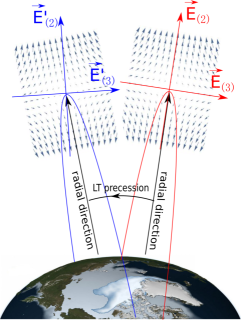
Figure 2: Again, take the ascending nodes as sample points, whose location will precess along the equator due to the LT precession of the orbit. In the equatorial plane, the Newtonian tidal fields at these two ascending nodes are plotted. Due to the frame-dragging effect, the bases will undergo the Schiff precession with an angular rate different from that of the LT precession of the orbit. Therefore, the orientation of the bases relative to the local Newtonian tidal field will be altered gradually, which, in the limit $\frac{\tau}{a}\ll\frac{a^{2}}{J}$, produces secular changes of the Newtonian tidal forces along these bases.

At the 1PN level, and in the limit compared to the periods of the geodetic and frame-dragging precession, that $\frac{\tau}{a}\ll\frac{1}{M\omega}$ and $\frac{\tau}{a}\ll\frac{a^{2}}{J}$, we have

$$K_{(i)(j)}^{G}=\frac{9M^{2}\Psi}{2a^{4}}\left(\begin{array}[]{ccc}\sin 2\Psi&\cos 2\Psi&0\\ \\ \cos 2\Psi&-\sin 2\Psi&0\\ \\ 0&0&0\end{array}\right),$$ (22a)

$$K_{(i)(j)}^{FD}$$

$$=\frac{9JM}{a^{6}\omega}\left(\begin{array}[]{ccc}-\Psi\cos i\sin 2\Psi&-\Psi\cos i\cos 2\Psi&-\frac{1}{4}\sin i(\Psi\sin 2\Psi-\cos 2\Psi+1)\\ \\ -\Psi\cos i\cos 2\Psi&\Psi\cos i\sin 2\Psi&-\frac{1}{4}\sin i[\Psi(\cos 2\Psi+1)+\sin 2\Psi]\\ \\ -\frac{1}{4}\sin i(\Psi\sin 2\Psi-\cos 2\Psi+1)&-\frac{1}{4}\sin i[\Psi(\cos 2\Psi+1)+\sin 2\Psi]&0\end{array}\right).$$ (22g)

(22h)

The above secular tidal tensor $K^{FD}_{(i)(j)}$ from frame-dragging effect does not agree exactly with the results from Mashhoon and Theiss Mashhoon1982 ; Mashhoon1985 ; Theiss1985 that are summarized in Eq. (12) of Paik2008 . To check the validity of these results, one should notice that, when the local, freely falling frame and the sidereal frame coincide at the initial point $\vec{x}=0$ and $\Psi=0$, the secular tensors $K^{G}_{(i)(j)}$ and $K^{FD}_{(i)(j)}$ should vanish. This condition is exactly satisfied by our result when $\Psi=0$ is substituted into Eqs. (22a) and (22h). However, such a self-consistency check is not fully satisfied for the results from Mashhoon and Theiss.

IV Tidal tensor in the Earth-pointing local frame

The Earth-pointing orientation of the S/C (local frame) is another feasible option for satellite gradiometry. Strictly speaking, at the 1PN level, the exact freely falling Earth-pointing frame exists only for polar orbits. Along inclined orbits, there will always be periodic nutations of the local frame (S/C) within the orbital plane due to the frame-dragging effect. Therefore, without attitude control, freely falling Earth-pointing frame is only an approximation at the 1PN level.

Now, we first work out the 1PN tetrad $e_{(a)}^{\ \ \ \mu}$ determining the approximate Earth-pointing frame along the orbit, Eqs .(6). The initial values of the spatial bases $\vec{e}_{(i)}(0)$ are set to be the same as in Eqs. (15). To obtain its Earth-pointing orientation approximately, the local frame (S/C) is set to roll about the transverse axis $\vec{e}_{(3)}$ with an initial angular velocity $w_{0}$ relative to the Fermi normal frame. Considering the uniform geodetic precession of the local frame, we set

$$w_{0}=\omega(1-\frac{3M}{2a}).$$ (23)

Then, following the same method used in the last section, the matrix $e_{(a)}^{\ \ \ \mu}$ and its inverse $e_{\ \ \ \mu}^{(a)}$ can be derived to the required order, the result is given in Eqs. (50) and (65) in Appendix. A

From Eq. (10), $T_{(0)(a)}=0$, and the Newtonian, 1PN GE and GM parts of the total tidal tensor $T_{(i)(j)}$ are found to be

$$T^{N}{}_{(i)(j)}=\left(\begin{array}[]{ccc}\frac{M}{a^{3}}-\omega^{2}&0&0\\ \\ 0&-\omega^{2}-\frac{2M}{a^{3}}&0\\ \\ 0&0&\frac{M}{a^{3}}\end{array}\right),$$ (24a)

$$T^{GE}{}_{(i)(j)}=$$

$$\left(\begin{array}[]{ccc}-\frac{\omega^{4}a^{6}-4M\omega^{2}a^{3}+3M^{2}}{a^{4}}&0&0\\ \\ 0&\frac{7M^{2}-M\omega^{2}a^{3}}{a^{4}}&0\\ \\ 0&0&\frac{3M\omega^{2}a^{3}-3M^{2}}{a^{4}}\end{array}\right),$$ (24g)

(24h)

$$T^{GM}{}_{(i)(j)}=$$

$$\frac{3J\omega}{a^{3}}\left(\begin{array}[]{ccc}0&0&\sin i\cos\Psi\\ \\ 0&2\cos i&-3\sin i\sin\Psi\\ \\ \sin i\cos\Psi&-3\sin i\sin\Psi&-2\cos i\end{array}\right).$$ (24n)

(24o)

Again, these results agree to the 1PN level with the tidal tensors obtained by Mashhoon, Paik and Will Mashhoon1989 for the Earth-pointing frame. As the geodetic precession of the bases is absorbed into their rotations about the axis $e_{(3)}^{\ \ \ \mu}$, there is no secular part in $T_{(i)(j)}$ produced by the geodetic precession as for the inertially guided case. However, an error $\delta\omega_{0}$ in the initial rolling velocity of the S/C will produce a secular tidal field of order $\mathcal{O}(\frac{M}{a^{3}}\tau\delta\omega_{0})$ in the $e_{(1)}^{\ \ \ \mu}-e_{(2)}^{\ \ \ \mu}$ plane (orbital plane), which could be used to adjust the attitude of the S/C in that plane. The effects and errors produced by the uncertainties in the angular velocity of the S/C relative to its mass center will be left to future studies.

If the S/C is forced to strictly follow the Earth-pointing frame by attitude control, there will be no secular terms. However, if the attitude is controlled by on-board gyros, there will be frame-dragging terms due to the Schiff precession of the gyro axes. In the limit $\frac{\tau}{a}\ll\frac{a^{2}}{J}$, the frame-dragging part of the secular tidal tensor can be shown to be

$$T^{FD}{}_{(i)(j)}=\frac{9JM}{a^{6}\omega}\left(\begin{array}[]{ccc}0&-\Psi\cos i&0\\ \\ -\Psi\cos i&0&-\frac{1}{2}\sin i(\Psi\cos\Psi+\sin\Psi)\\ \\ 0&-\frac{1}{2}\sin i(\Psi\cos\Psi+\sin\Psi)&0\end{array}\right).$$ (30)

V Concluding remarks

In this paper, we have derived the complete 1PN tidal tensor, including secular tensors, along 1PN nearly circular orbits under both inertially guided and Earth-pointing frames. At the 1PN level, these secular tidal forces are not new (resonance) effects produced by a rotating source. From our analysis, we find a simple physical picture: the Newtonian tidal forces along certain bases are modulated due to the relativistic precession of the local frame relative to the sidereal frame, which results in different secular terms in the tidal tensor. Nevertheless, the existence of the secular tidal terms does provide the possibility of measuring the GM effect with a great accuracy in satellite gradiometry missions Theiss1985 , although such an experiment would require rather precise gyros Mashhoon1982 .

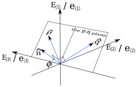
Figure 3: The two perpendicular axes $\hat{\mathbf{p}}$ and $\hat{\mathbf{q}}$ are symmetric with respect to the $E_{(1)}^{\ \ \ \mu}-E_{(2)}^{\ \ \ \mu}$ or $e_{(1)}^{\ \ \ \mu}-e_{(2)}^{\ \ \ \mu}$ plane, and $\hat{\mathbf{n}}$ is orthogonal to the $\hat{\mathbf{p}}-\hat{\mathbf{q}}$ plane. The angle between $\hat{\mathbf{n}}$ and $-\hat{\mathbf{r}}$ is denoted by $\phi$.

In conclusion, we summarize here the gradiometer readout of the frame-dragging part of the secular tidal tensor by a 3-axis gradiometer. Following Mashhoon1989 , we orient two of the three gradiometer axes 45 degrees above and below the orbital plane and difference their outputs to reject the Newtonian and GE terms and measure only the GM and frame-dragging terms, as shown in Fig. 3. In the local frame $E_{(i)}^{\ \ \ \mu}$ or $e_{(i)}^{\ \ \ \mu}$, the three axes of the gradiometer, $\hat{\mathbf{n}},$ $\hat{\mathbf{p}}$ and $\hat{\mathbf{q}}$, are oriented as

$$\hat{\mathbf{n}} = \left(\begin{array}[]{c}\sin\phi\\ -\cos\phi\\ 0\end{array}\right),$$ (31d)

$$\hat{\mathbf{p}} = \frac{1}{\sqrt{2}}\left(\begin{array}[]{c}\cos\phi\\ \sin\phi\\ -1\end{array}\right),$$ (31h)

$$\hat{\mathbf{q}} = \frac{1}{\sqrt{2}}\left(\begin{array}[]{c}\cos\phi\\ \sin\phi\\ 1\end{array}\right).$$ (31l)

In the inertially guided and Earth-pointing frames, the frame-dragging secular terms can be obtained in the difference between the readouts in the $\hat{\mathbf{p}}$ and $\hat{\mathbf{q}}$ axes. For the inertially guided case, the gradiometer measures

$$\frac{1}{2}(K_{\hat{\mathbf{p}}\hat{\mathbf{p}}}-K_{\hat{\mathbf{q}}\hat{\mathbf{q}}})$$ (32)

$$= \boxed{\frac{9JM\Psi\sin i\cos\Psi\sin(\Psi+\phi)}{2a^{6}\omega}}$$

$$-\frac{9JM\sin i\cos(2\Psi+\phi)}{4a^{6}\omega}-\frac{6J\omega\sin i\cos(2\Psi+\phi)}{a^{3}}$$

$$+\frac{9JM\sin i\cos\phi}{4a^{6}\omega}+\frac{3J\omega\sin i\cos(\phi)}{a^{3}}.$$

For the Earth-pointing case, the gradiometer measures

$$\frac{1}{2}(T_{\hat{\mathbf{p}}\hat{\mathbf{p}}}-T_{\hat{\mathbf{q}}\hat{\mathbf{q}}})$$ (33)

$$= \boxed{\frac{9JM\Psi\sin i\sin\phi\cos\Psi}{2a^{6}\omega}}+\frac{9JM\sin i\sin\phi\sin\Psi}{2a^{6}\omega}$$

$$+\frac{9J\omega\sin i\sin\phi\sin\Psi}{a^{3}}-\frac{3J\omega\sin i\cos\phi\cos\Psi}{a^{3}}.$$

The boxed terms are the expected signals from secular terms. A detailed analysis of the errors arising from misalignment and mispointing of the gradiometer axes can be found in Paik2008 .

Appendix A Christoffel symbols and tetrad matrices

As a reference, under the PN coordinate system defined in Sec. II, we give the expressions of the components of the Christoffel symbols $\Gamma_{\>\>\nu\mu}^{\lambda}$:

$$\Gamma_{\ \ \ 0\mu}^{0}=\frac{M}{r^{3}}\left(\begin{array}[]{c}0\\ x^{1}\\ x^{2}\\ x^{3}\end{array}\right),$$ (34a)

$$\Gamma_{\ \ \ 0j}^{i}=$$

$$\left(\begin{array}[]{ccc}0&-\frac{J\left((x^{1})^{2}+(x^{2})^{2}-2(x^{3})^{2}\right)}{r^{5}}&-\frac{3Jx^{2}x^{3}}{r^{5}}\\ \\ \frac{J\left((x^{1})^{2}+(x^{2})^{2}-2(x^{3})^{2}\right)}{r^{5}}&0&\frac{3Jx^{1}x^{3}}{r^{5}}\\ \\ \frac{3Jx^{2}x^{3}}{r^{5}}&-\frac{3Jx^{1}x^{3}}{r^{5}}&0\end{array}\right),$$ (34g)

(34h)

$$\Gamma_{\ \ \ ij}^{1}=-\frac{M}{r^{3}}\left(\begin{array}[]{ccc}x^{1}&x^{2}&x^{3}\\ x^{2}&-x^{1}&0\\ x^{3}&0&-x^{1}\end{array}\right),$$ (34i)

$$\Gamma_{\ \ \ ij}^{2}=-\frac{M}{r^{3}}\left(\begin{array}[]{ccc}-x^{2}&x^{1}&0\\ x^{1}&x^{2}&x^{3}\\ 0&x^{3}&-x^{2}\end{array}\right),$$ (34j)

$$\Gamma_{\ \ \ ij}^{3}=-\frac{M}{r^{3}}\left(\begin{array}[]{ccc}-x^{3}&0&x^{1}\\ 0&-x^{3}&x^{2}\\ x^{1}&x^{2}&x^{3}\end{array}\right),$$ (34k)

$$\Gamma_{\ \ \ ij}^{0}=$$

$$\left(\begin{array}[]{ccc}\frac{6J\left(x^{2}(x^{1})^{3}+x^{2}\left((x^{2})^{2}+(x^{3})^{2}\right)x^{1}\right)}{r^{7}}&\frac{3J\left(-(x^{3})^{2}(x^{1})^{2}-(x^{1})^{4}+(x^{2})^{2}\left((x^{2})^{2}+(x^{3})^{2}\right)\right)}{r^{7}}&\frac{3J\left(x^{2}x^{3}(x^{1})^{2}+x^{2}x^{3}\left((x^{2})^{2}+(x^{3})^{2}\right)\right)}{r^{7}}\\ \\ \\ \frac{3J\left(-(x^{3})^{2}(x^{1})^{2}-(x^{1})^{4}+(x^{2})^{2}\left((x^{2})^{2}+(x^{3})^{2}\right)\right)}{r^{7}}&-\frac{6J\left(x^{2}(x^{1})^{3}+x^{2}\left((x^{2})^{2}+(x^{3})^{2}\right)x^{1}\right)}{r^{7}}&-\frac{3J\left(x^{3}(x^{1})^{3}+x^{3}\left((x^{2})^{2}+(x^{3})^{2}\right)x^{1}\right)}{r^{7}}\\ \\ \\ \frac{3J\left(x^{2}x^{3}(x^{1})^{2}+x^{2}x^{3}\left((x^{2})^{2}+(x^{3})^{2}\right)\right)}{r^{7}}&-\frac{3J\left(x^{3}(x^{1})^{3}+x^{3}\left((x^{2})^{2}+(x^{3})^{2}\right)x^{1}\right)}{r^{7}}&0\end{array}\right).$$ (34s)

(34t)

To the required order, the transformation matrices between the local Earth-pointing frame and the Earth-centered PN coordinate system $e_{(a)}^{\ \ \ \mu}$ and $e_{\ \ \ \mu}^{(a)}$ can be shown to be

$$e_{(a)}^{\ \ \ \mu}=$$

$$\left(\begin{array}[]{cccc}1+\frac{a^{2}\omega^{2}}{2}+\frac{M}{a}&-a\omega\sin\Psi&a\omega\cos i\cos\Psi&a\omega\sin i\cos\Psi\\ &-\frac{2J\cos i(\Psi\cos\Psi+\sin\Psi)}{a^{2}}&+\frac{2J(\cos\Psi-\Psi\sin\Psi)}{a^{2}}\\ \\ \\ (a+2M)\omega&-(1+\frac{a^{2}\omega^{2}}{2}-\frac{M}{a})\sin\Psi&(1+\frac{a^{2}\omega^{2}}{2}-\frac{M}{a})\cos i\cos\Psi&(1+\frac{a^{2}\omega^{2}}{2}-\frac{M}{a})\sin i\cos\Psi\\ &+\frac{J\Psi\cos i\cos\Psi}{a^{3}\omega}&+\frac{J\Psi\left(1+3\cos i\right)\sin\Psi}{4a^{3}\omega}&+\frac{3J\Psi\sin i\sin\Psi}{4a^{3}\omega}\\ \\ \\ -\frac{3J\Psi\cos i}{a^{2}}&(1-\frac{M}{a})\cos\Psi&(1-\frac{M}{a})\cos i\sin\Psi&(1-\frac{M}{a})\sin i\sin\Psi\\ &+\frac{J\Psi\cos i\sin\Psi}{a^{3}\omega}&-\frac{\left(1+3\cos 2i\right)J\Psi\cos\Psi}{4a^{3}\omega}-\frac{3J\sin^{2}i\sin\Psi}{2a^{3}\omega}&-\frac{3J\sin 2i\left(\Psi\cos\Psi-\sin\Psi\right)}{4a^{3}\omega}\\ \\ \\ -\frac{3J\Psi\sin i\sin\Psi}{2a^{2}}&\frac{J\sin i\left(3\sin 2\Psi-2\Psi\right)}{4a^{3}\omega}&(1-\frac{M}{a})\sin i&-(1-\frac{M}{a})\cos i\\ &&+\frac{3J\sin i\cos i\sin^{2}\Psi}{2a^{3}\omega}&+\frac{3J\sin^{2}i\sin^{2}\Psi}{2a^{3}\omega}\end{array}\right),$$ (49)

(50)

$$e_{\ \ \ \mu}^{(a)}=$$

$$\left(\begin{array}[]{cccc}1+\frac{a^{2}\omega^{2}}{2}-\frac{M}{a}+\frac{2J\omega\cos i}{a}&-a\omega+\frac{M^{2}\omega}{a}-\frac{2J\cos i}{a^{2}}&\frac{3J\Psi\cos i}{a^{2}}&\frac{J\sin i(3\Psi\sin\Psi-4\cos\Psi)}{2a^{2}}\\ \\ \\ (a+2M)\omega\sin\Psi&-(1+\frac{a^{2}\omega^{2}}{2}+\frac{M}{a})\sin\Psi&(1+\frac{M}{a})\cos\Psi&\frac{3J\sin i\sin\Psi}{4a^{3}\omega}-\frac{J\Psi\sin i}{2a^{3}\omega}\\ +\frac{2J\Psi\cos i\cos\Psi}{a^{2}}&+\frac{J\Psi\cos i\cos\Psi}{a^{3}\omega}&+\frac{J\Psi\cos i\sin\Psi}{a^{3}\omega}\\ \\ \\ -(a+2M)\omega\cos i\cos\Psi&(1+\frac{a^{2}\omega^{2}}{2}+\frac{M}{a})\cos i\cos\Psi&(1+\frac{M}{a})\cos i\sin\Psi&(1+\frac{M}{a})\sin i\\ +\frac{2J\Psi\sin\Psi}{a^{2}}&+\frac{3J\Psi\cos 2i\sin\Psi}{4a^{3}\omega}+\frac{J\Psi\sin\Psi}{4a^{3}\omega}&-\frac{3J\sin^{2}i\sin\Psi}{2a^{3}\omega}-\frac{J\Psi(3\cos 2i+1)\cos\Psi}{4a^{3}\omega}&+\frac{3J\sin i\cos i\sin^{2}\Psi}{2a^{3}\omega}\\ \\ \\ -(a+2M)\omega\sin i\cos\Psi&(1+\frac{a^{2}\omega^{2}}{2}+\frac{M}{a})\sin i\cos\Psi&(1+\frac{M}{a})\sin i\sin\Psi&-(1+\frac{M}{a})\cos i\\ &+\frac{3J\Psi\sin i\cos i\sin\Psi}{2a^{3}\omega}&-\frac{3J\sin i\cos i(3\Psi\cos\Psi-\sin\Psi)}{2a^{3}\omega}&+\frac{3J\sin^{2}i\sin^{2}\Psi}{2a^{3}\omega}\end{array}\right).$$ (64)

(65)

References

• (1) R. Rummel, W. Yi, and C. Stummer, J. Geodesy 85, 777 (2011).
• (2) C. E. Griggs, H. J. Paik, M. V. Moody, S.-C. Han, D. D. Rowlands, F. G. Lemoine, P. J. Shirron, and X. Li, in Proceedings of the 46th Lunar and Planetary Conference (Houston, 2015), p.1735.
• (3) G. M. Tino, F. Sorrentino, D. Aguilera, B. Battelier, A. Bertoldi, Q. Bodart, K. Bongs, P. Bouyer, C. Braxmaier, L. Cacciapuoti, N. Gaaloul, N. Gürlebeck, M. Hauth, S. Herrmann, M. Krutzik, A. Kubelka, A. Landragin, A. Milke, A. Peters, E. M. Rasel, E. Rocco, C. Schubert, T. Schuldt, K. Sengstock, and A. Wicht, Nucl. Phys. B Proc. Suppl. 243, 203 (2013).
• (4) O. Carraz, C. Siemes, L. Massotti, R. Haagmans, and P. Silvestrin, Sci. Tech. 26, 139 (2014).
• (5) H. J. Paik, B. Mashhoon, and C. M. Will, in Experimental Gravitational Physics, edited by P. F. Michelson, H. En-Ke, and G. Pizzella (1988), pp. 229-244.
• (6) B. Mashhoon, H. J. Paik, and C. M. Will, Phys. Rev. D 39, 2825 (1989).
• (7) K. S. Thorne, in Near Zero: New Frontiers of Physics, edited by J. D. Fairbank, B. S. Deaver, Jr., C. W. F. Everitt, and P. F. Michelson (1988), pp. 573-586.
• (8) R. Maartens and B. A. Bassett, Class. Quant. Grav. 15, 705 (1998).
• (9) B. Mashhoon, ArXiv General Relativity and Quantum Cosmology e-prints (2003), arXiv:gr-qc/0311030.
• (10) R. H. Dicke, Relativity, Groups and Topology (Gordon and Breach, 1964), pp. 165-313.
• (11) C. M. Will, Living Rev. Relativity 17, (2014), 10.12942/lrr-2014-4.
• (12) D. W. Sciama, Mon. Not. Roy. Astron. Soc. 113, 34 (1953).
• (13) I. Ciufolini and J. A. Wheeler, Gravitation and Inertia (Princeton University Press, 1995).
• (14) C. W. F. Everitt, D. B. Debra, B. W. Parkinson, J. P. Turneaure, J. W. Conklin, M. I. Heifetz, G. M. Keiser, A. S. Silbergleit, T. Holmes, J. Kolodziejczak, M. Al-Meshari, J. C. Mester, B. Muhlfelder, V. G. Solomonik, K. Stahl, P. W. Worden, Jr., W. Bencze, S. Buchman, B. Clarke, A. Al-Jadaan, H. Al-Jibreen, J. Li, J. A. Lipa, J. M. Lockhart, B. Al-Suwaidan, M. Taber, and S.Wang, Phys. Rev. Lett. 106, 221101 (2011).
• (15) L. I. Schiff, Proc. Nat. Acad. Sci. 46, 871 (1960).
• (16) J. Lense and H. Thirring, Z. Phys. 19, 156 (1918).
• (17) I. Ciufolini, Phys. Rev. Lett. 56, 278 (1986).
• (18) http://science.nasa.gov/missions/champ/
• (19) http://op.gfz-potsdam.de/grace/results/grav/g002_eigen-grace02s.html
• (20) I. Ciufolini and E. Pavlis, Nature 431, 958 (2004).
• (21) I. Ciufolini, Nature 449, 41 (2007).
• (22) V. B. Braginskii and A. G. Polnarev, Pis’ma Zh. Eksp. Teor. Fiz. 31, 444 (1980).
• (23) B. Mashhoon and D. S. Theiss, Phys. Rev. Lett. 49, 1542 (1982).
• (24) H. J. Paik, Adv. Space Res. 9, 41 (1989).
• (25) http://sci.esa.int/lisa-pathfinder/
• (26) P. Xu, L.-E. Qiang, P. Dong, X.-F. Gong, G. Heinzel, Z.-R. Luo, H. J. Paik, W.-L. Tang, W. J. Weber, and Y.-K. Lau, Precision measurement of planetary gravitomagnetic field in general relativity with laser interferometry in space — Theoretical foundation (To be published).
• (27) B. Mashhoon, Gen. Rel. Grav. 16, 311 (1984).
• (28) B. Mashhoon, Found. Phys. 15, 497 (1985).
• (29) B. Mashhoon and D. S. Theiss, Phys. Lett. A 115, 333 (1986).
• (30) D. S. Theiss, Phys. Lett. A 109, 19 (1985).
• (31) E. Gill, J. Schastok, M. H. Soffel, and H. Ruder, Phys. Rev. D 39, 2441 (1989).
• (32) C. A. Blockley and G. E. Stedman, Phys. Lett. A 147, 161 (1990).
• (33) S. Weinberg, Gravitation and Cosmology: Principles and Applications of the General Theory of Relativity (John Wiley & Sons, Inc., 1972).
• (34) N. Straumann, General Relativity and Relativistic Astrophysics (Springer-Verlag, 1984).
• (35) X.-Q. Li, M.-X. Shao, H. J. Paik, Y.-C. Huang, T.-X. Song, and X. Bian, Gen. Rel. Grav. 46, 1 (2014).
• (36) G. Petit and B. Luzum, IERS Technical Note 36, 1 (2010).
• (37) R. M. Wald, General Relativity (University of Chicago Press, 1984).
• (38) H. J. Paik, Gen. Rel. Grav. 40, 907 (2008).