Admissible colourings of 3-manifold triangulations for Turaev-Viro type invariants

Abstract

Turaev Viro invariants are amongst the most powerful tools to distinguish $3$-manifolds: They are implemented in mathematical software, and allow practical computations. The invariants can be computed purely combinatorially by enumerating colourings on the edges of a triangulation $\mathfrak{T}$.

These edge colourings can be interpreted as embeddings of surfaces in $\mathfrak{T}$. We give a characterisation of how these embedded surfaces intersect with the tetrahedra of $\mathfrak{T}$. This is done by characterising isotopy classes of simple closed loops in the $3$-punctured disk. As a direct result we obtain a new system of coordinates for edge colourings which allows for simpler definitions of the tetrahedron weights incorporated in the Turaev-Viro invariants.

Moreover, building on a detailed analysis of the colourings, as well as classical work due to Kirby and Melvin, Matveev, and others, we show that considering a much smaller set of colourings suffices to compute Turaev-Viro invariants in certain significant cases. This results in a substantial improvement of running times to compute the invariants, reducing the number of colourings to consider by a factor of $2^{n}$. In addition, we present an algorithm to compute Turaev-Viro invariants of degree four – a problem known to be $\#P$-hard – which capitalises on the combinatorial structure of the input.

The improved algorithms are shown to be optimal in the following sense: There exist triangulations admitting all colourings the algorithms consider. Furthermore, we demonstrate that our new algorithms to compute Turaev-Viro invariants are able to distinguish the majority of $\mathbb{Z}$-homology spheres with complexity up to $11$ in $O(2^{n})$ operations in $\mathbb{Q}$.

Keywords: geometric topology, triangulations of $3$-manifolds, Turaev-Viro invariants, combinatorial algorithms

1 Introduction

In geometric topology, recognising the topological type of a given manifold, i.e., testing if two manifolds are equivalent, is one of the most fundamental algorithmic problems. In fact, the task of comparing the topology of two given manifolds often stands at the very beginning of a question, and solving it is essential for conducting research in the field.

Depending on the dimension of the manifolds, this task is remarkably difficult to solve in general. There exists an algorithmic solution in dimension three due to Perelman’s proof of the geometrisation conjecture [14], but it is highly theoretical in nature and has never been implemented. Moreover, in dimensions $\geq 5$ the problem becomes undecidable [20].

As a result, comparing the topology of two manifolds in dimension $\geq 3$ often requires human-machine interactions, combining various strategies. In practice, these are largely of two distinct types: (i) computing invariants in order to prove that two given manifolds are distinct; and (ii) trying to establish a certificate that two given manifolds are homeomorphic.

Here we focus on the former type of methods, more precisely, on a particularly powerful family of invariants for $3$-manifolds, called the Turaev-Viro invariants [22]. These are parameterised by two integers $r$ and $q$, with $r\geq 3$, $0<q<2r$, and denoted by $\mathrm{TV}_{r,q}$. They derive from quantum field theory but can be computed by purely combinatorial means—much like the famous Jones polynomial for knots. Implementations exists for $3$-manifolds represented by (i) spines ($2$-dimensional skeletons of $3$-manifolds) in Matveev’s Manifold Recogniser [15, 16]; and (ii) triangulations (a list of tetrahedra with their triangular faces glued together in pairs) in Burton’s software Regina [5, 6].

We work within the latter setting, namely triangulations of $3$-manifolds $\mathfrak{T}$, where the definition of the Turaev-Viro invariant $\mathrm{TV}_{r,q}$ is based on admissible colourings of the edges of $\mathfrak{T}$ with $r-1$ distinct colours. Each admissible colouring defines a weight, and $\mathrm{TV}_{r,q}(\mathfrak{T})$ equals the sum of these weights. The naive implementation of this procedure is simple, efficient in memory, but has worst case running time $(r-1)^{n+v}$, where $n$ is the number of tetrahedra and $v$ the number of vertices of $\mathfrak{T}$. More recently, Burton and the authors introduced a fixed parameter tractable (FPT) algorithm which is linear in $n$, and only singly exponential in the treewidth of the dual graph of $\mathfrak{T}$ [6].

In this article, we study admissible colourings of $3$-manifold triangulations with the aim of a better understanding of Turaev-Viro invariants and significant algorithmic improvements.

Admissible colourings can be interpreted as surfaces embedded in a triangulated $3$-manifold, where the colour of an edge corresponds to (half) its number of intersections with the surface, and the surface intersects the triangles of the triangulation in straight arcs. Embedded surfaces play a vital role in $3$-manifold topology, most notably due to Haken’s theory of normal surfaces, i.e. embedded surfaces intersecting the tetrahedra of a triangulation in a collection of triangles and quadrilaterals [8]. Surfaces of critical importance to the topology of a manifold, such as a disk bounding an unknot in a triangulation of a knot-complement, can be proven to occur as a normal surface. For other problems, such as recognising the $3$-sphere, surfaces of slightly more general types have to be considered [18]. Surfaces coming from admissible colourings contain all these surface types and many more (depending on the value of $r$). See recent work by Bachman [1] for a study of such surfaces of arbitrary index from a topological point of view. This illustrates the potential power of the Turaev-Viro invariants in distinguishing between non-homeomorphic $3$-manifolds, based on purely combinatorial objects.

We present a classification of surface types defined by admissible colourings in form of isotopy classes of simple closed loops in the $3$-punctured disk (as a model of the tetrahedron). We give a combinatorial characterisation of this bijection using intersection numbers of the surface with the six edges of a tetrahedron. As an application of this characterisation we transform and simplify the formulae for the tetrahedra weights for $\mathrm{TV}_{r,q}$, in terms of the surface pieces intersecting a tetrahedron.

Moreover, we build on work by Kirby and Melvin [12] and Matveev [15] to bound the number of admissible colourings relative to the size, the number of vertices, and the first Betti number of a triangulation. In particular, we prove sharp upper bounds on the number of admissible colourings which are much smaller than the trivial upper bound, and which are strongest for triangulations of homology spheres with only one vertex. In addition, we obtain a new upper bound for the size of $\mathrm{Adm}(\mathfrak{T},4)$ depending on the specific structure of the input triangulation, which is sharp in many cases. Note that this is particularly interesting since computing $\mathrm{TV}_{4,1}$ is a $\#P$-hard problem [6, 13].

We use these bounds together with classical results from $3$-manifold topology to obtain a significant exponential speed-up of the computation of some Turaev-Viro invariants. In particular, we reduce running times of the naive enumeration procedure from $(r-1)^{n+v}$ to $O(\lceil(r-1)/2\rceil^{n+1})$ for $r$ odd and $q=1$; and describe an enumeration procedure to compute $\mathrm{TV}_{4,1}$ which is shown to be near-optimal in most cases of small $3$-manifold triangulations.

Note that the improved algorithms still have exponential running times. However, we give experimental evidence that the reduction in the base of the exponent is of practical significance for triangulations of intermediate size, and $4\leq r\leq 9$. This range of values is highly relevant for major applications such as building censuses of minimal triangulations.

2 Background

2.1 Manifolds, triangulations, and (co-)homology groups

Let $M$ be a closed $3$-manifold. A generalised triangulation $\mathfrak{T}$ of $M$ is a collection of $n$ abstract tetrahedra $\Delta_{1},\ldots,\Delta_{n}$ together with $2n$ gluing maps identifying their $4n$ triangular faces in pairs, such that the underlying topological space is homeomorphic to $M$.

As a consequence of the gluings, vertices, edges or triangles of the same tetrahedron may be identified. Indeed, it is common in practical applications to have a one-vertex triangulation, in which all vertices of all tetrahedra are identified to a single point. We refer to an equivalence class defined by the gluing maps as a single face of the triangulation.

Generalised triangulations are widely used in $3$-manifold topology. They are closely related, but more general, than simplicial complexes: every simplicial complex triangulating a manifold is a generalised triangulation, and some subdivision of a generalised triangulation is always a simplicial complex.

Let $\mathfrak{T}$ be a generalised $3$-manifold triangulation. For the field of coefficients $\mathbb{Z}_{2}:=\mathbb{Z}/2\mathbb{Z}$, the group of $p$-chains, $0\leq p\leq 3$, denoted $\mathbf{C}_{p}(\mathfrak{T},\mathbb{Z}_{2})$, of $\mathfrak{T}$ is the group of formal sums of $p$-faces with $\mathbb{Z}_{2}$ coefficients. The boundary operator is a linear operator $\partial_{p}:\mathbf{C}_{p}(\mathfrak{T},\mathbb{Z}_{2})\rightarrow\mathbf{C}_{p-1}(\mathfrak{T},\mathbb{Z}_{2})$ such that $\partial_{p}\sigma=\partial_{p}\{v_{0},\cdots,v_{p}\}=\sum_{j=0}^{p}\{v_{0},\cdots,\widehat{v_{j}},\cdots,v_{p}\}$, where $\sigma$ is a face of $\mathfrak{T}$, $\{v_{0},\ldots,v_{p}\}$ represents $\sigma$ as a face of a tetrahedron of $\mathfrak{T}$ in local vertices $v_{0},\ldots,v_{p}$, and $\widehat{v_{j}}$ means $v_{j}$ is deleted from the list. Denote by $\mathbf{Z}_{p}(\mathfrak{T},\mathbb{Z}_{2})$ and $\mathbf{B}_{p-1}(\mathfrak{T},\mathbb{Z}_{2})$ the kernel and the image of $\partial_{p}$ respectively. Observing $\partial_{p}\circ\partial_{p+1}=0$, we define the $p$-th homology group $\mathbf{H}_{p}(\mathfrak{T},\mathbb{Z}_{2})$ of $\mathfrak{T}$ by the quotient $\mathbf{H}_{p}(\mathfrak{T},\mathbb{Z}_{2})=\mathbf{Z}_{p}(\mathfrak{T},\mathbb{Z}_{2})/\mathbf{B}_{p}(\mathfrak{T},\mathbb{Z}_{2})$. These structures are vector spaces. Informally, the $p$-th homology group, $0\leq p\leq 3$, of a generalised triangulation $\mathfrak{T}$ counts the number of “$p$-dimensional holes” in $\mathfrak{T}$.

The concept of cohomology is in many ways dual to homology, but more abstract and endowed with more algebraic structure. It is defined in the following way: The group of $p$-cochains $\mathbf{C}^{p}(\mathfrak{T},\mathbb{Z}_{2})$ is the formal sum of linear maps of $p$-faces of $\mathfrak{T}$ into $\mathbb{Z}_{2}$. The coboundary operator is a linear operator $\delta^{p}:\mathbf{C}^{p-1}(\mathfrak{T},\mathbb{Z}_{2})\rightarrow\mathbf{C}^{p}(\mathfrak{T},\mathbb{Z}_{2})$ such that for all $\phi\in\mathbf{C}^{p-1}(\mathfrak{T},\mathbb{Z}_{2})$ we have $\delta^{p}(\phi)=\phi\circ\partial_{p}$. As above, $p$-cocycles are the elements in the kernel of $\delta^{p+1}$, $p$-coboundaries are elements in the image of $\delta^{p}$, and the $p$-th cohomology group $\mathbf{H}^{p}(\mathfrak{T},\mathbb{Z}_{2})$ is defined as the $p$-cocycles factored by the $d$-coboundaries.

The exact correspondence between elements of homology and cohomology is best illustrated by Poincaré duality stating that for closed $d$-manifold triangulations $\mathfrak{T}$, $\mathbf{H}^{p}(\mathfrak{T},\mathbb{Z}_{2})$ and $\mathbf{H}_{d-p}(\mathfrak{T},\mathbb{Z}_{2})$ are dual as vector spaces. More precisely, let $S$ be a $2$-cycle in $\mathfrak{T}$ representing a class in $\mathbf{H}_{2}(\mathfrak{T},\mathbb{Z}_{2})$. We can perturb $S$ such that it contains no vertex of $\mathfrak{T}$ and intersects every tetrahedron of $\mathfrak{T}$ in a single triangle (separating one vertex from the other three) or a single quadrilateral (separating pairs of vertices). It follows that every edge of $\mathfrak{T}$ intersects $S$ in $0$ or $1$ points. Then the $1$-cochain defined by mapping every edge intersecting $S$ to $1$ and mapping all other edges to $0$ represents the Poincaré dual of $S$ in $\mathbf{H}^{1}(\mathfrak{T},\mathbb{Z}_{2})$.

In this article we will mostly consider the first cohomology group $\mathbf{H}^{1}(\mathfrak{T},\mathbb{Z}_{2})$ —a $\mathbb{Z}_{2}$-vector space of dimension called the first Betti number $\beta_{1}(\mathfrak{T},\mathbb{Z}_{2})$ of $\mathfrak{T}$. (Co)homology groups can be computed on a triangulation in polynomial time. For a more detailed introduction into (co)homology theory see [10].

2.2 Turaev-Viro type invariants

Let $\mathfrak{T}$ be a generalised triangulation of a closed $3$-manifold $M$, and let $r\geq 3$, be an integer. Let $V$, $E$, $F$ and $T$ denote the set of vertices, edges, triangles and tetrahedra of the triangulation $\mathfrak{T}$ respectively. Let $I=\{0,1/2,1,3/2,\ldots,(r-2)/2\}$ be the set of the first $r-1$ non-negative half-integers. A colouring of $\mathfrak{T}$ is defined to be a map $\theta\colon\thinspace E\to I$; that is, $\theta$ “colours” each edge of $\mathfrak{T}$ with an element of $I$. A colouring $\theta$ is admissible if, for each triangle of $\mathfrak{T}$, the three edges $e_{1}$, $e_{2}$, and $e_{3}$ bounding the triangle satisfy the

• parity condition $\theta(e_{1})+\theta(e_{2})+\theta(e_{3})\in\mathbb{Z}$;

• triangle inequalities $\theta(e_{i})\leq\theta(e_{j})+\theta(e_{k})$, $\{i,j,k\}=\{1,2,3\}$; and

• upper bound constraint $\theta(e_{1})+\theta(e_{2})+\theta(e_{3})\leq r-2$.

For a triangulation $\mathfrak{T}$ and a value $r\geq 3$, its set of admissible colourings is denoted by $\mathrm{Adm}(\mathfrak{T},r)$.

For each admissible colouring $\theta$ and for each vertex $u\in V$, edge $e\in E$, triangle $f\in F$ or tetrahedron $t\in T$ we define weights $|u|_{\theta},|e|_{\theta},|f|_{\theta},|t|_{\theta}\in\mathbb{C}$. The weights of vertices are constant, and the weights of edges, triangles and tetrahedra only depend on the colours of edges they are incident to. Using these weights, we define the weight of the colouring to be

$$|\mathfrak{T}|_{\theta}=\prod_{v\in V}|u|_{\theta}\times\prod_{e\in E}|e|_{\theta}\times\prod_{f\in F}|f|_{\theta}\times\prod_{t\in T}|t|_{\theta},$$ (1)

Invariants of Turaev-Viro types of $\mathfrak{T}$ are defined as sums of the weights of all admissible colourings of $\mathfrak{T}$, that is $\mathrm{TV}_{r}(\mathfrak{T})=\sum_{\theta\in\mathrm{Adm}(\mathfrak{T},r)}|\mathfrak{T}|_{\theta}$.

In [22], Turaev and Viro show that, when the weighting system satisfies some identities, $\mathrm{TV}_{r}(\mathfrak{T})$ is indeed an invariant of the manifold; that is, if $\mathfrak{T}$ and $\mathfrak{T}^{\prime}$ are generalised triangulations of the same closed 3-manifold $M$, then $\mathrm{TV}_{r}(\mathfrak{T})=\mathrm{TV}_{r}(\mathfrak{T}^{\prime})$ for all $r$. We will thus sometimes abuse notation and write $\mathrm{TV}_{r}(M)$, meaning the Turaev-Viro invariant computed for a triangulation of $M$. In Section 2.4 we give the precise definition of the weights of the original Turaev-Viro invariant at $sl_{2}(\mathbb{C})$, which not only depend on $r$ but also on a second integer $0<q<2r$. The definition of these weights is rather involved, and the study of admissible colourings in Section 3 allows us to give more comprehensible formulae.

For an $n$-tetrahedra triangulation $\mathfrak{T}$ with $v$ vertices (and thus, necessarily $n+v$ edges), there is a simple backtracking algorithm to compute $\mathrm{TV}_{r}(\mathfrak{T})$ by testing the $(r-1)^{v+n}$ possible colourings for admissibility and computing their weights. The case $r=3$ can however be computed in polynomial time, due to a connection between $\mathrm{TV}_{3}$ and homology [6, 15].

2.3 Turaev-Viro invariants at a cohomology class

Let $\mathbf{H}^{1}(\mathfrak{T},\mathbb{Z}_{2})=(\mathbb{Z}_{2})^{\beta_{1}(\mathfrak{T},\mathbb{Z}_{2})}$ be the cohomology group of $\mathfrak{T}$ in dimension one with $\mathbb{Z}_{2}$ coefficients, and let $\alpha$ be a $1$-cocycle in $\mathfrak{T}$, that is, a representative of an element in $\mathbf{H}^{1}(\mathfrak{T},\mathbb{Z}_{2})$. Following the definition of $1$-cohomology it can be shown that on each triangle, $\alpha$ evaluates to $1$ on none or two of its edges. Thus, by colouring all the edges contained in $\alpha$ by $1/2$ and the remaining ones by $0$, $\alpha$ defines an element in $\mathrm{Adm}(\mathfrak{T},3)$.

Proposition 1

Let $\mathfrak{T}$ be a $3$-manifold triangulation with edge set $E$, $r\geq 3$, and $\theta\in\mathrm{Adm}(\mathfrak{T},r)$. Then the reduction of $\theta$, defined by $\theta^{\prime}:E\to\{0,1/2\};\,\,e\mapsto\theta(e)-\lfloor\theta(e)\rfloor$, is an admissible colouring in $\mathrm{Adm}(\mathfrak{T},3)$.

Proof

Let $f$ be a triangle of $\mathfrak{T}$ with edges $e_{1}$, $e_{2}$, and $e_{3}$. Since $\theta\in\mathrm{Adm}(\mathfrak{T},r)$ is admissible, we have $\theta(e_{1})+\theta(e_{2})+\theta(e_{3})\in\mathbb{Z}$. Thus, there are either no or two half-integers amongst the colours of the edges of $f$ and $\theta^{\prime}\in\mathrm{Adm}(\mathfrak{T},3)$. ∎

Thus every colouring $\theta\in\mathrm{Adm}(\mathfrak{T},r)$ can be associated to a $1$-cohomology class of $\mathfrak{T}$ via its reduction $\theta^{\prime}$. We know from [15, 22] that this construction can be used to split $\mathrm{TV}_{r,q}(\mathfrak{T})$ into simpler invariants indexed by the elements of $\mathbf{H}^{1}(\mathfrak{T},\mathbb{Z}_{2})$. More precisely, let $[\alpha]\in\mathbf{H}^{1}(\mathfrak{T},\mathbb{Z}_{2})$ be a cohomology class, then $\mathrm{TV}_{r}(\mathfrak{T},[\alpha])=\sum_{\theta\in\mathrm{Adm}(\mathfrak{T},r),\theta^{\prime}\in[\alpha]}|\mathfrak{T}|_{\theta}$, where $\theta^{\prime}$ denotes the reduction of $\theta$, is an invariant of $\mathfrak{T}$. The special case $\mathrm{TV}_{r}(\mathfrak{T},[0])$ is of particular importance for computations as explained in further detail in Section 4.

2.4 Weights of the Turaev-Viro invariant at $sl_{2}(\mathbb{C})$

Let $\mathfrak{T}$ be a generalised triangulation of a closed 3-manifold $M$, let $r$ and $q$ be integers with $r\geq 3$, $0<q<2r$, and let $\gcd(r,q)=1$. We define the Turaev-Viro invariant $\mathrm{TV}_{r,q}(\mathfrak{T})$ at $sl_{2}(\mathbb{C})$ as follows.

Let $V$, $E$, $F$ and $T$ denote the set of vertices, edges, triangles and tetrahedra respectively of the triangulation $\mathfrak{T}$. Let $I=\{0,1/2,1,3/2,\ldots,(r-2)/2\}$. For each admissible colouring $\theta$ and for each vertex $v\in V$, edge $e\in E$, triangle $f\in F$ or tetrahedron $t\in T$, we define weights $|v|_{\theta},|e|_{\theta},|f|_{\theta},|t|_{\theta}\in\mathbb{C}$.

Our notation differs slightly from Turaev and Viro [22]; most notably, Turaev and Viro do not consider triangle weights $|f|_{\theta}$, but instead incorporate an additional factor of $|f|_{\theta}^{1/2}$ into each tetrahedron weight $|t|_{\theta}$ and $|t^{\prime}|_{\theta}$ for the two tetrahedra $t$ and $t^{\prime}$ containing $f$. This choice of notation simplifies the notation and avoids unnecessary (but harmless) ambiguities when taking square roots.

Let $\zeta=e^{i\pi q/r}\in\mathbb{C}$. Note that our conditions imply that $\zeta$ is a $(2r)$-th root of unity, and that $\zeta^{2}$ is a primitive $r$-th root of unity; that is, $(\zeta^{2})^{k}\neq 1$ for $k=1,\ldots,r-1$. For each positive integer $i$, we define $[i]=(\zeta^{i}-\zeta^{-i})/(\zeta-\zeta^{-1})$ and, as a special case, $[0]=1$. We next define the “bracket factorial” $[i]!=[i]\,[i-1]\ldots[0]$. Note that $[r]=0$, and thus $[i]!=0$ for all $i\geq r$.

We give each vertex constant weight

$$|v|_{\theta}=\frac{\left|\zeta-\zeta^{-1}\right|^{2}}{2r},$$

and each edge $e$ of colour $i\in I$ (i.e., for which $\theta(e)=i$)

$$|e|_{\theta}=(-1)^{2i}\cdot[2i+1].$$

A triangle $f$ whose three edges have colours $i,j,k\in I$ is assigned the weight

$$|f|_{\theta}=(-1)^{i+j+k}\cdot\frac{[i+j-k]!\cdot[i+k-j]!\cdot[j+k-i]!}{[i+j+k+1]!}.$$

Note that the parity condition and triangle inequalities ensure that the argument inside each bracket factorial is a non-negative integer.

Figure 1: Edge colours of a tetrahedron.

Finally, let $t$ be a tetrahedron with edges colours $i_{0},i_{1},i_{2},i_{3},i_{4},i_{5}$ as indicated in Figure 1. In particular, the four triangles surrounding $t$ have colours $(i_{0},i_{1},i_{3})$, $(i_{0},i_{2},i_{4})$, $(i_{1},i_{2},i_{5})$ and $(i_{3},i_{4},i_{5})$, and the three pairs of opposite edges have colours $(i_{0},i_{5})$, $(i_{1},i_{4})$ and $(i_{2},i_{3})$. We define

$$\tau_{\theta}(t,z) =[z-i_{0}-i_{1}-i_{3}]!\cdot[z-i_{0}-i_{2}-i_{4}]!\cdot[z-i_{1}-i_{2}-i_{5}]!\cdot[z-i_{3}-i_{4}-i_{5}]!\,,$$

$$\kappa_{\theta}(t,z) =[i_{0}+i_{1}+i_{4}+i_{5}-z]!\cdot[i_{0}+i_{2}+i_{3}+i_{5}-z]!\cdot[i_{1}+i_{2}+i_{3}+i_{4}-z]!$$

for all integers $z$ such that the bracket factorials above all have non-negative arguments; equivalently, for all integers $z$ in the range $z^{-}\leq z\leq z^{+}$ with

$$z^{-} =\max\{i_{0}+i_{1}+i_{3},\ i_{0}+i_{2}+i_{4},\ i_{1}+i_{2}+i_{5},\ i_{3}+i_{4}+i_{5}\}\,;$$

$$z^{+} =\min\{i_{0}+i_{1}+i_{4}+i_{5},\ i_{0}+i_{2}+i_{3}+i_{5},\ i_{1}+i_{2}+i_{3}+i_{4}\}.$$

Note that, as before, the parity condition ensures that the argument inside each bracket factorial above is an integer. We then declare the weight of tetrahedron $t$ to be

$$|t|_{\theta}=\sum_{z^{-}\leq z\leq z^{+}}\frac{(-1)^{z}\cdot[z+1]!}{\tau_{\theta}(t,z)\cdot\kappa_{\theta}(t,z)},$$

Note that all weights are polynomials in $\zeta$ with rational coefficients, where $\zeta=e^{i\pi q/r}$. Using these weights, we can define the weight $|\mathfrak{T}|_{\theta}$ of an edge colouring $\theta$ as done in Equation (1), and the Turaev-Viro invariant to be the sum of the weights of all admissible colourings

$$\mathrm{TV}_{r,q}(\mathfrak{T})=\sum_{\theta\ \mathrm{admissible}}|\mathfrak{T}|_{\theta}.$$

3 Admissible colourings of tetrahedra and embedded surfaces

In the definition of Turaev-Viro type invariants, colours are assigned to edges and the admissibility conditions only depend on the triangles. In this section, we translate these conditions into a characterisation of the “admissible colourings” of a tetrahedron. At the end of the section we discuss the connection between tetrahedra colourings and the theory of embedded surfaces in $3$-manifolds.

Let $\mathfrak{T}$ be a triangulated $3$-manifold and let $t$ be a tetrahedron. We interpret a colouring of the edges of $t$ as a system of disjoint polygonal cycles on the boundary of $t$ (see Theorem 3.1). We characterise these cycles in terms of their “intersections patterns” with the edges of $t$. To do so, we translate this combinatorial problem into the classification of simple closed curves in the $3$-punctured disk $\mathbb{D}_{3}$. We prove that the notion of “intersection patterns” is well-defined for isotopy classes of simple closed loops in $\mathbb{D}_{3}$. Finally we study the action of the mapping class group of $\mathbb{D}_{3}$ on these isotopy classes and on their intersections with the edges. Due to the compact representation of the mapping class group as the braid group, and the symmetries of the tetrahedron, we reduce the classification of simple closed curves to an inductive argument using a small case study.

To motivate this study, we rewrite the formulae for the original Turaev-Viro invariant at $sl_{2}(\mathbb{C})$ in this new “system of coordinates” (see Theorem 3.4). The formulae are substantially simpler, making this approach to Turaev-Viro type invariants appear promising.

System of polygonal cycles: We give an interpretation of admissible colourings on a triangulation $\mathfrak{T}$ in terms of normal arcs, i.e., straight lines in the interior of a triangle which are pairwise disjoint and meet the edges of a triangle, but not the vertices (see Figure 2).

Figure 2: Constructing a system of normal arcs from edge colourings by reorganising matchings.

For a colouring $\theta(e)$ of an edge $e$, we define $\phi(e)=2\theta(e)\in\mathbb{Z}$, and we use the term “colouring” for $\phi$ for the remainder of this section. This way the colours $\phi(e_{1}),\phi(e_{2}),\phi(e_{3})\in\{0,1,\ldots,r-2\}$ can be interpreted as the number of intersections of normal arcs with the respective edges of the triangulation (see Figure 2).

For a tetrahedron $t$ with edges $\{e_{0},\ldots,e_{5}\}$, and a colouring of $t$ $\phi\colon\{e_{0},\ldots,e_{5}\}\to\{0,1,\ldots,r-2\}$, we define the intersection symbol of $t$ to be the $2\times 3$ matrix of the values $\phi(e_{i})$, where the first row contains the colours of the edges of a triangle, and colours of opposite edges appear in the same column; see Figure 3. We treat intersection symbols like matrices, and allow addition and multiplication by a scalar. If the two rows of the intersection symbol are identical, we write $[\phi(e_{0})\ \ \phi(e_{1})\ \ \phi(e_{2})]$ for short. Note how different tetrahedron symmetries act on the entries of an intersection symbol.

Theorem 3.1 (Burton et al.[6])

Given a $3$-manifold triangulation $\mathfrak{T}$ and $r\geq 3$, an admissible colouring of the edges of $\mathfrak{T}$ with $r-1$ colours corresponds to a system of normal arcs in the triangles of $\mathfrak{T}$ with $\leq r-2$ arcs per triangle forming a collection of polygonal cycles on the boundary of each tetrahedron of $\mathfrak{T}$.

Proof

Following the definition of an admissible colouring from Section 2.2, the colours of the edges $e_{1}$, $e_{2}$, $e_{3}$ of a triangle $f$ of $\mathfrak{T}$ must satisfy the parity condition ($\phi(e_{1})+\phi(e_{2})+\phi(e_{3})$ even) and the triangle inequalities.

Without loss of generality, let $\phi(e_{1})\geq\phi(e_{2})\geq\phi(e_{3})$. We construct a system of normal arcs by first drawing $\phi(e_{2})$ arcs between edge $e_{1}$ and $e_{3}$ and $\phi(e_{1})-\phi(e_{2})$ arcs between edge $e_{1}$ and $e_{3}$. This is always possible since $\phi(e_{1})\leq\phi(e_{2})+\phi(e_{3})$ by the triangle inequality. Furthermore, the parity condition ensures that an even number of unmatched intersections remains which, by construction, all have to be on edge $e_{3}$. If this number is zero we are done. Otherwise we start replacing normal arcs between $e_{1}$ and $e_{2}$ by pairs of normal arcs, one between $e_{1}$ and $e_{3}$ and one between $e_{2}$ and $e_{3}$ (see Figure 2). In each step, the number of unmatched intersection points decreases by two. By the assumption $\phi(e_{2})\geq\phi(e_{3})$, this yields a system of normal arcs in $f$ which leaves no intersection on the boundary edges unmatched. This system of normal arcs is unique for each admissible triple of colours. By the upper bound constraint, we get at most $r-2$ normal arcs on $f$.

Looking at the boundary of a tetrahedron $t$ of $\mathfrak{T}$ these normal arcs form a collection of closed polygonal cycles. To see this, note that each intersection point of a normal arc in a triangle with an edge is part of exactly one normal arc in that triangle and that there are exactly two triangles sharing a given edge. ∎

In the following, we classify these polygonal cycles.

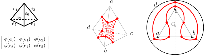
Figure 3: Left: Intersection symbol. Right: Tetrahedron with a polygonal cycle formed by $8$ normal arcs, bounding an octagon within the interior of the tetrahedron. Equivalent representation of the cycle as a loop in the disk with punctures $\{a,b,c\}$, and $d$ sent to the boundary. The loop in $\mathbb{D}_{3}$ is reduced, and has intersection symbol $[2\ \ 1\ \ 1]$.

3.1 Topology of the punctured disk

A homeomorphism $\mathbb{X}\to\mathbb{Y}$ between two topological spaces is a continuous bijective map with continuous inverse. Two topological spaces admitting a homeomorphism are said to be homeomorphic or topologically equivalent, and we write $\mathbb{X}\cong\mathbb{Y}$. Two homeomorphisms $f,g\colon\mathbb{X}\to\mathbb{X}$ from a closed topological space to itself are isotopic if there exists a continuous map $H:\mathbb{X}\times[0;1]\to\mathbb{X}$ satisfying $H(\cdot,0)=f$ and $H(\cdot,1)=g$, and for each $t\in[0;1]$, $H(\cdot,t)\colon\mathbb{X}\to\mathbb{X}$ is a homeomorphism.

Let $\mathbb{D}$ be the closed $2$-dimensional disk, and let $a,b,c\in\mathbb{D}$ be three distinct, arbitrary but fixed, points in its interior $\mathring{\mathbb{D}}=\mathbb{D}\setminus\partial\mathbb{D}$. Denote by $\mathbb{D}_{3}$ the $3$-punctured disk $\mathbb{D}\setminus\{a,b,c\}$. A self-homeomorphism $f\colon\mathbb{D}\setminus\{a,b,c\}\to\mathbb{D}\setminus\{a,b,c\}$ is isotopic to the identity if its completion $\widetilde{f}\colon\mathbb{D}\to\mathbb{D}$ is isotopic to $\mathrm{id}_{\mathbb{D}}$, by an isotopy $H\colon\mathbb{D}\times[0;1]\to\mathbb{D}$ that fixes points $a$, $b$ and $c$.

Let $\mathrm{Homeo}(\mathbb{D}_{3},\partial\mathbb{D})$ be the group, under composition, of (orientation preserving) homeomorphisms $\mathbb{D}_{3}\to\mathbb{D}_{3}$ that are the identity on the outer boundary $\partial\mathbb{D}$, and let $\mathrm{Homeo}_{0}(\mathbb{D}_{3},\partial\mathbb{D})$ be the subgroup of such homeomorphisms that are isotopic to the identity. We define the mapping class group of $\mathbb{D}_{3}$ relative to $\partial\mathbb{D}$ to be the group quotient:

$$\mathcal{MCG}(\mathbb{D}_{3},\partial\mathbb{D})=\mathrm{Homeo}(\mathbb{D}_{3},\partial\mathbb{D})/\mathrm{Homeo}_{0}(\mathbb{D}_{3},\partial\mathbb{D})$$

that we denote by $\mathcal{MCG}_{3}$ for short. It is known that $\mathcal{MCG}_{3}$ is isomorphic to the braid group $B_{3}$ [2]. This is the non-abelian group generated by two elements $\sigma_{1}$ and $\sigma_{2}$, satisfying $\sigma_{1}\sigma_{2}\sigma_{1}=\sigma_{2}\sigma_{1}\sigma_{2}$.

A free loop on $\mathbb{D}\setminus\{a,b,c\}$ is a continuous embedding of the circle $S^{1}$ into $\mathring{\mathbb{D}}\setminus\{a,b,c\}$, i.e. $L\colon S^{1}\to\mathbb{D}\setminus\{a,b,c\}$. A free loop is simple if it has no self intersection. Two simple free loops $L_{1},L_{2}$ are isotopic if there exists a self-homeomorphism of $\mathbb{D}\setminus\{a,b,c\}$ isotopic to the identity that sends the image of $L_{1}$ to the image of $L_{2}$. Recall that, due to the Jordan-Schoenflies theorem [2], a simple free loop in the plane separates the plane into two regions, the inside and the outside, and there exists a self-homeomorphism of the plane under which the loop is mapped onto the unit circle. We use the term loop to denote simple free loops as well as their image in $\mathbb{D}\setminus\{a,b,c\}$ as simple closed curves. Furthermore, we assume that all loops are smooth, and cut tetrahedron edges transversally. We refer to [2] for more details about these definitions.

3.2 Classification of loops by their intersection symbol

Given a tetrahedron $t$, its boundary $\partial t$ is a topological $2$-sphere. Removing each vertex of $t$, seen as a point, leads to the $4$-punctured sphere, or equivalently the $3$-punctured disk $\mathbb{D}_{3}$ (after closing the outer boundary). We also embed the tetrahedron edges in $\mathbb{D}_{3}$, as illustrated in Figure 3, using straight line segments. We say that a loop in $\mathbb{D}_{3}$ is reduced if it does not cross a tetrahedron edge twice in a row. We define the intersection symbol of a reduced loop in $\mathbb{D}_{3}$ to be the $2\times 3$ integer matrix of intersection numbers of the reduced loop with the tetrahedron edges embedded in $\mathbb{D}_{3}$. Note that reduced loops are the topological equivalent of the combinatorial “polygonal cycles” defined in Theorem 3.1 (by convention, we put the crossing numbers of edges $ab$, $bc$ then $bd$ in the first row of intersection symbols). Naturally, the intersection symbol of a reduced loop constitutes a valid tetrahedron intersection symbol. For a loop $L$ in $\mathbb{D}_{3}$, we denote its isotopy class by $[L]$; it is the class of all loops isotopic to $L$ in $\mathbb{D}_{3}$. We prove that the “intersection symbol” is well-defined for isotopy classes of loops.

Lemma 1

The following is true:

1. any isotopy class of loops in $\mathbb{D}_{3}$ admits a reduced loop,

2. any two isotopic reduced loops have equal intersection symbols,

3. any two non-isotopic reduced loops have distinct intersection symbols.

Proof

(i) Let $L$ be an arbitrary free loop. If $L$ is reduced, then $[L]$ contains a reduced free loop. Otherwise, $L$ crosses the same edge twice in a row. In this case we can deform $L$ locally via an isotopy, reducing the number of intersections between $L$ and the tetrahedron edges by two. Reproducing this deformation eventually leads to a reduced loop $L^{\prime}\in[L]$.

(ii) Let $\pi_{1}(\mathbb{D}_{3},\mathcal{O})$ be the fundamental group of the $3$-punctured disk with base point being the center of the triangle $\mathcal{O}$, see Figure 3. It is a classic result in planar topology (see for example [2]) that this group is the free non-abelian group with $3$ generators. Fixing an orientation, each of these generators is the homotopy class of the loop going around exactly one of the punctures exactly once—with the proper orientation. Equivalently, a generator is a loop that passes through exactly one of the segments $ad$, $bd$ and $cd$ in Figure 3 once—in the proper direction. Denote these generators by $\ell_{a}$, $\ell_{b}$ and $\ell_{c}$.

Let $L_{1}$ and $L_{2}$ be two isotopic, reduced, simple free loops. Fix points $x_{1}$ on $L_{1}$ and $x_{2}$ on $L_{2}$. Their intersection patterns with the line segments in $\mathbb{D}_{3}$, read starting from $x_{1}$ and $x_{2}$ respectively, define two words in $\pi_{1}(\mathbb{D}_{3})=\langle\ell_{a},\ell_{b},\ell_{c}\rangle$, denoted by $l_{1}$ and $l_{2}$ respectively. It is known (see for example [10]) that, for $L_{1}$ and $L_{2}$ isotopic free loops, $l_{1}$ and $l_{2}$ must be conjugate, i.e. there exists a word $w$ such that $l_{1}=wl_{2}w^{-1}$. Thus we can choose a new base-point $x^{\prime}_{1}$ on $L_{1}$ giving rise to $l^{\prime}_{1}=w^{-1}wl_{2}$, but $L_{1}$ was reduced, and thus $w$ must be empty, $l^{\prime}_{1}=l_{2}$, and $L_{1}$ and $L_{2}$ must have equal intersection symbols.

(iii) Suppose that two reduced loops $L_{1},L_{2}$ have same intersection symbol $s$. Using the construction from Theorem 3.1, we draw a “canonicial reduced loop” $L$ for the admissible symbol $s$, by fixing points on tetrahedron edges for each intersection described in $s$, and drawing the unique system of normal arcs to get $L\subset\mathbb{D}_{3}$. Because $L_{1}$ and $L_{2}$ are reduced, the restriction of $L_{1}$ (or $L_{2}$) to any triangular face (defined by the tetrahedron edges) is isotopic to the restriction of $L$ on this face. Since the intersection points on the triangular boundaries have to align, the isotopy can be made global, and both $L_{1}$ and $L_{2}$ are isotopic to $L$, hence $L_{1}$ and $L_{2}$ are isotopic. ∎

It follows that we can refer to the intersection symbol of an isotopy class of loops $[L]$ as the intersection symbol of any reduced loop in $[L]$. By a small abuse of notation, we also refer to the intersection symbol of a loop $L$ as the intersection symbol of $[L]$.

By virtue of the Jordan-Schoenflies theorem, we distinguish three types of loops: (i) loops containing no puncture in the inside; (ii) loops separating one puncture from the three others; and (iii) loops separating two punctures from the two others. Note that here we call the outer boundary of $\mathbb{D}_{3}$ “puncture” as well. Naturally, loops of type (i) are trivial and have intersection symbol $[0\ \ 0\ \ 0]$, and loops of type (ii) can be isotoped to a circle in a small neighbourhood of the puncture in their inside, and hence have $(2\times 3)$-intersection symbol $\left[\begin{array}[]{lll}1&0&1\\ 0&1&0\end{array}\right]$, up to tetrahedron permutations. The case of loops of type (iii) is more interesting; we call these loops balanced. We prove:

Lemma 2

For any two loops $L_{1}$ and $L_{2}$ of same type (i), (ii) or (iii), there exists a homeomorphism of $\mathbb{D}_{3}$, constant on $\partial\mathbb{D}$, sending $L_{1}$ to $L_{2}$.

Proof

This is a consequence of the Jordan-Schoenflies theorem. Consider the completion of $\mathbb{D}_{3}=\mathbb{D}\setminus\{a,b,c\}$ into $\mathbb{D}$ by filling up the three punctures. Let $h_{1}\colon\mathbb{D}\to\mathbb{D}$ and $h_{2}\colon\mathbb{D}\to\mathbb{D}$ be two self-homeomorphisms of the plane sending $L_{1}$ and $L_{2}$, respectively, to the unit circle. Consequently, $h_{2}^{-1}\circ h_{1}$ is a self-homeomorphism of $\mathbb{D}$ sending $L_{1}$ to $L_{2}$. Since $L_{1}$ and $L_{2}$ are of the same type, their inside and outside in $\mathbb{D}\setminus\{a,b,c\}$ are homeomorphic, by a homeomorphism that preserves the boundary $L_{2}\cup\partial\mathbb{D}$ (this homeomorphism “aligns” punctures). Composing $h_{2}^{-1}\circ h_{1}$ with this homeomorphism sends $\{a,b,c\}$ to $\{a,b,c\}$ in $\mathbb{D}$, and defines the self-homeomorphism of $\mathbb{D}_{3}$ sending $L_{1}$ to $L_{2}$. ∎

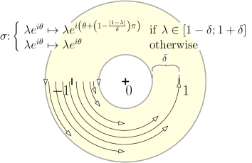
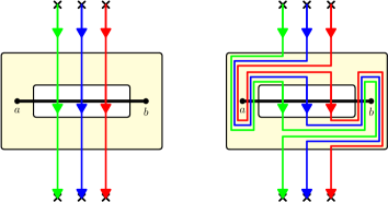
Figure 4: Left: Construction of a homeomorphism in the complex plane exchanging $-1$ with $1$ (in the positive direction) as a model to exchange positions of punctures $a$ and $b$ in $\mathbb{D}_{3}$. Right: Action of the homeomorphism exchanging punctures at $a$ and $b$ on pieces of loop crossing edge $ab$ transversally (the annulus has been placed in a close neighbourhood of edge $ab$, with $-1$ on puncture $a$ and $1$ on puncture $b$). Note that the curves must cross the annulus and edge $ab$ transversally; to maintain this property, we assume that we deform isotopically the loops “outside” the annulus after applying the homeomorphism.

As a consequence, intersection symbols of loops are defined up to isotopy with the identity, and any pair of loops are related by a homeomorphism. Hence, the action of an element (i.e. a class of homeomorphisms) of the mapping class group $\mathcal{MCG}_{3}$ on an intersection symbol is well defined. Before classifying balanced loops, we give an explicit characterisation of the generators of the mapping class group $\mathcal{MCG}_{3}$, coming from the isomorphism with the braid group $B_{3}$. These generators are classes of homeomorphisms, exchanging two punctures. See Figure 4 for an explicit homeomorphism exchanging punctures $a$ and $b$, and its local action on curves intersecting the line segment $ab$ transversally. The homeomorphism is the identity everywhere except for in a small annulus containing $a$ and $b$. Denote by $\sigma_{ab}$ and $\sigma_{bc}$ the homeomorphisms, as defined in Figure 4, exchanging punctures $a$ with $b$, and punctures $b$ with $c$ respectively. We now classify the intersection symbols of balanced loops.

Theorem 3.2

There is a bijection between isotopy classes of balanced loops in $\mathbb{D}_{3}$ and intersection symbols of the form $[i\ \ j\ \ i+j]$, up to tetrahedron permutation, with $i$, $j$ coprime non-negative integers.

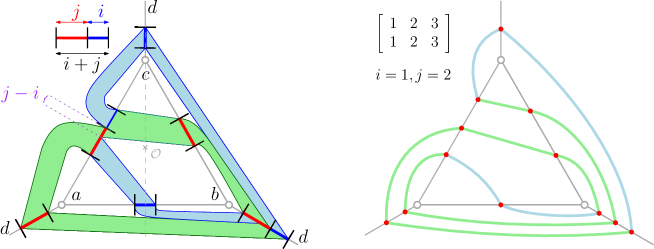
Figure 5: Reduced loop, given by the intersection symbol $[i\ \ j\ \ i+j]$ with $j\geq i$. Blue domains represent $i$ parallel segments and green domains represent $j$ parallel segments. Note in particular that the $j$ segments, in the green domain inside the central triangle, originating from edge $bc$ and crossing edge $ac$, split into $j-i$ segments crossing $ad$ and $i$ segments crossing $cd$. The center $\mathcal{O}$ and vertical axis are drawn in grey.

Proof

Recall that we denote intersection symbols with two identical rows only by their first row $[i\ \ j\ \ i+j]$ and, by symmetry, we suppose $j\geq i$. The proof is separated into two parts (i) (intersection symbol equals $[i\ \ j\ \ i+j]$) and (ii) ($i$ and $j$ are coprime).

(i) We first prove that balanced loops have intersection symbols $[i\ \ j\ \ i+j]$, up to permutation, for arbitrary $i,j\geq 0$. By virtue of Lemma 2, any balanced loop $L$ in $\mathbb{D}_{3}$ may be obtained via a homeomorphism $h\colon\mathbb{D}_{3}\to\mathbb{D}_{3}$ from the reduced loop $L_{0}$ with intersection symbol $[0\ \ 1\ \ 1]$. By virtue of the isomorphism $\mathcal{MCG}_{3}\cong B_{3}$, this homeomorphism $h$ can be expressed as $g\circ f$, where $f$ is a composition of the homeomorphisms $\sigma_{ab}$ and $\sigma_{bc}$, and $g$ is isotopic to the identity. Because intersection symbols are defined up to isotopy with the identity, we focus on the action of the homeomorphisms $\sigma_{ab}$ and $\sigma_{bc}$ on the intersection symbol of an (balanced) loop. Recall that $\sigma_{ab}$ and $\sigma_{bc}$ are homeomorphisms that exchange punctures $a$ with $b$, and puncture $b$ with $c$ respectively, in the positive direction. We specify the homeomorphism $\sigma_{ab}$ exactly in Figure 4 and show its action on curves intersecting edge $ab$ transversally. Note that these homeomorphisms are similar to Dehn twists in the study of surface topology.

We prove the result inductively. The intersection symbol of the base case $L_{0}$ satisfies the property with $i=0$ and $j=1$. Suppose that we are given a reduced loop $L$ in $\mathbb{D}_{3}$ with intersection symbol $[i\ \ j\ \ i+j]$. Figure 5 represents such loop. We study the action of $\sigma_{ab}$ and $\sigma_{bc}$ on the intersection symbol of such a loop.

All tetrahedron permutations may be obtained by rotations of $2\pi/3$ around center $\mathcal{O}$ and reflections along the vertical axis passing through puncture $c$; see Figure 5. In order to reduce the study to a limited number of cases, note that exchanging any two punctures is equivalent to applying the appropriate rotation, exchanging the bottom two punctures and rotating back to the original position. Hence we study only the action of $\sigma_{ab}$ and $\sigma_{ab}^{-1}$. Additionally, applying $\sigma_{ab}$ to a loop $L$ or $\sigma_{ab}^{-1}$ to its reflection $L^{\prime}$ along the vertical axis, is equivalent; specifically, denoting by $X$ a configuration and by $\overline{X}$ its reflection along the vertical axis, we have $\sigma_{ab}(\overline{X})=\overline{\sigma_{ab}^{-1}(X)}$. For simplicity we denote $\sigma_{ab}$ by $\sigma$ for the remainder of this proof.

Figure 7 shows a detailed example of the action of $\sigma$ on a piece of loop traversing $ab$ transversally. Figure 6 pictures all possible cases of a piece of loop intersecting edge $ab$, together with a neighbourhood of the intersection. These configurations and their reflected versions appear on one of the edges $\{ab,bc,ac\}$ in Figure 5, picturing the the loop with intersection symbol $[i\ \ j\ \ i+j]$ of the inductive argument. The action of $\sigma$ and $\sigma^{-1}$ is local in the sense that only a piece of the loop in a neighbourhood of the intersection with the edge $ab$ needs to be considered to reduce the loop after transformation. Additionally, the five configurations $A,O_{1},O_{2},O_{3}$ and $O_{4}$ of Figure 6 can be regarded independently, because the considered neighbourhoods do not overlap. Finally, the modification of the intersection symbol induced by the homeomorphisms $\sigma$ and $\sigma^{-1}$ on a single piece of loop is pictured by $2\times 3$-matrices in Figure 6.

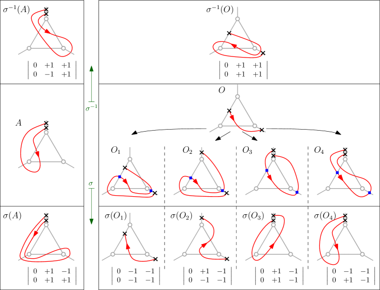
Figure 6: Pieces of loop traversing edge $ab$. We distinguish two cases: case $A$ where the loop originates from edge $ac$, crosses $ab$ then $ad$, and case $O$ where the loop originates from edge $ac$, crosses $ab$ then $bd$. For the action of $\sigma$, we distinguish $4$ subcases $O_{1}$ to $O_{4}$ to case $O$, as the loop gets shortened by isotopy in order to maintain the property of being reduced (the original piece $O$ is delimited by blue squares in special cases $O_{1}$ to $O_{4}$). The black crosses represent fixed points for the action of $\sigma$, $\sigma^{-1}$ and the isotopy reduction; in particular, the loop is reduced when the piece between the black crosses does not cross twice the same edge, and the piece of loop enters or leave a fixed point with the same orientation. The loop pieces $\{A,O_{1},O_{2},O_{3},O_{4}\}$ and their reflections cover all possible crossing configurations found on an edge $\{ab,bc,ac\}$ of a loop with intersection symbol $[i\ \ j\ \ i+j]$ as in Figure 5.

We apply the homeomorphisms $\sigma$ and $\sigma^{-1}$ to all three $2\pi/3$ rotations of the intersection symbol $[i\ \ j\ \ i+j]$ and express the transformation in terms of the matrices presented in Figure 6. Due to the independence of configurations $A,O_{1},O_{2},O_{3},O_{4}$, we can linearly sum the $2\times 3$ matrices for all pieces of loop intersecting edge $ab$. Below we list all crossing configurations with edge $ab$ for all permutations of the intersection symbol; the transformation of the intersection symbol can be calculated in the following way:

$$\begin{array}[]{lcll}[i\ \ j\ \ i+j]&\equiv&i\times O_{1}&\left\{\begin{array}[]{cl}\xmapsto{\ \ \sigma\ \ }&[i\ \ j-i\ \ j]\\ \xmapsto{\ \sigma^{-1}}&[i\ \ i+j\ \ 2i+j]\\ \end{array}\right.\\ &&&\\ [i+j\ \ i\ \ j]&\equiv&i\times(A+\overline{A})+(j-i)\times O_{3}&\left\{\begin{array}[]{cl}\xmapsto{\ \ \sigma\ \ }&[i+j\ \ 2i+j\ \ i]\\ \xmapsto{\ \sigma^{-1}}&[i+j\ \ j\ \ i+2j]\\ \end{array}\right.\\ &&&\\ [j\ \ i+j\ \ i]&\equiv&\begin{array}[]{ll}\max(0,2i-j)\times\overline{O_{1}}+\max(0,j-2i)\times\overline{O_{3}}\\ +\min(i,j-i)\times(\overline{O_{2}}+\overline{O_{4}})\\ \end{array}&\left\{\begin{array}[]{cl}\xmapsto{\ \ \sigma\ \ }&[j\ \ i+2j\ \ i+j]\\ \xmapsto{\ \sigma^{-1}}&[j\ \ i\ \ j-i]\\ \end{array}\right.\\ \end{array}$$

Note that the more intricate case study ($j>2i$ or not) of the case $[j\ \ i+j\ \ i]$ is due to pieces of loop intersecting edges with a “split” twice in the neighbourhood considered, explaining the $2^{2}=4$ subcases (see the “split” intersection patterns on edges $bd$ and $ac$ in Figure 5). In summary, applying $\sigma$ preserves the fact that the intersection symbol is of the form $[i\ \ j\ \ i+j]$, up to permutation.

(ii) We now prove that $i$ and $j$ are coprime integers. Note that we can simulate the Euclidean algorithm on the pair $(j,i)$ by applying $\sigma$. W.l.o.g., consider the intersection symbol $[i\ \ j\ \ i+j]$, $j\geq i$. Note that, if $j>1$ then $j>i$: assuming otherwise $i=j>1$, then applying $\sigma$ induces the symbol $[i\ \ 0\ \ i]$ which represents multiple parallel disjoint copies of the loop $[1\ \ 0\ \ 1]$. Consider the division $j=qi+r$, with $r<i$. Applying $\sigma$ $q$ times to $[i\ \ j\ \ i+j]$ gives $[i\ \ r\ \ i+r]$ with $r<i$. Hence we can recursively apply the Euclidean algorithm on the pair $(i,r)$. Because of the property that $j\neq i$, the algorithm terminates on the pair $(1,0)$ and $\gcd(i,j)=1$. Conversely, for any coprime integers $(p,q)$, running the Euclidean algorithm in reverse gives us the sequence of homeomorphisms $\sigma_{ab}$, $\sigma_{bc}$, and their inverses to obtain the loop $[p\ \ q\ \ p+q]$ from the loop $[0\ \ 1\ \ 1]$.

The bijection now follows by virtue of Lemma 1. ∎

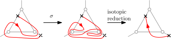
Figure 7: Action of $\sigma_{ab}$, with isotopic reduction, on a piece of loop and its neighbourhood (we call this loop configuration $O_{1}$).

Theorem 3.3

An admissible tetrahedron colouring corresponds to a family of polygonal curves with intersection symbols

$$a\times\left[\begin{array}[]{ccc}1&0&1\\ 0&1&0\\ \end{array}\right]+b\times\left[\begin{array}[]{ccc}1&1&0\\ 0&0&1\\ \end{array}\right]+c\times\left[\begin{array}[]{ccc}0&1&1\\ 1&0&0\\ \end{array}\right]+d\times\left[\begin{array}[]{ccc}0&0&0\\ 1&1&1\\ \end{array}\right]$$

for arbitrary integers $a,b,c,d\geq 0$, and $p\geq 0$ copies of the same polygonal curve with intersection symbol

$$\left[\begin{array}[]{ccc}i&j&i+j\\ i&j&i+j\\ \end{array}\right]\ \text{or}\ \left[\begin{array}[]{ccc}i+j&i&j\\ i+j&i&j\\ \end{array}\right]\ \text{or}\ \left[\begin{array}[]{ccc}j&i+j&i\\ j&i+j&i\\ \end{array}\right]$$

for arbitrary coprime integers $i,j\geq 0$, not both $0$. Integers $a,b,c,d,p,i,j$ are defined such that the bound $r-2$ on edge colourings is respected.

Proof

The seven intersection symbols are exactly the ones of the isotopy classes of loops in $\mathbb{D}_{3}$, and hence exactly the ones of all possible polygonal curves on the boundary of a tetrahedron (Theorem 3.2). In $\mathbb{D}_{3}$, we can draw an arbitrary number of loops separating one puncture from the three others, by drawing them in a close neighbourhood of the puncture they isolate. These loops are exactly the ones with one of the four first intersection symbols of the theorem.

We prove that a tetrahedron $t$ can have only one type of polygonal cycle with one of the three last intersection symbols of the theorem. Take two such polygonal loops; by definition, they are disjoint on $\partial t$. Let $L_{1}$ and $L_{2}$ be the corresponding two pairwise disjoint loops in $\mathbb{D}_{3}$; they are balanced by definition. Because they are disjoint, suppose, w.l.o.g., that $L_{2}$ is contained in the inside of $L_{1}$. As $L_{1}$ and $L_{2}$ both contain two punctures in their inside, the “band” between $L_{1}$ and $L_{2}$ (i.e. the inside of $L_{1}$ minus the inside of $L_{2}$) contains no puncture, and is then a topological annulus, with boundary $L_{1}\sqcup L_{2}$. Sliding $L_{2}$ along the annulus gives an isotopy between $L_{1}$ and $L_{2}$ that is constant outside (a neighbourhood of) the annulus, and in particular fixes the punctures. Consequently, $L_{1}$ and $L_{2}$ have same intersection symbol (Lemma 1(ii)). Conversely, given an balanced loop $L$, an arbitrary number of loops with same intersection symbol can be drawn in a neighbourhood of $L$. ∎

In conclusion, Theorem 3.3 gives an explicit characterisation of admissible tetrahedron colourings in terms of polygonal cycles. We use this “system of coordinates” to re-write the formulae for the weights of the tetrahedra as defined in Section 2.4 for the Turaev-Viro invariant at $sl_{2}(\mathbb{C})$. Namely, we have the following observation.

Theorem 3.4

Let $t=\{a,b,c,d\}$ be a tetrahedron, coloured as in Theorem 3.3, i.e. with $a$ (respectively $b$, $c$ and $d$) copies of a $3$-cycle around vertex $a$ (respectively, around vertices $b$, $c$ and $d$), and $p$ copies of the balanced loop $[i\ \ j\ \ i+j]$. Then, we can express the weight of $t$ as

$$|t|=(-1)^{X}\sum_{0\leq z\leq d}\frac{(-1)^{z}[X-z+1]!}{[a-z]![b-z]![c-z]![d-z]![pi+z]![pj+z]![z]!},$$

where $X:=p(i+j)+a+b+c+d$ and $y:=\min\{a,b,c,d\}$, and, if $y=0$,

$$|t|=\frac{[X+1]!}{[a]!\ [b]!\ [c]!\ [d]!\ [pi]!\ [pj]!}.$$

Proof

The proof consists of an explicit calculation. Given a coloured tetrahedron $t$ with intersection symbol as in Figure 8. Denote its set of colours by $\Phi$. Note that the “edge colours” on the picture are integers—as in the definition of the intersection symbol—and must be divided by two to fit the definition of the Turaev-Viro invariant in Section 2.4, using half-integers.

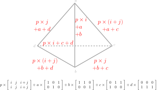
Figure 8: Colouring a tetrahedron using the coordinate system of Theorem 3.3.

In Section 2.4, $z^{-}$ and $z^{+}$ are defined as the maximum values of the sum of edge colours of a triangular face, and the minimum values of the sum of the edge colours of a quad (i.e., all edges but two opposite ones). Summing the colours, divided by two yields

$$\text{Triangles}:\ \left\{\begin{array}[]{l}p\times(i+j)+a+b+c\\ p\times(i+j)+a+b+d\\ p\times(i+j)+a+c+d\\ p\times(i+j)+b+c+d\\ \end{array}\right.\ \ \text{Quads}:\ \left\{\begin{array}[]{l}p\times(i+j)+p\times j+a+b+c+d\\ p\times(i+j)+p\times i+a+b+c+d\\ p\times(i+j)+a+b+c+d.\\ \end{array}\right.$$

Let $y:=\min\{a,b,c,d\}$. Consequently, $z^{-}=p\times(i+j)+a+b+c+d-y$ and $z^{+}=p\times(i+j)+a+b+c+d$. Replacing the variable $z$, in the definition of a tetrahedron weight in Section 2.4, by $z-z^{-}$ we obtain

$$|t|_{\Phi}=\sum_{0\leq z\leq y}\frac{(-1)^{p\times(i+j)+a+b+c+d}\times(-1)^{z-y}[z+(p\times(i+j)+a+b+c+d-y)+1]!}{[z+a-y]![z+b-y]![z+c-y]![z+d-y]!\times[y+pi-z]![y+pj-z]![y-z]!};$$

and introducing $X:=p\times(i+j)+a+b+c+d$, and substituting $z$ by $y-z$ results in

$$|t|_{\Phi}=(-1)^{X}\sum_{0\leq z\leq y}\frac{(-1)^{z}[X-z+1]!}{[a-z]![b-z]![c-z]![d-z]!\times[pi+z]![pj+z]![z]!}.$$

∎

3.3 Admissible colourings as embedded surfaces

In this section, we give a more intuitive and topological understanding of admissible colourings in terms of embedded surfaces within the triangulation. By interpreting the polygonal cycles as intersection patterns of these embedded surfaces with the boundary $\partial t$ of the tetrahedron $t$, an admissible colouring can be seen as a family of embedded surfaces.

This approach is a powerful tool in computational topology of $3$-manifolds. It is in particular of key importance in the unknot recognition algorithm [9]—using normal surfaces—and in the $3$-sphere recognition algorithm [18]—using almost normal surfaces. Normal surfaces consider embedded surfaces cutting through $\partial t$ with $3$-gons, and $4$-gons $[0\ \ 1\ \ 1]$. Almost normal surfaces allow, in addition, $8$-gons $[1\ \ 1\ \ 2]$. Theorem 3.3 states that Turaev-Viro invariants, for $r$ sufficiently large, consist of formulae involving weights defined on much more complicated surface pieces, with intersection symbol $[i\ \ j\ \ i+j]$. These intersections are “helicoidal” surface pieces of higher index; see [1] for a recent study on embedded surfaces containing these pieces.

The efficient algorithm for computing the Turaev-Viro invariant for $r=3$ is based on a relation between $\mathrm{TV}_{3}$ and $2$-homology, and can be interpreted in terms of embedded surfaces. A generalisation of this idea to design more efficient algorithms for arbitrary $r>3$, using the classification of embedded surface pieces from this section, is subject of ongoing research.

4 Bounds on the number of admissible colourings

Given a $3$-manifold triangulation $\mathfrak{T}$ with $v$ vertices, $n+v$ edges, $2n$ triangles and $n$ tetrahedra (the relations between number of faces follows from an Euler characteristic argument), and following the definitions in Section 2.2 above, there are at most $(r-1)^{n+v}$ admissible colourings for $\mathrm{TV}_{r,q}$. This bound is usually far from being sharp. However, current enumeration algorithms for admissible colourings do not try to capitalise on this fact in a controlled fashion.

In this section we discuss improved upper bounds on the number of admissible colourings in important special cases. Moreover, we give a number of examples where these improved bounds are actually attained. The bounds are used in Section 5 to construct a significant exponential speed-up for the computation of $\mathrm{TV}_{r,1}$ where $r$ is odd.

Note that in the following, we go back to the convention of using half-integers for the colourings of edges.

4.1 Vertices and the first Betti number

First let us have a look at some triangulations where we can a priori expect a rather large number of colourings.

Proposition 2

Let $\mathfrak{T}$ be a $3$-manifold triangulation with $v$ vertices. Then

$$|\mathrm{Adm}(\mathfrak{T},3)|=2^{v+\beta_{1}(\mathfrak{T},\mathbb{Z}_{2})-1}.$$

Proof

Every colouring $\theta\in\mathrm{Adm}(\mathfrak{T},3)$ can be associated to a $1$-cocycle $c_{\theta}$ of $\mathfrak{T}$ over the field with two elements $\mathbb{Z}_{2}$: Simply define $c$ to be the $1$-cocycle evaluating to $c(e)=1$ on edges coloured $\theta(e)=1/2$, and to $c(e)=0$ on edges coloured $\theta(e)=0$. Conversely, every $1$-cocycle $c$ defines an admissible colouring $\theta_{c}\in\mathrm{Adm}(\mathfrak{T},3)$. By construction two admissible colourings are distinct if and only if their associated $1$-cocycles are distinct. Hence, the number of admissible colourings $|\mathrm{Adm}(\mathfrak{T},3)|$ must equal the number of $1$-cocycles of $\mathfrak{T}$.

First of all $\mathfrak{T}$ has $2^{\beta_{1}(\mathfrak{T},\mathbb{Z}_{2})}$ $1$-cohomology classes. Moreover for every $1$-cocycle $c$ we can find a homologous—but distinct—$1$-cocycle $c^{\prime}$ by adding a non-zero $1$-coboundary to $c$. The statement now follows by noting that the number of $1$-coboundaries of any triangulation $\mathfrak{T}$ equals the number of subsets of vertices of even cardinality, which is $2^{v-1}$. ∎

$n$	$\#$ trigs.	$\#$ sharp (3)
$1$	$1$	$1$
$2$	$4$	$1$
$3$	$24$	$4$
$4$	$160$	$4$
$5$	$1492$	$14$
$6$	$16731$	$22$

Table 1: Number “$\#$ trigs.” of $1$-vertex triangulations $\mathfrak{T}$ of manifolds with $\beta_{1}(\mathfrak{T},\mathbb{Z}_{2})=1$ and $n$ tetrahedra, $1\leq n\leq 6$, and number of cases of equality “$\#$ sharp (3)” in the bound from Theorem 4.1.

Proposition 2 is a basic but very useful observation with consequences for $\mathrm{Adm}(\mathfrak{T},4)$. This is particularly exiting as computing $\mathrm{TV}_{4,1}$ is known to be $\#P$-hard. More precisely, the following statement holds.

Theorem 4.1

Let $\mathfrak{T}$ be an $n$-tetrahedron $3$-manifold triangulation with $v$ vertices, and let $\theta\in\mathrm{Adm}(\mathfrak{T},3)$. Furthermore, let $\ker_{\theta}$ be the number of edges coloured $0$ by $\theta$. Then

$$|\mathrm{Adm}(\mathfrak{T},4)| \leq\left(\Sigma_{\theta\in\mathrm{Adm}(\mathfrak{T},3)\setminus\{{\bf 0}\}}2^{\ker_{\theta}}\right)+2^{v+\beta_{1}(\mathfrak{T},\mathbb{Z}_{2})-1}$$ (2)

$$\leq(|\mathrm{Adm}(\mathfrak{T},3)|-1)(2^{n+v-1}+1)+1,$$ (3)

where $\mathbf{0}$ denotes the zero colouring. Moreover, both bounds are sharp.

Proof

Let $\theta\in\mathrm{Adm}(\mathfrak{T},4)$, and let $\theta^{\prime}$ be its reduction, as defined in Proposition 1. If $\theta^{\prime}$ is the trivial colouring (that is, if no colour of $\theta$ is coloured by $1/2$) the colouring $\theta/2$, obtained by dividing all of the colours of $\theta$ by two, must be in $\mathrm{Adm}(\mathfrak{T},3)$. It follows from Proposition 2 that exactly $2^{v+\beta_{1}(\mathfrak{T},\mathbb{Z}_{2})-1}$ colourings in $\mathrm{Adm}(\mathfrak{T},4)$ reduce to the trivial colouring.

If $\theta^{\prime}$ is not the trivial colouring then $\theta$ colours some edges by $1/2$. In particular it is not the trivial colouring. Since the only colours in $\theta$ are $0$, $1/2$, and $1$, all edges coloured by $1/2$ in $\theta$ are coloured by $1/2$ in $\theta^{\prime}$ and vice versa. Thus, $\ker_{\theta^{\prime}}$ denotes all edges coloured by $0$ or $1$ in $\theta$. Naturally, there are at most $2^{\ker_{\theta^{\prime}}}$ such colourings. The result now follows by adding these upper bounds $2^{\ker_{\theta^{\prime}}}$ over all non-trivial reductions $\theta^{\prime}\in\mathrm{Adm}(\mathfrak{T},3)$, and adding the $2^{v+\beta_{1}(\mathfrak{T},\mathbb{Z}_{2})-1}$ extra colourings with trivial reduction.

Equation (3) follows from the fact that in every non-trivial colouring in $\mathrm{Adm}(\mathfrak{T},3)$ there must be at least one edge coloured $1/2$ and thus $\ker_{\theta^{\prime}}$ can be at most the number of edges minus one.

It follows that for $\beta_{1}(\mathfrak{T},\mathbb{Z}_{2})$ or $v$ sufficiently large this bound cannot be tight. For $1$-vertex $\mathbb{Z}_{2}$-homology spheres this bound is sharp as explained in Corollary 1 below. Looking at all $1$-vertex triangulations with $\beta_{1}(\mathfrak{T},\mathbb{Z}_{2})=1$ up to six tetrahedra, the cases of equality in Inequality (3) are summarised in Table 1. See Table 2 for a large number of cases of equality for Inequality (2). ∎

$(n,\beta_{1})$	$\#$ trig.	$\#$ sharp (2)	$(r-1)^{n+v}$	$\#$ tree	Eqn. (3)	Eqn. (2)	$\overline{|\mathrm{Adm}(\mathfrak{T},4)|}$
$(1,1)$	$1$	$1$	$9$	$12.0$	$4$	$4$	$4$
$(2,1)$	$5$	$5$	$37.8$	$33.0$	$10.4$	$6.0$	$6.0$
$(2,2)$	$1$	$1$	$27.0$	$39.0$	$16.0$	$10.0$	$10.0$
$(3,1)$	$27$	$14$	$99.0$	$46.4$	$14.7$	$7.7$	$6.3$
$(3,2)$	$3$	$1$	$81.0$	$69.0$	$28.0$	$14.7$	$11.3$
$(4,1)$	$205$	$67$	$378.1$	$75.2$	$42.9$	$13.1$	$8.7$
$(4,2)$	$19$	$4$	$268.6$	$110.1$	$61.5$	$21.8$	$15.3$
$(5,1)$	$1858$	$261$	$1131.6$	$93.1$	$85.5$	$20.4$	$9.3$
$(5,2)$	$184$	$10$	$887.5$	$159.2$	$138.7$	$35.8$	$18.6$
$(6,1)$	$21459$	$1574$	$3644.8$	$120.4$	$195.3$	$34.6$	$10.7$
$(6,2)$	$2516$	$47$	$2781.6$	$214.5$	$297.5$	$58.0$	$22.0$
$(6,3)$	$34$	$0$	$2187.0$	$413.2$	$456.0$	$94.5$	$41.4$

Table 2: Analysis of the trivial bound “$(r-1)^{n+v}$” (fourth column), average number of nodes “$\#$ tree” of the search tree visited by the backtracking algorithm (fifth column), bound “Eqn. (3)” given by the Inequality (3) (sixth column), bound “Eqn. (2)” given by Inequality (2) (seventh column), and average number “$\overline{|\mathrm{Adm}(\mathfrak{T},4)|}$” of admissible colourings in $\mathrm{Adm}(\mathfrak{T},4)$ (rightmost column). The second column lists the number of triangulations “$\#$ trig.” contained in the census of triangulated closed manifolds $\mathfrak{T}$ with $n$ tetrahedra and first Betti number $\beta_{1}(\mathfrak{T},\mathbb{Z}_{2})$, the third column lists the number “$\#$ sharp (2)” of triangulations satisfying equality in Inequality (2).

Given a triangulation $\mathfrak{T}$, the right hand side of Equation (2) can be computed efficiently. It turns out to be sharp for $1985$ out of all $26,312$ closed triangulated $3$-manifolds with positive first Betti number and up to $6$ tetrahedra. In addition, even the average number of colourings is fairly close to this bound. See Table 2 for details comparing the first upper bound to the actual number of colourings in the census. Furthermore, there are $46$ triangulations of $3$-manifolds with $\leq 6$ tetrahedra (and positive first Betti number) attaining equality in the often much larger right hand side of Equation (3). For details about these cases of equality see Table 1.

We have seen that the number of colourings in $\mathrm{Adm}(\mathfrak{T},3)$ and $\mathrm{Adm}(\mathfrak{T},4)$ largely depend on (i) the number of tetrahedra, (ii) the number of vertices, and (iii) the first Betti number of $\mathfrak{T}$. Moreover, if $\theta\in\mathrm{Adm}(\mathfrak{T},r)$ then $\theta\in\mathrm{Adm}(\mathfrak{T},r^{\prime})$ for $r^{\prime}\geq r$, and colourings for a lower value of $r$ possibly give rise to an exponential number of colours for a higher value of $r$.

Hence, we can expect the number of admissible colourings in $1$-vertex $\mathbb{Z}_{2}$-homology spheres to be smaller than in the generic case. Incidentally, homology spheres are manifolds for which computing $\mathrm{TV}_{r,q}$ is of particular interest in view of $3$-sphere recognition. For this reason we have a closer look at this very important special case below.

4.2 One-vertex $\mathbb{Z}_{2}$-homology spheres

When talking about algorithms to compute $\mathrm{TV}_{r,q}(\mathfrak{T})$ for some $3$-manifold triangulation $\mathfrak{T}$, the case of $\mathbb{Z}_{2}$-homology spheres with only one vertex is a special case of particular importance for several reasons.

1. One of the most important tasks of $3$-manifold invariants is to distinguish between some $3$-manifold triangulation $\mathfrak{T}$ and the $3$-sphere. In many cases homology can be used to efficiently make this distinction. Hence, this question is most interesting when homology fails, that is, when $\mathfrak{T}$ is a homology sphere.

2. All results about $\mathrm{TV}_{r,q}$ which apply to $\mathbb{Z}_{2}$-homology spheres automatically carry through for the invariant $\mathrm{TV}_{r,1}(\mathfrak{T},[0])$ for arbitrary manifold triangulations $\mathfrak{T}$.

3. There are powerful techniques available to turn a triangulation of a $\mathbb{Z}_{2}$-homology sphere with an arbitrary number of vertices into a set of smaller triangulations, all with only one vertex, see Section 5 for details.

In this section we take a closer look at $1$-vertex $\mathbb{Z}_{2}$-homology spheres and in particular their number of admissible colourings. One corollary of Proposition 2 is the following statement for $\mathbb{Z}_{2}$-homology spheres.

Corollary 1

Let $\mathfrak{T}$ be a $1$-vertex $\mathbb{Z}_{2}$-homology sphere. Then $|\mathrm{Adm}(\mathfrak{T},r)|=1$ for $r\leq 4$.

Proof

For $r=3$ this is a direct consequence from Proposition 2, for $r=4$ this is a direct consequence from Theorem 4.1. ∎

In particular, $\mathbb{Z}_{2}$-homology spheres (including many lens spaces) can never be distinguished from the $3$-sphere by $\mathrm{TV}_{r,q}$, $r\leq 4$.

Proposition 3

Let $\mathfrak{T}$ be a $1$-vertex $n$-tetrahedron $\mathbb{Z}_{2}$-homology sphere. Then for all $\theta\in\mathrm{Adm}(\mathfrak{T},r)$, all colours of $\theta$ are integers, and in particular

$$|\mathrm{Adm}(\mathfrak{T},r)|\leq\left\lfloor\frac{r}{2}\right\rfloor^{n+1}.$$

Proof

It follows from Propositions 1 and 2 that no admissible colouring of $\mathfrak{T}$ can contain half-integers. Furthermore, the edge colours on every triangle must sum to at most $r-2$ and satisfy the triangle inequality. It follows that all colours must be integers between $0$ and $\lfloor\frac{r-2}{2}\rfloor$. The statement now follows from the fact that $\mathfrak{T}$ has $n+1$ edges. ∎

Corollary 2

Let $\mathfrak{T}$ be a $1$-vertex $n$-tetrahedron closed $3$-manifold triangulation. Then all admissible colourings to compute $\mathrm{TV}_{r,1}(\mathfrak{T},[0])$ contain integer weights only.

Proof

Let $\mathfrak{T}$ be a $1$-vertex triangulation. To compute $\mathrm{TV}_{r,1}(\mathfrak{T},[0])$ we only consider colourings $\theta$ with reductions $\theta^{\prime}$ corresponding to $1$-coboundaries ($1$-cocycles homologous to $0$). Because $\mathfrak{T}$ has only one vertex, $\theta^{\prime}$ must be the zero colouring and in particular no half-integers can occur in $\theta$. ∎

A similar statement for the case of special spines can be found in [15, Remark 8.1.2.2].

The bound from Proposition 3 cannot be sharp since not all triangle colourings $(a,b,c)\in\{0,1,\ldots,\lfloor\frac{r-2}{2}\rfloor\}^{3}$ are admissible. However, for $5\leq r\leq 7$ we have the following situation.

Theorem 4.2

Let $\mathfrak{T}$ be a $1$-vertex $n$-tetrahedron $\mathbb{Z}_{2}$-homology $3$-sphere triangulation, then

$$|\mathrm{Adm}(\mathfrak{T},5)|\leq 2^{n}+1;\quad\quad|\mathrm{Adm}(\mathfrak{T},6)|\leq 3^{n}+1;\quad\quad|\mathrm{Adm}(\mathfrak{T},7)|\leq 3^{n}+1.$$

Moreover, all these upper bounds are sharp.

Proof

For $r=5$ the admissible triangle colourings are $(0,0,0)$, $(1/2,1/2,0)$, $(1,1,0)$, $(1,1/2,1/2)$, $(1,1,1)$, $(3/2,3/2,0)$, $(3/2,1,1/2)$, up to permutations. By Proposition 1, no colouring in $\mathrm{Adm}(\mathfrak{T},5)$ can contain an edge colour $1/2$ or $3/2$. To see this note that otherwise the reduction of such a colouring would be a non-trivial colouring in $\mathrm{Adm}(\mathfrak{T},3)$, which does not exist (cf. Proposition 2 and Corollary 1 with $v=1$ and $\beta_{1}(\mathfrak{T},\mathbb{Z}_{2})=0$). Hence, all edge colours must be $0$ or $1$, leaving triangle colourings $(0,0,0)$, $(1,1,0)$, and $(1,1,1)$.

By an Euler characteristic argument, a $1$-vertex $n$-tetrahedron $3$-manifold has $n+1$ edges. Hence the number of colourings of $\mathrm{TV}_{5,q}$ is trivially bounded above by $2^{n+1}$. Furthermore, let $\theta\in\mathrm{Adm}(\mathfrak{T},5)$, then either $\theta$ is constant $0$ on the edges, constant $1$ on the edges, or $\theta$ contains a triangle coloured $(1,1,0)$. In the last case, the complementary colouring $\theta^{\prime}$, obtained by flipping the colour on all the edges, contains a triangle coloured $(0,0,1)$ and thus $\theta^{\prime}\not\in\mathrm{Adm}(\mathfrak{T},5)$. It follows that $|\mathrm{Adm}(\mathfrak{T},5)|\leq 2^{n}+1$.

For $r=6$ the admissible triangle colourings are the ones from the case $r=5$ above plus $(3/2,3/2,1)$, $(2,1,1)$, $(2,2,0)$, $(2,3/2,1/2)$. Again, due to Proposition 1, no half-integers can occur in any colouring. Thus, the only admissible triangle colourings are $(0,0,0)$, $(1,1,0)$, $(1,1,1)$, $(2,1,1)$, and $(2,2,0)$.

We trivially have $|\mathrm{Adm}(\mathfrak{T},6)|\leq 3^{n+1}$. Let $\theta\in\mathrm{Adm}(\mathfrak{T},6)$. We want to show, that at most a third of all non-constant assignment of colours $0$, $1$, $2$ to the edges of $\mathfrak{T}$ can be admissible. For this, let $\theta\in\mathrm{Adm}(\mathfrak{T},6)$ and let $\theta^{\prime}$ be defined by adding $1$ (mod $3$) to every edge colour. For $\theta^{\prime}$ to be admissible, all triangles of $\theta$ must be of type $(0,0,0)$ and $(2,1,1)$. If at least one triangle has colouring $(0,0,0)$, $\theta$ must be the trivial colouring. Hence, all triangles are of type $(2,1,1)$ in $\theta$. Replacing $2$ by $0$ and $1$ by $1/2$ in $\theta$ yields a non-trivial admissible colouring in $\mathrm{Adm}(\mathfrak{T},3)$, a contradiction by Corollary 1. Hence, for every non-trivial admissible colouring $\theta$, the colouring $\theta^{\prime}$ cannot be admissible.

Analogously, let $\theta^{\prime\prime}$ be defined by adding $2$ (mod $3$) to every edge colour of $\theta$. For $\theta^{\prime\prime}$ to be admissible, all triangles of $\theta$ must be of the type $(1,1,1)$, or $(2,2,0)$. A single triangle of type $(1,1,1)$ in $\theta$ forces $\theta$ to be constant. Hence, all triangles must be of type $(2,2,0)$. Dividing $\theta$ by four defines a non-trivial colouring in $\mathrm{Adm}(\mathfrak{T},3)$, a contradiction.

Combining these observations, at most every third non-trivial assignment of colours $0$, $1$, $2$ to the edges of $\theta$ can be admissible. Adding the two admissible constant colourings yields $|\mathrm{Adm}(\mathfrak{T},6)|\leq 3^{n}+1$.

The proof for $r=7$ follows from a slight adjustment of the proof for $r=6$. Admissible triangle colourings for colourings in $\mathrm{Adm}(\mathfrak{T},7)$ are the ones from $r=6$ plus $(2,2,1)$. Again, we want to show that at most every third non-trivial assignment of colours $0$, $1$, $2$ to the edges of $\mathfrak{T}$ can be admissible. For this let $\theta\in\mathrm{Adm}(\mathfrak{T},7)$ and let $\theta^{\prime}$ and $\theta^{\prime\prime}$ be defined as above. For $\theta^{\prime}$ to be admissible $\theta$ must consist of triangle colourings of type $(0,0,0)$, $(1,1,0)$ and $(2,1,1)$. Whenever $\theta$ is non-constant replacing $2$ by $0$, and $1$ by $1/2$ yields a non-trivial colouring in $\mathrm{Adm}(\mathfrak{T},3)$ which is not possible. The argument for $\theta^{\prime\prime}$ is the same as in the case $r=6$. It follows that $|\mathrm{Adm}(\mathfrak{T},7)|\leq 3^{n}+1$.

All of the above bounds are attained by a number of small $3$-sphere triangulations. See Table 3 for more details about $1$-vertex $\mathbb{Z}_{2}$-homology spheres with up to six tetrahedra and their average number of admissible colourings $|\mathrm{Adm}(\mathfrak{T},r)|$, $5\leq r\leq 7$. ∎

$n$	$\#$trig.	$\#$sharp	$(5\!-\!1)^{n+v}$	$2^{n}\!\!+\!\!1$	$\overline{|\mathrm{Adm}(\mathfrak{T},\!5)|}$	$(6\!-\!1)^{n+v}$	$3^{n}\!\!+\!\!1$	$\overline{|\mathrm{Adm}(\mathfrak{T},\!6)|}$	$(7\!-\!1)^{n+v}$	$3^{n}\!\!+\!\!1$	$\overline{|\mathrm{Adm}(\mathfrak{T},\!7)|}$
$1$	$2$	$1$	$16$	$3$	$2.50$	$25$	$4$	$3.00$	$36$	$4$	$4.00$
$2$	$7$	$3$	$64$	$5$	$4.00$	$125$	$10$	$6.86$	$216$	$10$	$8.86$
$3$	$36$	$5$	$256$	$9$	$5.61$	$625$	$28$	$12.22$	$1,296$	$28$	$17.28$
$4$	$255$	$14$	$1,024$	$17$	$8.31$	$3,125$	$82$	$23.46$	$7,776$	$82$	$35.30$
$5$	$2305$	$30$	$4,096$	$33$	$12.02$	$15,625$	$244$	$43.00$	$46,656$	$244$	$70.44$
$6$	$24597$	$89$	$16,384$	$65$	$17.71$	$78,125$	$730$	$80.15$	$279,936$	$730$	$142.23$

Table 3: Number “$\#$sharp” of $1$-vertex $\mathbb{Z}_{2}$-homology spheres with $n$ tetrahedra, $1\leq n\leq 6$, satisfying equality in all bounds from Theorem 4.2 (third column), and the average number “$\overline{\mathrm{Adm}(\mathfrak{T},r)}$” of admissible colourings in $\mathrm{Adm}(\mathfrak{T},r)$, $5\leq r\leq 7$ (columns $6$, $9$, and $12$), compared to the naive upper bound “$(r-1)^{v+n}$” (columns $4$, $7$, and $10$) and the new upper bounds given by Theorem 4.2 (columns $5$, $8$, and $11$).

There are $27,202$ $\mathbb{Z}_{2}$-homology spheres with $1$-vertex and up to $6$ tetrahedra. Exactly $142$ of them attain equality in all three bounds. For more details about these cases of equality and the average number of colourings for $5\leq r\leq 7$ in the census, see Table 3.

Note that the sharp bounds from Theorem 4.2 suggest that the over count of the general bound from Proposition 3 is only linear in $r$.

5 Faster ways to compute $\mathrm{TV}_{r,q}$

In this section we describe an algorithm to compute $\mathrm{TV}_{4,q}$—a problem known to be $\#P$-hard—exploiting the combinatorial structure of the input triangulation. Moreover, we describe a significant exponential speed-up for computing $\mathrm{TV}_{r,1}(\mathfrak{T})$ in the case where $r$ odd. However, before we can describe the new algorithms, we first have to briefly state some classical results about Turaev-Viro invariants.

5.1 Classical results about Turaev-Viro invariants

Note that the Turaev-Viro invariants $\mathrm{TV}_{r,q}$ are closely related to the more general invariant of Witten and Reshetikhin-Turaev $\tau_{r,q}$ ($\in\mathbb{C}$), due to the following result.

Theorem 5.1 (Turaev [21], Roberts [17])

For the invariants of Witten and Reshetikhin-Turaev $\tau_{r,q}$, and the Turaev-Viro invariants

$$\mathrm{TV}_{r,q}=\mid\tau_{r,q}\mid^{2}$$

holds.

Theorem 5.1 enables us to translate a number of key results about the Witten and Reshetikhin-Turaev invariants in terms of Turaev-Viro invariants. Namely, the following statement holds.

Theorem 5.2 (Based on Kirby and Melvin [12])

Let $M$ and $N$ be closed compact $3$-manifolds, and let $r\geq 3$, $1\leq q\leq r-1$. Then there exist $\gamma_{r}\in\mathbb{C}$, such that for $\mathrm{TV}_{r,1}^{\prime}=\gamma_{r}\mathrm{TV}_{r,1}$ we have

$$\mathrm{TV}_{r,1}^{\prime}(M\#N)=\mathrm{TV}_{r,1}^{\prime}(M)\cdot\mathrm{TV}_{r,1}^{\prime}(N).$$

Additionally, when a manifold $M$ is represented by a triangulation with $n$ tetrahedra, the normalising factor $\gamma_{r}$ can be computed in polynomial time in $n$.

Using Turaev-Viro invariants at the trivial cohomology class we have the following identity for odd degree $r$.

Theorem 5.3 (Based on Kirby and Melvin [12])

Let $M$ be a closed compact $3$-manifold, and let $r\geq 3$ be an odd integer. Then

$$\mathrm{TV}_{r,1}(M)=\mathrm{TV}_{3,1}(M)\cdot\mathrm{TV}_{r,1}(M,[0]).$$

5.2 A structure-sensitive algorithm to compute $\mathrm{Adm}(\mathfrak{T},4)$

The algorithm we present in this section is a direct consequence of the proof of Theorem 4.1.

Input: A $v$-vertex $n$-tetrahedra triangulation of a closed $3$-manifold $\mathfrak{T}$ with set of edges $E$

1.: Compute $\mathrm{Adm}(\mathfrak{T},3)$. Furthermore, for all $\theta\in\mathrm{Adm}(\mathfrak{T},3)$, enumerate the set of edges $\ker_{\theta}\subset E$ of $\mathfrak{T}$ coloured zero in $\theta$.

2.: For each non-trivial $\theta\in\mathrm{Adm}(\mathfrak{T},3)$, for each subset $A\setminus\ker_{\theta}$: Let $\theta^{\prime}$ be the edge colouring that colours (i) all edges in $A$ by $1$, (ii) all edges in ($E\setminus\ker_{\theta}$) by $1/2$, and (iii) all edges in ($\ker_{\theta}\setminus A$) by $0$. For each non-trivial $\theta$, set up a backtracking procedure to check all such $\theta^{\prime}$ for admissibility. Add the admissible colourings $\theta^{\prime}$ to $\mathrm{Adm}(\mathfrak{T},4)$.

3.: For all colourings $\theta\in\mathrm{Adm}(\mathfrak{T},3)$, double all colours of $\theta$ and add the result to $\mathrm{Adm}(\mathfrak{T},4)$.

Correctness of the algorithm and experiments: Due to Theorem 4.1 we know that the above procedure enumerates all colourings in $\mathrm{Adm}(\mathfrak{T},4)$. Computing $\mathrm{TV}_{4,q}(\mathfrak{T})$ thus runs in

$$O\left(\left(\Sigma_{\theta\in\mathrm{Adm}(\mathfrak{T},3)\setminus\{0\}}\,\,2^{\ker_{\theta}}\right)+2^{v+\beta_{1}(\mathfrak{T},\mathbb{Z}_{2})-1}\right)$$

arithmetic operations in $\mathbb{Q}[e^{iq\pi/4}]$. This upper bound is much smaller than the worst case running time $(r-1)^{n+v}$ of the naive backtracking procedure. However, the backtracking algorithm typically performs much better than this pathological upper bound.

Hence, one straightforward question to ask is (i) compared to the worst case running time of the new algorithm, how many nodes of the full search tree are actually visited by the naive backtracking algorithm, and (ii) how close is the worst case running time of the new algorithm to the actual number of admissible colourings of typical inputs. To give a partial answer to this question we analyse the census of closed triangulations up to six tetrahedra. For every $v$-vertex, $n$-tetrahedra triangulation $\mathfrak{T}$ we compare the naive bound $3^{n+v}$, the size of the search tree traversed by the backtracking algorithm specific to $\mathfrak{T}$, the improved general bound from Equation (3), the bound specific to $\mathfrak{T}$ from Equation (2), and the actual number of admissible colourings $|\mathrm{Adm}(\mathfrak{T},4)|$. As a result we find that (i) the actual number of nodes visited by the backtracking algorithm is small but still significantly larger than the upper bound given in Equation (2), and (ii) the right hand side of Equation (2) is surprisingly close to $|\mathrm{Adm}(\mathfrak{T},4)|$. A summary containing the average values of the bounds over all triangulations with fixed number of tetrahedra and $\mathbb{Z}_{2}$-Betti number can be found in Table 2.

5.3 An algorithm to compute $\mathrm{TV}_{r,1}$, $r$ odd

In this section we describe a significant exponential speed-up for computing $\mathrm{TV}_{r,1}(\mathfrak{T})$ in the case where $r$ is odd and $\mathfrak{T}$ does not contain any two-sided projective planes . The main ingredients for this speed-up are:

• The crushing and expanding procedure for closed $3$-manifolds as described by Burton, and Burton and Ozlen, which turns an arbitrary $v$-vertex triangulation into a number of smaller $1$-vertex triangulations in polynomial time [4, 7];

• A classical result about Turaev-Viro invariants due to Turaev [21], Roberts [17], and Kirby and Melvin [12] stating that there exist a scaled version $\mathrm{TV}_{r,1}^{\prime}=\gamma_{r}\mathrm{TV}_{r,1}$ which is multiplicative under taking connected sums (see Theorem 5.2);

• Another classical result due to the same authors and publications stating that, for $r$ odd, we have $\mathrm{TV}_{r,1}(\mathfrak{T})=\mathrm{TV}_{3,1}(\mathfrak{T})\cdot\mathrm{TV}_{r,1}(\mathfrak{T},[0])$, and thus $\mathrm{TV}_{r,1}(\mathfrak{T},[0])$ is essentially sufficient to compute $\mathrm{TV}_{r,1}(\mathfrak{T})$ (see Theorem 5.3);

• Corollary 2 stating that computing $\mathrm{TV}_{r,1}(\mathfrak{T},[0])$ of a $1$-vertex closed $3$-manifold triangulation can be done by only enumerating colourings with all integer colours.

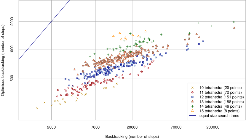
Figure 9: Number of nodes in the search tree visited by the naive algorithm and the optimised backtracking procedure for the $500$ first $1$-vertex triangulations of the Hodgson-Weeks census.

Input: A $v$-vertex $n$-tetrahedra triangulation of a closed $3$-manifold $\mathfrak{T}$

1.: If $\mathfrak{T}$ has more than one vertex, apply the crushing and expanding procedure to $\mathfrak{T}$ as described in [4] and [7] respectively. As a result we obtain a number of triangulations $\mathfrak{T}_{1},\ldots,\mathfrak{T}_{m}$, and a number of “removed components” $c_{1},\ldots,c_{\ell}$ with the following properties.

• Every triangulation $\mathfrak{T}_{i}$, $1\leq i\leq m$, is a $1$-vertex triangulation;

• If $n_{i}$ is the number of tetrahedra in $\mathfrak{T}_{i}$, then $\ell+\sum\limits_{i=0}^{m}n_{i}\leq n;$

• Every “removed component” is either a $3$-sphere, the lens space $L(3,1)$, or the real projective space $\mathbb{R}P^{3}$. Note that homology calculations can distinguish between all of these pieces in polynomial time;

• We have for the topological type of the $\mathfrak{T}_{i}$ that $\mathfrak{T}$ is the connected sum:

  $$\mathfrak{T}\cong\mathfrak{T}_{1}\#\ldots\#\mathfrak{T}_{m}\#c_{1}\#\ldots\#c_{\ell}.$$ (4)

If $\mathfrak{T}$ contains a two-sided projective plane the crushing procedure will detect this fact and the computation is cancelled. The total running time of this step is polynomial.

2.: Compute $\mathrm{TV}_{r,1}(\mathfrak{T}_{i},[0])$, $1\leq i\leq m$.

3.: For all $\mathfrak{T}_{i}$, compute $\mathrm{TV}_{3,1}(\mathfrak{T}_{i})$, and use Theorem 5.3 to obtain $\mathrm{TV}_{r,1}(\mathfrak{T}_{i})$. The Turaev-Viro invariants of $S^{3}$, $\mathbb{R}P^{3}$, and $L(3,1)$ are well known (see Sokolov [19]) and the respective values for the $c_{i}$ can efficiently be pre-computed. If one of the components $c_{i}$ is a real projective space, return $0$, as $\mathrm{TV}_{r,1}(\mathbb{R}P^{3})=0$ for all $r\geq 3$, odd.

4.: Scale all values from the previous step to $\mathrm{TV}_{r,1}^{\prime}$, multiply them and re-scale the product. The result equals $\mathrm{TV}_{r,1}(\mathfrak{T})$, by Theorem 5.2 and Equation (4).

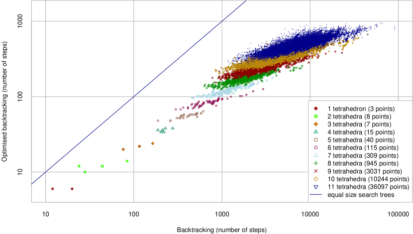
Figure 10: Number of nodes in the search tree visited by the optimised backtracking procedure over the naive algorithm for the $50,814$ $1$-vertex minimal closed triangulations.

Running time, efficiency and effectiveness of the proposed algorithm: The simplifying step, the crushing and expanding procedure, and computing $\mathrm{TV}_{3,1}(\mathfrak{T})$ are all polynomial time algorithms [4, 7]. Following Corollary 2 and Proposition 3 the running time to compute $\mathrm{TV}_{r,1}(\mathfrak{T}_{i},[0])$ is $O(\left\lfloor r/2\right\rfloor^{n_{i}+1})$ (remember, $\mathfrak{T}_{1}$ is a $1$-vertex triangulation). The overall running time is thus $O(\left\lfloor r/2\right\rfloor^{n+1})$. The same procedure can be applied to improve the fixed parameter tractable algorithm as presented in [6]—which is also based on enumerating colourings—to get the running time $O(n\lfloor r/2\rfloor^{6(k+1)}k^{2}\log r)$, where $k$ is the treewidth of the dual graph of $\mathfrak{T}$.

To compare the performance of the naive backtracking with the proposed algorithm, we count the number of nodes in the search tree visited by both algorithms for computing $\mathrm{TV}_{5,1}$ (i) for the first $500$ triangulations of the Hodgson-Weeks census, with $10\leq n\leq 15$, [11], and (ii) for all triangulations with $\leq 11$ tetrahedra in the census of closed minimal triangulations [3], see Figure 9 and 10. These triangulations all have $1$ vertex, and the improvement is solely due to the reduction of the space of colourings studied in this section (in particular, the crushing step is not applied). Improvements in the minimal triangulations census range from factors $2$ to $117$. Improvements in the Hodgson-Weeks census, which contains larger triangulations, range from factors $5.6$ to $215$. Observe how the range of improvements rapidly grows larger as the size of the triangulations increase.

As evidence for the effectiveness of the algorithm, we analyse the ability of $\mathrm{TV}_{r,1}$, $r\in\{3,5,7,9\}$, to distinguish $3$-manifolds from the $3$-sphere $S^{3}$. Since homology can be computed in polynomial time, we only consider $\mathbb{Z}$-homology spheres, i.e., $3$-manifolds with the homology groups of $S^{3}$. There are $36$ distinct $\mathbb{Z}$-homology spheres of complexity at most $11$, meaning, they can be triangulated with $11$ tetrahedra or less. Due to Corollary 1 we already know that none of them can be distinguished from $S^{3}$ by $\mathrm{TV}_{3,1}$ (note that $\mathbb{Z}$-homology spheres are always $\mathbb{Z}_{2}$-homology spheres). $\mathrm{TV}_{5,1}$, $\mathrm{TV}_{7,1}$, and $\mathrm{TV}_{9,1}$, distinguish $22$, $31$, and $30$ of them from $S^{3}$. Furthermore, a combination of $\mathrm{TV}_{5,1}$ and $\mathrm{TV}_{7,1}$ only fails once, and a combination of all three invariants never fails to distinguish $\mathbb{Z}$-homology spheres of complexity $\leq 11$ from $S^{3}$. See Tables 4 and 5 for details.

$n$	$\mathrm{TV}_{3,1}$	$\mathrm{TV}_{4,1}$	$\mathrm{TV}_{5,1}$	$\mathrm{TV}_{6,1}$	$\mathrm{TV}_{7,1}$	$\mathrm{TV}_{8,1}$	$\mathrm{TV}_{9,1}$	$\mathrm{TV}_{5,1}$ and $\mathrm{TV}_{7,1}$
$5$	0/1	0/1	1/1	0/1	1/1	1/1	1/1	1/1
$7$	0/1	0/1	1/1	0/1	1/1	0/1	1/1	1/1
$8$	0/3	0/3	1/3	0/3	3/3	3/3	3/3	3/3
$9$	0/4	0/4	3/4	0/4	3/4	1/4	3/4	4/4
$10$	0/8	0/8	5/8	0/8	7/8	3/8	6/8	8/8
$11$	0/19	0/19	11/19	0/19	16/19	13/19	16/19	18/19

Table 4: Summary of the ability of $\mathrm{TV}_{r,1}$, $3\leq r\leq 9$, to distinguish $\mathbb{Z}$-homology spheres up to complexity $11$ from the $3$-sphere. X/Y denotes the success rate, i.e., there are Y manifolds, X of which can be distinguished from the $3$-sphere by the respective invariant.

$n$	top. type	$\mathrm{TV}_{3,1}$	$\mathrm{TV}_{4,1}$	$\mathrm{TV}_{5,1}$	$\mathrm{TV}_{6,1}$	$\mathrm{TV}_{7,1}$	$\mathrm{TV}_{8,1}$	$\mathrm{TV}_{9,1}$
$5$	$\Sigma(2,3,5)$	$0$	$0$	$1$	$0$	$1$	$1$	$1$
$7$	$\Sigma(2,3,7)$	$0$	$0$	$1$	$0$	$1$	$0$	$1$
$8$	$\Sigma(2,3,11)$	$0$	$0$	$0$	$0$	$1$	$1$	$1$
	$\Sigma(3,4,5)$	$0$	$0$	$0$	$0$	$1$	$1$	$1$
	$\operatorname{SFS}[D:(2,1)(3,1)]\cup_{0,1|1,0}\operatorname{SFS}[D:(2,1)(3,2)]$	$0$	$0$	$1$	$0$	$1$	$1$	$1$
$9$	$\Sigma(2,3,13)$	$0$	$0$	$1$	$0$	$0$	$1$	$1$
	$\Sigma(2,3,17)$	$0$	$0$	$1$	$0$	$1$	$0$	$0$
	$\Sigma(2,5,7)$	$0$	$0$	$1$	$0$	$1$	$0$	$1$
	$\Sigma(3,4,7)$	$0$	$0$	$0$	$0$	$1$	$0$	$1$
$10$	$\Sigma(2,3,19)$	$0$	$0$	$0$	$0$	$1$	$1$	$0$
	$\Sigma(2,3,23)$	$0$	$0$	$1$	$0$	$1$	$0$	$1$
	$\Sigma(2,7,9)$	$0$	$0$	$0$	$0$	$1$	$0$	$1$
	$\Sigma(3,5,11)$	$0$	$0$	$0$	$0$	$1$	$0$	$1$
	$\Sigma(3,7,8)$	$0$	$0$	$1$	$0$	$0$	$0$	$0$
	$\operatorname{SFS}[D:(2,1)(3,1)]\cup_{0,1|1,0}\operatorname{SFS}[D:(2,1)(7,5)]$	$0$	$0$	$1$	$0$	$1$	$0$	$1$
	$\operatorname{SFS}[D:(2,1)(5,2)]\cup_{0,1|1,0}\operatorname{SFS}[D:(2,1)(5,3)]$	$0$	$0$	$1$	$0$	$1$	$1$	$1$
	$\operatorname{Hyp}1.39850888$	$0$	$0$	$1$	$0$	$1$	$1$	$1$
$11$	$\Sigma(2,3,25)$	$0$	$0$	$1$	$0$	$1$	$0$	$1$
	$\Sigma(2,3,29)$	$0$	$0$	$0$	$0$	$0$	$1$	$1$
	$\Sigma(2,5,13)$	$0$	$0$	$1$	$0$	$0$	$1$	$1$
	$\Sigma(2,5,17)$	$0$	$0$	$1$	$0$	$1$	$0$	$0$
	$\Sigma(2,9,11)$	$0$	$0$	$0$	$0$	$1$	$0$	$1$
	$\Sigma(3,4,17)$	$0$	$0$	$0$	$0$	$1$	$0$	$0$
	$\Sigma(3,4,19)$	$0$	$0$	$0$	$0$	$1$	$1$	$0$
	$\Sigma(3,7,13)$	$0$	$0$	$1$	$0$	$0$	$0$	$1$
	$\operatorname{SFS}[D:(2,1)(3,1)]\cup_{-1,2|0,1}\operatorname{SFS}[D:(3,2)(5,3)]$	$0$	$0$	$0$	$0$	$1$	$1$	$1$
	$\operatorname{SFS}[D:(2,1)(3,2)]\cup_{-2,3|-1,2}\operatorname{SFS}[D:(2,1)(5,2)]$	$0$	$0$	$0$	$0$	$1$	$1$	$1$
	$\operatorname{SFS}[D:(2,1)(3,2)]\cup_{0,1|1,0}\operatorname{SFS}[D:(2,1)(11,4)]$	$0$	$0$	$0$	$0$	$1$	$1$	$1$
	$\operatorname{SFS}[D:(2,1)(3,2)]\cup_{0,1|1,0}\operatorname{SFS}[D:(3,2)(5,1)]$	$0$	$0$	$1$	$0$	$1$	$1$	$1$
	$\operatorname{SFS}[D:(2,1)(3,2)]\cup_{0,1|1,0}\operatorname{SFS}[D:(4,1)(5,3)]$	$0$	$0$	$1$	$0$	$1$	$1$	$1$
	$\operatorname{SFS}[D:(2,1)(5,3)]\cup_{0,1|1,0}\operatorname{SFS}[D:(3,2)(4,1)]$	$0$	$0$	$0$	$0$	$1$	$1$	$1$
	$\operatorname{SFS}[D:(2,1)(3,1)]\cup_{-1,1|1,0}\operatorname{SFS}[A:(2,1)]\cup_{0,1|1,1}$	$0$	$0$	$1$	$0$	$1$	$1$	$1$
	$\operatorname{SFS}[D:(2,1)(3,2)]$
	$\operatorname{Hyp}1.73198278$	$0$	$0$	$1$	$0$	$1$	$0$	$1$
	$\operatorname{Hyp}1.91221025$	$0$	$0$	$1$	$0$	$1$	$1$	$1$
	$\operatorname{Hyp}2.22671790$	$0$	$0$	$1$	$0$	$1$	$1$	$1$
	$\operatorname{Hyp}2.25976713$	$0$	$0$	$1$	$0$	$1$	$1$	$1$

Table 5: $\mathbb{Z}$-homology $3$-spheres up to complexity $11$ and the ability of $\mathrm{TV}_{r,1}$, $r\leq 9$ to distinguish them from the $3$-sphere ($0=$ no distinction, $1=$ distinction).

References

- [1] David Bachman. Normalizing topologically minimal surfaces ii: Disks. arXiv:1210.4574, 2012.
- [2] Joan S. Birman. Braids, links, and mapping class groups. Annals of mathematics studies. Princeton University Press, 1975.
- [3] Benjamin A. Burton. Detecting genus in vertex links for the fast enumeration of 3-manifold triangulations. In Proceedings of ISSAC, pages 59–66. ACM, 2011.
- [4] Benjamin A. Burton. A new approach to crushing 3-manifold triangulations. Discrete Comput. Geom., 52(1):116–139, 2014.
- [5] Benjamin A. Burton, Ryan Budney, Will Pettersson, et al. Regina: Software for 3-manifold topology and normal surface theory. http://regina.sourceforge.net/, 1999–2014.
- [6] Benjamin A. Burton, Clément Maria, and Jonathan Spreer. Algorithms and complexity for Turaev-Viro invariants. In Proceedings of ICALP 2015, pages 281–293. Springer, 2015.
- [7] Benjamin A. Burton and Melih Ozlen. A fast branching algorithm for unknot recognition with experimental polynomial-time behaviour. arXiv:1211.1079, 2012.
- [8] Wolfgang Haken. Theorie der Normalflächen. Acta Math., 105:245–375, 1961.
- [9] Joel Hass, Jeffrey C. Lagarias, and Nicholas Pippenger. The computational complexity of knot and link problems. J. Assoc. Comput. Mach., 46(2):185–211, 1999.
- [10] Allen Hatcher. Algebraic Topology. Cambridge University Press, Cambridge, 2002. http://www.math.cornell.edu/~hatcher/AT/ATpage.html.
- [11] Craig D. Hodgson and Jeffrey R. Weeks. Symmetries, isometries and length spectra of closed hyperbolic three-manifolds. Experiment. Math., 3(4):261–274, 1994.
- [12] Robion Kirby and Paul Melvin. The -manifold invariants of Witten and Reshetikhin-Turaev for . Invent. Math., 105(3):473–545, 1991.
- [13] Robion Kirby and Paul Melvin. Local surgery formulas for quantum invariants and the Arf invariant. Geom. Topol. Monogr., pages (7):213–233, 2004.
- [14] Bruce Kleiner and John Lott. Notes on Perelman’s papers. Geom. Topol., 12(5):2587–2855, 2008.
- [15] Sergei Matveev. Algorithmic Topology and Classification of 3-Manifolds. Number 9 in Algorithms and Computation in Mathematics. Springer, Berlin, 2003.
- [16] Sergei Matveev et al. Manifold recognizer. http://www.matlas.math.csu.ru/?page=recognizer, accessed August 2012.
- [17] Justin Roberts. Skein theory and Turaev-Viro invariants. Topology, 34(4):771–787, 1995.
- [18] J. Hyam Rubinstein. Polyhedral minimal surfaces, Heegaard splittings and decision problems for -dimensional manifolds. In Geometric Topology, volume 2 of AMS/IP Stud. Adv. Math., pages 1–20. Amer. Math. Soc., 1997.
- [19] M. V. Sokolov. Which lens spaces are distinguished by Turaev-Viro invariants? Mathematical Notes, 61(3):468–470, 1997.
- [20] John Stillwell. Classical topology and combinatorial group theory, volume 72 of Graduate Texts in Mathematics. Springer-Verlag, New York, second edition, 1993.
- [21] Vladimir G. Turaev. Quantum Invariants of Knots and 3-Manifolds, volume 18 of de Gruyter Studies in Mathematics. Walter de Gruyter & Co., Berlin, revised edition, 2010.
- [22] Vladimir G. Turaev and Oleg Y. Viro. State sum invariants of -manifolds and quantum -symbols. Topology, 31(4):865–902, 1992.