Quantum-Classical Non-Adiabatic Dynamics: Coupled- vs. Independent-Trajectory Methods

Abstract

Trajectory-based mixed quantum-classical approaches to coupled electron-nuclear dynamics suffer from well-studied problems such as the lack of (or incorrect account for) decoherence in the trajectory surface hopping method and the inability of reproducing the spatial splitting of a nuclear wave packet in Ehrenfest-like dynamics. In the context of electronic non-adiabatic processes, these problems can result in wrong predictions for quantum populations and in unphysical outcomes for the nuclear dynamics. In this paper we propose a solution to these issues by approximating the coupled electronic and nuclear equations within the framework of the exact factorization of the electron-nuclear wave function. We present a simple quantum-classical scheme based on coupled classical trajectories, and test it against the full quantum mechanical solution from wave packet dynamics for some model situations which represent particularly challenging problems for the above-mentioned traditional methods.

I Introduction

Non-adiabatic effects often play an important role in the coupled dynamics of electrons and nuclei. Typical examples of processes whose description requires to explicitly account for non-adiabatic electronic transitions induced by the nuclear motion are vision Polli et al. (2010); Hayashi et al. (2009); Chung et al. (2012), photo-synthesis Tapavicza et al. (2011); Brixner et al. (2005), photo-voltaics Rozzi et al. (2013); Silva (2013); Jailaubekov et al. (2013), and charge transport through molecular junctions. Repp et al. (2010); Reckermann et al. (2010); Härtle et al. (2011); Dundas et al. (2009) In all these cases, the electronic effect on the nuclei cannot be expressed by a single adiabatic potential energy surface (PES), corresponding to the occupied eigenstate of the Born-Oppenheimer (BO) Hamiltonian. The exact numerical treatment would in fact require the inclusion of several adiabatic PESs that are coupled via electronic non-adiabatic transitions in regions of strong coupling, such as avoided crossings or conical intersections. Based on this theoretical picture, numerical methods that retain a quantum description of the nuclei have been successfully employed in many applications, e.g. multiple-spawning Martínez and Levine (1996); Martínez et al. (1996); Martínez (2006), multiconfiguration time-dependent Hartree Meyer et al. (1990); Burghardt et al. (1999); Thoss et al. (2004), or non-adiabatic Bohmian dynamics Curchod et al. (2011); Tavernelli (2013); Albareda et al. (2014, 2015); Wyatt et al. (2001); Lopreore and Wyatt (2002); Poirier and Parlant (2007), but actual calculations become unfeasible for systems comprising hundreds or thousands of atoms. Promising alternatives are therefore those approaches that involve a classical or quasi-classical treatment of nuclear motion coupled non-adiabatically to the quantum mechanical motion of the electrons Pechukas (1969a, b); Ehrenfest (1927); Shalashilin (2009); Tully and Preston (1971); Tully (1990); Kohen et al. (1998); Burant and Tully (2000); Prezhdo and Brooksby (2001); Shenvi et al. (2011a); Subotnik et al. (2013); Kapral and Ciccotti (1999); Kapral (2006); Agostini et al. (2007); Shi and Geva (2004); Horenko et al. (2001); Martens and Fang (1997); Bonella and Coker (2001); Huo and Coker (2012); Sun and Miller (1997); Stock and Thoss (1997); Ananth et al. (2007); Miller (2009); Thoss and Wang (2004); Herman (1994); Wu and Herman (2005); Jasper et al. (2004, 2006); Bousquet et al. (2011); Jang (2012); Zimmermann and Vanicek (2012); Hanasaki and Takatsuka (2010); Bonella and Coker (2005); Doltsinis and Marx (2002); Abedi et al. (2014); Prezhdo and Rossky (1997); Zamstein and Tannor (2012). There are two main challenges that theory has to face in this context: (i) The splitting of the nuclear wave packet induced by non-adiabatic couplings needs to be captured in the trajectory-based description. (ii) This requires a clear-cut definition of the classical force in situations when more than a single adiabatic PES is involved.

In the present paper, we attack these two points within the framework of the exact factorization of the electron-nuclear wave function Abedi et al. (2010, 2012). When the solution of the time-dependent Schrödinger equation (TDSE) is written as a single product of a nuclear wave function and an electronic factor, which parametrically depends on the nuclear configuration, two coupled equations of motion for the two components of the full wave function are derived from the TDSE. These equations contain the answer to the above questions. The purpose of this paper is to provide a systematic procedure to develop the necessary approximations when the nuclei are represented in terms of classical trajectories. The final result will be a mixed quantum-classical (MQC) algorithm Min et al. (2015) that we have implemented and tested in various non-adiabatic situations. The numerical scheme presented here is based on the analysis performed so far in the framework of the exact factorization. In previous work, we have first focused on the nuclear dynamics, by analysing the time-dependent potentials Abedi et al. (2013a) of the theory, with particular attention devoted to understanding the fundamental properties that need to be accounted for when introducing approximations. Moreover, we have analyzed the suitability of the classical and quasi-classical treatment Agostini et al. (2013, 2015a, 2015b) of nuclear dynamics, and we have proposed an independent-trajectory MQC scheme Abedi et al. (2014); Agostini et al. (2014) to solve the coupled electronic and nuclear equations within the factorization framework approximately. This result can be viewed as the lowest order version of the algorithm presented here, where refined and more accurate approximations have been introduced.

The new algorithmMin et al. (2015), which is based on a coupled-trajectory (CT) description of nuclear dynamics, will be presented (i) paying particular attention to the physical justification of the approximations introduced, (ii) describing in detail the fundamental equations of the CT-MQC scheme in the form they are implemented in practice, (iii) supporting the analytical derivation with abundant numerical proof of the suitability of the procedure for simulating non-adiabatic dynamics. In particular, we show how the CT procedure compares with the previous MQC Abedi et al. (2014); Agostini et al. (2014) algorithm based on the exact factorization and with the Ehrenfest Ehrenfest (1927) and trajectory surface hopping (TSH) Tully (1990) approaches. This comparison will demonstrate that the CT scheme is able (a) to properly describe the splitting of a nuclear wave packet after the passage through an avoided crossing, related to the steps Abedi et al. (2013a) in the time-dependent potential of the theory, overcoming the limitations of MQC and Ehrenfest, (b) to correctly account for electronic decoherence effects, thus proposing a solution to the over-coherence problem Jasper et al. (2006); Shenvi et al. (2011a); Shenvi and Yang (2012); Subotnik and Shenvi (2011a); Shenvi et al. (2011b); Subotnik (2011); Akimov et al. (2014); Subotnik et al. (2013); Nelson et al. (2013); Prezhdo (1999); Bittner and Rossky (1995, 1997); Cheng et al. (2008); Bedard-Hearn et al. (2005); Granucci and Persico (2007); Granucci et al. (2010); Bajo et al. (2014) affecting TSH.

The paper is organized as follows. The first section focusses on the theory. We construct the algorithm, describe the used approximations and derive the equations that have been implemented. The following section gives a schematic overview of the algorithm, summarizing the results of the first section. The steps to be implemented are described here. The third section shows the numerical results for one-dimensional two-state model systems, representing situations of (a) single avoided crossing, (b) dual avoided crossing, (c) extended coupling with reflection and (d) double arch. Conclusions are drawn in the fourth section.

II Coupled-trajectory mixed quantum-classical algorithm

The exact factorization of the electron-nuclear wave function Abedi et al. (2010, 2012) provides the theoretical background for the development of the algorithm described and tested in this paper. Since the theory has been extensively presented in previous work Abedi et al. (2013a); Agostini et al. (2013); Abedi et al. (2014); Agostini et al. (2014, 2015a, 2015b); Min et al. (2015); Gidopoulos and Gross (2014); Min et al. (2014); Requist et al. ; Suzuki et al. (2014, 2015); Khosravi et al. (2015); Schild et al. (2016), we only refer to Section SI.1 of the Supporting Information for a comprehensive review of the theory.

It has been proved Abedi et al. (2010, 2012) that the solution of the time-dependent Schrödinger equation (TDSE) $[\hat{T}_{n}+\hat{H}_{BO}]\Psi=i\hbar\partial_{t}\Psi$ of a combined system of electrons and nuclei can be written as the product: $\Psi({\underline{\underline{\bf r}}},{\underline{\underline{\bf R}}},t)=\Phi_{\underline{\underline{\bf R}}}({\underline{\underline{\bf r}}},t)\chi({\underline{\underline{\bf R}}},t)$. Here, $\chi({\underline{\underline{\bf R}}},t)$ is the nuclear wave function, which yields the exact nuclear many-body density and current density, whereas $\Phi_{\underline{\underline{\bf R}}}({\underline{\underline{\bf r}}},t)$ is the electronic conditional wave function, which parametrically depends on the nuclear configuration ${\underline{\underline{\bf R}}}$. The squared modulus of $\Phi_{\underline{\underline{\bf R}}}({\underline{\underline{\bf r}}},t)$ is normalized to unity $\forall\,{\underline{\underline{\bf R}}},t$, thus $|\Phi_{\underline{\underline{\bf R}}}({\underline{\underline{\bf r}}},t)|^{2}$ can be interpreted as a conditional probability. The equations of motion describing the time evolution of the two terms of the product are derived by determining the stationary variations Frenkel (1934); Alonso et al. (2013); Abedi et al. (2013b) of the quantum mechanical action with respect to $\Phi_{\underline{\underline{\bf R}}}({\underline{\underline{\bf r}}},t)$ and $\chi({\underline{\underline{\bf R}}},t)$, yielding

$$\Bigg{(}\hat{H}_{BO}+\hat{U}_{en}\left[\Phi_{\underline{\underline{\bf R}}},\chi\right]-\epsilon({\underline{\underline{\bf R}}},t)\Bigg{)}\Phi_{{\underline{\underline{\bf R}}}}({\underline{\underline{\bf r}}},t)=i\hbar\partial_{t}\Phi_{{\underline{\underline{\bf R}}}}({\underline{\underline{\bf r}}},t)$$ (1)

$$\Bigg{(}\sum_{\nu=1}^{N_{n}}\frac{\left[-i\hbar\nabla_{\nu}+{\bf A}_{\nu}({\underline{\underline{\bf R}}},t)\right]^{2}}{2M_{\nu}}+\epsilon({\underline{\underline{\bf R}}},t)\Bigg{)}\chi({\underline{\underline{\bf R}}},t)=i\hbar\partial_{t}\chi({\underline{\underline{\bf R}}},t).$$ (2)

Here the electron-nuclear coupling operator (ENCO) is defined as

$$\hat{U}_{en} \left[\Phi_{\underline{\underline{\bf R}}},\chi\right]=$$

$$\sum_{\nu=1}^{N_{n}}\frac{1}{M_{\nu}}\Bigg{[}\frac{\left[-i\hbar\nabla_{\nu}-{\bf A}_{\nu}({\underline{\underline{\bf R}}},t)\right]^{2}}{2}+\left(\frac{-i\hbar\nabla_{\nu}\chi}{\chi}+{\bf A}_{\nu}({\underline{\underline{\bf R}}},t)\right)\Big{(}-i\hbar\nabla_{\nu}-{\bf A}_{\nu}({\underline{\underline{\bf R}}},t)\Big{)}\Bigg{]}.$$ (3)

The time-dependent vector potential (TDVP) and time-dependent potential energy surface (TDPES) are given by the expressions

$${\bf A}_{\nu}\left({\underline{\underline{\bf R}}},t\right) =\left\langle\Phi_{\underline{\underline{\bf R}}}(t)\right|-i\hbar\nabla_{\nu}\left.\Phi_{\underline{\underline{\bf R}}}(t)\right\rangle_{\underline{\underline{\bf r}}}\,$$ (4)

$$\epsilon({\underline{\underline{\bf R}}},t) =\left\langle\Phi_{\underline{\underline{\bf R}}}(t)\right|\hat{H}_{BO}+\hat{U}_{en}^{coup}-i\hbar\partial_{t}\left|\Phi_{\underline{\underline{\bf R}}}(t)\right\rangle_{\underline{\underline{\bf r}}},$$ (5)

respectively. The numerical procedure referred to as coupled-trajectory mixed quantum-classical (CT-MQC) algorithm, introduced in previous work Min et al. (2015) to solve Eqs. (1) and (2), will be presented here paying special attention to justifying the approximations and describing the implementation of the algorithm.

II.1 The Lagrangian frame

Equations (1) and (2) can be represented on a fixed spatial grid and propagated in time, to compute the evolution of the electronic and nuclear wave functions. However, our aim is to represent the dynamics of quantum nuclei via the motion of a set of coupled classical trajectories, ${\underline{\underline{\bf R}}}^{(I)}(t)$, whose behavior can be assimilated to that of a moving grid. In turn, the dynamics of the electrons is governed by Eq. (1) along each nuclear trajectory. Figure 1 shows the idea behind such representation of the nuclei in terms of classical trajectories: on the left, a molecular wave function (or better the density from a molecular wave function) is plotted on a fixed grid in ${\underline{\underline{\bf r}}},{\underline{\underline{\bf R}}}$ space; on the right, some information along the ${\underline{\underline{\bf R}}}$-direction is lost, since the wave function is available only at the positions of the trajectories, located where the nuclear density is larger. Therefore, it seems more natural to work in a reference frame that moves with the trajectories, the Lagrangian frame, rather than fixed Eulerian frame, and to introduce the approximations starting from this picture. In the Lagrangian frame time-derivatives are calculated “along the flow”, thus all partial time-derivatives have to be replaced by total derivatives, using the chain rule $d/dt=\partial_{t}+\sum_{\nu}\mathbf{V}_{\nu}\cdot\nabla_{\nu}$. Here, the quantity $\mathbf{V}_{\nu}$ is the velocity of the moving grid point, i.e. the velocity of each trajectory which can be determined from the equations below.

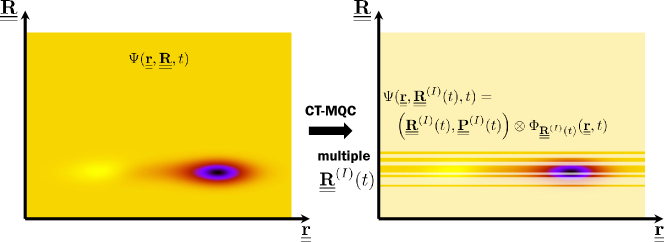
Figure 1: Full molecular wave function (left) as function of electronic (${\underline{\underline{\bf r}}}$) and nuclear (${\underline{\underline{\bf R}}}$) coordinates and its approximation (right) on a set of nuclear trajectories (${\underline{\underline{\bf R}}}^{(I)}(t)$’s). In this case, the molecular wave function is known only at the given positions ${\underline{\underline{\bf R}}}^{(I)}(t)$.

We introduce now the first approximation, namely we derive the classical Newton’s equation from the TDSE (2). We have previously proposed Agostini et al. (2014); Abedi et al. (2014); Min et al. (2015) a derivation based on the complex phase-representation van Vleck (1928) of $\chi({\underline{\underline{\bf R}}},t)$. Here, we present an alternative procedure Agostini et al. (2015a), by writing the nuclear wave function in polar form, $\chi({\underline{\underline{\bf R}}},t)=|\chi({\underline{\underline{\bf R}}},t)|e^{(i/\hbar)S({\underline{\underline{\bf R}}},t)}$. Then, the real part of Eq. (2) yields

$$\frac{\partial}{\partial t}S({\underline{\underline{\bf R}}},t)=-\sum_{\nu=1}^{N_{n}}\frac{\left[\nabla_{\nu}S({\underline{\underline{\bf R}}},t)+{\bf A}_{\nu}({\underline{\underline{\bf R}}},t)\right]^{2}}{2M_{\nu}}-\epsilon({\underline{\underline{\bf R}}},t)+\hbar^{2}\sum_{\nu=1}^{N_{n}}\frac{1}{2M_{\nu}}\frac{\nabla_{\nu}^{2}|\chi({\underline{\underline{\bf R}}},t)|}{|\chi({\underline{\underline{\bf R}}},t)|},$$ (6)

a Hamilton-Jacobi equation (HJE) in the presence of the TDVP ${\bf A}_{\nu}({\underline{\underline{\bf R}}},t)$ and of a potential term (last term in Eq. (6)) known in the framework of Bohmian dynamics as quantum potential. The imaginary part of Eq. (2) yields a continuity equation for the nuclear density. Neglecting the quantum potential, Eq. (6) becomes a (standard) classical HJE,

$$\dot{S}({\underline{\underline{\bf R}}},t)=-\sum_{\nu=1}^{N_{n}}\Bigg{[}\frac{\left[\nabla_{\nu}S({\underline{\underline{\bf R}}},t)+{\bf A}_{\nu}({\underline{\underline{\bf R}}},t)\right]^{2}}{2M_{\nu}}-\mathbf{V}_{\nu}\cdot\nabla_{\nu}S({\underline{\underline{\bf R}}},t)\Bigg{]}-\epsilon({\underline{\underline{\bf R}}},t),$$ (7)

where $\dot{S}$ stands for the full time derivative of $S$. In previous work Agostini et al. (2014); Abedi et al. (2014), rather than $S({\underline{\underline{\bf R}}},t)$, the HJE contained $S_{0}({\underline{\underline{\bf R}}},t)$, the lowest order term in an expansion of the complex phase in powers of Planck’s constant. The comparison with this result Agostini et al. (2015b) allows us to define the canonical momentum of the moving grid $M_{\nu}\mathbf{V}_{\nu}=\nabla_{\nu}S_{0}({\underline{\underline{\bf R}}},t)+{\bf A}_{\nu}({\underline{\underline{\bf R}}},t)=\mathbf{P}_{\nu}$. Taking the spatial derivative $\nabla_{\nu^{\prime}}$ on both sides, Eq. (7) reduces to a classical evolution equation for the characteristics

$$\dot{\mathbf{P}}_{\nu}(t)\Big{|}_{{\underline{\underline{\bf R}}}^{(I)}(t)}= -\nabla_{\nu}\left(\epsilon({\underline{\underline{\bf R}}},t)+\sum_{\nu^{\prime}=1}^{N_{n}}{\bf A}_{\nu^{\prime}}({\underline{\underline{\bf R}}},t)\cdot\frac{\bf P_{\nu^{\prime}}({\underline{\underline{\bf R}}},t)}{M_{\nu}}\right)+\dot{\bf A}_{\nu}({\underline{\underline{\bf R}}},t)\Bigg{|}_{{\underline{\underline{\bf R}}}^{(I)}(t)}.$$ (8)

At time $t$ all quantities are evaluated at the grid point ${\underline{\underline{\bf R}}}^{(I)}(t)$.

Eq. (8) identifies the classical force used to evolve the grid points ${\underline{\underline{\bf R}}}^{(I)}(t)$. In the proposed implementation, (i) at the initial time $N_{traj}$ points will be sampled from the probability distribution associated to the initial nuclear density $|\chi({\underline{\underline{\bf R}}},t=0)|^{2}$, (ii) the time-evolved of those points will give information about the molecular wave function in the regions of nuclear configuration space of large probability at every time, as shown in Fig. 1 (iii) the nuclear density at time $t$ can be reconstructed from a histogram Abedi et al. (2014); Agostini et al. (2014, 2015a) representing the distribution of classical trajectories.

II.2 Choice of the gauge

It is straightforward to prove, as described in Section SI.1 of the Supporting Information, that the product form the electron-nuclear wave function is invariant under a $({\underline{\underline{\bf R}}},t)$-phase transformation of $\Phi_{\underline{\underline{\bf R}}}({\underline{\underline{\bf r}}},t)$ and $\chi({\underline{\underline{\bf R}}},t)$. In order to fix this gauge freedom, Eqs. (1) and (2) have to be solved with an additional constraint, which is chosen in this case to be

$$\epsilon({\underline{\underline{\bf R}}},t)+\sum_{\nu=1}^{N_{n}}{\bf A}_{\nu}({\underline{\underline{\bf R}}},t)\cdot\frac{{\bf P}_{\nu}({\underline{\underline{\bf R}}},t)}{M_{\nu}}=0.$$ (9)

This condition is imposed in both the electronic and nuclear equations. In particular, Eq. (8) simplifies to $\dot{\mathbf{P}}_{\nu}(t)=\dot{\mathbf{A}}_{\nu}(t)$. When the electronic (1) and nuclear (2) equations are integrated by imposing Eq. (9), this gauge condition is automatically satisfied but it should be checked during the evolution in order to test the numerical accuracy.

II.3 Time-dependent potential energy surface

The expression of the TDPES in the Lagrangian frame becomes

$$\epsilon^{apx}({\underline{\underline{\bf R}}},t)=\left\langle\Phi_{\underline{\underline{\bf R}}}(t)\right|\hat{H}_{BO}\left|\Phi_{\underline{\underline{\bf R}}}(t)\right\rangle_{\underline{\underline{\bf r}}}-i\hbar\left\langle\Phi_{\underline{\underline{\bf R}}}(t)\right|\left.\dot{\Phi}_{\underline{\underline{\bf R}}}(t)\right\rangle_{\underline{\underline{\bf r}}}-\sum_{\nu=1}^{N_{n}}\frac{\bf P_{\nu}}{M_{\nu}}\cdot\mathbf{A}_{\nu}({\underline{\underline{\bf R}}},t),$$ (10)

where we have introduced here the second approximation, namely we have neglected the first term on the right-hand-side in the definition (II) of the ENCO. This term contains second-order derivatives of the electronic wave function with-respect-to the nuclear positions, whose calculation requires a larger numerical effort than first-order derivatives. Studies have shown that this term is indeed negligible Scherrer et al. (2015) if compared to the leading contribution, i.e. the second term on the right-hand-side of Eq. (II). Furthermore, the term containing the second-order derivatives is the only term that contributes to the TDPES, the other being identically zero when averaged over $\Phi_{\underline{\underline{\bf R}}}({\underline{\underline{\bf r}}},t)$. Therefore, in order to maintain gauge-invariance, the ENCO cannot appear Abedi et al. (2013a); Agostini et al. (2013) in the expression of the TDPES, as it is clear in Eq. (10). Moreover, Eq. (10) is obtained by replacing the partial time-derivative from Eq. (5) with the total time-derivative. The additional term from the chain rule used above contains $\nabla_{\nu}$, which leads to the appearance of the TDVP when averaged over the electronic wave function.

II.4 The Born-Huang expansion

Classical trajectories evolve according to the force in Eq. (8), where the gauge condition (9) is imposed at each time, and are coupled to an approximated form of the electronic equation, namely

$$i\hbar\dot{\Phi}_{\underline{\underline{\bf R}}}({\underline{\underline{\bf r}}},t)= \Bigg{[}\hat{H}_{BO}+\sum_{\nu=1}^{N_{n}}\frac{1}{M_{\nu}}\left(\frac{-i\hbar\nabla_{\nu}\chi({\underline{\underline{\bf R}}},t)}{\chi({\underline{\underline{\bf R}}},t)}+{\bf A}_{\nu}({\underline{\underline{\bf R}}},t)-{\mathbf{P}}_{\nu}(t)\right)\left(-i\hbar\nabla_{\nu}\right)\Bigg{]}\Phi_{\underline{\underline{\bf R}}}({\underline{\underline{\bf r}}},t)$$

$$-\Bigg{[}\sum_{\nu=1}^{N_{n}}\frac{1}{M_{\nu}}\left(\frac{-i\hbar\nabla_{\nu}\chi({\underline{\underline{\bf R}}},t)}{\chi({\underline{\underline{\bf R}}},t)}+{\bf A}_{\nu}({\underline{\underline{\bf R}}},t)\right){\bf A}_{\nu}({\underline{\underline{\bf R}}},t)+\epsilon^{apx}({\underline{\underline{\bf R}}},t)\Bigg{]}\Phi_{\underline{\underline{\bf R}}}({\underline{\underline{\bf r}}},t),$$ (11)

where we have replaced once again the partial time-derivative with the total derivative, according to $\partial_{t}\Phi_{{\underline{\underline{\bf R}}}}({\underline{\underline{\bf r}}},t)\big{|}_{{\underline{\underline{\bf R}}}^{(I)}(t)}=\dot{\Phi}_{{\underline{\underline{\bf R}}}}({\underline{\underline{\bf r}}},t)-\sum_{\nu=1}^{N_{n}}\frac{\mathbf{P}_{\nu}(t)}{M_{\nu}}\cdot\nabla_{\nu}\Phi_{{\underline{\underline{\bf R}}}}({\underline{\underline{\bf r}}},t)\big{|}_{{\underline{\underline{\bf R}}}^{(I)}(t)}$. Notice that all quantities in Eq. (11) are evaluated along the classical trajectories ${\underline{\underline{\bf R}}}^{(I)}(t)$ and that no further approximation than those described so far has been used to derive this expression. In the numerical scheme proposed here Min et al. (2015), the electronic wave function is expanded according to the so-called Born-Huang expansion in terms of the adiabatic states $\varphi_{\underline{\underline{\bf R}}}^{(l)}({\underline{\underline{\bf r}}})$, which are eigenstates of the Hamiltonian $\hat{H}_{BO}$ with eigenvalues $\epsilon_{BO}^{(l)}({\underline{\underline{\bf R}}})$. Inserting the expansion

$$\Phi_{{\underline{\underline{\bf R}}}}({\underline{\underline{\bf r}}},t)=\sum_{l}C_{l}\left({\underline{\underline{\bf R}}},t\right)\varphi_{\underline{\underline{\bf R}}}^{(l)}({\underline{\underline{\bf r}}})$$ (12)

in Eq. (11), we derive a set of coupled partial differential equations for the coefficients $C_{l}\left({\underline{\underline{\bf R}}},t\right)$

$$\dot{C}_{l}^{(I)}(t)=\frac{-i}{\hbar}\Bigg{[}\epsilon_{BO}^{(l)(I)}-{\epsilon^{apx}}^{(I)}(t)-\sum_{\nu=1}^{N_{n}}\frac{\mathbf{P}_{\nu}^{(I)}(t)+i\boldsymbol{\mathcal{P}}_{\nu}^{(I)}(t)}{M_{\nu}}\cdot\mathbf{A}_{\nu}(t)\Bigg{]}C_{l}^{(I)}(t)- \sum_{\nu=1}^{N_{n}}\frac{i\boldsymbol{\mathcal{P}}_{\nu}^{(I)}(t)}{M_{\nu}}\nabla_{\nu}C_{l}^{(I)}(t)$$

$$-\sum_{\nu=1}^{N_{n}}\frac{\mathbf{P}_{\nu}^{(I)}(t)+i\boldsymbol{\mathcal{P}}_{\nu}^{(I)}(t)}{M_{\nu}}\sum_{k} C_{k}^{(I)}(t)\mathbf{d}_{\nu,lk}^{(I)}.$$ (13)

The non-adiabatic coupling vectors (NACVs) have been introduced in the above expression, i.e. $\mathbf{d}_{\nu,lk}^{(I)}=\langle\varphi_{{\underline{\underline{\bf R}}}^{(I)}(t)}^{(l)}|\nabla_{\nu}\varphi_{{\underline{\underline{\bf R}}}^{(I)}(t)}^{(k)}\rangle_{\underline{\underline{\bf r}}}$. We have used here a superscript $(I)$ to indicate that all quantities depending on ${\underline{\underline{\bf R}}}$ are to be calculated at the position ${\underline{\underline{\bf R}}}^{(I)}(t)$ at time $t$. Henceforth, the spatial dependence will only be indicated by such superscript symbol. In deriving Eq. (II.4), we have employed the polar representation of the nuclear wave function in $\hat{U}_{en}$ of Eq. (II), i.e.

$$\frac{-i\hbar\nabla_{\nu}\chi^{(I)}(t)}{\chi^{(I)}(t)}+\mathbf{A}_{\nu}^{(I)}(t) =\left[\nabla_{\nu}S^{(I)}(t)+\mathbf{A}_{\nu}^{(I)}(t)\right]+i\frac{-\hbar\nabla_{\nu}\left|\chi^{(I)}(t)\right|}{\left|\chi^{(I)}(t)\right|}$$

$$=\mathbf{P}_{\nu}^{(I)}(t)+i\boldsymbol{\mathcal{P}}_{\nu}^{(I)}(t).$$ (14)

This equation contains the quantities $\mathbf{P}_{\nu}^{(I)}(t)$ and $\boldsymbol{\mathcal{P}}_{\nu}^{(I)}(t)$, which will be discussed in detail below.

Let us now introduce the gauge condition (9) in Eq. (II.4), namely

$$\dot{C}_{l}^{(I)}(t)=\frac{-i}{\hbar}\Bigg{[}\epsilon_{BO}^{(l)(I)}-\sum_{\nu=1}^{N_{n}}\frac{i\boldsymbol{\mathcal{P}}_{\nu}^{(I)}(t)}{M_{\nu}}\cdot\mathbf{A}_{\nu}(t)\Bigg{]}C_{l}^{(I)}(t)-\sum_{\nu=1}^{N_{n}}\frac{i\boldsymbol{\mathcal{P}}_{\nu}^{(I)}(t)}{M_{\nu}}\nabla_{\nu}C_{l}^{(I)}(t)$$

$$-\sum_{\nu=1}^{N_{n}}\frac{\mathbf{P}_{\nu}(t)+i\boldsymbol{\mathcal{P}}_{\nu}^{(I)}(t)}{M_{\nu}}\sum_{k}C_{k}^{(I)}(t)\mathbf{d}_{\nu,lk}^{(I)}.$$ (15)

This preserves the norm of the electronic wave function along the time evolution. On the right-hand-side of Eq. (II.4), the terms not containing $\boldsymbol{\mathcal{P}}_{\nu}^{(I)}(t)$ are exactly the same as in other algorithms, i.e. Ehrenfest and TSH. The additional terms follow from the exact factorization and are all proportional to $\boldsymbol{\mathcal{P}}_{\nu}^{(I)}(t)$, the so-called quantum momentum, that will be discussed below. Moreover, since the coefficients in the expansion (12) depend on nuclear positions, spatial derivatives of such coefficients need to be taken into account.

II.5 Spatial dependence of the coefficients of the Born-Huang expansion

The coefficients $C_{l}^{(I)}(t)$ of the Born-Huang expansion of the electronic wave function are written in terms of the their modulus $\left|C_{l}^{(I)}(t)\right|$ and phase $\gamma_{l}^{(I)}(t)$,

$$\nabla_{\nu}C_{l}^{(I)}(t) =\left[\frac{\nabla_{\nu}\left|C_{l}^{(I)}(t)\right|}{\left|C_{l}^{(I)}(t)\right|}+\frac{i}{\hbar}\nabla_{\nu}\gamma_{l}^{(I)}(t)\right]C_{l}^{(I)}(t).$$ (16)

The third approximation introduced to derive the CT-MQC algorithm consists in (i) neglecting the first term on the right-hand-side of the above equation and (ii) neglecting all terms depending on the NACVs in the expression of the remaining term. Based on the analysis reported in previous work Abedi et al. (2013a); Agostini et al. (2013, 2015a), the contribution of the first term is indeed negligible if compared to the spatial derivative of the phase $\gamma_{l}^{(I)}(t)$. We will present our argument below and we will give the expression of the remaining term. A semiclassical analysis is provided in Section SI.2 of the Supporting Information.

Based on the solution of the full TDSE Abedi et al. (2013a); Agostini et al. (2013, 2015a) for one-dimensional systems, we have observed that at a given time the quantities $\left|C_{l}({\underline{\underline{\bf R}}},t)\right|$ are either constant functions of ${\underline{\underline{\bf R}}}$ or present a sigmoid shape Agostini et al. (2015a). In particular, this second feature appears when the nuclear wave packet splits after having crossed a region of strong coupling. In regions where the $\left|C_{l}({\underline{\underline{\bf R}}},t)\right|$’s are constant, their derivatives are zero, thus our approximation holds perfectly; in the sigmoid case, $\left|C_{l}({\underline{\underline{\bf R}}},t)\right|$ is constant, i.e. either 0 or 1, far from the step of the sigmoid function, and linear around the center of the step. Furthermore, the center of the step is the position where the nuclear density splits Abedi et al. (2013a), and only in this region the gradient of $\left|C_{l}({\underline{\underline{\bf R}}},t)\right|$ can be significantly different from zero. We have analytically demonstrated that these properties are generally valid Agostini et al. (2015a) in the absence of external time-dependent fields. It is important to keep in mind that the nuclear density is reconstructed from the distribution of classical trajectories, thus it seems reasonable to assume that when the nuclear density splits into two or more branches, the probability of finding trajectories in the tail regions is very small. It follows that $\nabla_{\nu}|C_{l}^{(I)}|/|C_{l}^{(I)}|=0$ is an approximation only for few trajectories, located in the tail regions, while it is true for all other trajectories. Therefore, we expect that such an approximation will not affect drastically the final (averaged over all trajectories) results.

We now come back to the expression of $\nabla_{\nu}\gamma_{l}^{(I)}(t)$. First of all, let us show the time derivative of $\gamma_{l}^{(I)}(t)$, namely $\dot{\gamma}_{l}^{(I)}(t)=-\epsilon_{BO}^{(l),(I)}+\mbox{non-adiabatic terms}$. The derivation of the additional “non-adiabatic terms”, containing the NACVs is tedious and only requires the knowledge of Eq. (II.4). If we assume that the NACVs are localized in space, that is an approximation which is valid in many physically relevant situations Tapavicza et al. (2007); Worth et al. (2003); Burghardt et al. (2004); Doltsinis and Marx (2002), we can simply write $\nabla_{\nu}\dot{\gamma}_{l}^{(I)}(t)=-\nabla_{\nu}\epsilon_{BO}^{(l)}$ or, equivalently,

$$\nabla_{\nu}\gamma_{l}^{(I)}(t)=-\int^{t}dt^{\prime}\nabla_{\nu}\epsilon_{BO}^{(l),(I)}=\mathbf{f}_{l,\nu}^{(I)}(t).$$ (17)

Therefore, the approximate form of the spatial derivative of the coefficient of the Born-Huang expansion becomes $\nabla_{\nu}C_{l}^{(I)}(t)=(i/\hbar)\mathbf{f}_{l,\nu}^{(I)}(t)C_{l}^{(I)}(t)$. The quantity $\mathbf{f}_{l,\nu}^{(I)}(t)$, the time-integrated adiabatic force, can be determined by only computing electronic adiabatic properties. It follows that the electronic evolution equation (II.4) is no longer a partial differential equation, but rather an ordinary differential equation.

Related to the discussion just presented, we can now give the explicit expression of the TDVP in terms of the adiabatic electronic properties, namely

$${\bf A}_{\nu}^{(I)}(t)=\sum_{l=1}^{N_{st}}\rho_{ll}^{(I)}(t)\mathbf{f}_{l,\nu}^{(I)}(t)+\hbar\operatorname{Im}\sum_{l,k=1}^{N_{st}}\rho_{lk}^{(I)}(t)\mathbf{d}_{\nu,lk}^{(I)},$$ (18)

with $\rho_{lk}^{(I)}(t)=C_{l}^{(I)*}(t)C_{k}^{(I)}(t)$ the elements of the electronic density matrix.

II.6 Quantum momentum

The crucial difference between standard Ehrenfest-type approaches and our new quantum-classical algorithm for non-adiabatic dynamics is the appearance of the quantum momentum in the equations of motion. In the framework of the exact factorization, the electronic equation (1) contains the exact coupling to the nuclei, which is expressed in terms of $-i\hbar\nabla_{\nu}\chi/\chi$. As in Eq. (14), this dependence on the nuclear wave function is written as

$$\frac{-i\hbar\nabla_{\nu}\chi^{(I)}(t)}{\chi^{(I)}(t)}+\mathbf{A}_{\nu}^{(I)}(t)=\mathbf{P}_{\nu}^{(I)}(t)+i\boldsymbol{\mathcal{P}}_{\nu}^{(I)}(t).$$ (19)

In writing the first term on the right-hand-side, we are using the first approximation introduced above, where the gradient of the phase of the nuclear wave function (see Eq. (14) for comparison) is truncated at the zero-th order term in the $\hbar$-expansion. The second term is the quantum momentum, related to the spatial variation of the nuclear density (notice that the relation $\nabla_{\nu}|\chi|/|\chi|=\nabla_{\nu}|\chi|^{2}/(2|\chi|^{2})$ holds). This term, which has the dimension of a momentum and is purely imaginary, is a known quantity in the context of Bohmian mechanics Garashchuk and Rassolov (2003). When presenting the numerical results, it will become clear that the quantum momentum is the source of decoherence effects on electronic dynamics.

In the nuclear equation (7) we have discarded the quantum potential, while in the electronic equation (II.4) we have taken the quantum momentum into account. On the one hand, the quantum potential appears $\mathcal{O}(\hbar^{2})$, while the correction to the nuclear momentum is $\mathcal{O}(\hbar)$, thus our approximations are consistent up to within this order in Planck’s constant. On the other hand, we have already shown Agostini et al. (2014) that neglecting the quantum momentum in the electronic equation from the exact factorization produces an Ehrenfest-like evolution, where the spatial splitting of the nuclear wave packet cannot be captured. The introduction of the quantum momentum is thus essential. Further studies on incorporating the quantum potential in Eq. (7) following the strategies such as the ones discussed in the context of Bohmian dynamics Curchod and Tavernelli (2013); Curchod et al. (2011) are indeed a route to be investigated.

The calculation of the quantum momentum requires calculation of the spatial derivatives of the nuclear density, which is known numerically only at the positions of the classical trajectories. Therefore, in order to evaluate such derivative at the position ${\underline{\underline{\bf R}}}^{(I)}(t)$, non-local information about the position of neighboring trajectories ${\underline{\underline{\bf R}}}^{(J)}(t)$ is necessary. This requirement is what makes the algorithm based on Eqs. (8) and (II.4) a coupled-trajectory scheme. The procedure to calculate the quantum momentum used in the current implementation of the algorithm is described below for a two-level system, since all numerical tests are performed on such model situations. The extension to a multi-level system is presented in Section SI.3 of the Supporting Information.

II.6.1 Two-level system

The nuclear density can be expressed as the sum of BO-projected densities. In Section SI.1 of the Supporting Information it is proved that if the full wave function $\Psi$ is expanded on the adiabatic basis with coefficients $F_{l}({\underline{\underline{\bf R}}},t)$, then the factorization $\Psi=\Phi_{\underline{\underline{\bf R}}}\chi$ implies that $|\chi|^{2}=\sum_{l}|F_{l}|^{2}$ and $F_{l}=C_{l}\chi$. Therefore, in a two-level system the quantum momentum becomes

$$\boldsymbol{\mathcal{P}}({\underline{\underline{\bf R}}},t)=\frac{-\hbar}{2}\frac{\nabla_{\nu}\left|\chi({\underline{\underline{\bf R}}},t)\right|^{2}}{\left|\chi({\underline{\underline{\bf R}}},t)\right|^{2}}=\frac{-\hbar}{2}\frac{\nabla_{\nu}\left|F_{1}({\underline{\underline{\bf R}}},t)\right|^{2}+\nabla_{\nu}\left|F_{2}({\underline{\underline{\bf R}}},t)\right|^{2}}{\left|F_{1}({\underline{\underline{\bf R}}},t)\right|^{2}+\left|F_{2}({\underline{\underline{\bf R}}},t)\right|^{2}}.$$ (20)

We now assume that each BO-projected nuclear wave packet is a single Gaussian. Notice that we make this approximation only to evaluate the quantum momentum, whereas the nuclear dynamics will still be represented in terms of classical trajectories. This is the fourth approximation introduced to derive the CT-MQC algorithm. We write

$$\left|F_{l}\left({\underline{\underline{\bf R}}},t\right)\right|^{2}=\rho_{ll}(t)\frac{1}{\mathcal{N}_{l}}\prod_{\nu=1}^{N_{n}}\exp{\left[-\frac{\left[\mathbf{R}_{\nu}-\mathbf{R}_{\nu}^{(l)}(t)\right]^{2}}{\sigma_{l}^{2}(t)}\right]}=\rho_{ll}(t)G_{\sigma_{l}}\left({\underline{\underline{\bf R}}}-{\underline{\underline{\bf R}}}^{(l)}(t)\right)$$ (21)

where $\sigma_{l}(t)$ and $\mathbf{R}_{\nu}^{(l)}(t)$ are the time-dependent variance and mean value, respectively, of the normalized Gaussian $G_{\sigma_{l}}$. $\rho_{ll}(t)$ accounts for the normalization (the integral over ${\underline{\underline{\bf R}}}$ of the function $|F_{l}\left({\underline{\underline{\bf R}}},t\right)|^{2}$ is the population of the corresponding BO state; see for this Section SI.3 of the Supporting Information) and $\mathcal{N}_{l}$ is the normalization constant. Computing the gradient of the Gaussians, the quantum momentum becomes

$$\boldsymbol{\mathcal{P}}({\underline{\underline{\bf R}}},t)=\hbar\sum_{l=1,2}\frac{\left[\mathbf{R}_{\nu}-\mathbf{R}_{\nu}^{(l)}(t)\right]}{\sigma_{l}^{2}(t)}\left|C_{l}({\underline{\underline{\bf R}}},t)\right|^{2}$$ (22)

and this expression can be calculated analytically if the mean position and variance are determined from the distribution of the classical trajectories, according to Agostini et al. (2015a)

$$\mathbf{R}_{\nu}^{(l)}(t) =\frac{1}{\rho_{ll}(t)}\int d{\underline{\underline{\bf R}}}\,\mathbf{R}_{\nu}\left|F_{l}\left({\underline{\underline{\bf R}}},t\right)\right|^{2}\simeq\sum_{I=1}^{N_{traj}}\mathbf{R}_{\nu}^{(I)}(t)\frac{\rho_{ll}^{(I)}(t)}{\sum_{J=1}^{N_{traj}}\rho_{ll}^{(J)}(t)}$$ (23)

$$\sigma_{l}^{2}(t) =\frac{2}{\rho_{ll}(t)}\int d{\underline{\underline{\bf R}}}\,\big{[}\mathbf{R}_{\nu}-\mathbf{R}_{\nu}^{(l)}(t)\big{]}^{2}\left|F_{l}\left({\underline{\underline{\bf R}}},t\right)\right|^{2}\simeq\sum_{I=1}^{N_{traj}}\left[\mathbf{R}_{\nu}^{(I)}(t)-\mathbf{R}_{\nu}^{(l)}(t)\right]^{2}\frac{\rho_{ll}^{(I)}(t)}{\sum_{J=1}^{N_{traj}}\rho_{ll}^{(J)}(t)}.$$ (24)

Here, we have used the following approximations

$$\left|F_{l}\left({\underline{\underline{\bf R}}},t\right)\right|^{2} \simeq\frac{1}{N_{traj}}\sum_{I=1}^{N_{traj}}\rho_{ll}^{(I)}(t)\delta\left({\underline{\underline{\bf R}}}-{\underline{\underline{\bf R}}}^{(I)}(t)\right)$$ (25)

$$\rho_{ll}(t) \simeq\frac{1}{N_{traj}}\sum_{I=1}^{N_{traj}}\rho_{ll}^{(I)}(t),$$ (26)

with $N_{traj}$ the total number of trajectories. The first equation associates a weight, $\rho_{ll}^{(I)}(t)$, to each trajectory, in order to reconstruct the BO-projected densities from the histogram, i.e. $N_{traj}^{-1}\sum_{I}\delta({\underline{\underline{\bf R}}}-{\underline{\underline{\bf R}}}^{(I)}(t))$, which approximates the full nuclear density. The second equation is instead used to determine the population of the adiabatic state $l$ as an average of the coefficients associated with each trajectory. The pre-factor $N_{traj}^{-1}$ stands for the weight of each trajectory, chosen to be constant. In Eqs. (25) and (26), the integrals over the positions ${\underline{\underline{\bf R}}}$ have been replaced by the sum over trajectories since the nuclear density, for each trajectory, is a $\delta$-function centered at the position of the trajectory itself.

An additional simplification can be introduced at this point, based on the following observations. If the quantum momentum $\boldsymbol{\mathcal{P}}_{\nu}({\underline{\underline{\bf R}}},t)$ is neglected in the electronic equation (II.4), then the quantum-classical equations derived from the exact factorization yield Ehrenfest dynamics: the nuclear wave packet propagates coherently and its spatial splitting cannot be reproduced Agostini et al. (2014). In this case the spatial distribution Agostini et al. (2015a) of the coefficients $|C_{l}^{(I)}(t)|$ is not correctly reproduced, as they are more or less constant. The lack of spatial distribution is related to the lack of decoherence: the indicator used in the following analysis to quantify decoherence (see Eq. (30)) depends in fact on the shape of $|C_{l}^{(I)}(t)|$. Also, we have seen in previous studies Agostini et al. (2015a) that steps developing in the exact TDPES, bridging regions of space where it has adiabatic shapes, is instead able to induce the splitting of the nuclear density. Outside the step region, the force is then simply adiabatic (i.e. the gradient of an adiabatic surface). The region of the step is where the additional force, beyond the adiabatic force, acts. Furthermore, the steps in the TDPES appear in the region where $\left|C_{l}({\underline{\underline{\bf R}}},t)\right|$, the moduli of the coefficients in the Born-Huang expansion (12), are neither 0 nor 1 (remember that $\left|C_{l}({\underline{\underline{\bf R}}},t)\right|$ is either constant in space or has a sigmoid shape between the values 0 and 1 Abedi et al. (2013a); Agostini et al. (2013, 2015a)). Therefore, it seems natural to assume that an additional effect, responsible for the splitting of the nuclear density, should be localized in space in the region of the steps in the TDPES, meaning in the region between the two Gaussian-shaped BO densities. There, $\boldsymbol{\mathcal{P}}_{\nu}({\underline{\underline{\bf R}}},t)$ can be represented, approximately, as a linear function, which can be determined analytically. Notice that an analogous treatment of the quantum momentum, which follows from the hypothesis that the nuclear density can be approximated as a sum of Gaussians, has already been discussed in the context of Bohmian mechanics Garashchuk and Rassolov (2003). Due to this approximation, however, the coupled electronic and nuclear equations do not fulfil some fundamental properties, i.e. population exchange between electronic states might be observed even when the NACVs are zero.

The linear function used to approximate the quantum momentum is determined by associating two parameters to it: a $y$-intercept, ${\underline{\underline{\bf R}}}^{0}$, by imposing in Eq. (II.4) that no population variation shall be observed if the NACVs are zero, and a slope, $\alpha$, determined analytically from Eq. (22) evaluated at ${\underline{\underline{\bf R}}}^{0}$. The first parameter is determined by setting the terms containing the NACVs in Eq. (II.4) to zero and then imposing that the remaining part, $\dot{\rho}_{ll}^{(I)}=\sum_{\nu}[2\boldsymbol{\mathcal{P}}_{\nu}^{(I)}/(\hbar M_{\nu})]\cdot[\mathbf{A}_{\nu}^{(I)}-\mathbf{f}_{l,\nu}^{(I)}]\rho^{(I)}_{ll}$ , has to be zero when summed up over the trajectories. When imposing this condition, the expression used for the quantum momentum is simply $\boldsymbol{\mathcal{P}}_{\nu}^{(I)}=\alpha(\mathbf{R}_{\nu}^{(I)}-\mathbf{R}^{0}_{\nu})$. As indicated above, once the $y$-intercept is known, it is inserted into Eq. (22) and the slope is obtained analytically, yielding the quantum momentum as

$$\boldsymbol{\mathcal{P}}_{\nu}^{(I)}(t)=\hbar\left(\sum_{l=1,2}\frac{\left|C_{l}\left({\underline{\underline{\bf R}}},t\right)\right|^{2}\bigg{|}_{\mathbf{R}_{\nu}^{0}(t)}}{\sigma^{2}_{l}(t)}\right)\left[\mathbf{R}_{\nu}^{(I)}(t)-\sum_{J}\mathbf{R}_{\nu}^{(J)}(t)\frac{\rho^{(J)}_{11}(t)\rho^{(J)}_{22}(t)\left(\mathbf{f}_{1,\nu}^{(J)}(t)-\mathbf{f}_{1,\nu}^{(J)}(t)\right)}{\sum_{J}\rho^{(J)}_{11}(t)\rho^{(J)}_{22}(t)\left(\mathbf{f}_{1,\nu}^{(J)}(t)-\mathbf{f}_{1,\nu}^{(J)}(t)\right)}\right]$$ (27)

This expression is only used in the region between the centers of the BO-projected densities, $\mathbf{R}_{\nu}^{(l)}(t)$. Outside this region, the quantum momentum is set zero.

III Numerical Implementation

In this section, we present the numerical implementation of the CT-MQC algorithm. First, we summarize the final expressions of the classical force, used to generate the trajectories, and the evolution equation for the coefficients of the Born-Huang expansion of the electronic wave function. The CT-MQC equations are cast below in such a way that the first line in both expressions is exactly the same as in Ehrenfest-like approaches, while the corrections, in the second line of each expression, are (i) proportional to the quantum momentum, (ii) do not contain the NACVs, i.e. the “competing” effects of population exchange induced by the NACVs and of decoherence induced by the quantum momentum have been separated (this is the fifth approximation introduced in the equations (1) and (2) to derive the CT-MQC algorithm). The classical force

$$\dot{\mathbf{P}}_{\nu}^{(I)}(t) =-\sum_{k}\rho_{kk}^{(I)}(t)\nabla_{\nu}\epsilon_{BO}^{(k),(I)}-\sum_{k,l}\rho_{lk}^{(I)}(t)\left(\epsilon_{BO}^{(k),(I)}-\epsilon_{BO}^{(l),(I)}\right)\mathbf{d}_{\nu,lk}^{(I)}$$ (28)

$$-\sum_{l}\rho_{ll}^{(I)}(t)\left(\sum_{\nu^{\prime}=1}^{N_{n}}\frac{2}{\hbar M_{\nu^{\prime}}}\boldsymbol{\mathcal{P}}_{\nu^{\prime}}^{(I)}(t)\cdot\mathbf{f}_{l,\nu^{\prime}}^{(I)}(t)\right)\left[\sum_{k}\left|C_{k}^{(I)}(t)\right|^{2}\mathbf{f}_{k,\nu}^{(I)}(t)-\mathbf{f}_{l,\nu}^{(I)}(t)\right],$$

is used in Hamilton’s equations, providing positions and momenta at each time, thus yielding trajectories in phase-space. The velocity-Verlet algorithm is used to integrate Hamilton’s equations. The ordinary differential equation for the evolution of the coefficients in the electronic wave function expansion is

$$\dot{C}_{l}^{(I)}(t) =\frac{-i}{\hbar}\epsilon_{BO}^{(l)(I)}C_{l}^{(I)}(t)-\sum_{k}C_{k}^{(I)}(t)\sum_{\nu=1}^{N_{n}}\frac{\mathbf{P}_{\nu}(t)}{M_{\nu}}\cdot\mathbf{d}_{\nu,lk}^{(I)}$$ (29)

$$-\sum_{\nu=1}^{N_{n}}\frac{\boldsymbol{\mathcal{P}}_{\nu}^{(I)}(t)}{\hbar M_{\nu}}\cdot\left[\sum_{k}\left|C_{k}^{(I)}(t)\right|^{2}\mathbf{f}_{k,\nu}^{(I)}(t)-\mathbf{f}_{l,\nu}^{(I)}(t)\right]C_{l}^{(I)}(t),$$

which is integrated using a fourth-order Runge-Kutta algorithm.

As stated above, the CT-MQC equations of motion are similar to Ehrenfest equations, apart from the decoherence terms, i.e. those proportional to $\boldsymbol{\mathcal{P}}_{\nu}^{(I)}(t)$, in both the nuclear and electronic equations. There, the quantum momentum is determined at each time $t$ using a multiple-trajectory scheme. Therefore, the time integration has to be performed for all trajectories simultaneously, leading to a procedure slightly different from the “traditional” independent-trajectory approach of the TSH method. In Fig. 2, we give a schematic description of the steps to be performed to implement the CT-MQC algorithm, namely:

1. we select a set of nuclear positions and momenta, and the initial running BO state. The initial phase-space distribution can be obtained either by constructing the Wigner distribution corresponding to an initial quantum nuclear wave packet (as done in the results reported below), or by sampling the Boltzmann distribution at a given temperature, for instance via a molecular dynamics run in the canonical ensemble;

2. (a) the information about the nuclear positions is distributed on multiple processors, and (b) for each trajectory the static electronic Schrödinger equation is solved to obtain BO potential energies $\epsilon^{(l),(I)}_{BO}$, their gradients $\nabla_{\nu}\epsilon^{(l),(I)}_{BO}$, and NACVs among the BO states ${\bf d}^{(I)}_{\nu,lk}$;

3. we compute ${\bf f}^{(I)}_{l,\nu}(t)$ by accumulating up to time $t$ the BO force, $-\nabla_{\nu}\epsilon^{(l),(I)}_{BO}$;

4. (a) we gather the information about all nuclear trajectories ${\underline{\underline{\bf R}}}^{(I)}$, BO populations $\rho^{(I)}_{ll}$, and ${\bf f}^{(I)}_{l,\nu}$ to (b) compute the quantum momentum from Eq. (27);

5. (a) we calculate the nuclear force and (b) the time derivative of BO coefficients according to Eqs. (28) and (29), respectively, for each nuclear trajectory;

6. we perform the time integration for both trajectories and BO coefficients, to get the initial conditions for the following time-step. We repeat the procedure starting from point 2. until the end of the simulation.

Step 4. in the implementation is what distinguishes the CT-MQC approach from “independent” multiple-trajectory methods. For all trajectories, the time integration has to be performed simultaneously, since the BO populations, the positions of the trajectories and the time-integrated BO forces have to be shared among all trajectories to compute the quantum momentum. The parallelization of the algorithm is thus essential for numerical efficiency.

One of the advantages of the CT-MQC algorithm compared to the TSH algorithm is that it is not stochastic. The electronic equation yields the proper population of the BO states, including decoherence effects, since it has been derived from the exact factorization equations. Therefore, even a small number of trajectories is able to provide reliable and accurate results. The (computational) bottleneck of the algorithm is that the electronic properties (BO energies, NACVs and BO forces) are necessary at each time for all adiabatic states, whereas in TSH only “running state” information and the scalar product between the nuclear velocity and the NACVs are necessary.

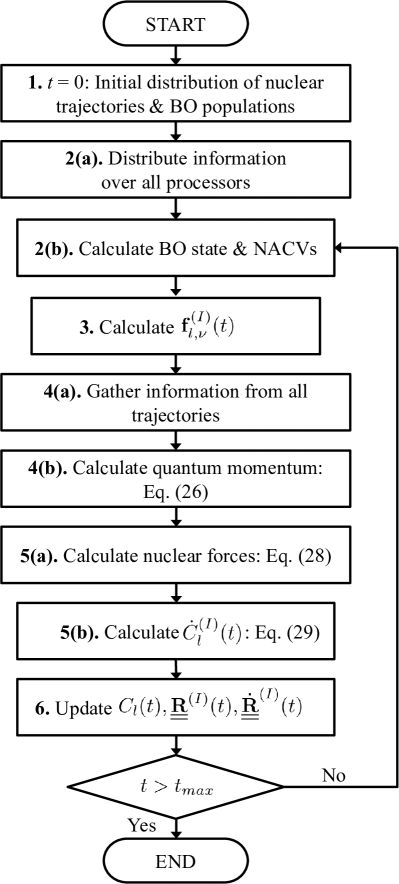
Figure 2: Flowchart describing the numerical implementation of the CT-MQC.

IV Numerical tests

Numerical results will be presented for one-dimensional model systems Tully (1990); Subotnik and Shenvi (2011a) that have nowadays become standard tests for any new quantum-classical approach to deal with non-adiabatic problems. Results of the CT-MQC are compared not only with an exact wave packet propagation scheme, but also with other quantum-classical approaches, namely Ehrenfest Ehrenfest (1927); Tully (1998); Drukker (1999), TSH Tully (1990); Tully and Preston (1971); Kohen et al. (1998) and independent-trajectory MQC Abedi et al. (2014); Agostini et al. (2014) (the zero-th order version of the algorithm proposed here). It will be clear from the results that the use of coupled trajectories, rather than independent trajectories, which all approaches but CT-MQC are based on, is indeed the key to electronic decoherence in non-adiabatic processes.

The models discussed below are (a) single avoided crossing, (b) dual avoided crossing, (c) extended coupling region with reflection, (d) double arch. The diabatic Hamiltonians are presented in Section SI.4 of the Supporting Information, while adiabatic PESs and NACVs are shown in Fig. 3.

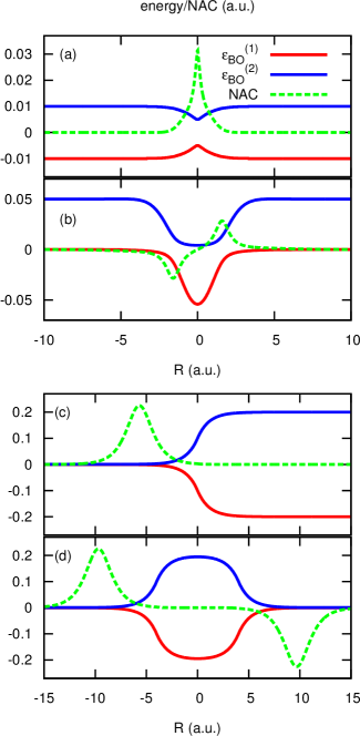
Figure 3: BOPESs (first, red line, and second, blue line) and NACVs (dashed green line) for the four model systems studied in the paper. The panels correspond to the problems of (a) single avoided crossing, (b) dual avoided crossing, (c) extended coupling region with reflection and (d) double arch. In panel (a) the curve representing the NACV has been reduced 50 times, in (b) 30 times. All quantities are shown in atomic units (a.u.).

In presenting the numerical results, particular attention is devoted to decoherence. In order to quantify decoherence, we use as indicator

$$\left|\rho_{12}(t)\right|^{2}=\frac{1}{N_{traj}}\sum_{I=1}^{N_{traj}}\left|C_{1}^{(I)}(t)\right|^{2}\left|C_{2}^{(I)}(t)\right|^{2},$$ (30)

which is an average over the trajectories of the (squared moduli of the) off-diagonal elements of the electronic density matrix in the adiabatic basis. The corresponding quantum mechanical quantity is

$$\left|\rho_{12}(t)\right|^{2}=\int d{\underline{\underline{\bf R}}}\,\left|C_{1}\left({\underline{\underline{\bf R}}},t\right)\right|^{2}\left|C_{2}\left({\underline{\underline{\bf R}}},t\right)\right|^{2}\left|\chi\left({\underline{\underline{\bf R}}},t\right)\right|^{2},$$ (31)

as proven in Section SI.4 of the Supporting Information.

IV.1 (a) - Single avoided crossing

A Gaussian wave packet is prepared on the lower adiabatic surface and launched from the far negative region with positive initial momentum towards the avoided crossing. Two values of the mean momentum are shown in the figures below, namely $\hbar k_{0}=10$ a.u. and $\hbar k_{0}=25$ a.u.

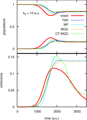
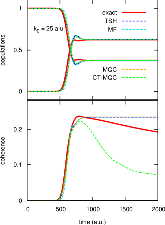
Figure 4: (Left) Upper panel: populations of the BO states as functions of time, computed via exact wave packet dynamics (red) and via the approximate schemes, TSH (blue), Ehrenfest MF (cyan), MQC (orange) and CT-MQC (green), for model (a). Lower panel: indicator of decoherence as function of time. The color code is the same as in the upper panel. The results are shown for model (a) using the value $\hbar k_{0}=10$ a.u. for the initial momentum. (Right) Same as in the left panels but for the value $\hbar k_{0}=25$ a.u. of the initial momentum.

We have computed the populations of the adiabatic states as functions of time (upper panels in Fig. 4), along with the indicator for the decoherence (lower panels in Fig. 4), given in Eq. (30). Fig. 4 shows those quantities for the low initial momentum (left) and for the high initial momentum (right). Numerical results are shown for exact wave packet propagation (red lines), TSH (blue lines), Ehrenfest dynamics (mean field, MF, cyan line), MQC (the independent trajectory version of the algorithm proposed here, orange) and CT-MQC (based on Eqs. (28) and (29), green lines). While all methods correctly predicted the electronic population after the passage through the avoided crossing, only the CT-MQC scheme is able to qualitatively account for electronic decoherence effects. CT-MQC results are not in perfect agreement with the exact ones, but indeed the algorithm captures a trend that is completely missed by the other methods.

As we have derived the CT-MQC scheme from the exact factorization, we have access to the time-dependent potentials of the theory, i.e. the TDPES and the TDVP. In Fig. 5 (left panels) we report the gauge-invariant part of the TDPES (red line), $\epsilon_{GI}$ in the figures, and we compare it with the same quantity computed with the CT-MQC procedure (blue dots), $\epsilon_{0}^{(I)}$ in the figures, for both initial momenta at a given time-step as indicated in the figure.

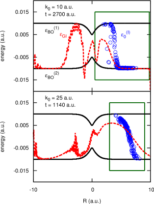
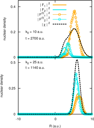
Figure 5: (Left) Snapshots (at time $t=2700$ a.u. for the low initial momentum $\hbar k_{0}=10$ a.u., upper panel, and at time $t=1140$ a.u. for the high initial momentum $\hbar k_{0}=25$ a.u., lower panel) of the gauge-invariant part of the TDPES ($\epsilon_{GI}$), shown as red lines for model (a). The black lines represent the BO surfaces, $\epsilon_{BO}^{(1)}$ and $\epsilon_{BO}^{(2)}$. The blue dots are the quantum-classical approximation to the potential. The regions highlighted in the green boxes are the regions where the calculation of the TDPES is reliable, since the nuclear density is different from zero. Outside this region the density is (numerically) zero and the results are affected by numerical noise. (Right) Snapshots at the same time-steps indicated in the left panel of the nuclear density (black lines) and of the BO-projected densities ($|F_{1}|^{2}$ orange lines and $|F_{2}|^{2}$ cyan lines) for the two initial momenta (upper panel $\hbar k_{0}=10$ a.u. and lower panel $\hbar k_{0}=25$ a.u.). The colored dots represent the quantum-classical approximation of the BO-projectes densities.

The gauge-invariant part of the TDPES is given by the first two terms in the definition (5) of $\epsilon({\underline{\underline{\bf R}}},t)$, whose approximation in the quantum-classical case is simply the first term on the right-hand-side of Eq. (10). In Fig. 5, the adiabatic PESs are shown for reference as black lines. If we observe the shape of the TDPES and of its approximation highlighted by the box (region where the nuclear density is significantly different from zero, thus it allows for the calculation of the TDPES), we see that the steps are reproduced very well in the quantum-classical picture. Since the CT-MQC correctly captures the shape of the potential, the nuclear density and the BO-projected densities are well reproduced. This is shown in the right panels in Fig. 5, for both initial momenta and at the same time-steps indicated in the left panels. Here, the nuclear density is indicated in black, while the BO-projected densities $|F_{l}|^{2}$ with $l=1,2$, are indicated as colored lines (exact) and dots (CT-MQC).

It is important to notice that the quantity shown in Fig. 5, the gauge-invariant part of the TDPES, is the only meaningful quantity that can be compared with exact results. For instance, the TDVP, being a gauge-dependent potential, is different if different gauges are used within the exact factorization. In particular, in the exact case we have chosen to work in a gauge where the TDVP is always zero, while quantum-classical calculations are performed in the gauge defined by Eq. (9).

IV.2 (b) - Dual avoided crossing

The same initial conditions as for model (a) have been used for the dual avoided crossing, with $\hbar k_{0}=16$ a.u. and $\hbar k_{0}=30$ a.u. chosen as initial momenta. We notice in Fig. 6 that for low initial momentum the new algorithm is not able to correctly reproduce the final population of the adiabatic states after the two consecutive passages thorough the avoided crossings.

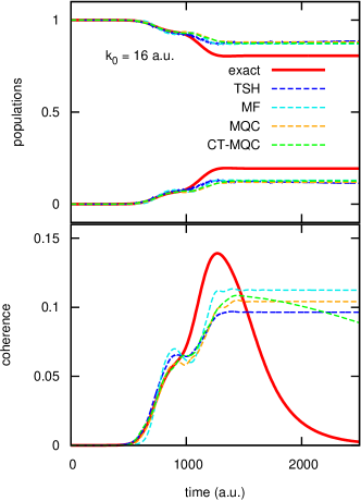
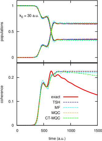
Figure 6: (Left) Same as in Fig. 4 but for the model system (b) and for the value $\hbar k_{0}=16$ a.u. of the initial momentum. (Right) Same as in the left panel but for the value $\hbar k_{0}=30$ a.u. of the initial momentum.

For both momentum values, also decoherence is not correctly captured. We observe however a slight deviation of the CT-MQC results from the other (independent-trajectory) algorithms, since the green lines in the lower panels of Fig. 6 decay, but such decay is much slower than the expected behavior predicted by quantum mechanical results (red lines). In model (b) the avoided crossing regions are very close to each other. Therefore, the overall effect of NACVs is not localized in space, in constrast to what we have assumed in deriving Eq. (17). Furthermore, in the fifth approximation introduced above we have assumed that population exchange due to the NACVs and decoherence due to the quantum momentum are separated effects. Model (b), at low initial momentum, is a situation where this does not happen. The nuclear wave packet encounters the first avoided crossing and branches on different surfaces. Then decoherence starts appearing, but at this point the wave packets cross the second non-adiabatic region. The combined effect of NACVs and quantum momentum is thus not completely taken into account by the CT-MQC equations. It follows that the CT-MQC scheme does not capture correctly the adiabatic populations. However, we do capture the separation of the nuclear wave packet on different BO surfaces, as described below.

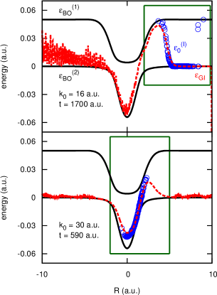
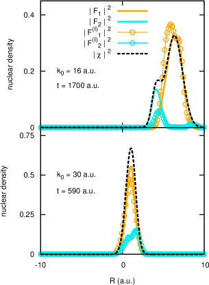
Figure 7: (Left) Same as in Fig. 5, but the snapshots are shown at time $t=1700$ a.u. for the low initial momentum $\hbar k_{0}=16$ a.u. (upper panel) and at time $t=590$ a.u. for the high initial momentum $\hbar k_{0}=30$ a.u. (lower panel), for model (b).

Fig. 7 shows the gauge-invariant part of the TDPES (left panels) and the nuclear densities (right panels) for both initial momenta. Despite the deviations of quantum-classical results from exact results for the electronic properties, the time-dependent potential and, consequently, the nuclear dynamics are correctly reproduced in the approximate picture.

IV.3 (c) - Extended coupling region with reflection

This and the following model systems represent critical tests of decoherence. In both cases, the structure of the adiabatic surfaces, one with a well and one with a barrier, is responsible for yielding a high probability of reflection, especially at low initial momenta. In the case when one branch of the nuclear wave packet is reflected and the other is transmitted, the two wave packets propagate along diverging paths in nuclear space thus they lose memory of each other. This effect can be accounted for in a coupled-trajectory picture but not if independent trajectories are used, since the electronic equations are propagated fully coherently along each (independent from each other) trajectory.

Figs. 8 and 9 show results for two values of the initial momentum, namely $\hbar k_{0}=10$ a.u. and $\hbar k_{0}=30$ a.u., for model system (c), in analogy to what has been presented in the previous examples. In particular, we notice that for the low initial momentum, the CT-MQC is able to reproduce the time-dependence of the adiabatic populations in very close agreement with exact results, yielding a better agreement than TSH. The population exchange occurring after 4000 a.u. (upper left panel of Fig. 8) is not captured by Ehrenfest and the MQC algorithm, since these approaches cannot reproduce nuclear dynamics along diverging paths, as already discussed in previous work Abedi et al. (2014); Agostini et al. (2014). Such second non-adiabatic event is observed when the reflected wave packet crosses for the second time the extended coupling region. This channel is not accessible in Ehrenfest and MQC calculations.

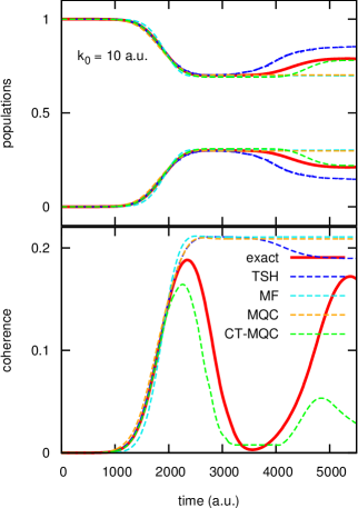
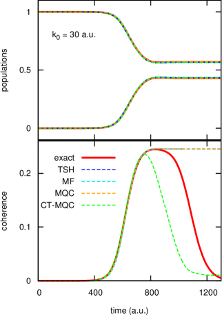
Figure 8: (Left) Same as in Fig. 4 but for the model system (c) and for the value $\hbar k_{0}=10$ a.u. of the initial momentum. (Right) Same as in the left panel but for the value $\hbar k_{0}=30$ a.u. of the initial momentum.

The CT-MQC yields decoherence effects in strikingly good agreement with exact results. The electronic equations in TSH and Ehrenfest are given by the first two terms on the right-hand-side of Eq. (29) and, as shown in the lower panels in Fig. 8, those procedures completely miss the decay of coherence predicted by wave packet propagation. The additional term in Eq. (29) containing the quantum momentum is sufficient to correct for this effect.

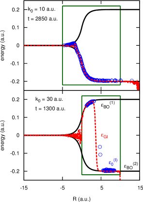
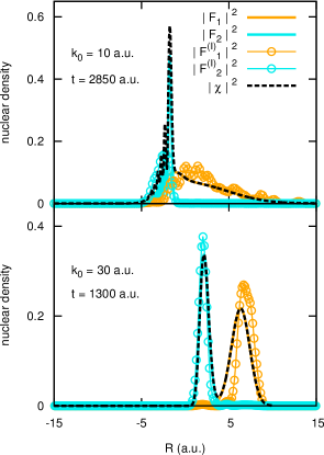
Figure 9: Same as in Fig. 5, but the snapshots are shown at time $t=2850$ a.u. for the low initial momentum $\hbar k_{0}=10$ a.u. (upper panel) and at time $t=1300$ a.u. for the high initial momentum $\hbar k_{0}=30$ a.u. (lower panel), for model (c).

As expected, also the TDPES and the nuclear densities are very well reproduced by the CT-MQC procedure, when compared to exact calculations.

IV.4 (d) - Double arch

The double arch model has been introduced Subotnik and Shenvi (2011a) to enhance decoherence effects on electronic dynamics. For low initial momenta, this model is similar to model (c), since the nuclear wave packet is partially transmitted and partially reflected. After the splitting though, both components go a second time through a region of extended coupling, thus they experience once again a non-adiabatic event. We observe this behavior when $\hbar k_{0}=20$ a.u. is chosen as initial momentum. By contrast, at higher initial momentum, i.e. $\hbar k_{0}=40$ a.u., both wave packets are transmitted and propagate in the positive region until they recombine. Capturing correctly the dynamics of the recombination is what makes this model system a challenge for the inclusion of decoherence effects. After the two transmitted wave packets propagate independently of each other on the two (very different) adiabatic surfaces, they recombine with some time-delay, therefore decoherence should first decay and then reappear as consequence of the recombination.

Fig. 10 shows that all features related to decoherence discussed above are indeed captured by the CT-MQC algorithm, in very good agreement with exact results, and are completely missed by all other methods. At high initial momentum, only TSH and CT-MQC are able to reproduce the electronic population after the second non-adiabatic event after 1000 a.u. (as shown in Fig. 10 upper right panel), but only CT-MQC results are in perfect agreement with exact results.

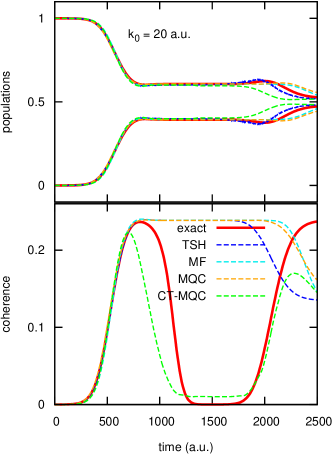
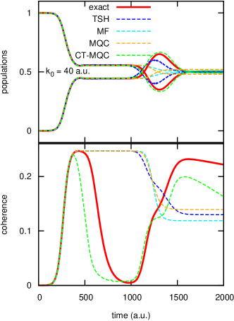
Figure 10: (Left) Same as in Fig. 4 but for the model system (d) and for the value $\hbar k_{0}=20$ a.u. of the initial momentum. (Right) Same as in the left panel but for the value $\hbar k_{0}=40$ a.u. of the initial momentum.

The non-adiabatic process represented in model (d), as well as in model (c), presents very different BO surfaces. Therefore, the correct nuclear dynamics cannot be captured by methods, such as Ehrenfest and MQC, relying on a single potential energy surface which is (or is close to) an average potential. Such an average potential cannot reproduce the very different forces that are experienced by the nuclear trajectories in different regions of space. By contrast, the single TDPES from the exact factorization is able to capture very different shapes because of the steps Abedi et al. (2013a) that bridge piecewise adiabatic shapes. At a given time, depending on where the classical trajectory is located, it can experience very different forces.

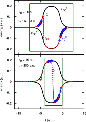
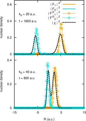
Figure 11: (Left) Same as in Fig. 5, but the snapshots are shown at time $t=1600$ a.u. for the low initial momentum $\hbar k_{0}=20$ a.u. (upper panel) and at time $t=800$ a.u. for the high initial momentum $\hbar k_{0}=40$ a.u. (lower panel), for model (d).

This is clearly shown in Fig. 11.

IV.5 Dependence on the initial momentum

It is interesting to investigate the dependence of the final transmission/reflection probabilities on the initial momentum of the nuclear nuclear wave packet for the four model systems studied here. Similar studies have been already reported in the literature Tully (1990); Subotnik and Shenvi (2011a); Shenvi et al. (2011a); Curchod and Tavernelli (2013), focussing on the performance of TSH in comparison to quantum propagation techniques. Here, we will only benchmark the CT-MQC algorithm against exact results. We refer to the above-mentioned references for TSH results, since we are considering the same initial conditions used there. Moreover, we will not show the results for Ehrenfest and for the independent-trajectory version of the MQC algorithm derived from the exact factorization. The reason is that neither method is capable of following the evolution of nuclear wave packets along diverging paths (at least with the initial conditions chosen below), as we have previously discussed Agostini et al. (2014).

In all cases, the initial variance of the nuclear wave packet is chosen as $\sigma=20/(\hbar k_{0})$. The initial conditions for the classical trajectories are sampled in position space from a Gaussian distribution with variance $\sigma$, while the same momentum, $\hbar k_{0}$, is assigned to all trajectories. For model (d), we have only chosen large values of $\hbar k_{0}$, since for lower values model (d) is similar to model (c).

Figure 12 shows a good agreement between exact and quantum-classical results for models (a), (c) and (d). As expected from the results reported for model (b) in Fig. 6 at low initial momentum, the CT-MQC is not able to reproduce the final probabilities up to $\hbar k_{0}=20$ a.u., but it improves at higher values. Still, it slightly underestimates the non-adiabatic population exchange up to a value of $\hbar k_{0}=26$ a.u. of the initial momentum.

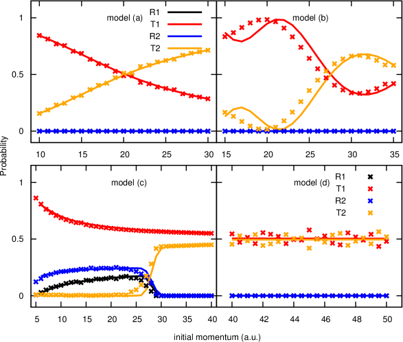
Figure 12: Dependence of the final transmission/reflection probabilities on the initial momentum $\hbar k_{0}$. Transmission probabilities at the final times on the lower and upper surfaces are indicated as T1 and T2, respectively; similarly, the reflection probabilities are indicated as R1 and R2. The lines refer to exact calculations, the dots to the results of the CT-MQC algorithm. The initial variance of the nuclear wave packet is chosen as $\sigma=20/(\hbar k_{0})$.

Also, it is worth noting that the (well-known) unphysical oscillations in model (c), observed for the reflection channels in TSH Tully (1990); Subotnik and Shenvi (2011a), are not present in our CT-MQC results. In TSH, the oscillations appear when the initial momenta are not sampled from a distribution Subotnik and Shenvi (2011b) but a fixed value of $\hbar k_{0}$ is assigned to all trajectories, as done here. They are due to the phase coherence between the first and the second passage of the wave packet through the region of extended coupling. The CT-MQC algorithm correctly eliminates any sign of spurious coherence, that is in agreement with quantum mechanical results.

In model (d), the final probabilities shown in Fig. 12 slightly oscillate around the exact value, but the deviation is not larger than 10%. The model has been initially introduced Subotnik and Shenvi (2011a) to enhance the over-coherence problem of TSH and to investigate possible correction strategies. Some studies have been reported Subotnik and Shenvi (2011a); Curchod and Tavernelli (2013) where the initial width of the nuclear wave packet is larger than the cases above, i.e. $\sigma=100/(\hbar k_{0})$, which yields a very localized wave packet in momentum space. We have simulated also this situation, following the same protocol as described above for sampling classical initial conditions, for the same range of $\hbar k_{0}$. In a recent work Curchod and Tavernelli (2013), Curchod and Tavernelli have shown that TSH (i) is not able to reproduce the oscillations in the transmitted probabilities, if the initial positions and momenta of the classical trajectories are sampled from Gaussian distributions, and (ii) captures the oscillatory behavior of the transmitted probabilities (even though not the correct one), if the same positions and momenta are chosen for all trajectories, which will then differ from each other at later times, due to the stochastic jumps. In the CT-MQC algorithm, if option (ii) is chosen, all trajectories will follow the same path and no splitting will be observed. This is intrinsic of the deterministic nature of the algorithm. Therefore, we chose the option to sample the initial positions from a Gaussian distribution and we assigned the same initial momentum $\hbar k_{0}$ to all trajectories. As it can be seen in Fig. 13, the CT-MQC algorithm is not able to match the exact results.

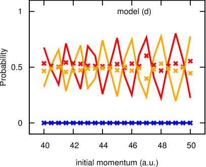
Figure 13: Dependence of the final transmission/reflection probabilities on the initial momentum $\hbar k_{0}$ for model (d). The initial variance of the nuclear wave packet is chosen as $\sigma=100/(\hbar k_{0})$.

Here, we would like to emphasise that this a very pathological situation, introduced to exaggerate the over-coherence issue of TSH. Further studies and more accurate approximations might be necessary to cure this problem in CT-MQC.

V Conclusions

We have presented a detailed derivation of the CT-MQC scheme Min et al. (2015) to non-adiabatic dynamics starting from the exact factorization of the electron-nuclear wave function. When compared to the independent-trajectory MQC Abedi et al. (2014); Agostini et al. (2014), the CT-MQC offers a clear improvement, since the new method is now able to correctly reproduce electronic decoherence and the spatial splitting of the nuclear wave packet, which in turn is connected to the ability of reproducing the steps Abedi et al. (2013a); Agostini et al. (2013, 2015a) in the gauge-invariant part of the TDPES. In the proposed scheme, the classical trajectories are indirectly coupled through the electronic equation. This feature is therefore different from the direct interaction among trajectories provided by the quantum potential in Bohmian dynamics.

Two key features have been included here, that go beyond our previous lowest order algorithm, (i) the quantum momentum appears in the electronic equation, when considering $\mathcal{O}(\hbar)$ terms in the expression of the ENCO depending on the nuclear wave function, and (ii) the spatial dependence of the coefficients in the Born-Huang expansion of the electronic wave function has been taken into account to leading order, while it was completely neglected in our previous work. In the new picture we have been able to distinguish the two effects induced by nuclear motion on electronic dynamics, populations dynamics and decoherence. On the one hand, non-adiabatic transitions are induced by the nuclear momentum, the zero-th order term of the $\hbar$-expansion, which couples to the NACVs. On the other hand, decoherence effects are controlled by the quantum momentum, the first-order term of the $\hbar$-expansion, which is an imaginary correction to the nuclear momentum in the ENCO. In turn, the effect of the electrons on nuclear dynamics is represented by the TDPES and the TDVP. As discussed in previous work Abedi et al. (2013a); Agostini et al. (2013, 2015a), being able to reproduce their features, such as the steps, in an approximate scheme results in the correct description of the nuclear wave packet behavior.

In this paper the analytical development of the algorithm is supported by tests performed on some model systems Tully (1990); Subotnik and Shenvi (2011a) which are typical examples of electronic non-adiabatic processes. The comparison of the CT-MQC results with wave packet dynamics has shown that indeed we are able to predict the correct physical picture, capturing the dynamical details of both electronic and nuclear subsystems. Moreover, we have proved that the new algorithm, being a coupled-trajectory scheme, is able to overcome the issues that are encountered when other methods, based on an independent-trajectory picture, are employed.

Further developments are envisaged, mainly focusing on the application of the method to more realistic problems and on the semiclassical treatment of nuclear dynamics, possibly allowing the treatment of nuclear interference effects.

Supporting Information Available

Section SI.1 of the Supporting Information introduces the exact factorization framework, recalling the general theory and the equations that are the starting point for the approximations developed in the main text.

Section SI.2 justifies the approximations leading to Eq. (17) by using semiclassical arguments. Moreover, we recall there the analysis of the coefficients $|C_{l}({\underline{\underline{\bf R}}},t)|$ of the Born-Huang expansion of the electronic wave function that we presented in previous work Abedi et al. (2013a).

The equations to compute the quantum momentum in a multi-level system are derived in Section SI.3 of the Supporting Information and are presented as a generalization of the two-level case discussed in the main text.

Finally, Section SI.4 gives the computational details for the numerical tests.

This information is available free of charge via the Internet at http://pubs.acs.org/.

Table of Contents graphic

References

- Polli et al. (2010) D. Polli, P. Altoè, O. Weingart, K. M. Spillane, C. Manzoni, D. Brida, G. Tomasello, G. Orlandi, P. Kukura, R. A. Mathies, M. Garavelli, and G. Cerullo, Nature 467, 440 (2010).
- Hayashi et al. (2009) S. Hayashi, E. Tajkhorshid, and K. Schulten, Biophys. J. 416, 403 (2009).
- Chung et al. (2012) W. C. Chung, S. Nanbu, and T. Ishida, J. Phys. Chem. B 116, 8009 (2012).
- Tapavicza et al. (2011) E. Tapavicza, A. M. Meyer, and F. Furche, Phys. Chem. Chem. Phys. 13, 20986 (2011).
- Brixner et al. (2005) T. Brixner, J. Stenger, H. M. Vaswani, M. Cho, R. E. Blankenship, and G. R. Fleming, Nature 434, 625 (2005).
- Rozzi et al. (2013) C. A. Rozzi, S. M. Falke, N. Spallanzani, A. Rubio, E. Molinari, D. Brida, M. Maiuri, G. Cerullo, H. Schramm, J. Christoffers, and C. Lienau, Nature Comm. 4, 1602 (2013).
- Silva (2013) C. Silva, Nature Mat. 12, 5 (2013).
- Jailaubekov et al. (2013) A. E. Jailaubekov, A. P. Willard, J. R. Tritsch, W.-L. Chan, N. Sai, R. Gearba, L. G. Kaake, K. J. Williams, K. Leung, P. J. Rossky, and X.-Y. Zhu, Nature Mat. 12, 66 (2013).
- Repp et al. (2010) J. Repp, P. Liljeroth, and G. Meyer, Nature Phys. 6, 975 (2010).
- Reckermann et al. (2010) F. Reckermann, J. Splettstoesser, and M. R. Wegewijs, Phys. Rev. Lett. 104, 226803 (2010).
- Härtle et al. (2011) R. Härtle, M. Butzin, O. Rubio-Pons, and M. Thoss, Phys. Rev. Lett. 107, 046802 (2011).
- Dundas et al. (2009) D. Dundas, E. J. McEniry, and T. N. Todorov, Nature Nano. 4, 99 (2009).
- Martínez and Levine (1996) T. J. Martínez and R. D. Levine, Chem. Phys. Lett. 259, 252 (1996).
- Martínez et al. (1996) T. J. Martínez, M. Ben-Nun, and R. D. Levine, J. Phys. Chem. 100, 7884 (1996).
- Martínez (2006) T. J. Martínez, Acc. Chem. Res. 39, 119 (2006).
- Meyer et al. (1990) H.-D. Meyer, U. Manthe, and L. S. Cederbaum, Chem. Phys. Lett. 165, 73 (1990).
- Burghardt et al. (1999) I. Burghardt, H.-D. Meyer, and L. S. Cederbaum, J. Chem. Phys. 111, 2927 (1999).
- Thoss et al. (2004) M. Thoss, W. Domcke, and H. Wang, Chem. Phys. 296, 217 (2004).
- Curchod et al. (2011) B. F. E. Curchod, I. Tavernelli, and U. Rothlisberger, Phys. Chem. Chem. Phys. 13, 3231 (2011).
- Tavernelli (2013) I. Tavernelli, Phys. Rev. A 87, 042501 (2013).
- Albareda et al. (2014) G. Albareda, H. Appel, I. Franco, A. Abedi, and A. Rubio, Phys. Rev. Lett. 113, 083003 (2014).
- Albareda et al. (2015) G. Albareda, J. M. Bofill, I. Tavernelli, F. Huarte-Larrañaga, F. Illas, and A. Rubio, J. Phys. Chem. Lett. 6, 1529 (2015).
- Wyatt et al. (2001) R. E. Wyatt, C. L. Lopreore, and G. Parlant, J. Chem. Phys. 114, 5113 (2001).
- Lopreore and Wyatt (2002) C. L. Lopreore and R. E. Wyatt, J. Chem. Phys. 116, 1228 (2002).
- Poirier and Parlant (2007) B. Poirier and G. Parlant, J. Phys. Chem. A 111, 10400 (2007).
- Pechukas (1969a) P. Pechukas, Phys. Rev. 181, 166 (1969a).
- Pechukas (1969b) P. Pechukas, Phys. Rev. 181, 174 (1969b).
- Ehrenfest (1927) P. Ehrenfest, Zeitschrift für Physik 45, 455 (1927).
- Shalashilin (2009) D. V. Shalashilin, J. Chem. Phys. 130, 244101 (2009).
- Tully and Preston (1971) J. C. Tully and R. K. Preston, J. Chem. Phys. 55, 562 (1971).
- Tully (1990) J. C. Tully, J. Chem. Phys. 93, 1061 (1990).
- Kohen et al. (1998) D. Kohen, F. H. Stillinger, and J. C. Tully, J. Chem. Phys. 109, 4713 (1998).
- Burant and Tully (2000) J. C. Burant and J. C. Tully, J. Chem. Phys. 112, 6097 (2000).
- Prezhdo and Brooksby (2001) O. V. Prezhdo and C. Brooksby, Phys. Rev. Lett. 86, 3215 (2001).
- Shenvi et al. (2011a) N. Shenvi, J. E. Subotnik, and W. Yang, J. Chem. Phys. 134, 144102 (2011a).
- Subotnik et al. (2013) J. E. Subotnik, W. Ouyang, and B. R. Landry, J. Chem. Phys. 139, 214107 (2013).
- Kapral and Ciccotti (1999) R. Kapral and G. Ciccotti, J. Chem.Phys. 110, 8916 (1999).
- Kapral (2006) R. Kapral, Annu. Rev. Phys. Chem. 57, 129 (2006).
- Agostini et al. (2007) F. Agostini, S. Caprara, and G. Ciccotti, Europhys. Lett. 78, 30001 (2007).
- Shi and Geva (2004) Q. Shi and E. Geva, J. Chem. Phys. 121, 3393 (2004).
- Horenko et al. (2001) I. Horenko, B. Schmidt, and C. Schütte, J. Chem. Phys. 115, 5733 (2001).
- Martens and Fang (1997) C. C. Martens and J.-Y. Fang, J. Chem. Phys. 106, 4918 (1997).
- Bonella and Coker (2001) S. Bonella and D. Coker, Chem. Phys. 268, 189 (2001).
- Huo and Coker (2012) P. Huo and D. F. Coker, J. Chem. Phys. 137, 22A535 (2012).
- Sun and Miller (1997) X. Sun and W. H. Miller, J. Chem. Phys. 106, 916 (1997).
- Stock and Thoss (1997) G. Stock and M. Thoss, Phys. Rev. Lett. 78, 578 (1997).
- Ananth et al. (2007) N. Ananth, C. Venkataraman, and W. H. Miller, J. Chem. Phys. 127, 084114 (2007).
- Miller (2009) W. H. Miller, J. Phys. Chem. A 113, 1405 (2009).
- Thoss and Wang (2004) M. Thoss and H. Wang, Annu. Rev. Phys. Chem. 55, 299 (2004).
- Herman (1994) M. F. Herman, Ann. Rev. Phys. Chem. 45, 83 (1994).
- Wu and Herman (2005) Y. Wu and M. F. Herman, J. Chem. Phys. 123, 144106 (2005).
- Jasper et al. (2004) A. W. Jasper, C. Zhu, S. Nangia, and D. G. Truhlar, Faraday Discuss. 127, 1 (2004).
- Jasper et al. (2006) A. W. Jasper, S. Nangia, C. Zhu, and D. G. Truhlar, Acc. Chem. Res. 39, 101 (2006).
- Bousquet et al. (2011) D. Bousquet, K. H. Hughes, D. A. Micha, and I. Burghardt, J. Chem. Phys. 134, 064116 (2011).
- Jang (2012) S. Jang, J. Chem. Phys. 137, 22A536 (2012).
- Zimmermann and Vanicek (2012) T. Zimmermann and J. Vanicek, J. Chem. Phys. 136, 094106 (2012).
- Hanasaki and Takatsuka (2010) K. Hanasaki and K. Takatsuka, Phys. Rev. A 81, 052514 (2010).
- Bonella and Coker (2005) S. Bonella and D. F. Coker, J. Chem. Phys. 122, 194102 (2005).
- Doltsinis and Marx (2002) N. L. Doltsinis and D. Marx, Phys. Rev. Lett. 88, 166402 (2002).
- Abedi et al. (2014) A. Abedi, F. Agostini, and E. K. U. Gross, Europhys. Lett. 106, 33001 (2014).
- Prezhdo and Rossky (1997) O. V. Prezhdo and P. J. Rossky, J. Chem. Phys. 107, 825 (1997).
- Zamstein and Tannor (2012) N. Zamstein and D. J. Tannor, J. Chem. Phys. 137, 22A518 (2012).
- Abedi et al. (2010) A. Abedi, N. T. Maitra, and E. K. U. Gross, Phys. Rev. Lett. 105, 123002 (2010).
- Abedi et al. (2012) A. Abedi, N. T. Maitra, and E. K. U. Gross, J. Chem. Phys. 137, 22A530 (2012).
- Min et al. (2015) S. K. Min, F. Agostini, and E. K. U. Gross, Phys. Rev. Lett. 115, 073001 (2015).
- Abedi et al. (2013a) A. Abedi, F. Agostini, Y. Suzuki, and E. K. U. Gross, Phys. Rev. Lett. 110, 263001 (2013a).
- Agostini et al. (2013) F. Agostini, A. Abedi, Y. Suzuki, and E. K. U. Gross, Mol. Phys. 111, 3625 (2013).
- Agostini et al. (2015a) F. Agostini, A. Abedi, Y. Suzuki, S. K. Min, N. T. Maitra, and E. K. U. Gross, J. Chem. Phys. 142, 084303 (2015a).
- Agostini et al. (2015b) F. Agostini, S. K. Min, and E. K. U. Gross, Ann. Phys. 527, 546 (2015b).
- Agostini et al. (2014) F. Agostini, A. Abedi, and E. K. U. Gross, J. Chem. Phys. 141, 214101 (2014).
- Shenvi and Yang (2012) N. Shenvi and W. Yang, J. Chem. Phys. 137, 22A528 (2012).
- Subotnik and Shenvi (2011a) J. E. Subotnik and N. Shenvi, J. Chem. Phys. 134, 024105 (2011a).
- Shenvi et al. (2011b) N. Shenvi, J. E. Subotnik, and W. Yang, J. Chem. Phys. 134, 144102 (2011b).
- Subotnik (2011) J. E. Subotnik, J. Phys. Chem. A 115, 12083 (2011).
- Akimov et al. (2014) A. V. Akimov, R. Long, and O. V. Prezhdo, J. Chem. Phys. 140, 194107 (2014).
- Nelson et al. (2013) T. Nelson, S. Fernandez-Alberti, A. E. Roitberg, and S. Tretiak, J. Chem. Phys. 138, 224111 (2013).
- Prezhdo (1999) O. V. Prezhdo, J. Chem. Phys. 111, 8366 (1999).
- Bittner and Rossky (1995) E. R. Bittner and P. J. Rossky, J. Chem. Phys. 103, 8130 (1995).
- Bittner and Rossky (1997) E. R. Bittner and P. J. Rossky, J. Chem. Phys. 107, 8611 (1997).
- Cheng et al. (2008) S. C. Cheng, C. Zhu, K. K. Liang, S. H. Lin, and D. G. Truhlar, J. Chem. Phys. 129, 024112 (2008).
- Bedard-Hearn et al. (2005) M. J. Bedard-Hearn, R. E. Larsen, and B. J. Schwartz, J. Chem. Phys. 123, 234106 (2005).
- Granucci and Persico (2007) G. Granucci and M. Persico, J. Chem. Phys. 126, 134114 (2007).
- Granucci et al. (2010) G. Granucci, M. Persico, and A. Zoccante, J. Chem. Phys. 133, 134111 (2010).
- Bajo et al. (2014) J. J. Bajo, G. Granucci, and M. Persico, J. Comput. Chem. 140, 044113 (2014).
- Gidopoulos and Gross (2014) N. I. Gidopoulos and E. K. U. Gross, Phil. Trans. R. Soc. A 372, 20130059 (2014).
- Min et al. (2014) S. K. Min, A. Abedi, K. S. Kim, and E. K. U. Gross, Phys. Rev. Lett. 113, 263004 (2014).
- (87) R. Requist, F. Tandetzky, and E. K. U. Gross, arXiv:1506.09193v3 [physics.chem-ph] .
- Suzuki et al. (2014) Y. Suzuki, A. Abedi, N. T. Maitra, K. Yamashita, and E. K. U. Gross, Phys. Rev. A 89, 040501(R) (2014).
- Suzuki et al. (2015) Y. Suzuki, A. Abedi, N. T. Maitra, and E. K. U. Gross, Phys. Chem. Chem. Phys. 17, 29271 (2015).
- Khosravi et al. (2015) E. Khosravi, A. Abedi, and N. T. Maitra, Phys. Rev. Lett. 115, 263002 (2015).
- Schild et al. (2016) A. Schild, F. Agostini, and E. K. U. Gross, Accepted in J. Phys. Chem. A (2016), DOI: 10.1021/acs.jpca.5b12657.
- Frenkel (1934) J. Frenkel, “Wave mechanics: Advanced general theory,” (1934) p. 253, Clarendon, Oxford ed.
- Alonso et al. (2013) J. L. Alonso, J. Clemente-Gallardo, P. Echeniche-Robba, and J. A. Jover-Galtier, J. Chem. Phys. 139, 087101 (2013).
- Abedi et al. (2013b) A. Abedi, N. T. Maitra, and E. K. U. Gross, J. Chem. Phys. 139, 087102 (2013b).
- van Vleck (1928) J. H. van Vleck, Proc. Natl. Acad. Sci. USA 14, 178 (1928).
- Scherrer et al. (2015) A. Scherrer, F. Agostini, D. Sebastiani, E. K. U. Gross, and R. Vuilleumier, J. Chem. Phys. 143, 074106 (2015).
- Tapavicza et al. (2007) E. Tapavicza, I. Tavernelli, and U. Rothlisberger, Phys. Rev. Lett. 107, 621 (2007).
- Worth et al. (2003) G. A. Worth, P. Hunt, and M. A. Robb, J. Phys. Chem. A 26, 613 (2003).
- Burghardt et al. (2004) I. Burghardt, L. S. Cederbaum, and J. T. Hynes, Faraday Discuss. 127, 395 (2004).
- Garashchuk and Rassolov (2003) S. Garashchuk and V. A. Rassolov, Chem. Phys. Lett. 376, 358 (2003).
- Curchod and Tavernelli (2013) B. F. E. Curchod and I. Tavernelli, J. Chem. Phys. 138, 184112 (2013).
- Note (1) If the squared moduli of the coefficients are multiplied by the nuclear density and integrated over nuclear space, as proven in Section SI.1 of the Supporting Information.
- Tully (1998) J. C. Tully, Faraday Discuss. 110, 407 (1998).
- Drukker (1999) K. Drukker, J. Comput. Phys. 153, 225 (1999).
- Subotnik and Shenvi (2011b) J. E. Subotnik and N. Shenvi, J. Chem. Phys. 134, 244114 (2011b).