Reducing Parallel Communication in Algebraic Multigrid through Sparsification

Abstract

Algebraic multigrid (AMG) is an $\mathcal{O}(n)$ solution process for many large sparse linear systems. A hierarchy of progressively coarser grids is constructed that utilize complementary relaxation and interpolation operators. High-energy error is reduced by relaxation, while low-energy error is mapped to coarse-grids and reduced there. However, large parallel communication costs often limit parallel scalability. As the multigrid hierarchy is formed, each coarse matrix is formed through a triple matrix product. The resulting coarse-grids often have significantly more nonzeros per row than the original fine-grid operator, thereby generating high parallel communication costs on coarse-levels. In this paper, we introduce a method that systematically removes entries in coarse-grid matrices after the hierarchy is formed, leading to an improved communication costs. We sparsify by removing weakly connected or unimportant entries in the matrix, leading to improved solve time. The main trade-off is that if the heuristic identifying unimportant entries is used too aggressively, then AMG convergence can suffer. To counteract this, the original hierarchy is retained, allowing entries to be reintroduced into the solver hierarchy if convergence is too slow. This enables a balance between communication cost and convergence, as necessary. In this paper we present new algorithms for reducing communication and present a number of computational experiments in support.

siscxxxxxxxx–x

1 Introduction

Algebraic multigrid (AMG) [16, 6, 17] is an $\mathcal{O}(n)$ linear solver. For standard discretizations of elliptic differential equations, AMG is remarkably fast [2, 22, 19]. We consider AMG as a solver for the symmetric, positive definite matrix problem

(1) $$Ax=b,$$

with $A\in\mathbb{R}^{n\times n}$ and $x,b\in\mathbb{R}^{n}$. AMG consists of two phases, a setup and a solve phase. The setup phase defines a sequence or hierarchy of $\ell_{\text{max}}$ coarse-grid and interpolation operators, $A_{1},\dots,A_{\ell_{\text{max}}}$ and $P_{0},\dots,P_{\ell_{\text{max}}-1}$ respectively. The solve phase iteratively improves the solution through relaxation and coarse-grid correction. The error not reduced by relaxation, called algebraically smooth, is transferred to cheaper coarser-levels and reduced there.

The focus of this paper is on the communication complexity of AMG in a distributed memory, parallel setting. To be clear, we refer to the communication complexity as the time cost of interprocessor communication, while referring to the computational complexity as the time cost of the floating point operations. The complexity or total complexity is then the cost of the algorithm, combining the communication and computational complexities.

Both the convergence and complexity of an algebraic multigrid method are controlled by the setup phase. Highly accurate interpolation, which yields a rapidly converging method, requires a slow rate of coarsening and often denser coarse operators. This large number of coarse-levels, as well as increased density, correlates with an increase in the amount of work required during a single iteration of the AMG solve phase. In contrast, sparser interpolation and fast coarsening reduce the cost of a single iteration of AMG cycle, but often lead to a deterioration in convergence [22, 19]. Therefore, there is a trade-off between per-iteration complexity and the resulting convergence factor.

The sparse matrices, $A_{1},\dots,A_{\ell_{\text{max}}}$, in the multigrid hierarchy are, by design, smaller in dimension, yet often decrease in sparsity. As an example of this, Table 1 shows the properties of a hierarchy for a 3D Poisson problem with a 7-point finite difference stencil on a $100\times 100\times 100$ grid. We see that as the problem size decreases on coarse-levels, the average number of nonzero entries per row increases. Here we denote by nnz the number of nonzero entries in the respective matrix. Figure 1 depicts this effect for this example, where we see that the density increases on lower levels in the hierarchy.

level	matrix size	nonzeros	nonzeros per row
$\ell$	$n$	nnz	$\nicefrac{{\textnormal{{nnz}}}}{{$n$}}$
0	$1\,000\,000$	$6\,940\,000$	$7$
1	$500\,000$	$9\,320\,600$	$19$
2	$83\,345$	$2\,775\,281$	$33$
3	$13\,265$	$745\,689$	$56$
4	$2207$	$208\,173$	$94$
5	$333$	$23\,843$	$72$

Table 1: Matrix properties using classical AMG for a 3D Poisson problem.

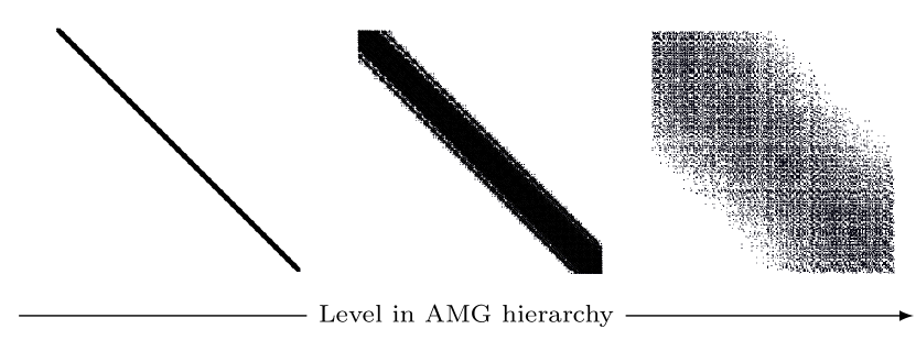
Fig. 1: Matrix sparsity pattern using classical AMG for three levels in the hierarchy: $\ell=0$, 3, 5. The full matrix properties are given in Table 1.

In parallel, the increase in density (decrease in sparsity) on coarse-levels correlates with an increase in parallel communication costs. Figure 2 shows this by plotting the time spent on each level in an AMG hierarchy during the solve phase. The time grows substantially on coarse-levels and this is almost completely due to increased communication costs from the decreasing sparsity. The time spent on smaller, coarse problems is much larger than the time spent working on the original, finest-level problem. The test problem is again the 3D Poisson problem, using the hypre [2] package with Falgout coarsening [7], extended classical modified interpolation, and hybrid symmetric Gauss-Seidel relaxation. This problem was run on 2048 processes with $10,000$ degrees-of-freedom per process.

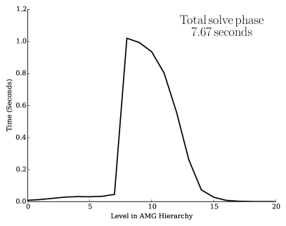
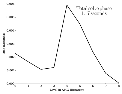
Fig. 2: Left: Time spent on each level of the hierarchy during a single iteration of classical parallel AMG for a 3D Poisson problem. Right: repeat experiment, but using aggressive HMIS coarsening. The total time is much lower; however, the qualitative feature of expensive coarse-levels remains.

In this paper we introduce a method for controlling the communication complexity in AMG. The method increases the sparsity of only coarse-grid operators ($A_{\ell}$, $\ell=1,\dots,\ell_{\text{max}}$) by eliminating entries in $A_{\ell}$ with no effect on interpolation operators ($P_{\ell}$, $\ell=0,\ldots,\ell_{\text{max}-1}$). This results in an improved balance between convergence and per-iteration complexity in comparison to the standard algorithm. In addition, we develop an adaptive method which allows nonzero entries to be reintroduced into the AMG hierarchy, should the entry elimination heuristic be chosen too aggressively. This allows for the method to robustly maintain classic AMG convergence rates.

In the context of this paper, we define sparsity and density in terms of the average number of nonzeros per row (or equivalently, the average degree of the matrix). In particular, density of a matrix $A_{\ell}$ of size $n_{\ell}$ is defined to be $\textnormal{{nnz}}(A_{\ell})/n_{\ell}$. The performance of AMG is closely correlated with this metric, especially communication costs. In addition, note that if a matrix $A_{\ell}$ is “sparser” or “denser” under this definition, it is also the case under the more traditional density metric, $\textnormal{{nnz}}(A_{\ell})/n_{\ell}^{2}$. Another advantage is that this measure yields a meaningful comparison between matrices of different sizes. For example, a goal of our algorithm is to generate coarse matrices that have nearly the same sparsity as the fine grid matrix.

There are a number of existing approaches to reduce per-iteration communication complexity at the cost of convergence. Aggressive coarsening, such as HMIS [19] and PMIS [19], rapidly coarsen each level of the hierarchy. These methods greatly reduce the complexity of an algebraic multigrid iteration by reducing both the number and the density of coarse operators. While these coarsening strategies reduce the cost of each iteration or cycle in the AMG solve phase, they do so at the cost of accuracy, often leading to a reduction in convergence. Interpolation schemes such as distance-two interpolation [18], improve the convergence for aggressive coarsening, but also result in an increase in complexity.

The result of aggressive coarsening and distance-two interpolation does often lead to a notable reduction in the time spent on each level in AMG, and a reduction in the total time to solution. Figure 2 shows that the time per level during the solve phase is reduced in comparison to standard coarsening, even though the same number of processes and problem size per core are used. The use of HMIS coarsening is the only difference in problem settings between these two runs. In the case of the simple 3D Poisson problem, there is only a nominal impact on convergence, yielding a large reduction in overall time spent in the solve phase. Nonetheless, while aggressive coarsening may reduce the total work required during an iteration of AMG, the problem of expensive coarse-levels still persists. For instance in [11], it is noted that even when using these best-practice parameters, parallel AMG for the 3D 7-point Poisson problem produces coarse-grid operators with hundreds of nonzeros per row. This can be seen in Figure 2, where the time per-level still spikes on coarse levels.

Another strategy for reducing communication complexity in AMG consists of systematically adding sparsity into the interpolation operators [18]. Removing nonzeros from the interpolation operators reduces the complexity of the coarse-grid operators. Modest levels of interpolation truncation are usually beneficial, however, this process can also yield unpredictable impact on coarse-level performance if used too aggressively. Sparsity can alternatively be added into each coarse-grid operator by weighting the prolongation and restriction operators with entries of the appropriate Fourier series [5].

The typical approach to building coarse-grid operators, $A_{\ell}$, is to form the Galerkin product with the interpolation operator: $A_{\ell+1}=P_{\ell}^{T}A_{\ell}P_{\ell}$. This ensures a projection in the coarse-grid correction process and a guarantee on the reduction in error in each iteration of the AMG solve phase. On the other hand, the triple matrix product in the Galerkin construction also leads to the growth in the number of nonzeros in coarse-grid matrices. As such, there are several approaches to constructing coarse operators that do not use a Galerkin product and are termed non-Galerkin methods. These methods have been formed in a classical AMG setting [11] and also in a smoothed aggregation [20] context. In general, these methods selectively remove entries from coarse-grid operators, reducing the complexity of the multigrid cycle. Assuming the appropriate entries are removed from coarse-grid operators, the result is a reduction in complexity with little impact on convergence. However, if essential entries are removed, convergence deteriorates.

An alternative to limiting communication complexity is to directly determine the coarse-grid stencil, an approach used in geometric multigrid. For instance, simply rediscretizing the PDE on a coarse-level results in the same stencil pattern as for the original finest-grid operator, thus avoiding any increase in the number of nonzers in coarse-grid matrices. More sophisticated approaches combine geometric and algebraic information and include BoxMG [8, 9] and PFMG [3], where a stencil-based coarse-grid operator is built. Additionally, collocation coarse-grids (CCA) [21] have been used on coarse levels to effectively limit the number nonzeros. Yet, all these methods rely on geometric properties of the problem being solved. One exception is the extension of collocation coarse-grids to algebraic multigrid (ACCA) [10], which has shown similar performance to smoothed aggregation AMG.

The approach developed in this paper is to form non-Galerkin operator by modifying existing hierarchies. The novel benefit of the proposed approach is that it is applicable to most AMG methods, requires no geometric information, and provides a mechanism for recovery if the dropping heuristic is chosen too aggressively (see Section 6). This paper is outlined as follows. Section 2 describes standard algebraic multigrid as well as the method of non-Galerkin coarse-grids. Section 3 introduces two new methods for reducing the communication complexity of AMG: Sparse Galerkin and Hybrid Galerkin. Parallel performance models for these methods are described in Section 4, and the parallel results are displayed in Section 5. An adaptive method for controlling the trade-off between communication complexity and convergence is described in Section 6. Finally, Section 7 makes concluding remarks.

2 Algebraic Multigrid

In this section we detail the AMG setup and solve phases, along with the basic structure of a non-Galerkin method. We let the fine-grid operator $A$ be denoted with a subscript as $A_{0}$.

Algorithm 1 describes the setup phase and begins with strength, which identifies the strongly connected edges in the graph of $A_{\ell}$ to construct the strength-of-connection matrix $S_{\ell}$. From this, $P_{\ell}$ is built in interpolation to interpolate vectors from level $\ell+1$ to level $\ell$, with the goal to accurately interpolate algebraically smooth functions. For classical AMG, interpolation first forms a disjoint splitting of the index set $\{1,\dots,n\}=C\cup F$, where $C$ is a set of so-called coarse degrees-of-freedom and where $F$ is a set of fine degrees-of-freedom. The goal is to have algebraically smooth functions on $C$ accurately approximate such functions on the full set $C\cup F$. The size of the coarse-grid is given by $n_{\ell+1}=|C|$, and an interpolation operator $P_{\ell}:\mathbb{R}^{n_{\ell+1}}\rightarrow\mathbb{R}^{n_{\ell}}$ is constructed using $S_{\ell}$ and $A_{\ell}$ to compute sparse interpolation formulas accurate for algebraically smooth functions. Finally, the coarse-grid operator is created through a Galerkin triple matrix-product, $A_{\ell+1}=P_{\ell}^{T}A_{\ell}P_{\ell}$. In a two-level setting, this ensures the desirable property that the coarse-grid correction process $(I-P_{\ell}^{T}A_{\ell}P_{\ell})A_{\ell}$ is an $A_{\ell}$-orthogonal projection on the error. When a non-Galerkin approximation is introduced, this property is lost. Thus, the most difficult task for us when designing a non-Galerkin algorithm is to approximate the Galerkin product well. If the approximation is poor, the method can even diverge [11].

Input:

$A_{0}$:	fine-grid operator
max_size:	threshold for max size of coarsest problem
$\gamma_{1}$, $\gamma_{2}$, $\dots$	drop tolerances for each level
nongalerkin:	(optional) non-Galerkin method

Output:

$A_{1},\dots,A_{\ell_{\max}}$,

$P_{0},\dots,P_{\ell_{\max}-1}$

while ${\textnormal{{size}}}(A_{\ell})>{\textnormal{{max\_size}}}$

       $S_{\ell}$ = strength($A_{\ell}$)

        {Strength-of-connection of edges}

       $P_{\ell}$ = interpolation($A_{\ell}$, $S_{\ell}$)

        {Construct interpolation and injection}

       $A_{\ell+1}$ = $P_{\ell}^{T}A_{\ell}P_{\ell}$

        {Galerkin product}

      

       if nongalerkin {(optional) described in Section 2.1}

            $A_{\ell+1}={\textnormal{{sparsify}}}(A_{\ell+1}$, $A_{\ell}$, $P_{\ell},S_{\ell}$, $\gamma_{\ell}$)

              {Remove nonzeros in $A_{\ell+1}$}

            

      

Algorithm 1 amg_setup

The density of each coarse-grid operator $A_{\ell+1}$ depends on that of the interpolation operator $P_{\ell}$. Even interpolation operators with modest numbers of nonzeros typically lead to increasingly dense coarse-grid operators [11, 12]. Algorithm 1 addresses this with the optional step sparsify, which triggers the sparsification steps developed in this paper. The non-Galerkin approach [11] also fits within this framework.

The solve phase of AMG, described in Algorithm 2 as a V-cycle, iteratively improves an initial guess $x_{0}$ through use of the residual equation $A_{0}e_{0}=r_{0}$. High energy error in the approximate solution is reduced through relaxation in relax — e.g. Jacobi or Gauss-Seidel. The remaining error is reduced through coarse-grid correction: a combination of restricting the residual equation to a coarser level, followed by interpolating and correcting with the resulting approximate error. The coarsest-grid equation is computed with solve, using with a direct solution method.

Input:

$x_{0}$, fine-level initial guess
$b$, right-hand side
$A_{1},\dots,A_{\ell_{\max}}$
$P_{0},\dots,P_{\ell_{\max}-1}$

Output:

$x_{0}$, fine-level approximation

for $i=0,\dots,\ell_{\text{max}}-1$ do

       ${\textnormal{{relax}}}(A_{\ell},x_{\ell},b_{\ell})$

        {Pre-smooth}

       $r_{\ell+1}=P_{\ell}^{T}(b_{\ell}-A_{\ell}x_{\ell})$

        {Restrict residual}

      

$x_{\ell_{\text{max}}}={\textnormal{{solve}}}(A_{\ell_{\text{max}}}$, $r_{\ell_{\text{max}}})$

  {Coarsest-level direct solve}

for $i=\ell_{\text{max}}-1,\dots,0$ do

       $x_{\ell}=x_{\ell}+P_{\ell}x_{\ell+1}$

        {interpolate and correct}

       ${\textnormal{{relax}}}(A_{\ell},x_{\ell},b_{\ell})$

        {Post-smooth}

      

Algorithm 2 amg_solve

The dominant computation kernel in Algorithm 2 is the sparse matrix-vector (SpMV) product, found in relax and interpolation/restriction. Typically relaxation dominates since $A_{\ell}$ is larger and denser than $P_{\ell}$. Thus, the performance on level $\ell$ of the solve phase depends strongly on the performance of a single SpMV with $A_{\ell}$.

When performing parallel sparse matrix operations, a matrix $A$ is distributed across processes in a row-wise partition, as shown in Figure 3. The local portion of the matrix is split into two groups: the diagonal block, containing all columns of $A$ that correspond to local element of the vector; and the off-diagonal block, corresponding to elements of the vector that are stored on other processes. For a SpMV, all off-process elements in the vector that correspond to matrix nonzeros must be communicated. Therefore, the density of a matrix contribute to the cost of communication complexity in the SpMV operation. This implies that the decrease in sparsity on AMG coarse-levels leads to large communication costs and often results in an inefficient solve phase [11, 12].

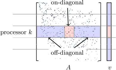
Fig. 3: Matrix $A$ and vector $v$ distributed across processes in a row-wise partition.

2.1 Method of non-Galerkin coarse-grids

In this section we give an overview of the method [11] which constructs hierarchies with coarse operators that do not satisfy the Galerkin relationship where $A_{\ell+1}=P_{\ell}^{T}A_{\ell}P_{\ell}$ for each level $\ell$. The method of non-Galerkin coarse-grids forms the coarse-grid operator through the Galerkin product, but then uses a sparsification step that generates $\vphantom{A}\smash[t]{\hat{A}}_{\ell+1}$ — see the call to sparsify in Algorithm 1. As motivated in the previous section, fewer nonzeros in the coarse-grid operator reduce the communication requirements. The sparser matrix $\vphantom{A}\smash[t]{\hat{A}}_{\ell+1}$ replaces $A_{\ell+1}$ and is then used when forming the remaining levels of the hierarchy, creating a dependency between $\vphantom{A}\smash[t]{\hat{A}}_{\ell+1}$ and all successive levels as shown in Figures 6(a) and 6(b). Thus, this approach does not preserve a coarse-grid correction corresponding to an $A$-orthogonal projection, as described in Section 2.

In the following we use edges$(A)$, for a sparse matrix $A$, to represent the set of edges in the graph of $A$. That is, ${\textnormal{{edges}}}(A)=\{(i,j)\,\text{such that}\,A_{i,j}\neq 0\}$, where $A_{i,j}={\left(A\right)}_{i,j}$ is the ${(i,j)}^{\text{th}}$ entry of $A$. In addition, we denote $\vphantom{P}\smash[t]{\hat{P}}_{\ell}$ as the injection interpolation operator that injects from level $\ell+1$ to the $C$ points on level $\ell$ so that $\vphantom{P}\smash[t]{\hat{P}}_{\ell}$ is defined as the identity over the coarse points.

The sparsify method for reducing the nonzeros in a matrix is described in Algorithm 3. Here, the method selectively removes small entries outside a minimal sparsity pattern given by $\mathcal{M}_{\ell}$ where ${\textnormal{{edges}}}(\mathcal{M}_{\ell})={\textnormal{{edges}}}(\vphantom{P}\smash[t]{\hat{P}}_{\ell}^{T}A_{\ell}P_{\ell}+P_{\ell}^{T}A_{\ell}\vphantom{P}\smash[t]{\hat{P}}_{\ell})$. For notational convenience, we set $A$ to $A_{\ell}$ as well as other operators in the algorithm. For a given tolerance $\gamma$, any entry $A_{i,j}$ with $(i,j)\notin\mathcal{M}$ and $\left\lvert A_{i,j}\right\rvert<\gamma\max_{k\neq i}\left\lvert A_{i,k}\right\rvert$ is considered insignificant and is removed. When entry $A_{i,j}$ is removed, the value of $A_{i,j}$ is lumped to other entries that are strongly connected to $A_{i,j}$, and $A_{i,j}$ is set to zero. This reduces the per-iteration communication complexity and heuristically targets spectral equivalence between the sparsified operator and the Galerkin operator [11, 20].

There is a trade-off between the communication requirements and the convergence rate. Each entry in the matrix has a communication cost that is dependent on the number of network links that the corresponding message travels in addition to network contention. In addition, each entry in the matrix also influences convergence of AMG, with large entries generally having larger impact (although this is not uniformly the case). Any entry that has an associated communication cost outweighing the impact on convergence should be removed. However, while it is possible to predict this communication cost based on network topology and message size, the entry’s contribution to convergence cannot be easily predetermined. When dropping via non-Galerkin coarse-grids, if the chosen drop tolerance is too large, too many entries are removed and convergence deteriorates. Because the ideal drop tolerance is problem dependent and cannot be predetermined, it is likely that the chosen drop tolerance is suboptimal.

Input:

$A_{c}$	coarse-grid operator
$A$	fine-grid operator
$P$	interpolation
$\vphantom{P}\smash[t]{\hat{P}}$	injection
$S$	classical strength matrix
$\gamma$	sparse dropping threshold parameter

Output: $\vphantom{A}\smash[t]{\hat{A}}_{c}$, a sparsified $A_{c}$

$\vphantom{P}\smash[t]{\hat{P}}\leftarrow{\textnormal{{form-injection()}}}$

$\mathcal{M}={\textnormal{{edges}}}(\vphantom{P}\smash[t]{\hat{P}}^{T}AP+P^{T}A\vphantom{P}\smash[t]{\hat{P}})$

  {Edges in the minimal sparsity pattern}

$\mathcal{N}=\emptyset$

  {Edges to keep in $A_{c}$}

$\vphantom{A}\smash[t]{\hat{A}}_{c}={\bf 0}$

  {Initialize sparsified $A_{c}$}

for ${\left(A_{c}\right)}_{i,j}\neq 0$ do

       if $(i,j)\in\mathcal{M}$ or $\left\lvert{\left(A_{c}\right)}_{i,j}\right\rvert\geq\gamma\max_{k\neq i}\left\lvert{\left(A_{c}\right)}_{i,k}\right\rvert$

             $\mathcal{N}\leftarrow\mathcal{N}\cup\{(i,j),(j,i)\}$ {Add strong edges or the required pattern}

      

for ${\left(A_{c}\right)}_{i,j}\neq 0$ do

       if $(i,j)\in\mathcal{N}$

             ${\left(\vphantom{A}\smash[t]{\hat{A}}_{c}\right)}_{i,j}={\left(\vphantom{\vphantom{A}\smash[t]{\hat{A}}_{c}}A_{c}\right)}_{i,j}$

            

      else

             $\mathcal{W}=\{k\,|\,S_{j,k}\neq 0,(i,k)\in\mathcal{N}\}$

              {Find strong neighbors in the keep list}

             for $k\in\omega$ do

                   $\alpha=\frac{\left\lvert S_{j,k}\right\rvert}{\sum_{m\in\mathcal{W}}\left\lvert S_{j,m}\right\rvert}$

                    {Relative strength to $k$}

                   ${\left(\vphantom{A}\smash[t]{\hat{A}}_{c}\right)}_{i,k}\leftarrow{\left(\vphantom{A}\smash[t]{\hat{A}}_{c}\right)}_{i,k}+\alpha{\left(A_{c}\right)}_{i,j}$

                   ${\left(\vphantom{A}\smash[t]{\hat{A}}_{c}\right)}_{k,i}\leftarrow{\left(\vphantom{A}\smash[t]{\hat{A}}_{c}\right)}_{k,i}+\alpha{\left(A_{c}\right)}_{i,j}$

                   ${\left(\vphantom{A}\smash[t]{\hat{A}}_{c}\right)}_{k,k}\leftarrow{\left(\vphantom{A}\smash[t]{\hat{A}}_{c}\right)}_{k,k}-\alpha{\left(A_{c}\right)}_{i,j}$

                  

            

      

Algorithm 3 sparsify from [11]

for ${\left(A_{c}\right)}_{i,j}\neq 0$ do

      1 ${\textnormal{{ismax}}}\leftarrow\left\lvert{\left(A_{c}\right)}_{i,j}\right\rvert=\max_{k\neq i}\left\lvert{\left(A_{c}\right)}_{ik}\right\rvert\,{\textnormal{{and}}}\,(i,k)\notin\mathcal{N}\,\forall\,k\neq i\,{\textnormal{{and}}}\,\sum_{j}{A_{i,j}}=0$

       if $(i,j)\in\mathcal{N}$ or ismax {Keep if entry is the single, maximum nonzero}

            2 ${\left(\vphantom{A}\smash[t]{\hat{A}}_{c}\right)}_{i,j}={\left(A_{c}\right)}_{i,j}$

      else {Otherwise add to the diagonal}

            ${\left(\vphantom{A}\smash[t]{\hat{A}}_{c}\right)}_{i,i}\leftarrow{\left(\vphantom{A}\smash[t]{\hat{A}}_{c}\right)}_{i,i}+{\left(A_{c}\right)}_{i,j}$

            

      

Diagonal Lumping – Alternative for loop (§ 3.1)

Figures 4(a) and 4(b) show the convergence and communication complexity, respectively, of various AMG hierarchies for solving a 3D Poisson problem with the method of non-Galerkin coarse-grids. The original Galerkin hierarchy converges in the fewest number of iterations, but has the highest communication complexity. Non-Galerkin removes an ideal number of nonzeros from coarse-grid operators (labeled ideal) when no entries are removed from the first coarse level, and all successive levels have a drop tolerance of 1.0. In this case, the communication complexity of the solver is greatly reduced with little effect on convergence. However, if the first coarse level is also created with a drop tolerance of 1.0, essential entries are removed (labeled too many). While the complexity of the hierarchy is further reduced, but the method fails to converge.

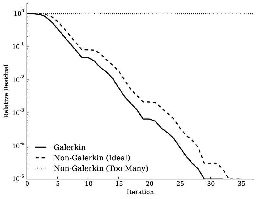
(a) Relative residual per iteration

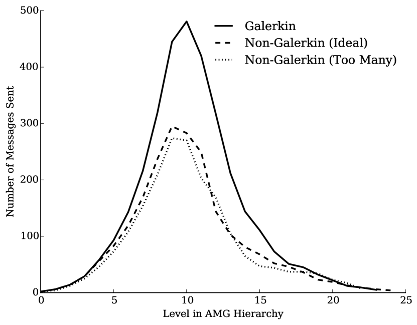
(b) Number of MPI sends per level

Fig. 4: Adding sparsity to AMG hierarchy

If a large drop tolerance is chosen for non-Galerkin AMG, the effect on convergence can be determined after one or two iterations of the solve phase. At this point, if convergence is poor, eliminated entries can be re-introduced into the matrix. However, with this method, convergence improvements cannot be guaranteed. As shown in Algorithm 1, sparsifying on a level affects all coarser-grid operators. Hence, adding entries back into the original operator does not influence the impact of their removal on all coarser levels. Figure 5 shows how re-adding entries is ineffective by plotting the required communication costs verses the achieved convergence for both Galerkin and non-Galerkin AMG solve phases for the same 3D Poisson problem. The data set Non-Galerkin (added back) is generated by removing entries with a drop tolerance of 1.0 (everything outside of $\mathcal{M}$) on the first coarse-grid operator and 0.0 (retaining everything) on all successive levels. This results in a non-convergent method. We then add these removed entries back into the first coarse-grid operator, but this does not reintroduce the entries which were removed from coarser grid operators as a result of the non-Galerkin triple-matrix product $P^{T}_{\ell}\vphantom{A_{\ell}}\smash[t]{\hat{A_{\ell}}}P_{\ell}$. Figure 5 shows that this hierarchy requires little coarse-level communication after all entries have been reinstated to the first coarse-grid operator. However as the required entries are not added back into all coarser grid operators, the method still fails to converge.

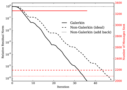
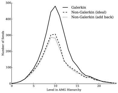
Fig. 5: Convergence vs. communication of Galerkin and non-Galerkin hierarchies for the Poisson problem. Relative residual per AMG iteration (black) vs the number of MPI sends per iteration (red) (left), and number of sends per level in AMG hierarchy (right)

3 Sparse and Hybrid Galerkin approaches

In this section we present two methods as alternatives to the method of non-Galerkin coarse-grids. The methods consist of forming the entire Galerkin hierarchy before sparsifying each operator, yielding a lossless approach for increasing sparsity in the AMG hierarchy. The first method, which is called the Sparse Galerkin method is described in Algorithm 4 (see Line 4). Sparse Galerkin creates the entire Galerkin hierarchy as usual. The hierarchy is then thinned as a post-processing step to remove relatively small entries outside of the minimal sparsity pattern $\mathcal{M}=\vphantom{P}\smash[t]{\hat{P}}^{T}AP+P^{T}A\vphantom{P}\smash[t]{\hat{P}}$ using sparsify.

Input:

$A_{0}$	fine-grid operator
max_size:	threshold for max size of coarsest problem
$\gamma_{1}$, $\gamma_{2}$, $\dots$	drop tolerances for each level
sparse_galerkin	Sparse Galerkin method
hybrid_galerkin	Hybrid Galerkin method

Output: $\vphantom{A}\smash[t]{\hat{A}}_{1},\dots,\vphantom{A}\smash[t]{\hat{A}}_{\ell_{\max}}$

$A_{1},\dots,A_{\ell_{\text{max}}},P_{0},\dots,P_{\ell_{\text{max}}-1}={\textnormal{{amg\_setup}}}(A_{0},{\textnormal{{max\_size}}},{\textnormal{{False}}})$

$\vphantom{A}\smash[t]{\hat{A}}_{0}=A_{0}$

for $\ell\leftarrow 1$ to $\ell_{\text{max}}$ do

       if sparse_galerkin

            1 $\vphantom{A}\smash[t]{\hat{A}}_{\ell+1}$ = sparsify($A_{\ell+1}$, $A_{\ell}$, $P_{\ell}$, $S_{\ell}$, $\gamma_{\ell}$)

              {Increase using the Sparse Method}

            

       else if hybrid_galerkin

            2 $\vphantom{A}\smash[t]{\hat{A}}_{\ell+1}$ = sparsify($A_{\ell+1}$, $\vphantom{A}\smash[t]{\hat{A}}_{\ell}$, $P_{\ell}$, $S_{\ell}$, $\gamma_{\ell}$)

              {Increase using the Hybrid Method}

            

      

Algorithm 4 sparse_hybrid_setup

The second method that we introduce is called Hybrid Galerkin since it combines elements of Galerkin and Sparse Galerkin to create the final hierarchy. The method is again lossless, and is outlined in Algorithm 4 (see Line 4). After the Galerkin hierarchy is formed, small entries outside are removed, this time using a modified, minimal sparsity pattern of $\mathcal{M}=\vphantom{P}\smash[t]{\hat{P}}^{T}\vphantom{A}\smash[t]{\hat{A}}P+P^{T}\vphantom{A}\smash[t]{\hat{A}}\vphantom{P}\smash[t]{\hat{P}}$.

The Sparse and Hybrid Galerkin methods retain the structure of the original Galerkin hierarchy. Consequently, these methods introduce error only into relaxation and residual calculations. The remaining components of each V-cycle in the solve phase (see amg_solve), such as restriction and interpolation are left unmodified. Therefore, the grid transfer operators do not depend on any sparsification, as shown in Figure 6. Here, we see that the Sparse Galerkin method does not use the modified (or sparsified) operators to create the next coarse-grid operator in the hierarchy. Conversely, Hybrid Galerkin uses the newly modified operator to compute the sparsity pattern $\mathcal{M}$ for the next coarse-grid operator; this process does not impact interpolation.

(a) Galerkin

(b) Non-Galerkin

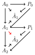
(c) Sparse Galerkin

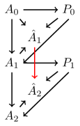
(d) Hybrid Galerkin

Fig. 6: Dependencies for forming each operator in the various AMG hierarchies. The difference between Sparse and Hybrid Galerkin dependencies is highlighted in red.

The new Sparse Galerkin and Hybrid Galerkin methods reduce the per-iteration cost in the AMG solve cycle as less communication is required by each sparse, coarse-grid operator. However, high-energy error may also be relaxed at a slower rate, yielding a reduction in the convergence factor. As a result, the solve phase is more efficient when the reduction in communication outweighs the change in convergence factor.

Similar to the method of non-Galerkin, it is difficult to predict the impact of removing entries from $A_{c}$ on the relaxation process. However, as the structure of the Galerkin hierarchy is retained, the convergence factor of the solve phase can be controlled on-the-fly. In our approach, differences between $A_{c}$ and $\vphantom{A_{c}}\smash[t]{\hat{A_{c}}}$ are stored while forming the sparse approximations. Subsequently, if the convergence factor falls below a tolerance, entries can be reintroduced into the hierarchy, allowing improvement of the convergence factor up to that of the original Galerkin hierarchy (see Section 6).

3.1 Diagonal Lumping

A significant amount of work is required in Algorithm 3 to increase the sparsity of each coarse operator. When forming non-Galerkin coarse-grids, this additional setup cost is hidden by the reduced cost of the sparsified triple matrix product $A_{c}=P^{T}\vphantom{A}\smash[t]{\hat{A}}P$. However, as the entire Galerkin hierarchy is initially formed as usual in our new methods (Algorithm 4) the additional work greatly reduces the scalability of the setup phase, as shown in Section 5.2. This significant cost suggests using an alternative method for sparsification of coarse-grid operators. When reducing the number of nonzeros from coarse-grid operators with Sparse Galerkin or with Hybrid Galerkin, the structure of the Galerkin hierarchy remains intact, allowing a more flexible treatment of increasing sparsity in the matrix. For instance, one option is to remove entries by lumping to the diagonal rather than strong neighbors, as described in Algorithm 3b. This variation of sparsify is beneficial for several reasons, including a much cheaper setup phase when compared to Algorithm 3, potential to reduce the cost of the solve phase, reduced storage constraints for adaptive solve phases (see Algorithm 5), and retaining positive-definiteness of coarse operators.

Algorithm 3b replaces the for loop in Algorithm 3. For each nonzero entry in the matrix, the algorithm first checks if the entry is the maximum element in the row and if all other entries in the row are selected for removal (see Line 2.1). In this case, the nonzero entry is not removed if there is a zero row sum.

The method of diagonal lumping (Algorithm 3b) results in a significantly cheaper setup phase than Algorithm 3. The original non-Galerkin sparsify requires each removed entry to be symmetrically lumped to significant neighbors. As a result, the process of calculating the associated strong connections requires a large amount of computation. Furthermore, to maintain symmetry, all matrix entries that are not stored locally must be updated, requiring a significant amount of interprocessor communication. Lumping these entries to the diagonal eliminates both the computational and communication complexities.

Eliminating the requirement of lumping to strong neighbors yields potential for removing a larger number of entries from the hierarchy, further reducing the communication costs of the solve phase. The original version of Algorithm 3 requires that an entry must have strong neighbors to be removed, as its value is lumped to these neighbors.

While relaxing the restrictions of the original non-Galerkin sparsify provides more opportunity to remove entries from the matrix, the diagonal lumping also negatively influences convergence in some cases. However, during the solve phase, if convergence suffers, entries can be easily reintroduced into the hierarchy, improving convergence. As removed entries are only added to the diagonal, the storage of both the sparse matrix along with removed entries is minimal. In addition, these entries can be restored simply by adding their values to the original positions, and subtracting these values from the associated diagonal entries as shown in Algorithm 5. The process of reintroducing these entries requires no interprocessor communication as well as a low amount of local computational work.

Diagonal lumping also preserves matrix properties such as symmetric positive-definiteness (SPD). As described in the following theorem, if the sparsity of a diagonally dominant, SPD matrix is increased using diagonal lumping, the resulting matrix remains SPD. Consequently, Sparse and Hybrid Galerkin with diagonal lumping can be used in preconditioning many methods such as conjugate gradient. It is important to note, that while SPD matrices are an attractive property for AMG, AMG methods do not guarantee diagonally dominance of the coarse-grid operators. Yet, in many instances this property is preserved, for example for more standard elliptic operators.

Theorem 1.

Let $A$ be SPD and diagonally dominant. If $\vphantom{A}\smash[t]{\hat{A}}$ is produced by Algorithm 3b, then it is symmetric positive semi-definite and diagonally dominant.

Proof.

Let $A$ be SPD with diagonal dominance,

(2) $$\left|A_{i,i}\right|\geq\sum_{k\neq i}\left|A_{i,k}\right|,\forall i.$$

Symmetry of $\vphantom{A}\smash[t]{\hat{A}}$ is guaranteed from the symmetry of both $A$ and the $\mathcal{N}$ from Algorithm 3. For all off-diagonal entries $(i,j),(j,i)\in\mathcal{N}$,

(3) $$\vphantom{A}\smash[t]{\hat{A}}_{i,j}=A_{i,j}=A_{j,i}=\vphantom{A}\smash[t]{\hat{A}}_{j,i},$$

by Line 2.1 in Algorithm 3b and the symmetry of $A$.

The positive-definiteness is guaranteed by the diagonal dominance and a Gershgorin disc argument. The proof proceeds by starting with the matrix $A$ and then considering the change made to $A$ by the elimination of each entry. Initially, all the Gershgorin discs of $A$ are strictly on the right-side of the origin, thus implying that all eigenvalues are non-negative. Then, assume that we eliminate some arbitrary entry $A_{i,j}$, $(i,j)\in\mathcal{N}$. This results in row $i$ being updated

(4) $$A_{i,i}\leftarrow A_{i,i}+A_{i,j}\quad\mbox{and}\quad A_{i,j}\leftarrow 0$$

If $A_{i,j}>0$, then the center of the Gershgorin disc is shifted to the right, and the radius shrinks, thus keeping the disc to the right of the origin and preserving definiteness. If $A_{i,j}<0$, then the center of the disc is shifted to the left by $|A_{i,j}|$, but the radius of the disc also shrinks by $|A_{i,j}|$. This also keeps the disc to the right of the origin and preserves semi-definiteness. Furthermore, since each disc is never shifted to the left, diagonal dominance is also preserved. The proof then proceeds by considering all of the entries to be eliminated. ∎

Remark 3.1.

If any row of $A$ is strictly diagonally dominant, as often happens with Dirichlet boundary conditions, then $\vphantom{A}\smash[t]{\hat{A}}$ will be positive definite. Essentially, Algorithm 3b never shifts a Gershgorin disc to the left, so $\vphantom{A}\smash[t]{\hat{A}}$ can have no $0$ eigenvalue.

4 Parallel Performance

In this section we model the parallel performance of Galerkin, non-Galerkin, Sparse and Hybrid Galerkin using full lumping as in Algorithm 3, and Sparse and Hybrid Galerkin with diagonal lumping as in Algorithm 3b (labeled with Diag) in order to illustrate the per-level costs associated with each method. The large increase in cost on coarse-levels in the Galerkin method (see Figure 2) is due to the increase in coarse-level communication.

The solve phase of AMG (see Algorithm 2) is largely comprised of sparse matrix-vector multiplication, thus we model each method by assessing the cost of performing a SpMV on each level of the hierarchy. We focus on the operators $A_{\ell}$, as the work required for this matrix is more costly than the restriction and interpolation operations. Specifically, we employ an $\alpha$–$\beta$ model to capture the cost of the parallel SpMV based on the number of nonzeros in $A$. We denote $p$ as the number of processors, $\alpha$ as the latency or startup cost of a message, and $\beta$ as the reciprocal of the network bandwidth [12, 13]. In addition, $\textnormal{{nnz}}_{p}$ represents the average number of nonzeros local to a process, while $s_{p}$ and $n_{p}$ are the maximum number of MPI sends and message size across all processors. Finally, we use $c$ to represent the cost of a single floating-point operation. With this we model the total time as

(5) $$T=2\,c\,\textnormal{{nnz}}_{p}+\max_{p}s_{p}(\alpha+\beta n_{p}).$$

For the model parameters above we us the Blue Waters supercomputer at the University of Illinois at Urbana-Champaign [1, 4]. The latency and bandwidth were measured through the HPCC benchmark [15], yielding $\alpha=$1.8\text{\times}{10}^{-6}$$ and $\beta=$1.8\text{\times}{10}^{-9}$$. Since the achieved floprate depends on matrix size, we determine the value of $c$ by timing the local SpMV. Specifically, letting $\textnormal{{nnz}}_{\text{local}}$ be the number of nonzeros local to the processor and $T_{\text{local}}$ the time to perform the local portion of the SpMV, we compute $c=\nicefrac{{T_{\text{local}}}}{{2\textnormal{{nnz}}_{\text{local}}}}$ for each matrix in the hierarchy.

The minimal per-level cost associated with the non-Galerkin and Sparse/Hybrid Galerkin methods occurs when entries are removed with a drop tolerance of $\gamma=1.0$. Using the model, (5), this is highlighted in Figure 7 for both the Laplace and rotated anisotropic diffusion problems (a full description of these problems is given in Section 5. We see that both non-Galerkin and Hybrid Galerkin have potential to minimize the per-level cost. However, when the per-level cost is minimized, the convergence of AMG often suffers. Therefore, less-aggressive drop tolerances such as $\gamma<1.0$ may remove fewer entries, increasing the per-level cost, but due to better convergence will improve the overall cost of the solve phase.

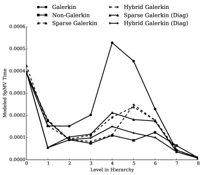
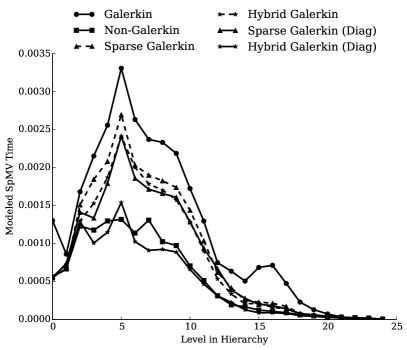
Fig. 7: Modeled minimal cost of a single SpMV on each level of the AMG hierarchy for Laplace (left) and rotated anisotropic diffusion (right), for an aggressive drop tolerance of 1.0 on each level.

Figure 8 models the cost of a SpMV on each level of the hierarchy in the case of more realistic drop tolerances that are used to retain convergence of the original method. These drop tolerances vary by level in the AMG hierarchy, each containing a combination of $0.0$, $0.01$, $0.1$, and $1.0$. For each test displayed in the model, six drop tolerance series were tested, and we selected the smallest solve time. The results underscore the simplicity of the Laplacian, as removing entries can fortuitously improve convergence of this problem. For the rotated anisotropic diffusion problem the per-level cost of non-Galerkin and Hybrid Galerkin increase in order to retain convergence. However, the per-level cost of the non-Galerkin and Hybrid/Sparse Galerkin methods are significantly decreased for levels near the middle of the hierarchy.

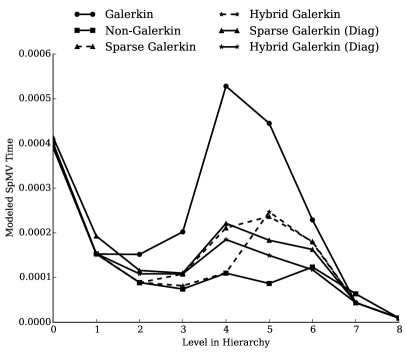
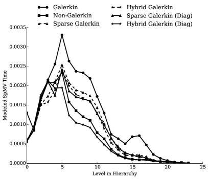
Fig. 8: Modeled minimal cost of a single SpMV on each level of the AMG hierarchy for Laplace (left) and rotated anisotropic diffusion (right) when a practical drop tolerance is used.

5 Parallel results for Sparse and Hybrid Galerkin

In this section we highlight the parallel performance of the Sparse and Hybrid Galerkin methods. We consider scaling tests on the familiar 3D Laplacian since this is a common multigrid problem used to establish a baseline. In order to test problems where AMG convergence is suboptimal, we consider the 2D rotated anisotropic diffusion problem. Finally, we test our methods on a suite of matrices from the Florida Sparse Matrix Collection. All computations were performed on the Blue Waters system at the University of Illinois at Urbana-Champaign [1]. Each method was implemented and solved with hypre [2, 14], using default parameters unless otherwise specified. In summary, we compare the solve and setup times of the four methods discussed in previous sections, preconditioning a Krylov method such as CG or GMRES in each test:

Galerkin:

Classic coarsening in AMG, as outlined in Algorithm 1;

non-Galerkin

The base algorithm presented in [11], where $P^{T}AP$ is not used on coarse-levels;

Sparse Galerkin

A new algorithm presented in Algorithm 4; and

Hybrid Galerkin

A new algorithm presented in Algorithm 4.

In addition, we also consider the Sparse and Hybrid Galerkin methods with diagonal lumping, as detailed in Algorithm 3b. The drop tolerances for each method vary by level, using a combination of $0.0$, $0.01$, $0.1$, and $1.0$ across the coarse-levels. Six combinations of these drop tolerances are tested for the various test cases, and the series yielding the minimum solve time for each is selected. note: At $100,000$ cores, the best drop tolerances from the second largest run size are used due to large costs associated with running 6 drop tolerances at this core count.

We consider the diffusion problem

(6) $$-\nabla\cdot K\nabla u=0,$$

with two particular test cases for our simulations:

3D Laplacian

Here, we use $K=I$ on the unit cube with homogeneous Dirichlet boundary conditions. Q1 finite elements are used to discretize the problem using a uniform mesh, leading to a familiar 27-point stencil. The preconditioner formed for the 3D Laplacian uses aggressive coarsening (HMIS) and distance-two (extended classical modified) interpolation. The interpolation operators were formed with a maximum of five elements per row, and hybrid symmetric Gauss-Seidel was the relaxation method.

Rotated, anisotropic diffusion

In this case, we consider a diffusion tensor with homogeneous Dirichlet boundary conditions of the form $K=Q^{T}DQ$, where $Q$ is a rotation matrix and $D$ is a diagonal scaling defined as

(7) $$Q=\left(\begin{matrix}\cos(\theta)&\sin(\theta)\\ -\sin(\theta)&\cos(\theta)\end{matrix}\right)\qquad D=\left(\begin{matrix}1&0\\ 0&\epsilon\end{matrix}\right).$$

Q1 finite elements are used to discretize a uniform, square mesh. In the following tests we use $\theta=\frac{\pi}{8}$ and $\epsilon=0.001$. In each case, the preconditioner uses Falgout coarsening [7], extended classical modified interpolation and hybrid symmetric Gauss-Seidel.

Lastly, as problems with less structure result in increased density on coarse-levels, we consider a subset from the Florida sparse matrix collection.

Florida sparse matrix collection subset

We consider all real, symmetric, positive definite matrices from the Florida sparse matrix collection with size over 1,000,000 degrees-of-freedom. In addition we consider only the cases where GMRES preconditioned with Galerkin AMG converges in fewer than 100 iterations. Each problem uses HMIS coarsening and so-called extended+i interpolation if possible. In some cases, however, Galerkin AMG does not converge with these options; in these cases Falgout coarsening and modified classical interpolation are used. Relaxation for all systems is hybrid symmetric Gauss-Seidel. note: When necessary for convergence, some hypre parameters, such as the minimum coarse-grid size and strength tolerance, vary from the default.

The following results demonstrate that the diagonally lumped Sparse and Hybrid Galerkin methods are able to perform comparably to non-Galerkin. Non-Galerkin and Sparse/Hybrid Galerkin all significantly reduce the per-iteration cost by reducing communication on coarse-levels. Since the method of non-Galerkin is multiplicative in construction, the setup times are often much lower in comparison to standard Galerkin. However, Sparse and Hybrid do not observe this benefit since the processing is post facto. While the per-iteration work is decreased for all methods, the convergence suffers for the case of rotated anisotropic diffusion problems with non-Galerkin at large scales. However, Sparse and Hybrid Galerkin converge at rates similar to the original Galerkin hierarchy, yielding speedup in total solve times.

A strong scaling study shows that the anisotropic problem of a set size can be most efficiently solved at larger scales when using non-Galerkin, but Hybrid Galerkin performs comparably. Lastly, a strong scaling study of the subset of Florida sparse matrix collection problems shows that non-Galerkin and Sparse/Hybrid Galerkin each improve solve phase times for all matrices. While non-Galerkin performs slightly better for many problems on $32$ cores, Hybrid Galerkin outperforms the other methods for most problems at larger scales.

5.1 Increasing sparsity in AMG Hierarchies

The significant number of nonzeros on coarse-levels creates large, relatively dense matrices near the middle of the AMG hierarchy, yielding large communication costs for each SpMV performed on these levels. As the solve phase of AMG consists of many SpMVs on each level of the hierarchy, the time spent on coarse-levels can increase dramatically. Sparse, Hybrid, and non-Galerkin can all reduce both the cost associated with communication as well as the time spent on each level during a solve phase.

Figure 9 shows the time spent on each level of the hierarchy during a single iteration of AMG, for both test cases with 10,000 degrees-of-freedom per core using 8192 cores. Both the method of non-Galerkin coarse-grids, as well as the Sparse and Hybrid Galerkin methods, reduce the time required on levels near the middle of the hierarchy. Non-Galerkin more greatly reduces the time spent on middle levels of the hierarchy for the Laplace problem than Sparse and Hybrid Galerkin. However, for the anisotropic problem, diagonally-lumped Hybrid Galerkin reduces level-time equivalently. This is due to a large reduction in the number of messages required in each SpMV as shown in Figure 10. The reduction in total size of all messages communicated is relatively small.

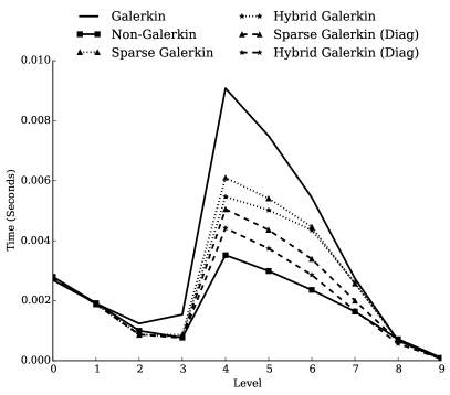
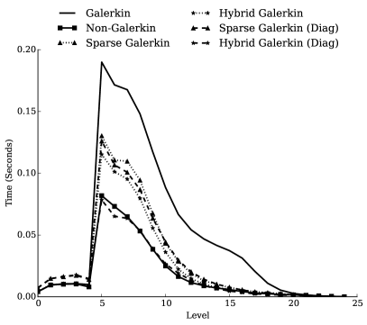
Fig. 9: Time spent on each level of the AMG hierarchy during a single iteration of the solve phase for Laplace (left) and rotated anisotropic diffusion (right), each with 10,000 degrees-of-freedom per core.

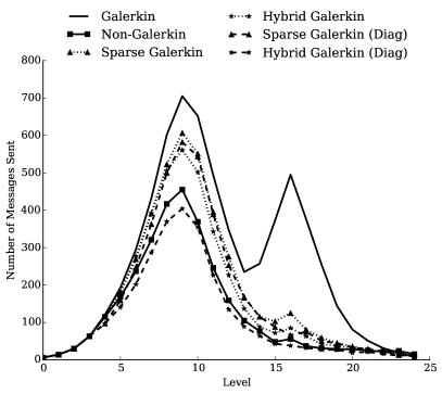
Fig. 10: Number of sends required to perform a single SpMV on each level of the AMG hierarchy for: Laplace (left) and Rotated anisotropic diffusion (right), each with 10,000 degrees-of-freedom per core.

The increase in time spent on each level, as well as the associated communication costs of these levels, becomes more pronounced at higher processor counts in a strong scaling study. Figure 11 illustrates this by plotting the per-level times required during a single iteration of AMG, as well as the number of messages communicated during a SpMV for the rotated anisotropic diffusion problem with 1,250 degrees-of-freedom per core using 8192 cores. Compared with the 10,000 degrees-of-freedom per core example in Figures 10 and 9, there is a sharper increase in time required for levels near the middle of the hierarchy due to the increasing dominance of communication complexity. note: Strong scaling the Laplace problem results in similar performance.

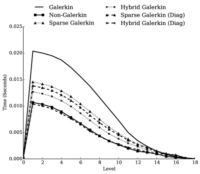
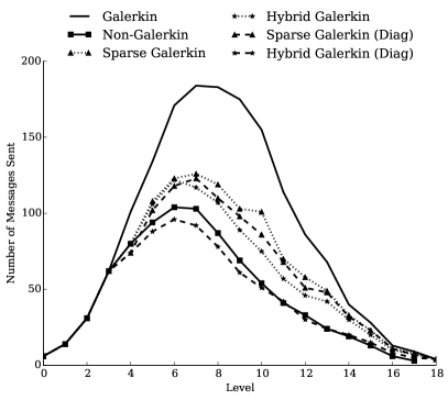
Fig. 11: For each level of the AMG hierarchy, time per iteration of AMG (left) and number of messages sent during a single SpMV (right) for the rotated anisotropic diffusion problem with 1,250 degrees-of-freedom per core.

5.2 Costs of Weakly Scaled Setup Phases

Each sparsification method can lead to reduced communication costs in the middle of the hierarchy. However, removing insignificant entries from coarse-grid operators requires additional work in the setup phase. In the non-Galerkin method, setup times are reduced since the increased sparsity is used directly in the triple-matrix product required to form each successive coarse-grid operator. However, for the new methods, Sparse and Hybrid Galerkin, the entire Galerkin hierarchy is first constructed so that the sparsify process on each level requires additional work. Figure 12 shows the times required to setup an AMG hierarchy for rotated anisotropic diffusion, with Laplace setup times scaling in a similar manner. While there is a slight increase in setup cost associated with the Sparse and Hybrid Galerkin hierarchies, this extra work is nominal. Therefore, while the majority of this additional work is removed when using diagonal lumping, the differences in work required in the setup phase between these two lumping strategies is insignificant for the problems being tested.

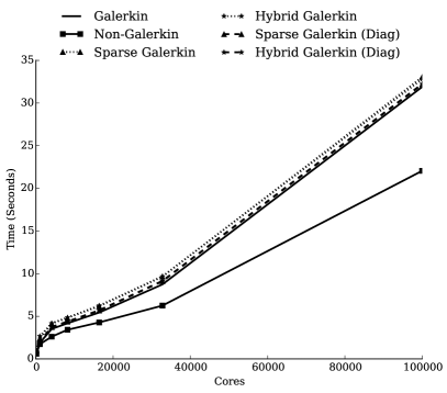
Fig. 12: Time required to setup AMG hierarchy for rotated anisotropic diffusion with 10,000 degrees-of-freedom per core.

5.3 Weak Scaling of GMRES Preconditioned by AMG

In this section we investigate the weak scaling properties of the methods. Figure 13 shows both the average convergence factor and total time spent in the solve phase for a weak scaling study with rotated anisotropic diffusion problems at 10,000 degrees-of-freedom per core using GMRES preconditioned by AMG. GMRES is used over CG because Algorithm 3 guarantees symmetry but not positive-definiteness of the preconditioner. In many cases, positive-definiteness is preserved, but when using more aggressive drop tolerances, we have observed this property being lost. While the convergence of both diagonally-lumped Sparse and Hybrid Galerkin remain similar to that of Galerkin, the non-Galerkin method converges more slowly. Therefore, while non-Galerkin and diagonally-lumped Hybrid Galerkin yield similar communication requirements, GMRES preconditioned by Hybrid Galerkin performs significantly better as fewer iterations are required.

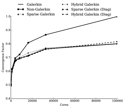
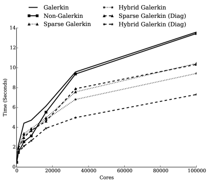
Fig. 13: Convergence factors (left) and times (right) for weak scaling of anisotropic problem (10,000 degrees-of-freedom per core), solved by preconditioned GMRES. For large problem sizes, non-Galerkin AMG does not converge, and timings indicate when the maximum iteration count was reached.

Remark 5.1.

With the chosen drop tolerances, non-Galerkin does not converge for this anisotropic problem at $100,000$ cores. In this case, nothing was dropped from the first three coarse-levels of the hierarchy. On the fourth coarse-level a drop tolerance of $0.01$ was used, and the fifth was sparsified with a tolerance of $0.1$. The remaining levels were sparsified with a drop tolerance of $1.0$. This was determined to be the best tested drop tolerance sequence for smaller run sizes, and multiple drop tolerance sequences were not tuned at this large problem size due to the significant costs. However, a better drop tolerance could yield a convergent non-Galerkin method at this scale.

The efficiency of weakly scaling to $p$ processes is defined as $E_{p}=\frac{T_{p}}{pT_{1}}$, where $T_{1}$ is the time required to solve the problem on a single process and $T_{p}$ is time to solve on $p$ processes. The efficiency of solving weakly scaled rotated anisotropic diffusion problems with non-Galerkin, Sparse Galerkin, and Hybrid Galerkin, relative to the efficiency of Galerkin AMG, are shown in Figure 14. While both the original and diagonally-lumped Sparse and Hybrid Galerkin methods scale more efficiently than Galerkin, the poor convergence of non-Galerkin on large run sizes yields a reduction in relative efficiency. While the methods perform similarly when solving the Laplace problem, non-Galerkin improves relative efficiency for all scalings of this model problem.

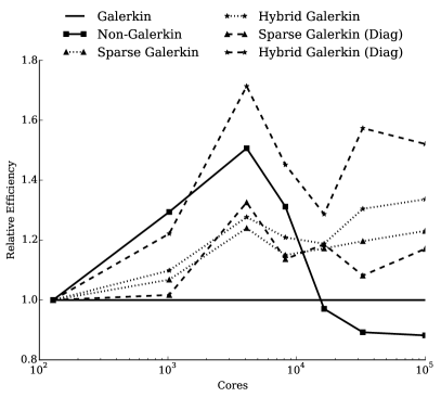
Fig. 14: Efficiency of solving weakly scaled rotated anisotropic diffusion at 10,000 degrees-of-freedom per core with various methods, relative to that of the Galerkin hierarchy.

5.4 Strong Scaling of GMRES Preconditioned by AMG

We next consider the rotated anisotropic diffusion system with approximately $10,240,000$ unknowns using cores ranging from $128$ to $100,000$. Therefore, the simulation is reduced from $80,000$ degrees-of-freedom per core when run on $128$ cores, to just over $100$ degrees-of-freedom per core on $100,000$ cores. Computation dominates the total cost of solving a problem partitioned over relatively few processes, as each process has a large amount of local work. However, as the problem is distributed across an increasing number of processes, the local work decreases while communication requirements increase. Therefore, the time required to solve a problem is reduced with strong scaling, but only to the point where communication complexity begins to dominate. The efficiency of solving this problem with preconditioned GMRES relative to Galerkin is shown in Figure 15. In each case we observe improvements over standard Galerkin.

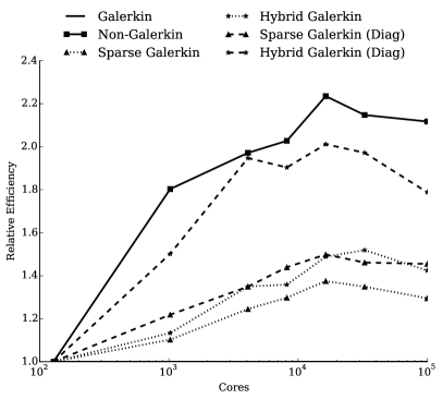
Fig. 15: Efficiency of non-Galerkin and Sparse/Hybrid Galerkin methods in a strong scaling study, relative to Galerkin AMG for rotated anisotropic diffusion.

A strong scaling study is also performed on the subset of matrices from the Florida sparse matrix collection. These problems were tested on $64$, $128$, $256$, and $512$ processes. Figure 16 shows the time required to perform a single V-cycle for each of the matrices in the subset, relative to the time required by Galerkin AMG. All methods reduce the per-iteration times for each matrix in the subset. Furthermore, the total time required to solve each of these matrices is also reduced, as shown in Figure 17. While Sparse Galerkin provides some improvement, the Hybrid and non-Galerkin methods are comparable, particularly at high core counts.

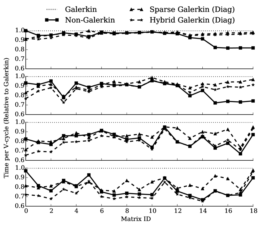
Fig. 16: Time (relative to Galerkin) per iteration for each matrix in the Florida Sparse Matrix Collection, using $p=64$, $128$, $256$, and $512$.

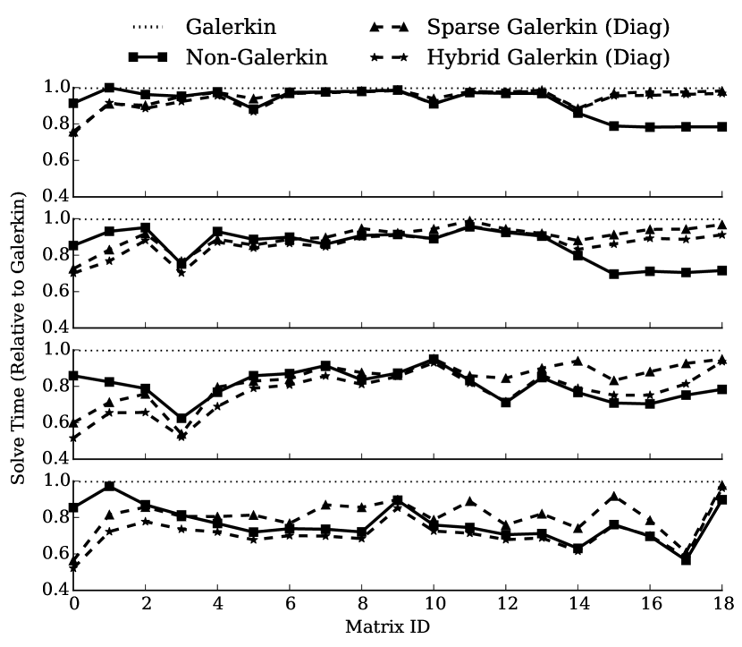
Fig. 17: Time (relative to Galerkin) per AMG solve for each matrix in the Florida Sparse Matrix Collection, using $p=64$, $128$, $256$, and $512$.

5.5 Diagonal Lumping Alternative and Preconditioned Conjugate Gradient

Diagonal lumping retains positive-definiteness of diagonally-dominant coarse-grid operators, as described in Theorem 1. Therefore, as the preconditioned Conjugate Gradient (PCG) method requires both the matrix and preconditioner to be symmetric and positive-definite, the Laplace and anisotropic diffusion problems are solved by Conjugate Gradient preconditioned by the diagonally-lumped Sparse and Hybrid Galerkin hierarchies. Figure 18 shows the solve phase times for solving the weakly scaled rotated anisotropic diffusion problem with PCG. As with GMRES, both the Sparse and Hybrid Galerkin preconditioners decrease the time required in the AMG solve phase during a weak scaling study.

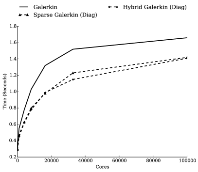
Fig. 18: Weak scaling solve time for the anisotropic problem, solved by PCG preconditioned by various AMG hierarchies.

6 Adaptive Solve Phase

The previous results describe the case of an optimal drop tolerance selected in sparsify: the new diagonally-lumped Sparse and Hybrid Galerkin methods reduce the cost of the solve phase. However, as the optimal drop tolerance changes with problem type, problem size, and even level of the AMG hierarchy, an optimal drop tolerance is often not easily realized. When the drop tolerance is too small, few entries are removed from the hierarchy and the communication complexity remains the same. However, if the drop tolerance is too large, the solver is non-convergent, as described in Section 2.1.

In this section we consider an adaptive method that attempts to add entries back into the hierarchy as a deterioration in convergence is observed. This is detailed in Algorithm 5. The algorithm initializes a Sparse or Hybrid Galerkin hierarchy and proceeds by executing $k$ iterations of a preconditioned Krylov method — e.g. PCG. If the convergence is below a tolerance, the coarse levels are traversed until a coarse grid operator is found on which entries were removed with a drop tolerance greater than $0.0$. Entries are then added back to this coarse-grid operator, reducing the drop tolerance by a factor of 10. Any new drop tolerance below $\gamma_{\text{min}}=0.01$ is rounded down to $0.0$. This continues until entries have been reintroduced into $s$ coarse-grid operators. At this point, the Krylov method continues, using the most recent values for $x$ unless the previous iterations diverged from the true solution. Many methods such as PCG and GMRES must be restarted after the preconditioner has been edited. This entire process is then repeated until convergence. The adaptive solve phase requires additional iterations over Galerkin AMG, as initial iterations of this method may not converge. However, the goal of this solver is to guarantee convergence similar to Galerkin AMG. Speed-up over Galerkin AMG is still dependent on choosing reasonable initial drop tolerances.

Input:

$A$, $b$, $x_{0}$
$\vphantom{A}\smash[t]{\hat{A}}_{1},\dots,\vphantom{A}\smash[t]{\hat{A}}_{\ell_{\max}}$	Sparse/Hybrid Galerkin coarse grid matrices
$A_{1},\dots,A_{\ell_{\max}}$	original Galerkin coarse grid matrices
$P_{0},\dots,P_{\ell_{\max}-1}$
$k$	number of PCG iterations before convergence test
$s$	number of AMG levels to update at a time
$\gamma_{0}$, $\gamma_{1}$, $\dots$	drop tolerance used at each level for sparsification
tol	convergence tolerance
sparse_galerkin	Sparse Galerkin method
hybrid_galerkin	Hybrid Galerkin method

Output: $x$

$x=x_{0}$

$r_{0}=b-Ax_{0}$

while $\nicefrac{{\|r\|}}{{\|r_{0}\|}}\leq{\textnormal{{tol}}}$

       $M={\textnormal{{preconditioner}}}({\textnormal{{amg\_solve}}},\vphantom{A}\smash[t]{\hat{A}}_{1},\dots,\vphantom{A}\smash[t]{\hat{A}}_{\ell_{\max}},P_{0},\dots,P_{\ell_{\max}-1})$

       $x=\text{PCG}(A,b,x,k,M)$

        {Call $k$ steps of preconditioned CG}

       $r=b-Ax$

       if $\frac{\|r\|}{\|r_{0}\|}\leq{\textnormal{{tol}}}$

             continue

            

       else

             for $\ell=0,\dots,\ell_{\text{max}}$ do

                   if $\gamma_{0}>0$

                         $\ell_{\text{start}}\leftarrow\ell$

                          {Find finest level that uses dropping}

                        

                  

             for $\ell=\ell_{\text{start}}\ldots\ell_{\text{start}}+s$ do

                   $\gamma_{\ell}=\begin{cases}\frac{\gamma_{\ell}}{10},&\text{if}\ \frac{\gamma_{\ell}}{10}>\gamma_{\text{min}}\\ 0,&\text{{{{otherwise}}}}\end{cases}$

                    {Determine new dropping parameter}

                   if sparse_galerkin {Re-add entries at the new dropping tolerance}

                         $\vphantom{A}\smash[t]{\hat{A}}_{\ell}=$sparsify$(A_{\ell}$, $A_{\ell-1}$, $P_{\ell-1}$, $S_{\ell-1}$, $\gamma_{\ell})$

                   else if hybrid_galerkin {Re-add entries at the new dropping tolerance}

                         $\vphantom{A}\smash[t]{\hat{A}}_{\ell}=$sparsify$(A_{\ell}$, $\hat{A}_{\ell-1}$, $P_{\ell-1}$, $S_{\ell-1}$, $\gamma_{\ell})$

                  

            

      

Algorithm 5 adaptive_solve

Example 6.1.

As an example, consider the case of a hierarchy with 6 levels using drop tolerances of $[0,0.01,0.1,1.0,1.0,1.0]$ — i.e., $\vphantom{A}\smash[t]{\hat{A}}_{1}$ retains all entries from $A_{1}$, $\vphantom{A}\smash[t]{\hat{A}}_{2}$ and $\vphantom{A}\smash[t]{\hat{A}}_{3}$ result from sparsify with $\gamma=0.01$ and $\gamma=0.1$, etc. Suppose that adaptive_solve with $k=3$ and $s=2$ results in 3 iterations of PCG and a large residual. The adaptive solve find the first level containing a sparsified coarse grid matrix, namely $\vphantom{A}\smash[t]{\hat{A}}_{2}$. The drop tolerance on this level is changed from $0.01$ to $0.0$, and the original coarse matrix $A_{2}$ is sparsified with to the new drop tolerance. Furthermore, since $s=2$ the drop tolerance on level $3$ is reduced from $0.1$ to $0.01$, and $A_{3}$ is also sparsified. PCG then restarts with the new hierarchy. If convergence continues to suffer after 3 iterations, the hierarchy is updated again, but since $\vphantom{A}\smash[t]{\hat{A}}_{2}$ has $\gamma_{2}=0.0$, entries are reintroduced into coarse matrices $\vphantom{A}\smash[t]{\hat{A}}_{3}$ and $\vphantom{A}\smash[t]{\hat{A}}_{4}$ instead.

Using Algorithm 5, Figure 19 shows both the relative residual of the system after each iteration as well as the communication costs of PCG using three different AMG hierarchies: standard Galerkin, Sparse Galerkin with diagonal lumping and aggressive dropping, and Sparse Galerkin with diagonal lumping modified with adaptivity. For the adaptive case, we purposefully choose an overly aggressive initial drop tolerance so that entries can be added back multiple times and one coarse level at a time to show the effect on convergence and communication. Initially, when the drop tolerance is aggressive, the associated communication costs are low, but the resulting PCG iterations do not converge; this provides a baseline. As sparse entries are reintroduced into the hierarchy, convergence improves, while only slightly increasing the associated communication cost. When entries are reintroduced into the hierarchy, the preconditioner for PCG changes, and hence, the method must be restarted. After restarting the method, convergence improves.

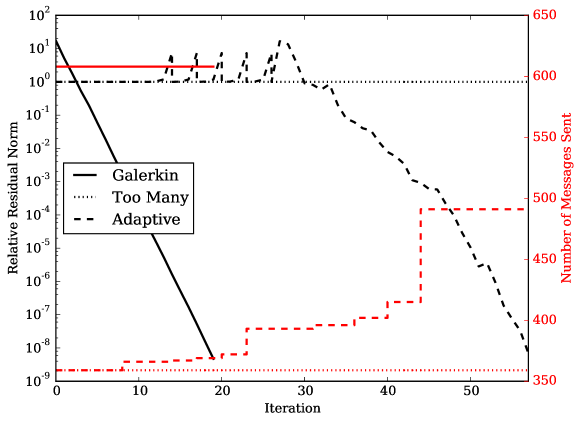
Fig. 19: Relative residual (black) and number of MPI sends (red) per iteration when solving the Laplace problem with: (1) PCG using Galerkin AMG; (2) Hybrid Galerkin with aggressive dropping (labeled Too Many); (3) Hybrid Galerkin solved with Algorithm 5, using $k=3$, $s=1$, and $\gamma_{l}\dots\gamma_{l_{\max}}$ set to the same drop tolerances as the aggressive case.

An important feature of Algorithm 5 is that it is solver independent. Indeed, other solvers may be used such as standalone AMG and preconditioned FGMRES. No change to these solvers is needed when updating the AMG hierarchy, as the change in hierarchy is considered during the solve.

7 Conclusion

We have introduced a lossless method to reduce the work required in parallel algebraic multigrid by removing weak or unimportant entries from coarse-grid operators after the multigrid hierarchy is formed. This alternative to the original method of non-Galerkin coarse-grids is similarly capable of reducing the communication costs on coarse-levels, yielding an overall reduction in solve times. Furthermore, this method retains the original Galerkin hierarchy, allowing many of the restrictions of non-Galerkin to be relaxed. As a result, removed entries are easily lumped directly to the diagonals, greatly reducing setup costs, while also reducing communication complexity during the solve phase. Furthermore, as entries are added to the diagonal, entries removed from the matrix are stored and adaptively reintroduced into the hierarchy if necessary for convergence. Hence, the trade-off between convergence and the communication costs is controlled at solve-time with little additional work.

References

- [1] Blue Waters. \urlhttps://bluewaters.ncsa.illinois.edu/.
- [2] HYPRE: High performance preconditioners. \urlhttp://www.llnl.gov/CASC/hypre/.
- [3] S. F. Ashby and R. D. Falgout, A parallel multigrid preconditioned conjugate gradient algorithm for groundwater flow simulations, Nuclear Science and Engineering, 124 (1996), pp. 145–159. UCRL-JC-122359.
- [4] Brett Bode, Michelle Butler, Thom Dunning, Torsten Hoefler, William Kramer, William Gropp, and Wen mei Hwu, Contemporary High Performance Computing: From Petascale Toward Exascale, vol. 1 of CRC Computational Science Series, Taylor and Francis, Boca Raton, 1 ed., 2013, ch. The Blue Waters Super-System for Super-Science, pp. 339–366.
- [5] Matthias Bolten, Thomas K. Huckle, and Christos D. Kravvaritis, Sparse matrix approximations for multigrid methods, Linear Algebra and its Applications, (2015), pp. –.
- [6] A. Brandt, S. F. McCormick, and J. W. Ruge, Algebraic multigrid (AMG) for sparse matrix equations, in Sparsity and Its Applications, D. J. Evans, ed., Cambridge Univ. Press, Cambridge, 1984, pp. 257–284.
- [7] E. Chow, R. D. Falgout, J. J. Hu, R. S. Tuminaro, and U. M. Yang, A survey of parallelization techniques for multigrid solvers, in Frontiers of Parallel Processing for Scientific Computing, Society for Industrial and Applied Mathematics, Philadelphia, PA, USA, 2005.
- [8] JE Dendy, Black box multigrid, Journal of Computational Physics, 48 (1982), pp. 366–386.
- [9] J. Dendy, Black box multigrid for nonsymmetric problems, Appl. Math. Comput., 13 (1983), pp. 261–283.
- [10] Irad Yavneh Eran Treister, Ran Zemach, Algebraic collocation coarse approximation (acca) multigrid, in 12th Copper Mountain Conference on Iterative Methods, 2012.
- [11] Robert D. Falgout and Jacob B. Schroder, Non-Galerkin coarse grids for algebraic multigrid, SIAM Journal on Scientific Computing, 36 (2014), pp. C309–C334.
- [12] Hormozd Gahvari, Allison H. Baker, Martin Schulz, Ulrike Meier Yang, Kirk E. Jordan, and William Gropp, Modeling the performance of an algebraic multigrid cycle on hpc platforms, in Proceedings of the International Conference on Supercomputing, ICS ’11, New York, NY, USA, 2011, ACM, pp. 172–181.
- [13] Hormozd Gahvari, Mark Hoemmen, James Demmel, and Katherine Yelick, Benchmarking sparse matrix-vector multiply in five minutes, in SPEC Benchmark Workshop 2007, Austin, TX, January 2007.
- [14] Van Emden Henson and Ulrike Meier Yang, Boomeramg: A parallel algebraic multigrid solver and preconditioner, Appl. Numer. Math., 41 (2002), pp. 155–177.
- [15] Piotr Luszczek, Jack J. Dongarra, David Koester, Rolf Rabenseifner, Bob Lucas, Jeremy Kepner, John Mccalpin, David Bailey, and Daisuke Takahashi, Introduction to the hpc challenge benchmark suite, (2005).
- [16] S. F. McCormick and J. W. Ruge, Multigrid methods for variational problems, SIAM J. Numer. Anal., 19 (1982), pp. 924–929.
- [17] J. W. Ruge and K. Stüben, Algebraic multigrid (AMG), in Multigrid Methods, S. F. McCormick, ed., Frontiers Appl. Math., SIAM, Philadelphia, 1987, pp. 73–130.
- [18] Hans De Sterck, Robert D. Falgout, Joshua W. Nolting, and Ulrike Meier Yang, Distance-two interpolation for parallel algebraic multigrid, Numerical Linear Algebra with Applications, 15 (2008), pp. 115–139.
- [19] Hans De Sterck, Ulrike Meier Yang, and Jeffrey J. Heys, Reducing complexity in parallel algebraic multigrid preconditioners, SIAM J. Matrix Anal. Appl., 27 (2005), pp. 1019–1039.
- [20] Eran Treister and Irad Yavneh, Non-Galerkin multigrid based on sparsified smoothed aggregation, SIAM Journal on Scientific Computing, 37 (2015), pp. A30–A54.
- [21] Roman Wienands and Irad Yavneh, Collocation coarse approximation in multigrid, SIAM Journal on Scientific Computing, 31 (2009), pp. 3643–3660.
- [22] Ulrike Meier Yang, On long-range interpolation operators for aggressive coarsening, Numerical Linear Algebra with Applications, 17 (2010), pp. 453–472.