Inverse subspace iteration for spectral
stochastic finite element methods

Abstract

We study random eigenvalue problems in the context of spectral stochastic finite elements. In particular, given a parameter-dependent, symmetric positive-definite matrix operator, we explore the performance of algorithms for computing its eigenvalues and eigenvectors represented using polynomial chaos expansions. We formulate a version of stochastic inverse subspace iteration, which is based on the stochastic Galerkin finite element method, and we compare its accuracy with that of Monte Carlo and stochastic collocation methods. The coefficients of the eigenvalue expansions are computed from a stochastic Rayleigh quotient. Our approach allows the computation of interior eigenvalues by deflation methods, and we can also compute the coefficients of multiple eigenvectors using a stochastic variant of the modified Gram-Schmidt process. The effectiveness of the methods is illustrated by numerical experiments on benchmark problems arising from vibration analysis.

1 Introduction

Eigenvalue analysis plays an essential role in many applications, for example, dynamic response of structures, stability of flows, and nuclear reactor criticality calculations. In traditional approaches, the physical characteristics of models are considered to be known and the eigenvalue problem is deterministic. However, in many important cases there is uncertainty, for example, due to material imperfections, boundary conditions or external loading, and the exact values of physical parameters are not known. If the parameters are treated as random processes, the associated matrix operators have a random structure as well, and the uncertainty is translated into eigenvalues and eigenvectors. Techniques used to solve this class of problems include Monte Carlo methods [19, 22], which are known to be robust but slow, and perturbation methods [12, 13, 24, 30], which are limited to models with low variability of uncertainty.

In this study, we explore the use of spectral stochastic finite element methods (SSFEM) [5, 14, 34] for the solution of eigenvalue problems. The methods are based on an assumption that the stochastic process is described in terms of polynomials of random variables, and they produce discrete solutions that, with respect to the stochastic component, are also polynomials in these random variables. This framework is known as the generalized polynomial chaos (gPC) [5, 35]. There are two main ways to use this approach: stochastic Galerkin finite elements and stochastic collocation (SC). The first method translates the stochastic problem by means of Galerkin projection into one large coupled deterministic system; the second method samples the model problem at a predetermined set of collocation points, which yields a set of uncoupled deterministic problems. Although numerous algorithms for solving stochastic partial differential equations by SSFEM have been proposed, the literature addressing eigenvalue problems is limited. Verhoosel et al. [29] proposed an algorithm for inverse iteration in the context of stochastic Galerkin finite elements, and Meidani and Ghanem [17, 18] proposed stochastic subspace iteration using a stochastic version of the QR algorithm. In alternative approaches, Ghanem and Ghosh [4, 7] proposed two numerical schemes: one based on the Newton-Raphson method, and another based on an optimization problem (see also [6, 23]), Pascual and Adhikari [21] introduced several hybrid perturbation-Polynomial Chaos approaches, and Williams [31, 32, 33] presented a method that avoids the nonlinear terms in the conventional method of stochastic eigenvalue calculation but introduces an additional independent variable.

We formulate a version of stochastic inverse subspace iteration which is based on the stochastic Galerkin finite element method. We assume that the symmetric positive-definite matrix operator is given in the form of a polynomial chaos expansion, and we compute the coefficients of the polynomial chaos expansions of the eigenvectors and eigenvalues. We also compare this method with the stochastic collocation method in the larger context of spectral stochastic finite element methods. In particular, we use both these methods to explore stochastic eigenvalues and give an assessment of their accuracy. Our starting point for stochastic inverse subspace iteration is based on [18, 29]. In order to increase efficiency of the algorithm, we first solve the underlying mean problem and we use the solution as the initial guess for the stochastic inverse subspace iteration, which computes a correction of the expected value of the eigenvector from the mean and coefficients of the higher order terms in the gPC expansion. The gPC coefficients of the eigenvalue expansions are computed from a stochastic Rayleigh quotient. We also show that in fact the Rayleigh quotient itself provides a fairly close estimate of the eigenvalue expansion using only the mean coefficients of the corresponding eigenvector. In our approach, it is also relatively easy to deal with badly separated eigenvalues because one can apply deflation to the mean matrix in the same way as in the deterministic case.

The paper is organized as follows. In Section 2 we introduce the stochastic eigenvalue problem and outline the Monte Carlo, stochastic collocation and stochastic Galerkin methods. In Section 3 we formulate the algorithm of stochastic inverse subspace iteration. In Section 4 we report the results of numerical experiments, and in Section 5 we summarize and conclude our work.

2 Stochastic eigenvalue problem

Let $\left(\Omega,\mathcal{F},\mathcal{P}\right)$ be a complete probability space, that is, $\Omega$ is the sample space with $\sigma$-algebra $\mathcal{F}$ and probability measure $\mathcal{P}$, and let $D\subset\mathbb{R}^{d}$ be a bounded physical domain. We assume that the randomness in the mathematical model is induced by a vector $\xi:\Omega\rightarrow\Gamma\subset\mathbb{R}^{m_{\xi}}$ of independent, identically distributed (i.i.d.) random variables $\xi_{1}(\omega),\dots,\xi_{m_{\xi}}(\omega)$. Let $\mathcal{B}(\Gamma)$ denote the Borel $\sigma$-algebra on $\Gamma$ induced by $\xi$ and $\mu$ the induced measure. Then, the expected value of the product of measurable functions on $\Gamma$ determines a Hilbert space$~{}L^{2}\left(\Gamma,\mathcal{B}(\Gamma),\mu\right)$ with inner product

$$\left\langle u,v\right\rangle=\mathbb{E}\left[uv\right]=\int_{\Gamma}u(\xi)v(\xi)\,d\mu(\xi),$$ (1)

where the symbol$~{}\mathbb{E}$ denotes the mathematical expectation.

In computations, we will work with a set $\left\{\psi_{\ell}\right\}$ of orthonormal polynomials such that $\left\langle\psi_{j}\psi_{k}\right\rangle=\delta_{jk}$, where $\delta_{jk}$ is the Kronecker delta and $\psi_{0}$ is constant. This set, the gPC basis, spans a finite-dimensional subspace of $L^{2}\left(\Gamma,\mathcal{B}(\Gamma),\mu\right)$. We will also suppose we are given a symmetric positive-definite matrix-valued random variable $A\left(x,\xi\right)$ represented as

$$A\left(x,\xi\right)=\sum_{\ell=0}^{M_{A}}A_{\ell}\left(x\right)\psi_{\ell}\left(\xi\right),$$ (2)

where each $A_{\ell}$ is a deterministic matrix of size$~{}M_{x}\times M_{x}$, with $M_{x}$ determined by the discretization of the physical domain, and $A_{0}$ is the matrix corresponding to the mean value of the matrix $A\left(x,\xi\right)$, that is $A_{0}=\mathbb{E}\left[A\left(x,\xi\right)\right]$. The representation (2) is typically obtained from an expansion of a random process; examples are given in Section 4 on numerical experiments. We will also use the notation

$$c_{\ell jk}=\mathbb{E}\left[\psi_{\ell}\psi_{j}\psi_{k}\right].$$ (3)

We are interested in a solution of the following stochastic eigenvalue problem: find a set of random eigenvalues$~{}\lambda^{s}$ and corresponding eigenvectors$~{}u^{s}$, $s=1,\dots n_{s}$, which almost surely (a.s.) satisfy the equation

$$A\left(x,\xi\right)u^{s}\left(x,\xi\right)=\lambda^{s}\left(\xi\right)u^{s}\left(x,\xi\right),\qquad\forall x\in D.$$ (4)

We will search for expansions of a set of$~{}n_{s}$ eigenvalues and eigenvectors in the form

$$\lambda^{s}\left(\xi\right)=\sum_{k=0}^{M_{\lambda}}\lambda_{k}^{s}\psi_{k}\left(\xi\right),\qquad u^{s}\left(x,\xi\right)=\sum_{k=0}^{M_{\xi}}u_{k}^{s}\left(x\right)\psi_{k}\left(\xi\right),$$ (5)

where $\lambda_{k}^{s}$ and $u_{k}^{s}$ are coefficients defined by projection on the basis $\left\{\psi_{k}\right\}$,

$$\lambda_{k}^{s}=\left\langle\lambda^{s},\psi_{k}\right\rangle,\quad k=0,\dots,M_{\lambda},\qquad u_{k}^{s}=\left\langle u^{s},\psi_{k}\right\rangle,\quad k=0,\dots,M_{\xi}.$$ (6)

We will consider several ways to approximate these quantities.

2.1 Monte Carlo and stochastic collocation methods

Both the Monte Carlo and the stochastic collocation methods are based on sampling. This entails the solution of independent deterministic eigenvalue problems at a set of sample points$~{}\left\{\xi^{\left(q\right)}\right\}$,

$$A\left(\xi^{\left(q\right)}\right)u^{s}\left(\xi^{\left(q\right)}\right)=\lambda^{s}\left(\xi^{\left(q\right)}\right)u^{s}\left(\xi^{\left(q\right)}\right),\qquad s=1,\dots,n_{s}.$$ (7)

In the Monte Carlo method, the sample points $\xi^{\left(q\right)}$, $q=1,\dots,N_{MC}$, are generated randomly, following the distribution of the random variables$~{}\xi_{i}$, $i=1,\dots,m_{\xi}$ and moments of the solution are obtained from ensemble averaging. For stochastic collocation, the sample points $\xi^{\left(q\right)}$, $q=1,\dots,N_{q}$, consist of a predetermined set of collocation points. This approach derives from a methodology for performing quadrature or interpolation in multidimensional space using a small number of points, a so-called sparse grid [2, 20, 27].

There are two ways to implement stochastic collocation [34]. We can either construct a Lagrange interpolating polynomial that interpolates at the collocation points, or we can use a discrete projection in the so-called pseudospectral approach, to obtain coefficients of expansion in an a priori selected basis of stochastic functions. In this study, we use the second approach because it facilitates a direct comparison with the stochastic Galerkin method. In particular, the coefficients in the expansions (5) are determined by evaluating (6) in the sense of (1) using numerical quadrature as

$$\lambda_{k}^{s}=\sum_{q=1}^{N_{q}}\lambda^{s}\,\psi_{k}\left(\xi^{\left(q\right)}\right)\,w^{\left(q\right)},\quad u_{ik}^{s}=\sum_{q=1}^{N_{q}}u^{s}\left(x_{i}\right)\,\psi_{k}\left(\xi^{\left(q\right)}\right)\,w^{\left(q\right)},$$ (8)

where $\xi^{\left(q\right)}$ are the collocation (quadrature) points, and $w^{\left(q\right)}$ are quadrature weights. We refer to [14] for a discussion of quadrature rules. Details of the rule we use in experiments are discussed in Section 4 (prior to Section 4.1).

2.2 Stochastic Galerkin method

The stochastic Galerkin method is based on the projection

$$\left\langle Au^{s},\psi_{k}\right\rangle=\left\langle\lambda^{s}u^{s},\psi_{k}\right\rangle,\qquad k=0,\dots,M_{\xi},\quad s=1,\dots,n_{s}.$$ (9)

Substituting the expansions (2) and (5) into (9) yields a nonlinear algebraic system

$$\sum_{j=0}^{M_{\xi}}\sum_{\ell=0}^{M_{A}}c_{\ell jk}A_{\ell}u_{j}^{s}=\sum_{j=0}^{M_{\xi}}\sum_{i=0}^{M_{\lambda}}c_{ijk}\lambda_{i}^{s}u_{j}^{s},\qquad k=0,\dots,M_{\xi},\quad s=1,\dots,n_{s},$$ (10)

to solve for the coefficients $\lambda_{i}^{s}$ and $u_{j}^{s}$. The Galerkin solution is then given by (5).

We will also consider a shifted variant of this method with a deterministic shift$~{}\rho$, introduced in [29], which can be used to find a single interior eigenvalue, Thus we drop the superscript $s$, and the shifted counterpart of (9) is

$$\left\langle\left(A-\rho I\right)u,\psi_{k}\right\rangle=\left\langle\left(\lambda-\rho\right)u,\psi_{k}\right\rangle,\qquad k=0,\dots,M_{\xi}.$$ (11)

Writing this equation out using the gPC expansions gives

$$\left\langle\left(\sum_{\ell=0}^{M_{A}}A_{\ell}\psi_{\ell}-\rho I\psi_{0}\right)\sum_{j=0}^{M_{\xi}}u_{j}\psi_{j},\psi_{k}\right\rangle=\left\langle\left(\sum_{i=0}^{M_{\lambda}}\lambda_{i}\psi_{i}-\rho\psi_{0}\right)\sum_{j=0}^{M_{\xi}}u_{j}\psi_{j},\psi_{k}\right\rangle,$$

which leads to a modified system

$$\sum_{j=0}^{M_{\xi}}\sum_{\ell=0}^{M_{A}}c_{\ell jk}\widetilde{A}_{\ell}u_{j}=\sum_{j=0}^{M_{\xi}}\sum_{i=0}^{M_{\lambda}}c_{ijk}\widetilde{\lambda}_{i}u_{j},\qquad k=0,\dots,M_{\xi},$$ (12)

instead of (10), where

$$\widetilde{A}_{0} =A_{0}-\rho I,\qquad\widetilde{A}_{\ell}=A_{\ell},\quad\ell=1,\dots,M_{A},$$ (13)

$$\widetilde{\lambda}_{0} =\lambda_{0}-\rho,\qquad\widetilde{\lambda}_{i}=\lambda_{i},\quad i=1,\dots,M_{\lambda},$$ (14)

and $\left\{\lambda_{i}\right\}_{i=0}^{M_{\lambda}}$ are the quantities that would be obtained with$~{}\rho=0$.

As will be seen in numerical experiments, deflation of the mean matrix $A_{0}$ is more robust than using a shift for identification of interior eigenvalues. For inverse iteration, deflation can be done via

$$\widetilde{A}_{0}=A_{0}+\sum_{d=1}^{n_{d}}\left[C_{\lambda}-\lambda_{0}^{d}\right]\left(u_{0}^{d}\right)\left(u_{0}^{d}\right)\,\!\!^{T},\qquad\widetilde{A}_{\ell}=A_{\ell},\quad\ell=1,\dots,M_{A},$$ (15)

where $\left(\lambda_{0}^{d},u_{0}^{d}\right),$ $d=1,\dots,n_{d}$, are the zeroth order coefficients of the eigenpairs to be deflated, and $C_{\lambda}$ is a constant such that $C_{\lambda}\gg\lambda_{0}^{d}$ for $d=1,\dots,n_{d}$, for example $C_{\lambda}=\max_{s}\left(\lambda^{s}\right)$. Note that there are other types of deflation, where, for example, the computation proceeds with a smaller transformed submatrix from which the deflated eigenvalue is explicitly removed. Since this is complicated for matrix operators in the form of the expansion (2), we do not consider this approach here.

3 Stochastic inverse subspace iteration

The stochastic inverse subspace iteration algorithm is based on a stochastic Galerkin projection. In order to motivate the stochastic algorithm, we first recall the deterministic inverse subspace iteration that allows to find several smallest eigenvalues and corresponding eigenvectors of a given matrix. Then, we give a formal statement of the stochastic variant and relate it to stochastic inverse iteration [29]. Finally, we describe the components of the algorithm in detail and relate it to stochastic subspace iteration [18]. Our strategy is motivated by the deterministic inverse subspace iteration, when the aim is to find small eigenvalues by finding large eigenvalues of the inverse problem.

Algorithm 1 (Deterministic inverse subspace iteration (DISI)).

Let $u^{1},\dots,u^{n_{s}}$ be a set of $n_{s}$ orthonormal vectors, and let$~{}\mathcal{A}$ be a symmetric positive-definite matrix.

for $it=0,1,2,\dots$

1. Solve the system for $v^{s,\left(it\right)}$:

   $$\mathcal{A}v^{s,\left(it\right)}=u^{s,\left(it\right)},\qquad s=1,\dots,n_{s}.$$ (16)

2. If $n_{s}=1$, normalize as $u^{s,\left(it+1\right)}=v^{s,\left(it\right)}/\left\|v^{s,\left(it\right)}\right\|$, or else if $n_{s}>1$ use the Gram-Schmidt process and transform the set of vectors $v^{s,\left(it\right)}$ into an orthonormal set $u^{s,\left(it+1\right)},$ $s=1,\dots,n_{s}$.

3. Check convergence.

end

Use the Rayleigh quotient to compute the eigenvalues $\lambda^{s}=\left(u^{s,\left(it+1\right)}\right)^{T}\mathcal{A}u^{s,\left(it+1\right)}$.

The proposed stochastic variant of this algorithm follows:

Algorithm 2 (Stochastic inverse subspace iteration (SISI)).

Find $n_{e}$ eigenpairs of the deterministic problem

$$A_{0}\,\overline{U}=\overline{U}\,\overline{\Lambda},\qquad\overline{U}=\left[\begin{array}[c]{ccc}\overline{u}^{1},&\dots,&\overline{u}^{n_{e}}\end{array}\right],\qquad\overline{\Lambda}=diag\left(\overline{\lambda}^{1},\dots,\overline{\lambda}^{n_{e}}\right),$$ (17)

choose$~{}n_{s}$ eigenvalues of interest with indices $e=\left\{e_{1},\dots,e_{n_{s}}\right\}\subset\left\{1,\dots,n_{e}\right\}$, set up matrices$~{}\mathcal{A}_{\ell}$, $\ell=0,\dots,M_{A}$, either as $\mathcal{A}_{\ell}=A_{\ell}$, or $\mathcal{A}_{\ell}=\widetilde{A}_{\ell}$ using deflation such as (15) and initialize

$$u_{0}^{1,\left(0\right)} =\overline{u}^{e_{1}},\quad u_{0}^{2,\left(0\right)}=\overline{u}^{e_{2}},\quad\dots\quad u_{0}^{n_{s},\left(0\right)}=\overline{u}^{e_{n_{s}}},$$ (18)

$$u_{i}^{s,\left(0\right)} =0,\qquad s=1,\dots,n_{s},\quad i=1,\dots,M_{\xi}.$$ (19)

for $it=0,1,2,\dots$

1. Solve the stochastic Galerkin system for $v_{j}^{s,\left(it\right)}$, $j=0,\dots,M_{\xi}$:

   $$\sum_{j=0}^{M_{\xi}}\sum_{\ell=0}^{M_{A}}c_{\ell jk}\mathcal{A}_{\ell}v_{j}^{s,\left(it\right)}=u_{k}^{s,\left(it\right)},\qquad k=0,\dots,M_{\xi},\quad s=1,\dots,n_{s}.$$ (20)

2. If $n_{s}=1$, normalize using the quadrature rule (29), or else if $n_{s}>1$ orthogonalize using the stochastic modified Gram-Schmidt process: transform the set of coefficients $v_{j}^{s,\left(it\right)}$ into a set $u_{j}^{s,\left(it+1\right)},$ $j=0,\dots,M_{\xi}$, $s=1,\dots,n_{s}$.

3. Check convergence.

end

Use the stochastic Rayleigh quotient (24) to compute the eigenvalue expansions.

Stochastic inverse iteration [29, Algorithm 2], corresponds to the case where a stochastic expansion of a single eigenvalue (in [29] with $M_{\lambda}=M_{\xi}$) is sought; in this case, we can select a shift $\rho$ using the solution of the mean problem (17) and modify the mean matrix using (13). Step $1$ of Algorithm 2 then consists of two parts:

1. Use the stochastic Rayleigh quotient (24) to compute the coefficients $\lambda_{i}^{\left(it\right)}$, $i=0,\dots,M_{\lambda}$ of the eigenvalue expansion (5), and set up the right-hand side components as

   $$\Lambda_{0}^{\left(it\right)}=\left(\lambda_{0}^{\left(it\right)}-\rho\right)I_{M_{x}},\qquad\Lambda_{i}^{\left(it\right)}=\lambda_{i}^{\left(it\right)}I_{M_{x}},\quad i=1,\dots,M_{\lambda},$$

   where $I_{M_{x}}$ is the identity matrix of size$~{}M_{x}$.

2. Solve the stochastic Galerkin system for $v_{j}^{\left(it\right)}$, $j=0,\dots,M_{\xi}$:

   $$\sum_{j=0}^{M_{\xi}}\sum_{\ell=0}^{M_{A}}c_{\ell jk}\widetilde{A}_{\ell}v_{j}^{\left(it\right)}=\sum_{j=0}^{M_{\xi}}\sum_{i=0}^{M_{\lambda}}c_{ijk}\Lambda_{i}^{\left(it\right)}u_{j}^{\left(it\right)},\qquad k=0,\dots,M_{\xi}.$$ (21)

Remark 3.

In the deterministic version of inverse iteration, the shift$~{}\left(\lambda-\rho\right)$ applied to the vector on the right-hand side is dropped, and each step entails solution of the system

$$\left(A_{0}-\rho I\right)u_{0}^{\left(it+1\right)}=u_{0}^{\left(it\right)}.$$ (22)

Moreover, in the deterministic version of Rayleigh quotient iteration, the eigenvalue estimate$~{}\lambda^{\left(it\right)}$ is used instead of$~{}\rho$ in (22). Here we retain the shift in the iteration due to the presence of the stochastic Galerkin projection, see (11). In particular, the shift in the left-hand side is fixed to$~{}\rho$ and the estimate of the eigenvalue expansion is used in the setup of the right-hand side in (21). Thus, stochastic inverse iteration is not an exact counterpart of either deterministic inverse iteration or Rayleigh quotient iteration.

We now describe components of Algorithm 2 in detail.

Matrix-vector multiplication

Computation of the stochastic Rayleigh quotient requires a stochastic version of a matrix-vector product, which corresponds to evaluation of the projection

$$v_{k}=\left\langle v,\psi_{k}\right\rangle=\left\langle Au,\psi_{k}\right\rangle,\qquad k=0,\dots,M_{\xi}.$$

In more detail, this is

$$\left\langle\sum_{i=0}^{M_{\xi}}v_{i}\psi_{i}\left(\xi\right),\psi_{k}\right\rangle=\left\langle\left(\sum_{\ell=0}^{M_{A}}A_{\ell}\psi_{\ell}\left(\xi\right)\right)\left(\sum_{j=0}^{M_{\xi}}u_{j}\psi_{j}\left(\xi\right)\right),\psi_{k}\right\rangle,\qquad k=0,\dots,M_{\xi},$$

so the coefficients of the expansion of the vector$~{}v$ are

$$v_{k}=\sum_{j=0}^{M_{\xi}}\sum_{\ell=0}^{M_{A}}c_{\ell jk}A_{\ell}u_{j},\qquad k=0,\dots,M_{\xi}.$$ (23)

The use of this computation for the Rayleigh quotient is described below. Algorithm 2 can also be modified to perform subspace iteration [18, Algorithm $4$] for identifying the largest eigenvalue of$~{}A$. In this case, the solve in Step$~{}1$ of Algorithm 2 is replaced by a matrix-vector product (23) in which $u_{j}=u_{j}^{s}$, $v_{k}=v_{k}^{s}$.

Stochastic Rayleigh Quotient

In the deterministic case, the Rayleigh quotient is used to compute the eigenvalue corresponding to a normalized eigenvector$~{}u$ as $\lambda=u^{T}v$, where $v=Au$. For the stochastic Galerkin method, the Rayleigh quotient defines the coefficients of a stochastic expansion of the eigenvalue defined via a projection

$$\lambda_{k}=\left\langle\lambda,\psi_{k}\right\rangle=\left\langle u^{T}v,\psi_{k}\right\rangle,\qquad k=0,\dots,M_{\lambda}.$$

In our implementation we used $M_{\lambda}=M_{\xi}$. The coefficients of$~{}v$ are computed simply using the matrix-vector product (23). In more detail, this is

$$\left\langle\sum_{i=0}^{M_{\xi}}\lambda_{i}\psi_{i}\left(\xi\right),\psi_{k}\right\rangle=\left\langle\left(\sum_{i=0}^{M_{\xi}}u_{i}\psi_{i}\left(\xi\right)\right)^{T}\left(\sum_{j=0}^{M_{\xi}}v_{j}\psi_{j}\left(\xi\right)\right),\psi_{k}\right\rangle,\qquad k=0,\dots,M_{\xi}.$$

so the coefficients $\lambda_{k}$ are obtained as

$$\lambda_{k}=\sum_{j=0}^{M_{\xi}}\sum_{i=0}^{M_{\xi}}c_{ijk}\left\langle u_{i},v_{j}\right\rangle_{\mathbb{R}},\qquad k=0,\dots,M_{\xi},$$ (24)

where the notation$~{}\left\langle\cdot,\cdot\right\rangle_{\mathbb{R}}$ refers to the inner product of two vectors on Euclidean $M_{x}$-dimensional space. It is interesting to note that (24) is a Hadamard product, see, e.g., [11, Chapter 5].

Remark 4.

We used $M_{\lambda}=M_{\xi}$ in (10), which is determined by the definitions of eigenvalues and eigenvectors in (4), and we used the same convention to compute the Rayleigh quotient (24). It would be possible to compute $\lambda_{k}$ for $k=M_{\xi}+1,\dots,M_{A}$ as well, since the inner product $u^{T}v$ of two eigenvectors which are expanded using chaos polynomials up to degree $p$ has nonzero chaos coefficients up to degree $2p$. Because $M_{\xi}<M_{A}$, this means that some terms are missing in the sum used to construct the right-hand side of (24). An alternative to using this truncated sum is to use a full representation of the Rayleigh quotient using the projection

$$\lambda_{k}=\left\langle u^{T}Au,\psi_{k}\right\rangle,\qquad k=0,\dots,M_{\lambda}.$$

In more detail, this uses $M_{\lambda}=M_{A}$ and is given by

$$\left\langle\sum_{i=0}^{M_{\lambda}}\lambda_{i}\psi_{i}\left(\xi\right),\psi_{k}\right\rangle=\left\langle\left(\sum_{i=0}^{M_{\xi}}u_{i}\psi_{i}\left(\xi\right)\right)^{T}\left(\sum_{\ell=0}^{M_{A}}A_{\ell}\psi_{\ell}\left(\xi\right)\right)\left(\sum_{j=0}^{M_{\xi}}v_{j}\psi_{j}\left(\xi\right)\right),\psi_{k}\right\rangle,$$

where $k=0,\dots,M_{\lambda}$. So the coefficients $\lambda_{k}$ are obtained as

$$\lambda_{k}=\sum_{j=0}^{M_{\xi}}\sum_{i=0}^{M_{\xi}}\sum_{\ell=0}^{M_{A}}c_{\ell ijk}\left(u_{i}^{T}A_{\ell}u_{j}\right),\qquad k=0,\dots,M_{\lambda},$$ (25)

where

$$c_{\ell ijk}=\mathbb{E}\left[\psi_{\ell}\psi_{i}\psi_{j}\psi_{k}\right].$$ (26)

We implemented and tested in numerical experiments both computations (24) and (25) and found the results to be virtually identical. Note that (25) is significantly more costly than (24), so it appears that there is no advantage to using (25). The construction (24) appears to be new, but the truncated representation of $\lambda$ with $M_{\lambda}=M_{\xi}$ was also used in [18, 29].

Normalization and the Gram-Schmidt process

Let $~{}\left\|\cdot\right\|_{2}$ denote the norm induced by the inner product $\left\langle\cdot,\cdot\right\rangle_{\mathbb{R}}$. That is, for a vector$~{}u$ evaluated at a point$~{}\xi$,

$$\left\|u\left(\xi\right)\right\|_{2}=\sqrt{\sum_{n=1}^{M_{x}}\left(\left[u\left(\xi\right)\right]_{n}\right)^{2}}.$$ (27)

We adopt the strategy used in [18], whereby at each step of the stochastic iteration, the coefficients of the gPC expansions of a given set of vectors$~{}\left\{v^{s}\right\}_{s=1}^{n_{s}}$ are transformed into an orthonormal set$~{}\left\{u^{s}\right\}_{s=1}^{n_{s}}$ such that

$$\left\langle u^{s}\left(\xi\right),u^{t}\left(\xi\right)\right\rangle_{\mathbb{R}}=\delta_{st},\qquad\text{a.s}.$$ (28)

The condition (28) is quite strict. However, because we assume the eigenvectors have the form of stochastic polynomials that can be easily sampled, the coefficients of the orthonormal eigenvectors can be calculated relatively inexpensively using a discrete projection and a quadrature rule as in (8). Note that each step of the stochastic iteration entails construction of the eigenvector approximations at the set of collocation points and, in contrast to the stochastic collocation method, no deterministic eigenvalue problems are solved. We also note that an alternative approach to normalization, based on solution of a certain nonlinear system was recently proposed by Hakula et al. [9].

First, let us consider normalization of a vector, so $s=1$. The coefficients of a normalized vector$~{}u_{k}^{1}$, for $k=0,\dots,M_{\xi}$, are computed from the coefficients$~{}v_{k}^{1}$ as

$$u_{k}^{1}=\sum_{q=1}^{N_{q}}\frac{v^{1}\left(\xi^{\left(q\right)}\right)}{\left\|v^{1}\left(\xi^{\left(q\right)}\right)\right\|_{2}}\,\psi_{k}\left(\xi^{\left(q\right)}\right)\,w^{\left(q\right)}.$$ (29)

Then for general $s$, the orthonormalization (28) is achieved by a stochastic version of the modified Gram-Schmidt algorithm proposed by Meidani and Ghanem [18]. It is based on the standard deterministic formula, see, e.g. [28, Algorithm 8.1],

$$u^{s}=v^{s}-\sum_{t=1}^{s-1}\frac{\left\langle v^{s},u^{t}\right\rangle_{\mathbb{R}}}{\left\langle u^{t},u^{t}\right\rangle_{\mathbb{R}}}\,u^{t},\quad s=2,\dots,n_{s}.$$

For brevity, let us write $\chi^{ts}=\left\langle v^{s},u^{t}\right\rangle_{\mathbb{R}}/\left\langle u^{t},u^{t}\right\rangle_{\mathbb{R}}u^{t}$, so the expression above becomes

$$u^{s}=v^{s}-\sum_{t=1}^{s-1}\chi^{ts},\quad s=2,\dots,n_{s}.$$ (30)

The stochastic counterpart of (30) is obtained by the stochastic Galerkin projection

$$\left\langle u^{s},\psi_{k}\right\rangle=\left\langle v^{s},\psi_{k}\right\rangle-\sum_{t=1}^{s-1}\left\langle\chi^{ts},\psi_{k}\right\rangle,\qquad k=0,\dots,M_{\xi},\quad s=2,\dots,n_{s}.$$

Then the coefficients$~{}u_{k}^{s}$ are

$$u_{k}^{s}=v_{k}^{s}-\sum_{t=1}^{s-1}\chi_{k}^{ts},\qquad k=0,\dots,M_{\xi},\quad s=2,\dots,n_{s},$$

where $\chi_{k}^{ts}$ are computed using a discrete projection and a quadrature rule as in (8),

$$\chi_{k}^{ts}=\sum_{q=1}^{N_{q}}\chi^{ts}\left(\xi^{\left(q\right)}\right)\,\psi_{k}\left(\xi^{\left(q\right)}\right)\,w^{\left(q\right)}.$$

Error assessment

Ideally, we would like to minimize

$$\left\|\int_{\Gamma}r^{s}\,d\mu\left(\xi\right)\right\|_{2},\qquad s=1,\dots,n_{s},$$

where

$$r^{s}=A\left(\xi\right)u^{s}\left(\xi\right)-\lambda^{s}\left(\xi\right)u^{s}\left(\xi\right),\qquad s=1,\dots,n_{s}$$

is the true residual. However, we are limited by the gPC framework. In particular, the algorithm only provides the coefficients of expansion

$$\widetilde{r}_{k}^{s}=\left\langle Au^{s}-\lambda^{s}u^{s},\psi_{k}\right\rangle,\qquad k=0,\dots,M_{\xi},\quad s=1,\dots,n_{s}$$

of the residual, i.e., the vector corresponding to the difference of the left and right-hand sides of (10). One could assess accuracy using Monte Carlo sampling of this residual by computing

$$r^{s}\left(\xi^{i}\right)=A\left(\xi^{i}\right)u^{s}\left(\xi^{i}\right)-\lambda^{s}\left(\xi^{i}\right)u^{s}\left(\xi^{i}\right),\qquad i=1,\dots,N_{MC},\quad s=1,\dots,n_{s},$$

possibly at each step of the stochastic iteration. A much less expensive computation is to use the expansion coefficients directly as an error indicator. In particular, we can monitor the norms of the terms of $\widetilde{r}_{k}^{s}$ corresponding to expected value and variance of $r^{s}$,

$$\varepsilon_{0}^{s,\left(it\right)}=\left\|\widetilde{r}_{0}^{s,\left(it\right)}\right\|_{2},\qquad\varepsilon_{\sigma^{2}}^{s,\left(it\right)}=\left\|\sum_{k=1}^{M_{\xi}}\left(\widetilde{r}_{k}^{s,\left(it\right)}\right)^{2}\right\|_{2},\qquad s=1,\dots,n_{s}.$$ (31)

We can also monitor the difference of the coefficients in two consecutive iterations

$$u_{\Delta}^{s,\left(it\right)}=\left\|\left[\begin{array}[c]{c}\operatorname{u}_{0}^{s,\left(it\right)}\\ \vdots\\ \operatorname{u}_{M_{\xi}}^{s,\left(it\right)}\end{array}\right]-\left[\begin{array}[c]{c}\operatorname{u}_{0}^{s,\left(it-1\right)}\\ \vdots\\ \operatorname{u}_{M_{\xi}}^{s,\left(it-1\right)}\end{array}\right]\right\|_{2},\qquad s=1,\dots,n_{s}.$$ (32)

4 Numerical experiments

In this section, we report on computations of estimates of the probability density functions (pdf) of certain distributions. The plots presented below that illustrate these were obtained using the Matlab function ksdensity, which computes a distribution estimate from samples. These samples were computed either directly by the Monte Carlo method or by sampling the gPC expansions (5) obtained from stochastic inverse subspace iteration or stochastic collocation. In particular, we report pdf estimates of eigenvalue distributions, and of the $\ell^{2}$-norm of the eigenvector approximation errors

$$\varepsilon_{u}^{s}\left(\xi^{\left(i\right)}\right)=\frac{\left\|u^{s}\left(\xi^{\left(i\right)}\right)-u_{MC}^{s}\left(\xi^{\left(i\right)}\right)\right\|_{2}}{\left\|u_{MC}^{s}\left(\xi^{\left(i\right)}\right)\right\|_{2}},\qquad i=1,\dots,N_{MC},\quad s=1,\dots,n_{s},$$ (33)

where $u^{s}\left(\xi^{\left(i\right)}\right)$ are samples of eigenvectors obtained from either stochastic inverse (subspace) iteration or stochastic collocation. We also report the pdf estimates of the normalized $\ell^{2}$-norms of the true residual distribution

$$\varepsilon_{r}^{s}\left(\xi^{i}\right)=\frac{\left\|r^{s}\left(\xi^{i}\right)\right\|_{2}}{\left\|A\left(\xi^{i}\right)\right\|_{2}},\qquad i=1,\dots N_{MC},\quad s=1,\dots,n_{s}.$$ (34)

We have implemented the methods in Matlab and applied it to vibration analysis of undamped structures, using the code from [1]. For these models, the associated mean problem gives rise to symmetric positive-definite matrices. For the parametrized uncertain term in the problem definition, we take Young’s modulus, which is a proportionality constant relating strains and stresses in Hooke’s law, as

$$E\left(x,\xi\right)=\sum_{\ell=0}^{M_{A}}E_{\ell}\left(x\right)\psi_{\ell}\left(\xi\right)$$ (35)

to be a truncated lognormal process transformed from an underlying Gaussian random process using a procedure described in [3]. That is, $\psi_{\ell}\left(\xi\right)$, $\ell=0,\dots,M_{A}$, is a set of $N_{\xi}$-dimensional products of univariate Hermite polynomials and, denoting the coefficients of the Karhunen-Loève expansion of the Gaussian process by $g_{j}\left(x\right)$ and $\eta_{j}=\xi_{j}-g_{j}$, $j=1,\dots,m_{\xi}$, the coefficients in expansion (35) are computed as

$$E_{\ell}\left(x\right)=\frac{\mathbb{E}\left[\psi_{\ell}\left(\eta\right)\right]}{\mathbb{E}\left[\psi_{\ell}^{2}\left(\xi\right)\right]}\exp\left[g_{0}\left(x\right)+\frac{1}{2}\sum_{j=1}^{m_{\xi}}\left(g_{j}\left(x\right)\right)^{2}\right].$$

The covariance function of the Gaussian field was chosen to be

$$C\left(x_{1},x_{2}\right)=\sigma_{g}^{2}\exp\left(-\frac{\left\|x_{1}-x_{2}\right\|_{2}}{L_{corr}}\right),$$

where $L_{corr}$ is the correlation length of the random variables $\xi_{i}$, $i=1,\dots,m_{\xi}$, and $\sigma_{g}$ is the standard deviation of the Gaussian random field. Other parameters in the models were deterministic (see below). Note that, according to [15], in order to guarantee a complete representation of the lognormal process by (35), the degree of polynomial expansion of$~{}E\left(x,\xi\right)$ should be twice the degree of the expansion of the solution. We follow the same strategy here. Denoting by$~{}p$ the degree of polynomial expansions of $u\left(x,\xi\right)$ and $\lambda\left(x,\xi\right)$, the total numbers of the gPC polynomials are see, e.g., [5, p. 87] and [34, Section 5.2],

$$M_{\xi}+1=\frac{\left(m_{\xi}+p\right)!}{m_{\xi}!p!},\quad M_{A}+1=\frac{\left(m_{\xi}+2p\right)!}{m_{\xi}!\left(2p\right)!}.$$ (36)

Finite element spatial discretization leads to a generalized eigenvalue problem of the form

$$\mathcal{K}\!\left(\xi\right)u=\lambda\mathcal{M}u,$$ (37)

where $\mathcal{K}\!\left(\xi\right)=\sum_{\ell=0}^{M_{A}}K_{\ell}\psi_{\ell}\left(\xi\right)$ is the stochastic stiffness matrix given by the gPC expansion, and $\mathcal{M}$ is the deterministic mass matrix. Although we can transform (37) into a standard eigenvalue problem $\mathcal{M}^{-1}\mathcal{K}\!\left(\xi\right)u=\lambda u,$ we found that the stochastic Rayleigh quotient is sensitive to the nonsymmetry of this matrix operator. We note that this is well known in the deterministic case and instead, two-sided Rayleigh quotients are often used [10]. Here, we used for simplicity the Cholesky factorization $\mathcal{M}=LL^{T}$ and transformed (37) into

$$L^{-1}\mathcal{K}\!\left(\xi\right)L^{-T}w=\lambda w,$$ (38)

where $u=L^{-T}w$. So, the expansion of $A$ corresponding to (2) is

$$A=\sum_{\ell=0}^{M_{A}}A_{\ell}\psi_{\ell}\left(\xi\right)=\sum_{\ell=0}^{M_{A}}\left[L^{-1}K_{\ell}\left(\mathcal{\xi}\right)L^{-T}\right]\psi_{\ell}\left(\xi\right).$$ (39)

We used the Matlab function eig to solve the deterministic eigenvalue problems: the mean value problem in Algorithm 2 and at all sample points $\xi^{\left(q\right)}$. We compared the results for the stochastic Galerkin methods with ones obtained using Monte Carlo simulation and stochastic collocation. The stochastic Galerkin methods include stochastic inverse subspace iteration from Algorithm 2, and direct use of stochastic Rayleigh quotient (24). The latter entails solving the deterministic mean problem (17) by eig and using (18)–(19) for $u$ in (24), i.e., the coefficients from $\overline{u}$ are used for the zero-order terms of the polynomial chaos basis and the coefficients of higher-order terms are set to zero. The coefficients of $v$ were obtained from the matrix-vector product (23). This construction of eigenvalues will be denoted by RQ⁽⁰⁾ to indicate that no stochastic iteration was performed. The stochastic dimension was $m_{\xi}=3$, degree of the gPC expansion of the solution$~{}p=3$, and degree of the gPC expansion of the lognormal process$~{}2p$. Unless stated otherwise, we used $5\times 10^{4}$ samples for the Monte Carlo method, and a Smolyak sparse grid with Gauss-Hermite quadrature points and grid level $4$ for collocation. With these settings, the size of$~{}c_{\ell jk}$ in (3) was $84\times 20\times 20$ with $806$ nonzeros, the size of $c_{\ell ijk}$ in (26) was $84\times 20\times 20\times 84$ with $103,084$ nonzeros, and there were $N_{q}=69$ points on the sparse grid.

4.1 Example 1: Timoshenko beam

For the first test problem, we analyzed free vibrations of a Timoshenko beam. The kinetic energy of vibrations consists of two parts, one associated with translations and one with rotations. The physical parameters of the cantilever beam were set according to [1, Section 10.3] as follows: the mean Young’s modulus of the lognormal random field was $E_{0}=10^{8}$, Poisson’s ratio $\nu=0.30$, length$~{}L_{\text{beam}}=1$, thickness$~{}0.001$, $\kappa=5/6$, and density $\rho=1$. The beam was discretized using $20$ linear finite elements, i.e., with $40$ physical degrees of freedom. The condition number of the mean matrix$~{}A_{0}$ from (39) is$~{}3.7296\times 10^{12}$, the norm $\left\|A_{0}\right\|_{2}$ is $3.8442\times 10^{14}$. The eigenvalues of$~{}A_{0}$ are displayed in Figure 1. The correlation length was $L_{corr}=L_{\text{beam}}/4$, and the coefficient of variation $CoV$ of the stochastic Young’s modulus was set either to $0.1$ ($10\%$) or $0.25$ ($25\%$), where $CoV=\sigma/E_{0}$, the ratio of the standard deviation and the mean Young’s modulus.

Fig. 1: Eigenvalues of the matrix $A_{0}$ corresponding to the Timoshenko beam.

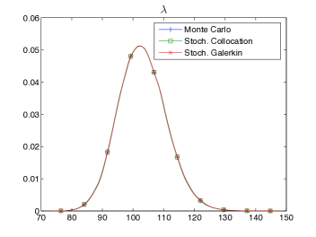
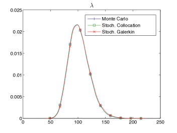
Fig. 2: Pdf estimates obtained from RQ⁽⁰⁾, for the minimal eigenvalue of the Timoshenko bean with $CoV=10\%$ (left) and $25\%$ (right).

First, we examine the performance of stochastic inverse iteration (SII) and compare it with stochastic collocation (SC). We ran stochastic inverse iteration with a fixed number of iterations, so plots of convergence indicators (31)–(34) shown below just illustrate the performance of the algorithms. We computed estimates of pdfs for the distributions of the eigenvalues and of the $\ell^{2}$-norm of the relative eigenvector error (33) corresponding to the minimal eigenvalue of the Timoshenko beam, with $CoV=10\%$ and 25%. Figure 2 shows the estimated eigenvalue distributions obtained using the “zero-step” computation (RQ⁽⁰⁾), which uses only the mean solution (18)–(19). The figure compares these distributions with those obtained using Monte Carlo and stochastic collocation, and it is evident that the visible displays of the three distributions are virtually indistinguishable. (Analogous plots, not shown, obtained after one complete stochastic iteration produced essentially identical plots.) As expected, the pdf estimates are narrower for $CoV=10\%$. This computation is explored further in Tables 1 and 2, which show the first ten coefficients of the gPC expansion of the smallest eigenvalue obtained using RQ⁽⁰⁾, one step and 20 steps of stochastic inverse iteration, and stochastic collocation. It can be seen that RQ⁽⁰⁾ provides good estimates of the four coefficients corresponding to the mean ($d=0$) and linear terms ($d=1$) of the expansion (5), and a single SII step significantly improves the quality of the quadratic terms ($d=2$).

Table 1: The first ten coefficients of the gPC expansion of the smallest eigenvalue of the Timoshenko beam with $CoV=10\%$ using $0$, $1$ or $20$ steps of stochastic inverse iteration, or using stochastic collocation. Here $d$ is the polynomial degree and $k$ is the index of basis function in expansion (5).

$d$	$k$	RQ(0)	SII(1)	SII(20)	SC
0	0	103.0823	102.9308	102.9307	102.9319
1	1	5.7301	5.7231	5.7231	5.7220
	2	-4.7970	-4.7854	-4.7854	-4.7848
	3	2.1156	2.1075	2.1075	2.1072
2	4	0.2361	0.2144	0.2144	0.2142
	5	-0.2540	-0.2803	-0.2804	-0.2807
	6	0.0841	0.1523	0.1523	0.1523
	7	0.1873	0.1272	0.1271	0.1250
	8	-0.1437	-0.0507	-0.0506	-0.0507
	9	0.0961	-0.0372	-0.0373	-0.0382

Table 2: The first ten coefficients of the gPC expansion of the smallest eigenvalue of the Timoshenko beam with $CoV=25\%$ using $0$, $1$ or $20$ steps of stochastic inverse iteration, or using stochastic collocation. Here $d$ is the polynomial degree and $k$ is the index of basis function in expansion (5).

$d$	$k$	RQ(0)	SII(1)	SII(20)	SC
0	0	103.0823	102.1705	102.1670	102.1713
1	1	14.0453	13.9402	13.9402	13.9408
	2	-11.7568	-11.5862	-11.5859	-11.5848
	3	5.1830	5.0654	5.0651	5.0669
2	4	1.4284	1.2919	1.2918	1.2909
	5	-1.5368	-1.6766	-1.6767	-1.6764
	6	0.5090	0.9030	0.9032	0.9035
	7	1.1331	0.7533	0.7530	0.7529
	8	-0.8696	-0.2965	-0.2960	-0.2955
	9	0.5812	-0.2215	-0.2220	-0.2222

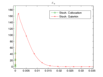
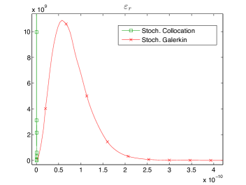
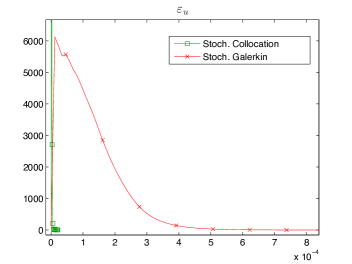
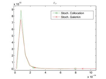
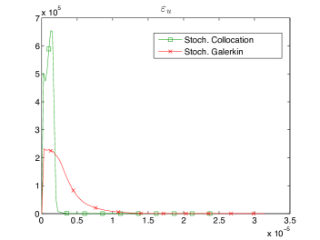
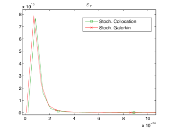
Fig. 3: Plots of the pdf estimate of the $\ell^{2}$-norms of the relative eigenvector error (33) (left) and the residual (34) (right) corresponding to the smallest eigenvalue of the Timoshenko beam with $CoV=10\%$ obtained using stochastic Rayleigh quotient RQ⁽⁰⁾ (top), and after stochastic inverse iteration $1$ (middle) and $2$ (bottom).

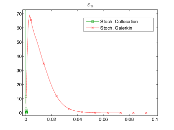
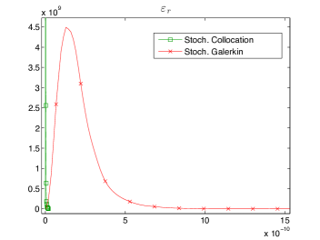
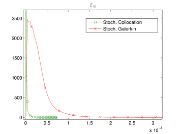
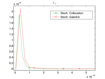
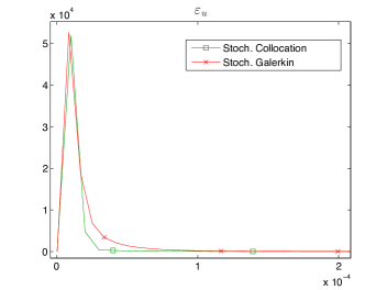
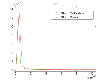
Fig. 4: Plots of the pdf estimate of the $\ell^{2}$-norms of the relative eigenvector error (33) (left) and the residual (34) (right) corresponding to the smallest eigenvalue of the Timoshenko beam with $CoV=25\%$ obtained using stochastic Rayleigh quotient RQ⁽⁰⁾ (top), and after stochastic inverse iteration $1$ (middle) and $2$ (bottom).

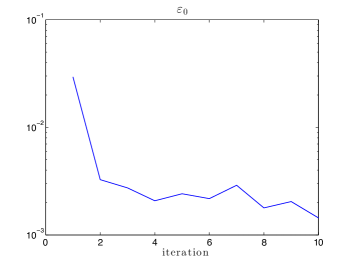
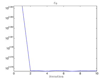
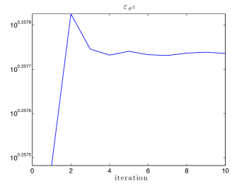
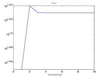
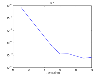
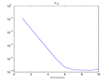
Fig. 5: Convergence history of convergence indicators (31) and (32) corresponding to the smallest eigenvalue of the Timoshenko beam with $CoV=10\%$ (left panels) and $CoV=25\%$ (right panels).

Analogous computations for eigenvector errors and eigenproblem residuals are summarized in Figures 3–4. These figures show estimates of pdfs for the eigenvector error (33) and the residual distribution (34) for the eigenvalue/eigenvector pair, corresponding to the smallest eigenvalue of the Timoshenko beam. The trends for convergence in both figures (corresponding to $CoV=10\%$ and $25\%$) are similar.

These figures provide insight into the maximal values of the errors (33) obtained from samples of the discrete eigenvectors. For example, in the display in the upper left of Figure 3, the support of the pdf for RQ⁽⁰⁾ (obtained from the mean solution) is essentially the interval $[0,0.02]$, which shows that the eigenvector error $\varepsilon_{u}$ from RQ⁽⁰⁾ is of order at most $2\%$. The analogous result for $CoV=25\%$ is $6\%$ (upper left of Figure 4), so that RQ⁽⁰⁾ is less accurate for the larger value of $CoV$. Nevertheless, it can be seen from Figure 4 that even with $CoV=25\%$, the eigenvector approximation error $\varepsilon_{u}$ is less than $0.15\%$ after one step of inverse iteration and after the second step $\varepsilon_{u}$ is less than $0.01\%$ and the error essentially coincides with the eigenvector error from stochastic collocation. In other words, the convergence of SII is also indicated by the “leftward” movement of the pdfs corresponding to $\varepsilon_{u}$. The pdf estimates of the residuals are very small after one inverse iteration. We also found that when the residual indicators (31) stop decreasing and the differences (32) become small, the sample true residuals (34) also become small. Figure 5 shows the behavior of the indicators (31)–(32).

Next, we consider the computation of multiple extreme eigenvalues. For the stochastic Galerkin method, this entails construction of the coefficients of $n_{s}>1$ eigenvalue fields in (24). The stochastic collocation method computes $n_{s}$ extreme eigenvalues for each sample point and then uses these to construct the random fields associated with each of them. Monte Carlo proceeds in an analogous way.

The performance of the methods for computing the five smallest eigenvalues of the Timoshenko beam with $CoV=25\%$ is shown in Figure 6. Stochastic Galerkin was able to identify the three smallest eigenvalues $\lambda_{1},\lambda_{2},\lambda_{3}$, but it failed to identify eigenvalues $\lambda_{4},\lambda_{5}$. (Results were similar for larger values of polynomial degree, $p=4$ and $5$.) Stochastic collocation and Monte Carlo were able to find all five eigenvalues. Note that the error indicators $\varepsilon_{0}$ and $\varepsilon_{\sigma}^{2}$ from (31), shown in the bottom of the figure, become flat for the converged eigenvalues but not for those that are not found. Performance results for the five largest eigenvalues are shown in Figure 7. The Galerkin method was robust in this case: for each of the five eigenvalues, the pdf estimates obtained by all three computational methods overlap, and the $\ell^{2}$-norm of the relative eigenvector error (33) corresponding to the fifth maximal eigenvalue is small. The error indicator $\varepsilon_{\sigma^{2}}$ from (31) behaves somewhat inconsistently in this case: after initial decrease it can be seen that $\varepsilon_{\sigma^{2}}$ increases slightly after approximately $85$ iterations.

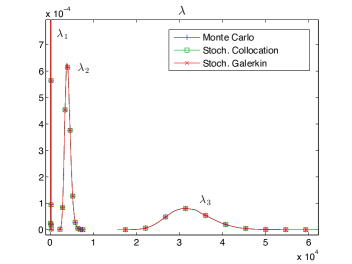
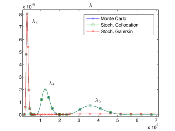
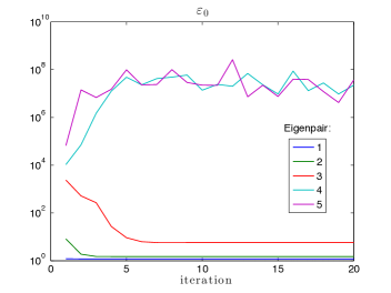
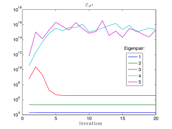
Fig. 6: Top: pdf estimates of the eigenvalue distribution corresponding to eigenvalues $\lambda_{1},\lambda_{2},\lambda_{3}$ (left) $\lambda_{3},\lambda_{4},\lambda_{5}$ (right). Bottom: convergence history of the two indicators $\varepsilon_{0}$ and $\varepsilon_{\sigma}^{2}$ from (31) obtained using inverse subspace iteration, for the five smallest eigenvalues of the Timoshenko beam with $CoV=25\%$.

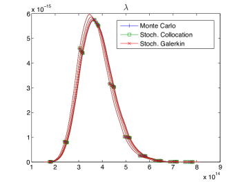
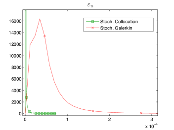
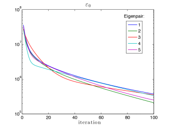
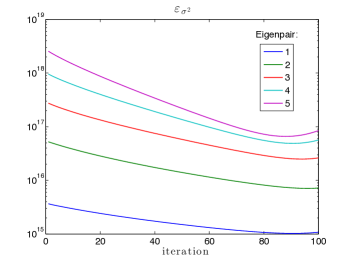
Fig. 7: Top: pdf estimates of the five largest eigenvalues of the Timoshenko beam with $CoV=25\%$ (left), and $\ell^{2}$-norm of the relative eigenvector error (33) (right). Bottom: convergence history of the two indicators $\varepsilon_{0}$ and $\varepsilon_{\sigma^{2}}$ from (31).

We explored several approaches to enhance the robustness of stochastic subspace iteration for identifying interior eigenvalues. One possibility is to use a shift. We tested inverse iteration with a shift to find the fifth smallest eigenvalue of the Timoshenko beam with $CoV=25\%$. The corresponding eigenvalue of the mean problem is $\overline{\lambda}_{5}=3.7548\times 10^{5}$. The top four panels in Figure 8 show plots of the pdf estimates of the eigenvalue distribution, the $\ell^{2}$-norm of the relative eigenvector error (33), the true residual (34), and the convergence history of the indicator$~{}\varepsilon_{0}$ from (31) with the shift$~{}\rho=4.1\times 10^{5}$. It can be seen that for the estimates of the pdfs of the eigenvalue, the relative eigenvector errors, and the true residual of the stochastic inverse iteration, the methods are in agreement. However, we also found that convergence depends on the choice of the shift $\rho$. Setting the shift far from the eigenvalue of interest or too close to it worsens the convergence rate and the method might even fail to converge. For this eigenvalue, the best convergence occurs with the shift set close to either $\rho=3.5\times 10^{5}$ or $\rho=4.1\times 10^{5}$, but with shift set to $\rho=3.9\times 10^{5}$ or $\rho=4.3\times 10^{5}$ the method fails to converge. Similar behavior was also reported in [29]. We note that the mean of the sixth smallest eigenvalue is $\overline{\lambda}_{6}=8.9196\times 10^{5}$, that is, the means of the fifth and sixth eigenvalues are well separated, see also Figure 1.

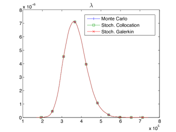
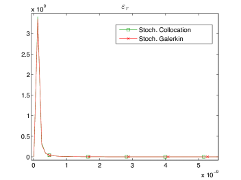
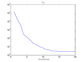
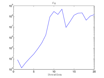
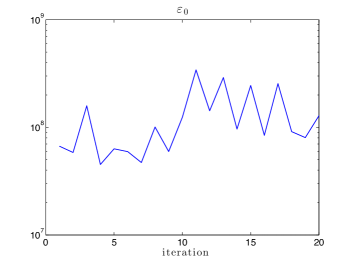
Fig. 8: Behavior of stochastic inverse iteration with shifts, for the fifth smallest eigenvalue of the Timoshenko beam, with $CoV=25\%$. Top: pdf estimates of the eigenvalue distribution (left) and $\ell^{2}$-norm of the relative eigenvector error (33) (right), obtained using shift $\rho=4.1\times 10^{5}$. Middle: pdf estimate of the true residual (34) (left) and convergence history of the indicator $\varepsilon_{0}$ from (31) (right), also with $\rho=4.1\times 10^{5}$. Bottom: stochastic inverse iteration fails to converge with shift $\rho=3.9\times 10^{5}$ (left) or $\rho=4.3\times 10^{5}$ (right), as illustrated by the convergence history of $\varepsilon_{0}$.

An approach that we found to be more robust was to use deflation of the mean matrix. Suppose we are interested in some interior eigenvalues in the lower side of the spectrum, for example $\lambda_{4}$ and $\lambda_{5}$, which we were unable to identify in a previous attempt (Figure 6). To address this, as suggested in (15) we can deflate the mean matrix $A_{0}$ using the mean eigenvectors corresponding to $\lambda_{1}$, $\lambda_{2}$ and $\lambda_{3}$. Figure 9 shows that in this case, Algorithm 2 was able to identify the fourth and fifth smallest eigenvalues, and the relative eigenvector errors (33) almost coincide. We note that the results in Figures 9 (and also in Figure 10) were obtained using the deflated mean matrix also in stochastic collocation and Monte Carlo methods.

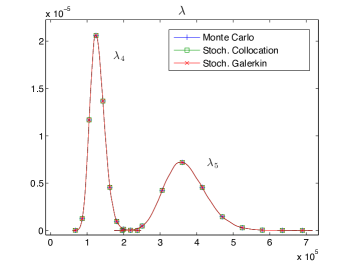
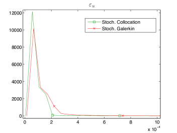
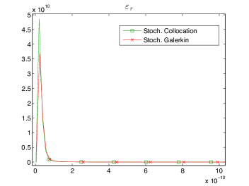
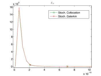
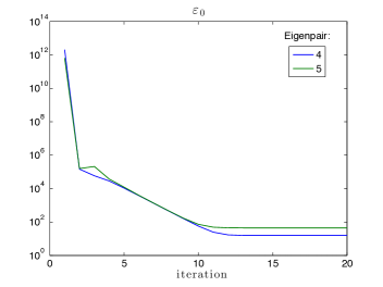
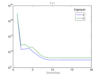
Fig. 9: Top: pdf estimates of the eigenvalue distribution $\lambda_{4}$ and $\lambda_{5}$ (left), and of the $\ell^{2}$-norm of the relative eigenvector error (33) corresponding to $\lambda_{5}$ (right). Middle: pdf of the $\ell^{2}$-norm of the true residual (34) corresponding to eigenvalues $\lambda_{4}$ (left), and $\lambda_{5}$ (right). Bottom: convergence history of the two indicators $\varepsilon_{0}$ and $\varepsilon_{\sigma}^{2}$ from (31) corresponding to eigenvalues $\lambda_{4}$ and $\lambda_{5}$ of the Timoshenko beam with $CoV=25\%$ obtained using inverse subspace iteration and deflation (15) of the three smallest eigenvalues $\lambda_{1}$, $\lambda_{2}$, and $\lambda_{3}$.

One significant advantage of stochastic inverse subspace iteration over Monte Carlo and stochastic collocation is that it allows termination of the iteration at any step, and thus the coefficients of the expansions (5) can be found only approximately. Figure 10 shows the $\ell^{2}$-norms of the relative eigenvector error (33) and the pdf estimates of the true residual (34) corresponding to the fifth smallest eigenvalue of the Timoshenko beam with $CoV=25\%$, obtained using inverse iteration with deflation of the four smallest eigenvalues in iteration $0$, $5$, and $10$. For example, the initial mean of the relative eigenvector error$~{}\varepsilon_{u}$ from  (33) is centered around $10\%$, after $5$ iterations it is reduced to less than $0.5\%$, and after $10$ iterations the results of stochastic inverse iteration and stochastic collocation essentially agree, and the difference from Monte Carlo represented by$~{}\varepsilon_{u}$ is less than $0.05\%$.

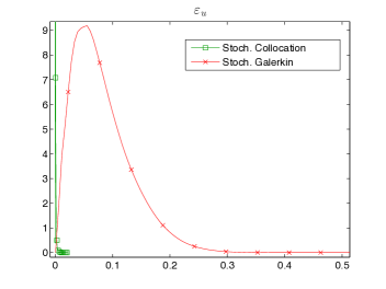
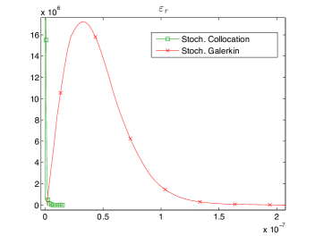
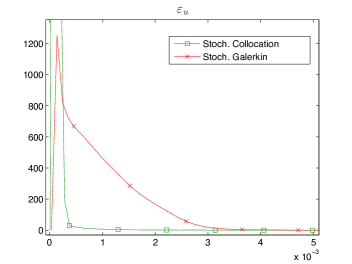
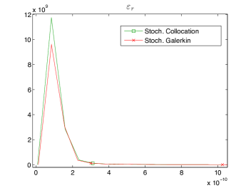
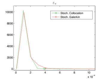
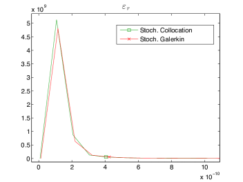
Fig. 10: Plots of the pdf estimate of the $\ell^{2}$-norms of the relative eigenvector error (33) and the true residual (34) corresponding to the fifth smallest eigenvalue of the Timoshenko beam with $CoV=25\%$ obtained using inverse iteration with deflation of the four smallest eigenvalues in iteration $0$ (top), $5$ (middle) and $10$ (bottom).

4.2 Example 2: Mindlin plate

For the second example, we analyzed vibrations of a square, fully simply supported Mindlin plate. For this problem we used $3\times 10^{4}$ Monte Carlo samples. The physical parameters were set according to [1, Section 12.5] as follows: the mean Young’s modulus of the lognormal random field was $E_{0}=10,920$, Poisson’s ratio $\nu=0.30$, length of a side $L_{\text{plate}}=1$, thickness $0.1$, $\kappa=5/6$, and density $\rho=1$. The plate was discretized using $10\times 10$ bilinear (Q4) finite elements with $243$ physical degrees of freedom. The condition number of the mean matrix$~{}A_{0}$ from (39) is$~{}1.6436\times 10^{3}$, the norm $\left\|A_{0}\right\|_{2}=1.8153\times 10^{7}$, and the eigenvalues of$~{}A_{0}$ are displayed in Figure 11. Coefficient of variation of the Young’s modulus was set to $CoV=25\%$, and the spatial correlation length $L_{corr}=L_{\text{plate}}/4$. This is a two-dimensional problem which means that there are repeated eigenvalues: for example, the four smallest eigenvalues of the mean problem are $\overline{\lambda}_{1}=1.1044\times 10^{4}$, $\overline{\lambda}_{2}=\overline{\lambda}_{3}=4.2720\times 10^{4}$, and $\overline{\lambda}_{4}=8.3014\times 10^{4}$.

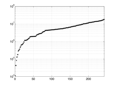
Fig. 11: Eigenvalues of the matrix $A_{0}$ corresponding to the Mindlin plate.

As before, we first examined the performance of stochastic inverse iteration and stochastic collocation to identify the smallest eigenvalue. The results are in Figure 12 and Table 3 presents a comparison of the first 10 coefficients of the gPC expansion of the smallest eigenvalue obtained using RQ⁽⁰⁾, one and five steps of stochastic inverse iteration, and stochastic collocation. Monte Carlo simulation gave sample mean $1.0952\times 10^{4}$ and standard deviation $1.2224\times 10^{3}$, i.e., $CoV\approx 11\%$. As before, RQ⁽⁰⁾ alone provides a close estimate of the eigenvalue expansion (5), and the results of stochastic inverse iteration and stochastic collocation essentially agree.

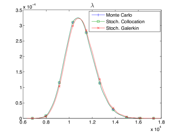
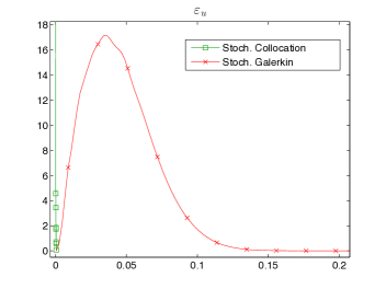
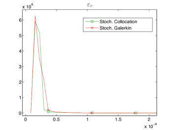
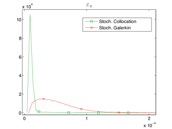
Fig. 12: Top: pdf estimates of the eigenvalue distribution (left) and the $\ell^{2}$-norm of the relative eigenvector error (33) (right) corresponding to the minimal eigenvalue $\lambda_{1}$ of the Mindlin plate with $CoV=25\%$ obtained directly using stochastic Rayleigh quotient RQ⁽⁰⁾. Bottom: pdf estimates of the true residual (34) (left) and of the relative eigenvector error (33) (right) after five steps of stochastic inverse iteration.

Table 3: The first ten coefficients of the gPC expansion of the smallest eigenvalue of the Mindlin plate with $CoV=25\%$ using $0$, $1$ or $5$ steps of stochastic inverse iteration, or using stochastic collocation. Here $d$ is the polynomial degree and $k$ is the index of basis function in expansion (5).

$d$	$k$	RQ(0)	SII(1)	SII(5)	SC
0	0	11,044.1637	10,960.2185	10,954.8258	10,954.8256
1	1	1227.0431	1217.0164	1216.3543	1216.3548
	2	0	0	0	0
	3	0	0	0	0
2	4	103.4832	97.6116	97.5149	97.5167
	5	0	0	0	0
	6	0	0	0	0
	7	40.8972	-15.9359	-19.7006	-19.6992
	8	0	0	0	0
	9	40.8972	-15.9359	-19.7006	-19.6992

Next, we used stochastic inverse subspace iteration to identify the four smallest eigenvalues. The results are in Figure 13. It can be seen that the distributions of all four eigenvalues match and, in particular, the distributions of the repeated eigenvalues$~{}\lambda_{2}$ and$~{}\lambda_{3}$ overlap. However, it also appears that stochastic collocation exhibits some difficulties detecting the subspace corresponding to $\lambda_{2}$, whereas the distribution of$~{}\varepsilon_{r}$ corresponding to$~{}\lambda_{4}$ suggests that in this case stochastic inverse subspace iteration and stochastic collocation methods are in excellent agreement.

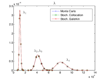
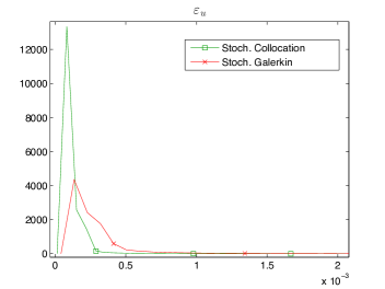
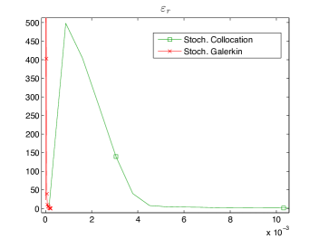
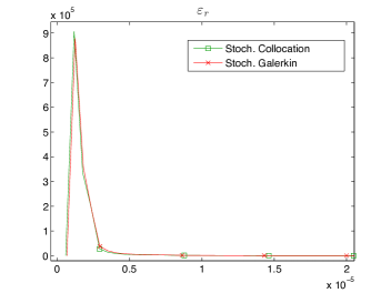
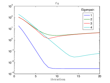
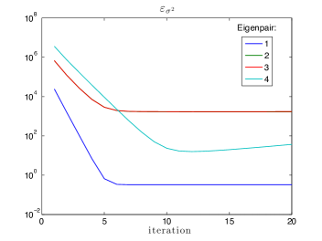
Fig. 13: Top: pdf estimates of the four smallest eigenvalues (left) and of the $\ell^{2}$-norm of the relative eigenvector error (33) corresponding to the fourth smallest eigenvalue of the Mindlin plate (right). Middle: pdf estimates of the true residual (34) corresponding to the second (left) and fourth (right) eigenvector. Bottom: convergence history of the two indicators $\varepsilon_{0}$ and $\varepsilon_{\sigma^{2}}$ from (31).

5 Conclusion

We studied random eigenvalue problems in the context of spectral stochastic finite element methods. We formulated the algorithm of stochastic inverse subspace iteration and compared its performance in terms of accuracy with stochastic collocation and Monte Carlo simulation. While overall the experiments indicate that in terms of accuracy all three methods are quite comparable, we also highlighted some differences in their methodology. In the stochastic inverse subspace iteration we formulate and solve a global stochastic Galerkin problem in order to find the coefficients of the gPC expansion of the eigenvectors. The coefficients of the eigenvalue expansion are computed from a stochastic version of the Rayleigh quotient. In fact, we found that the coefficients of the eigenvector expansion corresponding to the underlying mean-value problem, with the coefficients of the higher order terms set to zero, provide a good estimate of the probability distribution of the corresponding eigenvalue. From our experiments it also appears that the stochastic inverse subspace iteration is not robust when the nature of the eigenvalues is very different, for example, due to a badly conditioned problem. Moreover, the performance of inverse iteration for interior eigenvalues seems to be sensitive to the choice of the shift. Nevertheless, we were able to successfully resolve both issues by deflation of the eigenvalues of the mean matrix. The algorithm also performs well in cases when the spectrum is clustered and even for repeated eigenvalues. However, a unique description of stochastic subspaces corresponding to repeated eigenvalues, which would allow a comparison of different bases, is more delicate [8] and is not addressed here.

We briefly comment on computational cost. Stochastic inverse subspace iteration is a computational intensive algorithm because it requires repeated solves with the global stochastic Galerkin matrix. However, our main focus here was on the methodology, and we view a cost analysis to be beyond the scope of this project. In our experiments, we used direct solves for the global stochastic Galerkin system, and for deterministic eigenvalue problems required by the sampling (collocation and Monte Carlo) methods, we used the Matlab function eig. Many other strategies can be brought to this discussion, for example preconditioned Krylov subspace methods, e.g., [25, 26], to approximately solve the Galerkin systems, and state-of-the art iterative eigenvalue solvers for the sampling methods. Moreover, the solution of Galerkin systems is also a topic of ongoing study [16]. Finally, we note that an appealing feature of the Galerkin approach is that it allows solution of the random eigenvalue problem only approximately, performing zero (in case of the stochastic Rayleigh quotient) or only a few steps of the stochastic iteration, unlike the Monte Carlo and the stochastic collocation methods which are based on sampling.

Acknowledgement. We thank the two reviewers and the Associate Editor for careful readings of the manuscript and many helpful suggestions.

References

- [1] A. J. M. Ferreira, MATLAB Codes for Finite Element Analysis: Solids and Structures, Springer, 2009. (Solid Mechanics and Its Applications).
- [2] T. Gerstner and M. Griebel, Numerical integration using sparse grids, Numerical Algorithms, 18 (1998), pp. 209–232.
- [3] R. Ghanem, The nonlinear Gaussian spectrum of log-normal stochastic processes and variables, J. Appl. Mech., 66 (1999), pp. 964–973.
- [4] R. Ghanem and D. Ghosh, Efficient characterization of the random eigenvalue problem in a polynomial chaos decomposition, Int. J. Numer. Methods Eng., 72 (2007), pp. 486–504.
- [5] R. G. Ghanem and P. D. Spanos, Stochastic Finite Elements: A Spectral Approach, Springer-Verlag New York, Inc., New York, NY, USA, 1991. (Revised edition by Dover Publications, 2003).
- [6] D. Ghosh, Application of the random eigenvalue problem in forced response analysis of a linear stochastic structure, Archive of Applied Mechanics, 83 (2013), pp. 1341–1357.
- [7] D. Ghosh and R. Ghanem, Stochastic convergence acceleration through basis enrichment of polynomial chaos expansions, Int. J. Numer. Methods Eng., 73 (2008), pp. 162–184.
- [8] , An invariant subspace-based approach to the random eigenvalue problem of systems with clustered spectrum, Int. J. Numer. Methods Eng., 91 (2012), pp. 378–396.
- [9] H. Hakula, V. Kaarnioja, and M. Laaksonen, Approximate methods for stochastic eigenvalue problems, Applied Mathematics and Computation, 267 (2015), pp. 664–681.
- [10] M. E. Hochstenbach and G. L. Sleijpen, Two-sided and alternating Jacobi-Davidson, Linear Algebra Appl., 358 (2003), pp. 145–172.
- [11] R. A. Horn and C. R. Johnson, Topics in Matrix Analysis, Cambridge University Press, 1991.
- [12] M. Kamiński, The Stochastic Perturbation Method for Computational Mechanics, John Wiley & Sons, 2013.
- [13] M. Kleiber, The Stochastic Finite Element Method: Basic Perturbation Technique and Computer Implementation, Wiley, New York, 1992.
- [14] O. Le Maître and O. M. Knio, Spectral Methods for Uncertainty Quantification: With Applications to Computational Fluid Dynamics, Scientific Computation, Springer, 2010.
- [15] H. G. Matthies and A. Keese, Galerkin methods for linear and nonlinear elliptic stochastic partial differential equations, Comput. Meth. Appl. Mech. Eng., 194 (2005), pp. 1295–1331.
- [16] H. G. Matthies and E. Zander, Solving stochastic systems with low-rank tensor compression, Linear Algebra Appl., 436 (2012), pp. 3819–3838.
- [17] H. Meidani and R. G. Ghanem, A stochastic modal decomposition framework for the analysis of structural dynamics under uncertainties, in Proceedings of the 53rd Structures, Structural Dynamics, and Materials Conference, Honolulu, HI, 2012.
- [18] , Spectral power iterations for the random eigenvalue problem, AIAA Journal, 52 (2014), pp. 912–925.
- [19] M. P. Nightingale and C. J. Umrigar, Monte Carlo Eigenvalue Methods in Quantum Mechanics and Statistical Mechanics, John Wiley & Sons, 2007, pp. 65–115.
- [20] E. Novak and K. Ritter, High dimensional integration of smooth functions over cubes, Numer. Math., 75 (1996), pp. 79–97.
- [21] B. Pascual and S. Adhikari, Hybrid perturbation-Polynomial Chaos approaches to the random algebraic eigenvalue problem, Comput. Meth. Appl. Mech. Eng., 217-220 (2012), pp. 153–167.
- [22] H. Pradlwarter, G. Schuëller, and G. Szekely, Random eigenvalue problems for large systems, Computers & Structures, 80 (2002), pp. 2415–2424.
- [23] E. Sarrouy, O. Dessombz, and J.-J. Sinou, Stochastic analysis of the eigenvalue problem for mechanical systems using polynomial chaos expansion— application to a finite element rotor, J. Vib. Acoust., 134 (2012), pp. 1–12.
- [24] M. Shinozuka and C. J. Astill, Random eigenvalue problems in structural analysis, AIAA Journal, 10 (1972), pp. 456–462.
- [25] B. Sousedík and R. G. Ghanem, Truncated hierarchical preconditioning for the stochastic Galerkin FEM, International Journal for Uncertainty Quantification, 4 (2014), pp. 333–348.
- [26] B. Sousedík, R. G. Ghanem, and E. T. Phipps, Hierarchical Schur complement preconditioner for the stochastic Galerkin finite element methods, Numerical Linear Algebra with Applications, 21 (2014), pp. 136–151.
- [27] L. Trefethen, Is Gauss quadrature better than Clenshaw–Curtis?, SIAM Review, 50 (2008), pp. 67–87.
- [28] L. N. Trefethen and D. Bau III, Numerical Linear Algebra, SIAM, 1997.
- [29] C. V. Verhoosel, M. A. Gutiérrez, and S. J. Hulshoff, Iterative solution of the random eigenvalue problem with application to spectral stochastic finite element systems, Int. J. Numer. Meth. Engng, 68 (2006), pp. 401–424.
- [30] J. vom Scheidt and W. Purkert, Random eigenvalue problems, North Holland series in probability and applied mathematics, North Holland, New York, 1983.
- [31] M. Williams, A method for solving a stochastic eigenvalue problem applied to criticality, Annals of Nuclear Energy, 37 (2010), pp. 894–897.
- [32] , A method for solving stochastic eigenvalue problems, Applied Mathematics and Computation, 215 (2010), pp. 3906–3928.
- [33] , A method for solving stochastic eigenvalue problems II, Applied Mathematics and Computation, 219 (2013), pp. 4729–4744.
- [34] D. Xiu, Numerical Methods for Stochastic Computations: A Spectral Method Approach, Princeton University Press, 2010.
- [35] D. Xiu and G. E. Karniadakis, The Wiener-Askey polynomial chaos for stochastic differential equations, SIAM J. Sci. Comput., 24 (2002), pp. 619–644.