Testing a thermo-chemo-hydro-geomechanical model for gas hydrate bearing sediments using triaxial compression lab experiments

Abstract

Natural gas hydrates are considered a potential resource for gas production on industrial scales. Gas hydrates contribute to the strength and stiffness of the hydrate-bearing sediments. During gas production, the geomechanical stability of the sediment is compromised. Due to the potential geotechnical risks and process management issues, the mechanical behavior of the gas hydrate-bearing sediments needs to be carefully considered. In this study, we describe a coupling concept that simplifies the mathematical description of the complex interactions occuring during gas production by isolating the effects of sediment deformation and hydrate phase changes. Central to this coupling concept is the assumption that the soil grains form the load-bearing solid skeleton, while the gas hydrate enhances the mechanical properties of this skeleton. We focus on testing this coupling concept in capturing the overall impact of geomechanics on gas production behavior though numerical simulation of a high-pressure isotropic compression experiment combined with methane hydrate formation and dissociation. We consider a linear-elastic stress-strain relationship because it is uniquely defined and easy to calibrate. Since, in reality, the geomechanical response of the hydrate bearing sediment is typically inelastic and is characterized by a significant shear-volumetric coupling, we control the experiment very carefully in order to keep the sample deformations small and well within the assumptions of poro-elasticity. The closely co-ordinated experimental and numerical procedures enable us to validate the proposed simplified geomechanics-to-flow coupling, and set an important precursor towards enhancing our coupled hydro-geomechanical hydrate reservoir simulator with more suitable elasto-plastic constitutive models.

Key points

1. A simplified coupling concept is proposed for modelling geomechanical feedback on gas production behaviour of hydrate reservoirs.

2. Coupling concept is validated by numerical simulation of gas hydrate formation and dissociation in a controlled triaxial compression test.

3. Coupling concept applies to pore-filling hydrates as well as for hydrates in the transition zone between pore-filling and load-bearing habits.

1 Introduction

Methane hydrates are crystalline solids formed from water molecules enclathrating methane molecules. Methane hydrates are thermodynamically stable under conditions of low temperatures and high pressures. If warmed or depressurized, methane hydrates destabilize and dissociate into water and methane gas. Natural gas hydrates occur in permafrost regions and the deep sea, usually in soils or sediments at considerable depth when methane is available in sufficient amounts. Natural gas hydrates are considered to be a promising energy resource. It is widely believed that the energy content of methane occurring in hydrate form is immense, possibly exceeding the combined energy content of all other conventional fossil fuels ([55], [8], [3], [43], [35]).

Several methods have been proposed for production of natural gas from gas hydrate reservoirs, e.g., thermal stimulation, depressurization, and chemical activation ([49, 50], [53], [36]). Currently, depressurization is deemed the most mature approach. Consequently, significant research and development effort has been directed towards assessing the potential of depressurization as a primary driving force for natural gas production from gas hydrate reservoirs. Recent field trials, onshore below the Alaskan permafrost and in the Nankai Trough offshore Japan were both essentially depressurization tests; the Japanese test used only depressurization ([77, 78], [12]), while, the Alaskan test was combined with $N_{2}$:$CO_{2}$ injection ([2], [63]).

In the earlier gas production studies, several mathematical models (e.g. [71], [1], [79], [68], [40], [48, 51]) and numerical simulators (e.g. MH21-HYDRES [34], STOMP-HYD [76], UMSICHT HyRes [26], TOUGH-HYDRATE [52]) were developed, which focused on hydrate phase change and fluid flow rather than on the geomechanical behaviour. Over the years, it has become increasingly clear that the geomechanical effects associated with these gas production methods cannot be ignored. Recent field trials have shown that large deformation and sand production are relevant risks for natural gas production from gas hydrate-bearing sediments ([63], [77, 78]), and reliable simulation tools are needed for risk assessment and production strategy development. Coupling between solid deformation and fluid transport lays the foundation for the simulation of the thermo-hydro-chemo-mechanical behavior of gas hydrate-bearing sediment during gas production, and the experimental validation of the coupling relationships is extremely important for adding certainty to predictive simulation of production scenarios and sediment mechanical behavior in general. Several mathematical and numerical tools (e.g., [32], [31], [59], [25], [20]) have since been developed to study gas production in gas hydrate reservoirs in a coupled thermo-chemo-hydro-geomechanical framework.

In a typical gas hydrate reservoir, the structure of the sediment is expected to change due to two distinct effects: 1) the changing hydrate saturation, and 2) the sediment deformation. What complicates the matter further is that the hydrate provides additional strength to the sediment through a cementation-like effect, thereby, effectively coupling the two inputs; hydrate saturation, and sediment deformation. For any detailed hydro-geomechanical description of the gas production from gas hydrate-bearing sediments, it is imperative to analyze how the transport processes (i.e., flow and chemical processes) would respond to any given geomechanical input. As can be expected, this is a rather challenging task due to the complexity of the interactions. In our model, we simplify the mathematical description of the coupled hydro-geomechanical processes by conceptualizing that the model can be decomposed into two distinct model blocks: transport-block and geomechanics-block, with the coupling between the two manifesting as changes in properties of each model block. (See Fig. 1.) The transport-block solves for the hydrate phase change and the non-isothermal, two-phase, two-component flow of water and methane gas, while the geomechanics-block solves for the sediment displacements. This decomposition is based on the simplifying assumption that the soil grains constitute the skeleton of the porous matrix, while the gas hydrate enhances the mechanical properties of this skeleton without actively bearing the load. The relative deformation of the gas hydrate phase with respect to the soil skeleton is ignored. This assumption allows us to distinguish between the total porosity and the apparent porosity. The total porosity characterizes the total pore volume, i.e. the volume not occupied by the soil grains, while the apparent porosity characterizes the actual pore volume which is available for the fluid flow. The deformation of the hydrate-bearing sediment directly affects only the total porosity. The evolution of the actual or apparent porosity field is then modelled by scaling the total porosity with functions of hydrate saturation through simple geometric arguments. To make the physical meaning clear, the apparent porosity is the actual measured quantity, while the total porosity is a mathematical construct which allows us to isolate the effects of sediment deformation from those of hydrate phase change. We also assume that those properties of the transport-block which depend on the sediment structure (i.e., hydraulic properties like permeability, capillary pressure, specific surface area, tortuosity etc.) can be modelled as a multiplicative decomposition of functions of total porosity and hydrate saturation. In effect, with these simplifications, we can describe all feedback from geomechanics-block to the transport-block through a single transfer variable: total porosity, and this forms a central feature of our coupling concept.

In this study, through numerical simulation of a highly controlled high-pressure triaxial experiment combined with methane hydrate formation and dissociation, we aim to establish whether this coupling concept is effective in capturing the overall impact of geomechanics on the gas production behaviour.

To be able to test the coupling with confidence, there are two important pre-requisites: 1) a well-tested model for the transport-block, and 2) a good enough estimation of the displacement field. The validation of the transport-block in our hydrate reservoir model was performed in our earlier study ([20]). For the second pre-requisite, however, we require a suitable constitutive model for describing the stress-strain response of the hydrate-bearing sediment. A number of non-linear elastic (e.g. [80, 46, 47]), elasto-plastic (e.g. [32, 72, 69, 39]), and elasto- viscoplastic (e.g. [31]) constitutive models have been proposed in the recent years to model the geomechanical behaviour of gas hydrate-bearing sediments. The stress strain relation in these models is quite complex. Variationally consistent formulations result in non-linear and non-smooth inequality settings. These can be reformulated in terms of non-linear complementarity functions to which semi-smooth Netwon algorithms as iterative solvers can be applied, which converge locally. To enlarge the local convergence radius, suitable regularisation and damping strategies can be designed ([22, 21]). Only in special situations existence and uniqueness is given, and often, only local existence is guaranteed and path dependent solutions exist. We refer to [41, 42] and the references therein for existence results at finite strain. However, none of these results can be directly applied to our setting since we have a fully coupled hydrate system involving more non-linearities in the bi-directional couplings. Additionally, the constraints of the system involve inequalities which are nonlinear and non-smooth, leading to a model with a large number of parameters which often makes model calibration challenging and unreliable. To the best of our knowledge, none of these models have been validated in coupled hydro-geomechanical settings in the context of gas production from gas hydrate reservoirs, and have a large uncertainty associated with their predictive capabilities in highly dynamic conditions. In this study, it is of particular interest to reduce the complexity of the geomechanics-block as much as possible in order to reduce the uncertainty associated with the choice of a constitutive model. We, therefore, chose a uniquely invertible linear-elastic constitutive model in the geomechanics-block of our hydrate reservoir model. We account for the stiffening effect due to gas hydrates by parameterizing the Young’s modulus as a function of hydrate saturation $S_{h}$ ([62]). We also account for material compressibility with respect to hydrostatic pressure. The pressure dependence of compressibility and the $S_{h}$ dependence of Lame’s parameters introduces a weak nonlinearity in the geomechanics-block. The numerical implementation of the poro-elastic model and the transport-to-geomechanics coupling in our hydrate reservoir model was also validated in our earlier study ([20]).

In general, poro-elasticity is not a realistic model for the geomechanical description of cemented granular materials where the stress-strain response is typically non-linear, and the shear-volumetric coupling (dilatancy) is of particular importance. Therefore, in order to validate our coupling concept within the constraints stated above, we control our triaxial experiment very carefully in a way that ensures that the assumptions of poroelasticity remain valid throughout the periods of interest for numerical simulation.

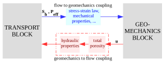
Figure 1: Coupling concept

2 Hydrate reservoir model

Mathematical model

Our model considers kinetic hydrate phase change and non-isothermal, multi-phase, multi-component fluid flow through poro-elastic porous medium. The model assumes that the porous medium is composed of three components: $CH_{4}$, $H_{2}O$ and methane hydrate ($CH_{4}\cdot{N_{h}}H_{2}O$), which are present in three distinct phases: gaseous, aqueous, and solid. The gaseous phase comprises of methane gas and water vapour. The aqueous phase comprises of water and dissolved methane. The solid phase comprises of pure methane hydrate and sand grains. The sand grains are assumed to form a material continuum which provides the skeletal structure to the porous medium. We shall refer to this as solid matrix. The aqueous, gaseous, and hydrate phases exist in the void spaces of this solid matrix (See Fig.2).

We assume that the hydrate cements the sand grains in the mechanical sense (i.e., without forming any chemical bonds), such that the sand and hydrate together form a composite solid matrix. The relative deformation of the gas hydrate phase with respect to the soil skeleton is ignored. This assumption allows us to write a single momentum balance equation for the composite solid phase, instead of separate ones for the sand and the hydrate phases each. To describe the mechanical behaviour of the composite solid matrix, we make a further simplifying assumption that the sand grains form the primary load-bearing structure, while the hydrates enhance the mechanical strength and stiffness of this structure without bearing any load themselves. This assumption is also adopted even after hydrate-bearing soil is loaded during depressurization. Because of this, the constitutive law does not consider stress-relaxation term that accounts for the release of load that has been carried by hydrates as introduced by others ([32, 72]).

We decompose the mathematical model into transport and geomechanics blocks, and isolate the effects of hydrate phase change and ground deformation through the introduction of the variable total porosity. This is justified based on the above assumption that the soil grains constitute the primary load-bearing skeleton of the porous matrix, such that deformation of the hydrate-bearing sediment directly affects only the total porosity. This assumption allows us to solve for the mass balance of soil and hydrates separately, thus conveniently separating hydrate phase change kinetics from sediment deformation. If, for example, we do not make this assumption, then we would have to solve for the mass balance of soil and hydrate as a single composite phase leading to a strong coupling between hydrate phase change and geomechanics. The model decomposition would not be straightforward in this case, and the evolution of porosity field would be very complex, making the description of the fluid flow and the evolution of the hydraulic properties also significantly more challenging. One clear advantage of this simplification is that it gives a very modular structure to the model, with each model-block operating independently, and communicating with each other through coupling relationships which are neatly resolved with respect to the independent output variables of each model-block. (See Fig. 1.) Another important advantage is that the model decomposition allows us to use multi-rate time-stepping schemes, as discussed in [19], which can significantly speed up the calculation, especially for 3D problems.

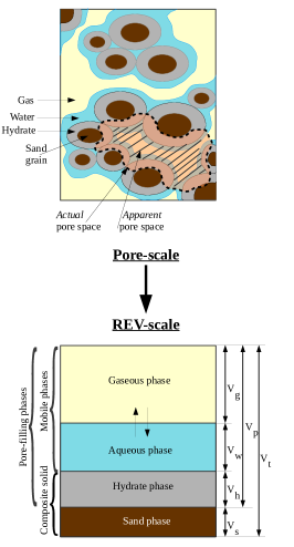
Figure 2: Pore-scale to REV-scale

The mathematical model is described in detail in [20]. A summary of the governing equations and the constitutive relationships is given in Table LABEL:table:modelSummary. The phases occupying the pore space (gaseous, aqueous, hydrate) are denoted by ’$\beta$’ $=g,w,h$ respectively, the mobile phases (gaseous and aqueous) are denoted by ’$\alpha$’ $=g,w$, and the mobile molecular components are denoted by ’$\kappa$’ $=CH_{4},H_{2}O$. The solid matrix is designated with the subscript ’$s$’. The sand+hydrate composite solid matrix is designated with the subscript ’$sh$’. ’$\gamma$’ is used to denote all phases, i.e., $\gamma=g,w,h,$ and $s$.

Primary variables

The mathematical model consists of the following $6$ governing equations: the mass balance Eqns. (LABEL:eqn:MassBal_g,LABEL:eqn:MassBal_w,LABEL:eqn:MassBal_h,LABEL:eqn:MassBal_s), the momentum balance Eqn. (LABEL:eqn:MomentumBal_sh) for the composite-solid, and the energy balance Eqn. (LABEL:eqn:EnergyBal). The momentum balance Eqns. (LABEL:eqn:Darcy_g,LABEL:eqn:Darcy_w) for the mobile phases $\alpha=g,w$ give the $\alpha-$phase velocities directly, and are thus absorbed in the mass and energy balance equations. We chose the following set of variables as the primary variables: the gas phase pressure $P_{g}$, the aqueous phase saturation $S_{w}$, the hydrate phase saturation $S_{h}$, the temperature $T$, the total-porosity $\phi$, and, the composite-matrix displacement $\mathbf{u}$. All other variables can be derived (explicitly or implicitly) from this set of variables using the closure and constitutive relationships.

Solution strategy

We use an iteratively coupled solution strategy. The mathematical model is decomposed into three parts:

1. transport-block ($\mathbf{F_{f}}$), comprised of the mass balance equations for $CH_{4}$, $H_{2}O$, and Hydrate, and the energy balance equation,

2. geomechanical-block ($\mathbf{F_{g}}$), comprised of the momentum balance equation for composite solid phase, and

3. porosity-equation ($\mathbf{F_{\phi}}$), comprised of the mass balance equation for the sand phase.

$\mathbf{F_{f}}$ is solved for the variables $P_{g}$, $S_{w}$, $S_{h}$, and $T$, $\mathbf{F_{g}}$ is solved for displacements $\mathbf{u}$, and $\mathbf{F_{\phi}}$ is solved for total porosity $\phi$. $\mathbf{F_{f}}$ and $\mathbf{F_{\phi}}$ are spatially discretized using a fully upwinded cell centered finite volume method. Orthogonal grids aligned with the principal axes are defined and a control-volume formulation with two-point flux approximation (TPFA) is used. $\mathbf{F_{g}}$ is discretized using Galerkin finite element (FEM) method defined on $Q1$ elements. An implicit Euler time-stepping scheme is used for marching forward in time. The solution for a given time step involves two iterative loops, the inner loop and the outer loop. The inner loop uses Newton’s method and SuperLU ([14]) linear solver to solve each of $\mathbf{F_{f}}$, $\mathbf{F_{g}}$, and $\mathbf{F_{\phi}}$, thus taking care of the decoupled solution. The outer loop re-introduces the coupling between $\mathbf{F_{f}}$, $\mathbf{F_{g}}$, and $\mathbf{F_{\phi}}$ through a block Gauss Seidel iterative scheme.

The numerical scheme is implemented in the C++ based DUNE-PDELab framework ([13]), and is capable of solving problems in $1D$, $2D$ and $3D$ domains.

3 Material and Methods

We performed a controlled triaxial volumetric strain test on a sand sample in which methane hydrate was first formed under controlled effective stress and then dissociated via depressurization under controlled total stress. Gas hydrate in our experiment was initially formed by pressurizing partially water-saturated sand with gaseous methane to reach a gas hydrate saturation of $0.4$, and remaining methane gas was replaced with seawater before the sample was depressurized stepwise. Confining and axial loads in the triaxial testing were applied isotropically and were carefully controlled to keep the deformation of the sample small and well within the assumptions of poroelasticity.

Experimental set-up and components

Experiments were carried out in the custom-made high-pressure apparatus NESSI (Natural Environment Simulator for Sub-seafloor Interactions, [16]), which is equipped with a triaxial cell mounted in a $40$ L stainless steel vessel (APS GmbH Wille Geotechnik, Rosdorf, Germany). The sample sleeve is made from FKM, other wetted parts of the setup are made of stainless steel. Salt water medium was stored in reservoir bottles (DURAN, Wertheim, Germany) prior to use in experiments, and the seawater medium was pressurized in an additional pressure vessel (Parr Instrument GmbH, Frankfurt, Germany) to allow fast transfer into the sample vessel. Fluid pressure in the sample vessel was adjusted with a back-pressure regulator valve (TESCOM Europe, Selmsdorf, Germany). Experiments were carried out in upflow mode with injection of $CH_{4}$ gas and seawater medium at the bottom of the sample prior to and after gas hydrate formation (Fig.3-a), respectively, and fluid discharge at the top of the sample during depressurization (Fig.3-b). Axial and confining stresses, and the sample volume changes were monitored throughout the experimental period. Axial and confining stresses were controlled using high-precision hydraulic pumps and actuators (VPC $400$, APS GmbH Wille Geotechnik, Rosdorf, Germany), and changes in hydraulic fluid volumes were converted to calculate sample volume changes. Pore pressure was measured in the influent and the effluent fluid streams close to the sample top and bottom. The experiment was carried out under constant temperature conditions. Temperature control was achieved with a thermostat system (T1200, Lauda, Lauda-Königshofen, Germany). Produced gas mass flow was analyzed with mass flow controllers (EL FLOW, Bronkhorst, Kamen, Germany). For control purposes, bulk effluent fluids were also collected inside $100$ L gas tight TEDLAR sampling bags (CEL Scientific, Santa Fe Springs CA, USA). The sampling bags were mounted inside water filled containers. After expansion of the effluent fluids at atmospheric pressure, the overall volume was measured as volume of water displaced from these containers.

Sample preparation and mounting

The sediment sample was prepared from quartz sand (initial sample porosity: $0.35$, grain size: $0.1-0.6$ mm, G20TEAS, Schlingmeier, Schwülper, Germany), which was mixed with de-ionized water to achieve a final water saturation of $0.4$ relative to the initial sample porosity. The partially water-saturated and thoroughly homogenized sediment was filled into the triaxial sample cell to obtain final sample dimensions of $360$ mm in height and $80$ mm in diameter. The sample geometry was assured using a sample forming device. The sample was cooled to $2^{0}$C after the triaxial cell was mounted inside the pressure vessel. Initial water permeability of the gas hydrate-free sediment was estimated to be $5\times 10^{-10}$ $m^{2}$ .

Experimental procedure

a) Gas hydrate formation

Prior to the gas hydrate formation, the partially water-saturated sediment sample was isotropically consolidated to $1$ MPa effective stress under drained conditions. It should be noted, that the apparent effective stress is monitored and controlled as differential pressure between the confining hydraulic fluid pressure of the reactor and the gas pressure in the sample pore space. Measurements and control algorithms do not take into account the changes in effective stress due to changes in water saturation and capillary pressure. Thus, only the apparent effective stress is directly accessible from experimental procedures. The sample was flushed with $CH_{4}$ gas to replace air with methane. The sample was, subsequently, pressurized with $CH_{4}$ gas to approximately $12.5$ MPa (Fig.3-a). During pressurization with $CH_{4}$ gas and throughout the overall gas hydrate formation period, formation stress condition of $1$ MPa effective stress were maintained using an automated control algorithm. The formation process was continuously monitored by logging the $CH_{4}$ gas pressure. Mass balances and volume saturations were calculated based on $CH_{4}$ gas pressure and initial mass and volume values. Gas hydrate formation was terminated after $1.84$ mol of $CH_{4}$-hydrate had been formed after approximately $6$ days, corresponding to CH4-hydrate saturation of $0.39$. The sample was cooled to $-5^{0}$C and stress control was switched to constant total isotropic stress control at approximately $9$ MPa before the sample pore space was de-pressurized to atmospheric pressure and the remaining $CH_{4}$ gas in the pore space was released. System re-pressurization and water saturation of the pore space was achieved by instant filling and re-pressurization with pre-cooled $-1^{0}$C saltwater medium according to the seawater composition. Hydrate dissociation during the brief period of depressurization was minimized by taking advantage of the anomalous self-preservation effect, which reaches an optimum close to the chosen temperature ([66]). After completion of the gas-water fluid exchange, the sample temperature was re-adjusted to $2^{0}$C.

b) Depressurization and gas production

The sample pore space was de-pressurized and gas produced by stepwise decrease of back pressure at constant isotropic total stress (Fig.3-b). Overall fluid production (water and $CH_{4}$ gas) was monitored after de-pressurization at atmospheric pressure after temperature equilibration.

a) Gas hydrate formation.

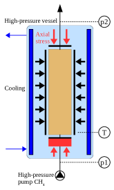
b) Depressurization and gas production.

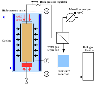
Figure 3: Simplified flow schemes for relevant period.

4 Numerical Simulation

The overall experiment was carried out in four steps, viz. 1) pre-consolidation, 2) gas hydrate formation, 3) pore-fluid exchange, and 4) depressurization, as described in section 3. During steps $1$ and $2$, the sample was maintained under a defined effective loading with the confining and the axial stresses were controlled to remain $10$ bar above the pore pressure. During steps $3$ and $4$, the total isotropic stress was controlled to remain at a constant level. (See Fig. 4.) The experiment was performed over a total period of about $16.8$ days. The periods of interest for this simulation are: 1) from $Day-3$ to $Day-10$, corresponding to gas hydrate formation, and 2) from $Day-12.8$ to $Day-13.8$, corresponding to depressurization and gas production. We simulate both of these periods separately.

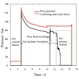
Figure 4: Overview of the measured pressure and stresses over time.

Computational domain

Assuming that the sand sample is axially symmetric, a $2D$ radial plane of dimensions $360$ mm $\times$ $40$ mm is chosen as the computational domain. The dimensions correspond to the physical size of the sample. The domain is discretized into $72\times 8$ cells.

Test-setting

a) Gas hydrate formation period

The schematic of the hydrate formation test is shown in Fig.5. The schematic also shows the initial and boundary conditions. The simulation is run until $t_{end}=604800$ s (i.e. $7$ days) using a maximum time step size of $120$ s.

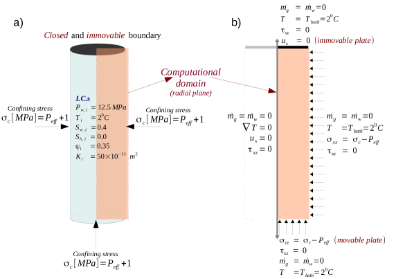
Figure 5: Test setting for the gas hydrate formation period.
a) shows the sample and the initial conditions, and b) shows the $2D$ computational domain and the boundary conditions.

b) Depressurization and gas production period

The schematic of the depressurization test is shown in Fig.6. The schematic also shows the initial and boundary conditions. The simulation is run until $t_{end}=86400$ s (i.e. $1$ day) using a maximum time step size of $120$ s.

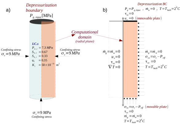
Figure 6: Test setting for the depressurization and gas production period.
a) shows the sample and the initial conditions, and b) shows the $2D$ computational domain and the boundary conditions.

Properties and parameters

The material properties and model parameters chosen for this simulation are listed in Table LABEL:table:materialProperties. The values of the thermal conductivities, specific heat capacities, dynamic viscosities, and densities for each phase are chosen from standard literature, the references to which are included in the table. The Brooks-Corey parameters are chosen from the range of typically expected values for sand samples.

The most important properties and parameters relevant to the simulation of the experimental data arise from 1) the hydrate-phase-change kinetics, and 2) the poro-elastic behaviour of the hydrate bearing sediments.

The hydrate phase-change is modelled by Eqns. (LABEL:eqn:GasGenRate,LABEL:eqn:WaterGenRate-LABEL:eqn:HeatOfReaction). The hydrate-phase equilibrium pressure $P_{e}$ in Eqn. LABEL:eqn:GasGenRate is modelled in accordance with the findings of [29]. For hydrates in pure water, the equilibrium pressure depends only on the temperature. However, for hydrates in sea water (which is the case for our sample), the equilibrium pressure also depends on the salinity, as shown in Fig.7. We account for the effect of salinity on the hydrate equilibrium pressure through linear curve fitting on dissociation pressure vs. salinity curve.

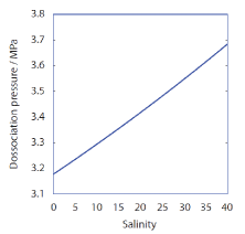
Figure 7: Effect of salinity on hydrate stability curve (at $T_{bath}=2^{0}C$)

a) Average gas pressure $P_{g}$ in the domain over time.

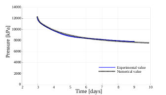
b) Average $S_{w}$ and $S_{h}$ in the domain over time.

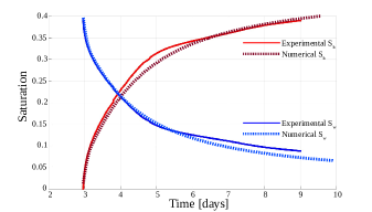
c) Total volumetric strain in the sample over time.
note: ’+’ value indicates compression.

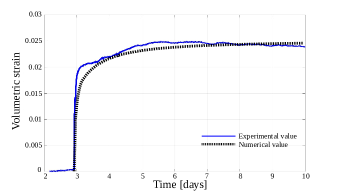
Figure 8: Comparison of the simulation results with the experimental results for the gas hydrate formation period.

The reaction surface area, $A_{rs}$, in Eqn. LABEL:eqn:GasGenRate, describes the surface area available for the kinetic-reaction, and puts a limit on the mass transfer during hydrate formation and dissociation. As the hydrate saturation in the pore-space increases, the availability of free surface for hydrate formation to occur decreases, and vice versa. Additionally, for hydrate formation, availability of both gas and water in sufficient quantities in the pore-space is a necessary condition. This behaviour of $A_{rs}$ is modelled using the parameterization proposed by [67].

The rate of reaction, $k_{reac}$, is a free parameter in our simulation which is used to calibrate the hydrate-kinetics model with respect to the experimental data. In the table we can see that the values of $k_{reac}$, for both hydrate formation as well as dissociation periods, lie well within the range reported in the literature.

The poro-elastic behaviour of the hydrate-bearing sediment is characterized by three parameters, viz., Biot’s constant $\alpha_{biot}$, Poisson ratio $\nu_{sh}$, and Young’s modulus $E_{sh}$. Biot’s constant is chosen from a range of typically expected values. The Poisson’s ratio is assumed to be a constant independent of the hydrate saturation following the experimental studies by [45, 38]. The Young’s modulus is modelled using the parameterization proposed by [62], given by Eqn. LABEL:eqn:Esh. The Young’s modulus $E_{sh}$ is a free parameter which are used to calibrate the poro-elasticity model with respect to the experimental data.

Simulation results

As discussed above, we essentially chose one free parameter in kinetics, i.e., $k_{reac}$, and one free parameter in linear-elasticity, which is $E_{sh}$, to calibrate the kinetic and the mechanical models separately. With these calibrated models, we simulate numerically the coupled (thermo-chemo)-hydro-geomechanical response of the sand sample in triaxial test-setting using our gas hydrate reservoir model. The numerical results, together with the corresponding experimental data, are plotted in Fig. 8 for the gas hydrate formation period, and in Fig. 9 for the hydrate dissociation period.

In the gas hydrate formation period, methane gas in the free pore space is continuously consumed and average bulk gas pressure is decreased. (See Fig. 8-a.) Clearly, the rate of gas hydrate formation is not constant. In the beginning, after the sample is pressurized at constant isotropic effective stress, gas hydrate formation from free methane gas and pore water is fast, but the rate of formation steadily decreases due to mass transfer limitations and shrinking reaction surfaces. In accordance to that, after pressurization the gas hydrate saturation increases rapidly and the water saturation decreases proportionally (Fig. 8-b). Note that the reported values of phase saturations are calculated based on initial values and gas pressure measurements. The volumetric strain shows a fast positive response during early gas hydrate formation at relatively low gas hydrate saturations, and sample stiffness increases at higher gas hydrate saturations (Fig. 8-c). The fast volumetric strain response that occurs at constant apparent effective stress results from changes in water saturation and, thus, capillary pressure, which is not monitored experimentally, but considered in the numerical simulation.

During the gas hydrate dissociation period, pressure is decreased step-wise until methane hydrates become unstable at the respective P-/T-conditions. Fig. 9-a shows the numerically computed gas phase pressure in the sample. The gas production is plotted in Fig. 9-b. With the onset of gas hydrate dissociation after reaching the hydrate stability boundary, pressure is maintained at a relatively constant level because hydrate dissociation and gas production equilibrate dependent on experimental and technical conditions.

Volumetric strain during gas hydrate dissociation, plotted in Fig. 9-c, is dependent on effective stress and gas hydrate saturation through the sample stiffness, which decreases with the ongoing gas hydrate dissociation and gas production.

Fig. 9-d shows the numerically computed temperature profile of the sample during dissociation. The model predicts that sub-cooling from gas hydrate dissociation is quite small, which is expected since the experiment was performed under isothermal temperature control.

a) Gas pressure $P_{g}$ at depressurization boundary (at $z=0$).

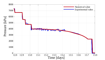
b) Cumulative gas production over time.

c) Total volumetric strain in the sample over time.
note: ’+’ value indicates compression.

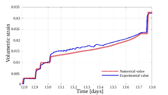
d) Temperature in the sample over time.

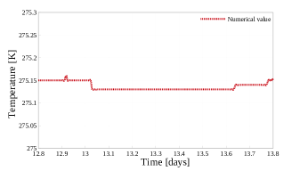
Figure 9: Comparison of the simulation results with the experimental results for the depressurization and gas production period.

5 Discussion and Outlook

In our combined experimental-numerical study, we consider dynamic gas hydrate formation and dissociation in sandy sediment under isotropic compressive loading and show that a simplified coupling concept is capable of reproducing the essential bulk physical behavior, including volumetric strain and gas production.

The assumption that the soil is the primary load-bearing constituent is central to our model concept. This assumption is most reasonable for the pore-filling hydrates with low satuations where the hydrates form by nucleating on sediment grain boundaries and grow freely into pore spaces without entering the pore-throats. For hydrates formed in partially water saturated sands, as is the case in our experiment, it is well known that the hydrates nucleate preferentially in the pore-throats and contribute to the sediment stiffness already at low gas hydrate saturations. For hydrate saturations between $0.25-0.4$, the hydrates are expected to transition towards a load-bearing habit [75]. In our experiment, we obtain a maximum hydrate saturation of $\approx 0.4$. Our numerical results suggest that in well consolidated sands, our assumption of soil forming the primary load-bearing skeleton remains valid even for hydrate saturations which lie in the transition zone between pore-filling and load-bearing habits. We hypothesize that this is because in well consolidated sands, the deformation of hydrates relative to the soil skeleton is quite small in the transition zone. However, for higher hydrate saturations where hydrates become fully load-bearing, we expect strong limitations to this coupling concept. Furthermore, for massive hydrates with saturations exceeding $0.8$, we even expect that the hydrate and the soil phases can no longer be modelled as a single composite phase, and new model concepts are necessary to consistently describe the interface conditions between the hydrate and the soil phase boundaries.

Our experiment was focused on analyzing deformation under variable gas hydrate saturation, and a wide range of effective stress loading, controlled between $1$ to $9$ MPa. To limit the bulk sample deformation and relative grain-to-grain movement only isotropic stresses were applied. Gas hydrates were formed after isotropic consolidation to $1$ MPa using the excess-gas-method ([10], [9], [27], [56]). After gas hydrate formation, the remaining gas was fully replaced with seawater. After gas-seawater replacement, the sample was equilibrated for approximately $5$ days to allow for gas hydrate alteration before the sample was depressurized. A poro-elasticity framework was chosen for describing the mechanical behavior of the sediment in order to minimize the uncertainties arising from unknown mechanical behavior of gas hydrate-bearing sediments. The deliberate choice of a simple constitutive law with a limited number of parameters, in contrast to using more complex elasto-plastic modeling approaches, is justified by the design of the experimental test case. It is important to note that, within the constraints of small-strain deformations and pore-filling hydrates, the coupling concept presented here does not depend on the stress-strain constitutive law as such. The concept of poro-elasticity is, therefore, sufficient to test the validity of our coupling concept provided that the design of the experiment ensures that the sample deformations remain small and well within elastic limit. For large deformations, the coupling concept is not validated so far.

To approximate our experimental data, we treated the kinetic term $k_{reac}$ in the transport block as a fitting parameter. Similarly, we used fitting of the stiffness model parameters to match the experimental volumetric strain behavior. We chose a functional dependence of composite modulus $E_{sh}$ on hydrate saturation $S_{h}$ as proposed by [62] and other authors ([60], [32, 33]). Knowledge about mechanical stiffness and strength properties of gas hydrate-bearing sediments is still limited. Experimental analysis of mechanical properties is problematic, because it is equally important to control effective stress conditions and phase saturations, and there are no test procedures available to guarantee homogeneous gas hydrate saturations and full water saturation. Further, mechanical properties are strongly dependent on gas hydrate-sediment fabrics and formation procedures, and effects from dynamic changes in gas hydrate saturation, distributions and alterations of gas hydrate-sediment fabrics needs further investigation and development of novel test procedures ([15]) particularly for dynamic test scenarios. Overall, the calibrated values for $E_{sh}$ from our study are in accordance with earlier experimental and numerical studies, which reported Young’s modulus or secant stiffness in a wide range of approximately $100$ to $400$ MPa for relevant gas hydrate concentrations ([6], [44], [37], [81]). Although the composite modulus $E_{sh}$ was treated as a free fitting parameter and initialized based on apparent stress-strain behavior during the intervals of known and constant gas hydrate saturations, physically meaningful values for individual modulii $E_{s}$ and $E_{h}$ were obtained. $E_{s}$ for the sediment without gas hydrate reflected stiffness behavior typical for loose soil during gas hydrate formation while the sample was normally consolidated at low effective stress. The results from the numerical simulation suggest that an apparent step-like increase in bulk composite stiffness (i.e., the change of apparent $E_{sh}$ from $132$ MPa to $183$ MPa) occurred during the time interval between the completion of gas hydrate formation and the start of depressurization. We assume that this response was caused by the high transient effective stress and the composite sediment consolidation, which could not be avoided during the gas-water exchange. In order to accomplish the replacement of gas with water sufficiently fast, and to minimize gas hydrate dissociation during the short time interval of gas-water exchange, the confining stress instead of the apparent effective stress was controlled at a constant value during gas-water exchange. In fitting the model to the experimental data, we adjusted both $E_{s}$ and $E_{h}$ rather than constraining the effect of consolidation to one of the parameters a priori. However, the validity of this assumption needs to be further investigated using advanced geotechnical and microstructural analyses. Furthermore, it needs to be considered that the poro-elasticity model adopted for testing our coupled numerical simulation scheme does not explicitly consider effective stress-dependent changes in the modulii $E_{s}$ and $E_{h}$, which could also contribute to the apparent differences in $E_{sh}$ during gas hydrate formation and dissociation periods. In our simulation, the composite modulus $E_{sh}$ depends almost linearly on $S_{h}$ during gas hydrate formation, while during the hydrate dissociation period the dependence of $E_{sh}$ on $S_{h}$ is smaller. Fig. 10 shows the volumetric-strain plotted over time for the depressurization period for different functional dependences of $E_{sh}$ on $S_{h}$ (i.e. $c=0.5,1,2,3,5$ ). Our simulation results indicate that an exponent $c=3$ is a reasonable approximation. [62] suggest that $S_{h}$ tends to be raised to a power larger than $1$, which reduces the impact on stiffness at low gas hydrate saturations relative to that for high gas hydrate saturations. Since gas hydrates formed using the excess-gas-method are predominantly located in the pore throats rather than in the free pore space, the linear and relatively stronger dependence of $E_{sh}$ on $S_{h}$ during formation appears reasonable. The weaker dependence of $E_{sh}$ on gas hydrate saturation during dissociation is also reasonable, since after exchanging gas with water in the pore space, gas hydrate-sediment fabrics were allowed to alter, and also during dissociation the grain-scale hydrate-sand structure is necessarily changed. Thus, our results clearly show that dynamic structural transitions in gas hydrate-bearing sediments during gas hydrate formation, aging and dissociation can have substantial effects on sediment mechanicalproperties. Further combined experimental-numerical studies with the objective to simulate the geomechanical effects from such dynamic changes in gas hydrate-sediment fabrics are currently ongoing.

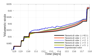
Figure 10: Volumetric strain curves for different functional dependences of $E_{sh}$ on $S_{h}$ (i.e. $c=1,2,3,5$ ) for the depressurization and gas production period.
note: ’+’ value indicates compression.

Table 1: Summary of the mathematical model

Governing equations		eqn. no.
Mass balance for each mobile component $\kappa=CH_{4},H_{2}O$	$\sum\limits_{\alpha}\left[\partial_{t}\left(\phi\ \rho_{\alpha}\ \chi_{\alpha}^{\kappa}\ S_{\alpha}\right)\right]\ +\ \sum\limits_{\alpha}\left[\nabla\cdot\left(\phi\ \rho_{\alpha}\ \chi_{\alpha}^{\kappa}\ S_{\alpha}\ {\mathbf{v}_{\alpha,t}}\right)\right]=\sum\limits_{\alpha}\left[\nabla\cdot\left(\phi\ S_{\alpha}\ {\bf J}_{\alpha}^{\kappa}\right)\right]\ +\ \dot{g}^{\kappa}\ +\ \sum\limits_{\alpha}\dot{q}_{m_{\alpha}}^{\kappa}\ +\ \dot{S}_{ext}^{\kappa}$	(1),(2)
Mass balance for hydrate phase	$\partial_{t}\left(\phi\ \rho_{h}\ S_{h}\right)\ +\ \nabla\cdot\left(\phi\ \rho_{h}\ S_{h}\ {\mathbf{v}_{h,t}}\right)\ =\ \dot{g}^{h}$	(3)
Mass balance for sand phase	$\partial_{t}\left[(1-\phi)\ \rho_{s}\right]\ +\ \nabla\cdot\left((1-\phi)\ \rho_{s}\ {\mathbf{v}_{s}}\right)\ =\ 0$	(4)
Momentum balance for mobile phases $\alpha=g,w$	${\bf v}_{\alpha}=-K\ \frac{k_{r\alpha}}{\mu_{\alpha}}\left(\nabla P_{\alpha}-\rho_{\alpha}\ {\bf g}\right)$  (Darcy’s Law)	(5),(6)
Momentum balance for	$\nabla\cdot\tilde{\sigma}+\rho_{m}\ {\bf g}=0$	(7)
composite - solid	where, $\rho_{m}$ is the bulk density given by $\ \rho_{m}=\sum\limits_{\beta}\left(\phi\ S_{\beta}\ \rho_{\beta}\right)+\left(1-\phi\right)\rho_{s}$
Energy balance	$\partial_{t}\left[\left(1-\phi\right)\rho_{s}u_{s}+\sum_{\beta}\left(\phi\ S_{\beta}\ \rho_{\beta}\ u_{\beta}\right)\right]\ +\ \sum_{\alpha}\left[\nabla\cdot\left(\phi\ \rho_{\alpha}\ \chi_{\alpha}^{\kappa}\ S_{\alpha}\ {\bf v}_{\alpha,t}\ h_{\alpha}\right)\right]\ =\ \nabla\cdot k^{c}_{eff}\nabla T\ +\ \dot{Q}_{h}\ +\ \sum\limits_{\alpha}\left(\dot{q}_{m_{\alpha}}^{\kappa}\ h_{\alpha}\right)$	(8)
	where,
	$k^{c}_{eff}=\left(1-\phi\right)k^{c}_{s}+\sum_{\alpha}\sum_{\kappa}\left(\phi\ \chi_{\alpha}^{\kappa}\ S_{\alpha}\ k_{\alpha}^{c}\right)+\phi\ S_{h}\ k_{h}^{c}$
	$h_{\alpha}=\int_{T_{ref}}^{T}Cp_{\alpha}\ dT$
	$u_{\gamma}=\int_{T_{ref}}^{T}Cv_{\gamma}\ dT$
Closure relationships
Relationship between phase pressures	$P_{g}-P_{w}=P_{c}\left(S_{we}\right)$	(9)
Summation relationships	$\sum\limits_{\beta}S_{\beta}=1$	(10)
	$\forall\alpha$ : $\sum\limits_{\kappa}\chi_{\alpha}^{\kappa}=1$	(11),(12)
Constitutive relationships
1. Vapor-liquid equilibrium
Using Henry’s Law and Raoult’s Law for ideal gas - liquid solutions,
For dissolved methane:  $\ \chi_{w}^{CH_{4}}=H(T)\ \chi_{g}^{CH_{4}}\ P_{g}$
For water vapor:     $\chi_{g}^{H_{2}O}=\chi_{w}^{H_{2}O}\ \frac{P^{sat}_{H_{2}O}(T)}{P_{g}}$
where, $H(T)$ is the Henry’s constant for methane dissolved in water calculated using the empirical relation from NIST database ([61]) , and $P^{sat}_{H_{2}O}$ is saturated water vapour pressure calculated using Antoine’s equation.
2. Diffusive mass-transfer flux
Fick’s law:	${\bf J}_{\alpha}^{\kappa}=-\tau D^{\alpha}\left(\rho_{\alpha}\nabla\chi_{\alpha}^{\kappa}\right)$
	where, $D^{\alpha}$ is the binary diffusion coefficient. $D^{g}$ is estimated using the empirical relationship proposed by [65] for low density binary $CH_{4}-H_{2}O$ system. $D^{w}$ is estimated using the Wilke-Chang correlation ([24]) for dilute associated liquid mixtures is used.
3. Hydrate phase change kinetics
Non-equilibrium phase change of methane hydrate is modeled by the Kim-Bishnoi kinetic model ([30]).
Gas generation rate     $\dot{g}^{CH_{4}}=k_{reac}\ M_{CH4}\ A_{rs}\ \left(P_{e}-f_{g}\right)$		(13)
	where, $k_{reac}$ is the rate of kinetic phase-change, $P_{e}$ is the hydrate equilibrium pressure, modelled as ([29]),
	$P_{e}=A_{1}\ \exp\left(A_{2}-\frac{A_{3}}{T}\right)$ ,	(14)
	$f_{g}$ is the gas fugacity calculated using the Peng-Robinson EoS for methane gas, and, $A_{rs}$ is the specific reaction surface area modelled as $A_{rs}=\Gamma_{r}A_{s}$, where, $A_{s}$ is the total surface area and $\Gamma_{r}$ is the ratio of the active reaction surface to the total surface area. $A_{s}$ and $\Gamma_{r}$ are modelled using the correlations proposed by [79] and [67], respectively.
Water generation rate    $\dot{g}^{H_{2}O}=\dot{g}^{CH_{4}}\ N_{Hyd}\ \frac{M_{H_{2}O}}{M_{CH_{4}}}$		(15)
Hydrate consumption rate  $-\dot{g}^{Hyd}=\dot{g}^{CH_{4}}\ \frac{M_{Hyd}}{M_{CH_{4}}}$		(16)
Heat of hydrate dissociation  $\dot{Q}_{h}=\frac{-\dot{g}^{Hyd}}{M_{Hyd}}\left(B_{1}-\frac{B_{2}}{T}\right)$		(17)
4. Properties of the fluid-matrix interaction
Capillary pressure	$P_{c}=P_{c0}\cdot f^{Pc}_{S_{h}}\left(S_{h}\right)\cdot f^{Pc}_{\phi}\left(\phi\right)$	(18)
	where, $P_{c0}$ is capillary pressure for un-deformed, un-hydrated solid matrix, given by Brooks-Corey relationship,
	$P_{c0}=P_{entry}\ S_{we}^{\ -1/\lambda_{BC}}$ ,	(19)
	and, $f^{Pc}_{S_{h}}\left(S_{h}\right)$ and $f^{Pc}_{\phi}\left(\phi\right)$ are scaling factors to account for the effects of $S_{h}$ ([57]) and $\phi$ (Civan’s power-law correlation [11]) respectively,
	$f^{Pc}_{S_{h}}=\left(1-S_{h}\right)^{-\frac{3\lambda_{BC}-1}{3\lambda_{BC}}}$  and, $\ f^{Pc}_{\phi}=\frac{\phi_{0}}{\phi}\left(\frac{1-\phi}{1-\phi_{0}}\right)^{2}$	(20)
Intrinsic permeability	$K=K_{0}\cdot f^{K}_{S_{h}}\left(S_{h}\right)\cdot f^{K}_{\phi}\left(\phi\right)$	(21)
	where, $K_{0}$ is intrinsic permeability of the un-deformed, un-hydrated solid matrix, and, $f^{K}_{S_{h}}\left(S_{h}\right)$ and $f^{K}_{\phi}\left(\phi\right)$ are scaling factors to account for the effects of $S_{h}$ ([57]) and $\phi$ ([11]) respectively,
	$f^{K}_{S_{h}}=\left(1-S_{h}\right)^{\frac{19}{6}}$  and, $\ f^{K}_{\phi}=\frac{\phi}{\phi_{0}}\left(f^{Pc}_{\phi}\right)^{-2}$	(22)
Relative permeabilities	Relative permeabilities of the mobile phases are modelled using Brooks-Corey model in conjunction with the Burdine theorem ([7]), as
	$k_{rw}=S_{we}^{\frac{2+3\lambda_{BC}}{\lambda_{BC}}}$  and, $k_{rg}=\left(1-S_{we}\right)^{2}\left(1-S_{we}^{\frac{2+\lambda_{BC}}{\lambda_{BC}}}\right)$ where, $S_{we}=\frac{S_{w}}{1-S_{h}}$	(23)
Hydraulic tortuosity	$\tau=\phi^{n}\quad$ where, $1\leq n\leq 3$	(24)
5. Poro-elasticity
Effective stress principle	Effective stress concept introduced by [70] and modified by [4] is used.
	$\tilde{\sigma}=\tilde{\sigma}^{\prime}+\alpha_{biot}\left(\frac{S_{g}P_{g}+S_{w}P_{w}}{S_{g}+S_{w}}\right)\tilde{I}$	(25)
	where, $\tilde{\sigma}$ is the total stress acting on the bulk porous medium, and $\tilde{\sigma}^{\prime}$ is the effective stress acting on the composite skeleton.
	$\alpha_{biot}$ is the Biot-Willis constant ([5]).
Linear elastic law	$\tilde{\sigma}^{\prime}=2\ G_{sh}\ \tilde{\epsilon}+\lambda_{sh}(tr\ \tilde{\epsilon})\ \tilde{I}$	(26)
	where, $\tilde{\epsilon}$ is the linearized strain, given by $\quad\tilde{\epsilon}=\frac{1}{2}\left(\nabla{\bf u}+\nabla^{T}{\bf u}\right)$	(27)
	and, $G_{sh}$ and $\lambda_{sh}$ are the Lame’s parameters.
Young’s modulus	Young’s modulus $E_{sh}$ is modelled using the parameterization proposed by [62]: $E_{sh}=E_{s}+S_{h}^{c}\ E_{h}$
	where, $E_{s}$ and $E_{h}$ are the Young’s modulus of hydrate-free sand and hydrate, respectively.	(28)

Table 2: Material properties and model parameters

Thermal conductivities				Ref.
$k^{c}_{g}$	$-0.886\times 10^{-2}+0.242\times 10^{-3}T-0.699\times 10^{-6}T^{2}+0.122\times 10^{-8}T^{3}$		$W\cdot m^{-1}\cdot K^{-1}$	[58]
$k^{c}_{w}$	$0.3834\ ln(T)-1.581$		$W\cdot m^{-1}\cdot K^{-1}$	[74]
$k^{c}_{h}$	$2.1$		$W\cdot m^{-1}\cdot K^{-1}$	[64]
$k^{c}_{s}$	$1.9$		$W\cdot m^{-1}\cdot K^{-1}$	[17]
Specific heat capacities
$Cp_{g}$	$\Delta Cp^{res}_{g}\left(1238+3.13T+7.9\times 10^{-4}T^{2}\right.$
	$\left.-6.86\times 10^{-7}T^{3}\right)$		$J\cdot kg^{-1}\cdot K^{-1}$	[54, 17]
$Cv_{g}$	$Cp_{g}+R_{CH_{4}}$		$J\cdot kg^{-1}\cdot K^{-1}$
$Cp_{w}$	$4186$		$J\cdot kg^{-1}\cdot K^{-1}$	[74]
$Cv_{w}$	$Cp_{w}+R_{H_{2}O}$		$J\cdot kg^{-1}\cdot K^{-1}$
$Cv_{h}$	$2700$		$J\cdot kg^{-1}\cdot K^{-1}$	[64]
$Cv_{s}$	$800$		$J\cdot kg^{-1}\cdot K^{-1}$	[17]
Dynamic viscosities
$\mu_{g}$	$10.4\times 10^{-6}\left(\frac{273.15+162}{T+162}\right)\left(\frac{T}{273.15}\right)^{1.5}$		$Pa\cdot s$	[18]
$\mu_{w}$	$0.001792\ \exp\left[-1.94-4.80\left(\frac{273.15}{T}\right)\right.$
	$\left.+6.74\left(\frac{273.15}{T}\right)^{2}\right]$		$Pa\cdot s$	[74]
Densities
$\rho_{g}$	$\frac{P_{g}}{zR_{g}T}$		$kg\cdot m^{-3}$	[54]
$\rho_{w}$	vapour:	$0.0022\frac{P_{g}}{T}$	$kg\cdot m^{-3}$	[74]
	liquid:	$1000$	$kg\cdot m^{-3}$	[74]
$\rho_{h}$	$900$		$kg\cdot m^{-3}$	[64]
$\rho_{s}$	$2100$		$kg\cdot m^{-3}$
Hydraulic properties
$\lambda_{BC}$	$1.2$			[23]
$P_{entry}$	$50$		$kPa$	[23]
Hydrate kinetics
$k_{reac}$	formation:	$0.2\times 10^{-11}$	mol$\cdot m^{-2}\cdot$
	dissociation:	$3.2\times 10^{-10}$	$Pa^{-1}\cdot s^{-1}$
$N_{Hyd}$	$5.75$
$P_{e,0}$	$A_{1}=10^{6}$, $A_{2}=38.98$, $A_{3}=8533.8$		$Pa$	[28]
$\dot{Q}_{h}$	$B_{1}=56599$, $B_{2}=16.744$		$W\cdot m^{-3}$	[17]
Poroelasticity parameters
$\alpha_{biot}$	$0.8$			[73]
$\nu_{sh}$	$0.15$			[45]
	formation	dissociation
$E_{s}$	$32$	$160$	$MPa$
$E_{h}$	$250$	$360$	$MPa$
$c$	$1$	$3$

Acknowledgements

We gratefully acknowledge the support for the first author by the German Research Foundation (DFG), through project no. WO 671/11-1. This work was further funded by the German Federal Ministries of Economy (BMWi) and Education and Research (BMBF) through the SUGAR project (grant No. 03SX250, 03SX320A & 03G0856A), and the EU-FP7 project MIDAS (grant agreement no. 603418). The reported experimental data is attached as supplemental material with this article.

References

- [1] G. Ahmadi, C. Ji, and H.S. Duane. Numerical solution for natural gas production from methane hydrate dissociation. J. Pet. Sci. Eng., 41:169–185, 2004.
- [2] B. Anderson, R. Boswell, Collett T.S., H. Farrell, S. Ohtsuki, M. White, and M. Zyrianova. Review of the findings of the ignik sikumi co2-ch4 gas hydrate exchange field trial. In Proceedings of the 8th International Conference on Gas Hydrates, Beijing, China, 2014. ICGH8.
- [3] D. Archer, B. Buffett, and V. Brovkin. Ocean methane hydrates as a slow tipping point in the global carbon cycle. Proc. Nat. Acad. Sci. USA, 106:20596–20601, 2009.
- [4] M.A. Biot. General theory of three-dimensional consolidation. J. Appl. Phys., 12:155–164, 1941.
- [5] M.A. Biot and D.G. Willis. The elastic coefficients of the theory of consolidation. J. Appl. Mech., 24:594–601, 1957.
- [6] J. Brugada, Y.P. Cheng, K. Soga, and J.C. Santamarina. Discrete element modelling of geomechanical behaviour of methane hydrate soils with pore-filling hydrate distribution. Granular Matter, 12(5):517–525, 2010.
- [7] N.T. Burdine. Relative permeability calculations from pore-size distribution data, technical report. Technical report, Petroleum Transanctions, AIME, 1953.
- [8] E.B. Burwicz, L.H. Rüpke, and K. Wallmann. Estimation of the global amount of submarine gas hydrates formed via microbial methane formation based on numerical reaction-transport modeling and a novel parameterization of holocene sedimentation. Geochim. Cosmochim. Acta, 75:4562–4576, 2011.
- [9] J.H. Choi, S. Dai, J.H. Cha, and Y. Seol. Laboratory formation of noncementing hydrates in sandy sediments. Geochemistry, Geophysics, Geosystems, 15(4):1648–1656, 2014.
- [10] Z.R. Chong, M. Yang, B.C. Khoo, and P. Linga. Size effect of porous media on methane hydrate formation and dissociation in an excess gas environment. Industrial and Engineering Chemistry Research, 55(29):7981–7991, 2016.
- [11] F. Civan. Predictability of porosity and permeability alterations by geochemical and geomechanical rock and fluid interactions. In SPE 58746, 2000.
- [12] C. David. Japanese test coaxes fire from ice. Nature, 496, 409 (April 25, 2013), 2013.
- [13] A. Dedner, B. Flemisch, and R. Klöfkorn. Advances in DUNE: Proceedings of the DUNE User Meeting, Held in October 6th–8th 2010 in Stuttgart, Germany. SpringerLink : Bücher. Springer Berlin Heidelberg, 2012.
- [14] J.W. Demmel, J.R. Gilbert, and X.S. Li. Superlu users’ guide. Technical Report LBNL-44289, Lawrence Berkeley National Laboratory, 1999. Last update: September 2007.
- [15] C. Deusner, S. Gupta, E. Kossel, M. Freise, H. Anbergen, T. Wille, N. Bigalke, and M. Haeckel. The role of high-pressure flow-through experiments for evaluating the mechanical behaviour of gas hydrate-bearing soils. In F. Wuttke, S. Bauer, and M. Sanchez, editors, Energy Geotechnics. CRC Press.
- [16] Christian Deusner, Nikolaus Bigalke, Elke Kossel, and Matthias Haeckel. Methane production from gas hydrate deposits through injection of supercritical co2. Energies, 5(7):2112, 2012.
- [17] F. Esmaeilzadeh, M. E. Zeighami, and J. Fathi. 1-d modeling of hydrate decomposition in porous media. International Journal of Chemical, Molecular, Nuclear, Materials and Metallurgical Engineering, 2(5):45–51, 2008.
- [18] Daniel G. Friend, James F. Ely, and Hepburn Ingham. Thermophysical properties of methane. Journal of Physical and Chemical Reference Data, 18(2):583–638, 1989.
- [19] S. Gupta, B. Wohlmuth, and R. Helmig. Multi-rate time stepping schemes for hydro-geomechanical model for subsurface methane hydrate reservoirs. Preprint in Advances in water resources, 2016.
- [20] Shubhangi Gupta, Rainer Helmig, and Barbara Wohlmuth. Non-isothermal, multi-phase, multi-component flows through deformable methane hydrate reservoirs. Computational Geosciences, pages 1–26, 2015.
- [21] C. Hager and B. Wohlmuth. Semismooth newton methods for variational problems with inequality constraints. GAMM Mitteilungen, 33:8–24, 2010.
- [22] Corinna Hager and B.I. Wohlmuth. Nonlinear complementarity functions for plasticity problems with frictional contact. Computer Methods in Applied Mechanics and Engineering, 198(41):3411 – 3427, 2009.
- [23] R. Helmig. Multiphase Flow and Transport Processes in the Subsurface: A Contribution to the Modeling of Hydrosystems, volume 91. Springer-Verlag, Berlin, 2016.
- [24] D. M. Himmelblau. Diffusion of dissolved gases in liquids. Chem. Rev., 64(5):527–550, 1964.
- [25] M. Hyodo, Y. Li, J. Yoneda, Y. Nakata, N. Yoshimoto, and A. Nishimura. Effects of dissociation on the shear strength and deformation behavior of methane hydrate-bearing sediments. Marine and Petroleum Geology, 51:52 – 62, 2014.
- [26] G. Janicki, S. Schlüter, To. Hennig, H. Lyko, and G. Deerberg. Simulation of methane recovery from gas hydrates combined with storing carbon dioxide as hydrates. Journal of Geological Research, 2011, Article ID 462156:1–15, 2011.
- [27] Y. Jin, Y. Konno, and J. Nagao. Growth of methane clathrate hydrates in porous media. Energy and Fuels, 26(4):2242–2247, 2012.
- [28] V. A. Kamath and G. D. Holder. Dissociation heat transfer characteristics of methane hydrates. AIChe J., 33:347–350, 1987.
- [29] V.A. Kamath. Study of heat transfer characteristics during dissociation of gas hydrates in porous media. PhD thesis, Univ. of Pittsburgh,Pittsburgh, PA, Jan 1984.
- [30] H.C. Kim, P.R. Bishnoi, R.A. Heidemann, and S.S.H. Rizvi. Kinetics of methane hydrate decomposition. Chemical Engineering Science, 42(7):1645–1653, 1987.
- [31] S. Kimoto, F. Oka, and T. Fushita. A chemo-thermo-mechanically coupled analysis of ground deformation induced by gas hydrate dissociation. International Journal of Mechanical Sciences, 52(2):365–376, 2010.
- [32] A. Klar, K. Soga, and Y.A. NG. Coupled deformation-flow analysis for methane hydrate extraction. Geotechnique, 60(10):765–776, 2010.
- [33] A. Klar, S. Uchida, K. Soga, and K. Yamamoto. Explicitly coupled thermal flow mechanical formulation for gas-hydrate sediments. SPE J., 18:196–206, 2013.
- [34] M. Kurihara, A. Sato, H. Ouchi, H. Narita, Y. Masuda, T. Saeki, and T. Fujii. Prediction of gas productivity from eastern nankai trough methane-hydrate reservoirs. SPE125481, SPE Reservoir Eval. Eng., 12:477–499, 2009.
- [35] K.A. Kvenvolden. Gas hydrates, geological perspective and global change. Rev. Geophys., 31:173–187, 1993.
- [36] H. Lee, Y. Seo, Y.-T. Seo, I.L. Moudrakovski, and J.A. Ripmeester. Recovering methane from solid methane hydrate with carbon dioxide. Angew. Chem. Int. Ed., 42:5048–5051, 2003.
- [37] J. Y. Lee, J. Carlos Santamarina, and C. Ruppel. Volume change associated with formation and dissociation of hydrate in sediment. Geochemistry, Geophysics, Geosystems, 11(3), 2010. Q03007.
- [38] J.Y. Lee, F.M. Francisca, J.C. Santamarina, and C. Ruppel. Parametric study of the physical properties of hydrate-bearing sand, silt, and clay sediments: 2. small-strain mechanical properties. Journal of Geophysical Research, 115(B11):11p, 2010.
- [39] Jeen-Shang Lin, Yongkoo Seol, and Jeong Hoon Choi. An smp critical state model for methane hydrate-bearing sands. International Journal for Numerical and Analytical Methods in Geomechanics, 39(9):969–987, 2015. NAG-14-0044.R1.
- [40] X. Liu and P.B. Flemings. Dynamic multiphase flow model of hydrate formation in marine sediments. J. Geophys. Res., 112, 2007.
- [41] Alexander Mielke. Existence of minimizers in incremental elasto-plasticity with finite strains. SIAM J. Math. Anal., 36(2):384–404, 2004.
- [42] Alexander Mielke. Global existence for rate-independent gradient plasticity at finite strain. J. Nonlinear Sci., 19(3):221–248, 2009.
- [43] Alexei V. Milkov. Global estimates of hydrate-bound gas in marine sediments: how much is really out there? Earth-Science Reviews, 66(3-4):183–197, 2004.
- [44] K. Miyazaki, A. Masui, K. Aoki, Y. Sakamoto, T. Yamaguchi, and S. Okubo. Strain-rate dependence of triaxial compressive strength of artificial methane-hydrate-bearing sediment. International Journal of Offshore and Polar Engineering, 20(4):256–264, 2010.
- [45] K. Miyazaki, A. Masui, Y. Sakamoto, K. Aoki, N. Tenma, and T. Yamaguchi. Triaxial compressive properties of artificial methane-hydrate-bearing sediment. J. Geophys. Res.-Solid Earth, 116:B06102, 2011.
- [46] Kuniyuki Miyazaki, Kazuo Aoki, Norio Tenma, Yasuhide Sakamoto, Tsutomu Yamaguchi, et al. Application of nonlinear elastic constitutive model to analysis of artificial methane-hydrate-bearing sediment sample. In Ninth ISOPE Ocean Mining Symposium. International Society of Offshore and Polar Engineers, 2011.
- [47] Kuniyuki Miyazaki, Norio Tenma, Kazuo Aoki, and Tsutomu Yamaguchi. A nonlinear elastic model for triaxial compressive properties of artificial methane-hydrate-bearing sediment samples. Energies, 5(10):4057–4075, 2012.
- [48] G.J. Moridis. Numerical studies of gas production from methane hydrates. SPE 87330, SPE J., 32(8):359–370, 2003.
- [49] G.J. Moridis, T.S. Collett, R. Boswell, M. Kurihara, M.T. Reagan, C. Koh, and E.D. Sloan. Toward production from gas hydrates: Current status, assessment of resources, and simulation-based evaluation of technology and potential. SPE Reserv. Eval. Eng., 12:745–771, 2009.
- [50] G.J. Moridis, T.S. Collett, M. Pooladi-Darvish, S. Hancock, C. Santamarina, R. Boswell, T. Kneafsey, J. Rutqvist, M.B. Kowalsky, and et al. Reagan, M.T. Challenges, uncertainities and issues facing gas production from gas hydrate deposits. SPE Reserv. Eval. Eng., 14:76–112, 2011.
- [51] G.J. Moridis, M. Kowalsky, and K. Pruess. Depressurization-inducedgas production from class-i hydrate deposits. SPE J. Reservoir Evaluation Engng, 10(5):458–481, 2007.
- [52] G.J. Moridis, M.B. Kowalsky, and K. Pruess. TOUGH-Fx/HYDRATE v1.0 User’s manual: A code for the simulation of system behaviour in hydrate-bearing geologic media. Earth Sciences Division, Lawrence Berkeley National Laboratory, Berkeley, California, 2008.
- [53] Y. Park, D.-Y. Kim, J.-W. Lee, D.-G. Huh, K.-P. Park, J. Lee, and H. Lee. Sequestering carbon dioxide into complex structures of naturally occurring gas hydrates. Proc. Nat. Acad. Sci. USA, 103:12690–12694, 2006.
- [54] D. Y. Peng and D. B. Robinson. A new two-constant equation of state. Industrial and Engineering Chemistry: Fundamentals, 15:59–64, 1976.
- [55] E. Piñero, M. Marquardt, C. Hensen, M. Haeckel, and K. Wallmann. Estimation of the global inventory of methane hydrates in marine sediments using transfer functions. Biogeosciences, 10(2):959–975, 2013.
- [56] Jeffrey A. Priest, Emily V. L. Rees, and Christopher R. I. Clayton. Influence of gas hydrate morphology on the seismic velocities of sands. Journal of Geophysical Research: Solid Earth, 114(B11), 2009. B11205.
- [57] M.L. Rockhold, R.R. Yarwood, M.R. Niemet, P.J. Bottomley, and J.S. Selker. Considerations for modelling bacterial-induced changes in hydraulic properties of variably sarurated porous media. Advances in Water Resources, 25:477–495, 2002.
- [58] H.M. Roder. Thermal conductivity of methane for temperatures between 110 k and 310 k with pressures upto 70 mpa. Journal of Thermophysics, 6(2):119–142, 1985.
- [59] J. Rutqvist. Status of the tough-flac simulator and recent applications related to coupled fluid flow and crustal deformations. Computers & Geosciences, 37:739–750, 2011.
- [60] J. Rutqvist, G.J. Moridis, T. Grover, and Collett T. Geomechanical response of permafrost-associated hydrate deposits to depressurization-induced gas production. Journal of petroleum science and engineering, 67(1-2):1–12, 2009.
- [61] R. Sander. Henry’s law constants. In P.J. Linstrom and W.G. Mallard, editors, NIST Chemistry WebBook, number 69 in NIST Standard Reference Database. National Institute of Standards and Technology, Gaithersburg MD, 20899, retrieved February 23, 2015.
- [62] J. C. Santamarina and C. Ruppel. The impact of hydrate saturation on the mechanical, electrical, and thermal properties of hydrate-bearing sand, silts, and clay in geophysical characterization of gas hydrates. Geo-phys. Dev. Ser., edited by M. Riedel, C. Willoughby, and S. Chopra, Soc. of Explor. Geophys., Tulsa, Okla, 14:373–384, 2010.
- [63] D. Schoderbek, H. Farrell, K. Hester, J. Howard, K. Raterman, S. Silpngarmlert, K.L. Martin, B. Smith, and P. Klein. Conocophillips gas hydrate production test final technical report. Technical report, ConocoPhillips, 2013.
- [64] E.D. Sloan and C. Koh. Clathrate Hydrates of Natural Gases, Third Edition. Chemical Industries. CRC Press, 2007.
- [65] J.C. Stattery and R.B. Bird. Calculation of diffusion coefficient of dilute gases and of the self diffusion coefficient of dense gases. AIChE J., 4(2):137–142, 1958.
- [66] L A Stern, S Circone, S H Kirby, and W B Durham. Temperature, pressure, and compositional effects on anomalous or ”self” preservation of gas hydrates. Canadian Journal of Physics, 81(1-2):271–283, 2003.
- [67] F.X. Sun and K.K. Mohanty. Kinetic simulation of methane hydrate formation and dissociation in porous media. Chemical Engineering Science, 61:3476–3495, 2006.
- [68] F.X. Sun, K.K. Mohanty, and N. Nanchary. 1-d modelling of hydrate depressurization in porous media. Transp. Porous Med., 58:315–338, 2005.
- [69] Xiang Sun, Xiaoxia Guo, Longtan Shao, and Hongxiang Tang. A thermodynamics-based critical state constitutive model for methane hydrate bearing sediment. Journal of Natural Gas Science and Engineering, 27, Part 2:1024 – 1034, 2015.
- [70] K. Terzaghi. Erdbaumechanik auf bodenphysikalischer Grundlage. F. Deuticke, Wien, 1925.
- [71] G.G. Tsypkin. Effect of liquid phase mobility on gas hydrate dissociation in reservoirs. Izvestiya Akad. Nauk SSSR. Mekh. Zhidkosti i Gaza., 4:105–114, 1991.
- [72] S. Uchida, K. Soga, and K. Yamamoto. Critical state soil constitutive model for methane hydrate soil. Journal of Geophysical Research: Solid Earth, 117(B3):n/a–n/a, 2012. B03209.
- [73] A. Verruijt. Encyclopedia of Hydrological Sciences, chapter Consolidation of soils. Wiley, Chichester, UK, 2008.
- [74] Wolfgang Wagner and Hans-Joachim Kretzschmar. Iapws industrial formulation 1997 for the thermodynamic properties of water and steam. International Steam Tables: Properties of Water and Steam Based on the Industrial Formulation IAPWS-IF97, pages 7–150, 2008.
- [75] W. F. Waite, J. C. Santamarina, D. D. Cortes, B. Dugan, D. N. Espinoza, J. Germaine, J. Jang, J. W. Jung, T. J. Kneafsey, H. Shin, K. Soga, W. J. Winters, and T. S. Yun. Physical properties of hydrate-bearing sediments. Reviews of Geophysics, 47(4), 2009.
- [76] M.D. White and B.P. McGrail. Stomp-hyd: A new numerical simulator for analysis of methane hydrate production from geologic formations. In JJ Bahk A Reedman, YS Park and N Chaimanee, editors, Proceedings of 2nd International Symposium on Gas Hydrate Technology, pages 77–86. CCOP, 2006.
- [77] K. Yamamoto. Japan completes first offshore methane hydrate production test - methane successfully produced from deepwater hydrate layers. fire in the ice: Department of energy, office of fossil energy, national energy technology laboratory. Methane Hydrate News Letter, 13(1-2), 2013.
- [78] K. Yamamoto. Overview and introduction: pressure core-sampling and analyses in the 2012-2013 mh21 offshore test of gas production from methane hydrates in the eastern nankai trough. Marine and Petroleum Geology, 2015.
- [79] M.H. Yousif. Experimental and theoretical investigation of methane-gas-hydrate dissociation in porous media. SPE Reserv. Eng., pages 69–76, 1991.
- [80] Feng Yu, Yongchen Song, Weiguo Liu, Yanghui Li, and Weihaur Lam. Analyses of stress strain behavior and constitutive model of artificial methane hydrate. Journal of Petroleum Science and Engineering, 77(2):183 – 188, 2011.
- [81] T.S. Yun, J.C. Santamarina, and C. Ruppel. Mechanical properties of sand, silt, and clay containing tetrahydrofuran hydrate. J. Geophys. Res., 112:B04106, 2007.