Accelerating the convergence of replica exchange simulations
using Gibbs sampling and adaptive temperature sets

Abstract

We recently introduced a novel replica-exchange scheme in which an individual replica can sample from states encountered by other replicas at any previous time by way of a global configuration database, enabling the fast propagation of relevant states through the whole ensemble of replicas. This mechanism depends on the knowledge of global thermodynamic functions which are measured during the simulation and not coupled to the heat bath temperatures driving the individual simulations. Therefore, this setup also allows for a continuous adaptation of the temperature set. In this paper, we will review the new scheme and demonstrate its capability. The method is particularly useful for the fast and reliable estimation of the microcanonical temperature $T(U)$ or, equivalently, of the density of states $g(U)$ over a wide range of energies.

I Introduction

Simulating physical systems exhibiting multifaceted structural transitions (encountered, for example, in many protein folding problems) or containing extremely hard to find but thermodynamically important states (e.g., crystalline states in hard materials) is a notorious challenge. Replica-exchange (RE) and multicanonical (MUCA) sampling schemes have both been applied, in conjunction with Monte Carlo (MC) and molecular dynamics (MD) methods, to address this issue. They enable the investigation of systems at multiple or varying temperatures, such facilitating the exploration of the configurational space. One of the main practical challenges in the case of RE is the determination of good temperature sets for the heat baths. To this day, many sophisticated schemes have been proposed to solve this problem, see, e.g., Rathore et al. (2005); Katzgraber et al. (2006); Patriksson and van der Spoel (2008); Guidetti et al. (2012); Ballard and Wales (2014). Another limitation of generic RE schemes is that exchange of configurations obviously does not, on its own, change the ensemble of configurations present in the simulation. This is not optimal if the simulation is not converged yet, e.g., if some replicas have yet to locate all thermodynamically relevant states. In this case, some sort of population control, where “good” configurations can be multiplied and “irrelevant” ones deleted, can help (see Hsu and Grassberger (2011) for an example).

MUCA simulations offer a different strategy to efficiently sample configuration space. In the case of MD, MUCA sampling simply consists of rescaling the interatomic forces: $f_{\mathrm{muca}}=(T_{0}/T(U))\,f_{\mathrm{can}}$ Hansmann et al. (1996); Junghans et al. (2014), where $f_{\mathrm{can}}=-\nabla U$ are the conventional forces and $T(U)$ is the microcanonical temperature. The difficulty lies in the estimation of this a priori unknown function. Metadynamics Laio and Parrinello (2002); Dama et al. (2014) and statistical temperature molecular dynamics (STMD) Kim et al. (2006) were successfully applied to this problem. However, these methods can show dynamical artifacts like hysteresis when the system is driven over first-order like transitions, for example. Further, even with the knowledge of $T(U)$, the diffusion of a MUCA simulation in energy space can be very slow. However, a very powerful side-effect of MUCA simulations is that, once obtained, $T(U)$ can be used to infer the density of states, hence providing a wealth of thermodynamic information.

In the following, we review a generalized RE method, the Gibbs-sampling enhanced RE, which addresses some of the issues with generic RE and MUCA simulations. By uncoupling the measured microcanonical temperature from the heat-bath temperatures which drive the simulations we can introduce powerful conformational mixing steps and continuously adapt the heat-bath temperatures for a complete coverage of the whole energy range. We demonstrate this ability by presenting a particular adaptive simulation which is set up so that only a tiny part of the phase space in covered the beginning. Note that $T(U)$ is also available at the end of such a simulation, providing an alternative to conventional MUCA approaches.

II Method review

We consider a RE scheme Geyer (1991) in an expanded-canonical ensemble Lyubartsev et al. (1992) with reference temperatures $T_{0}^{i}$. In contrast to other sampling methods where thermodynamic functions are continuously adapted Wang and Landau (2001); Laio and Parrinello (2002); Junghans et al. (2014), the basic idea in our method Vogel and Perez (2015) is to measure the microcanonical temperature while running canonical simulations, hence decoupling the measurements from the simulation-driving heat bath temperatures. We use an estimator for the microcanonical temperature based the microcanonical averages of time-derivatives of the product between the normalized energy gradient $\eta=\nabla U/(\nabla U\nabla U)$ and the particle momenta $p$:

$$g=\frac{\mathrm{d}F(U)}{\mathrm{d}U}=-\left\langle\frac{\mathrm{d}}{\mathrm{d}t}(\eta\cdot p)\right\rangle\,,$$ (1)

where $F$ is the free energy, a relation which was derived in a more general form in the context of the adaptive biasing force (ABF) method Darve et al. (2008). The time derivatives are estimated in an additional, constant-energy MD time step. As defined, $g$ relates to the microcanonical temperature as:

$$T_{\mathrm{ABF}}(U)=\frac{T_{0}}{1-g}\,.$$ (2)

During the simulation, all replicas contribute measurements to the global calculation of $T_{\mathrm{ABF}}(U)$, while they also collectively fill a global conformational database. An instantaneous estimator for the (unnormalized) entropy $S(U)$ can then be obtained:

$$S(U)=\int_{U_{0}}^{U}T^{-1}_{\mathrm{ABF}}(U^{\prime})\,\mathrm{d}U^{\prime}+C\,.$$ (3)

With $g(U)=\mathrm{exp}[k_{B}^{-1}S(U)]$ being the density of states, canonical energy probability distributions $P_{i}(U)\propto g(U)\,\mathrm{e}^{-\beta_{i}U}$ can be calculated. The key is that these distributions calculated from global data are different from those that would be inferred from the data gathered by individual walkers alone. For example, $P_{i}(U)$ can account for the presence of some low energy state, even though walker $i$ might never have sampled it himself. This allows for the introduction of a rejection-free, global Monte Carlo move facilitating the propagation of important states through the simulation: at any time, a walker can sample a new energy value from the distribution $P_{i}(U)$ (a so-called “Gibbs sampling” move) and replace its actual configuration by one with that energy ($\pm\epsilon$, for practical reasons) from the global configuration database. Such moves allow each replica to properly sample from the pool of states visited by all other replicas.

III The adaptive temperature set

In RE, good performance relies on a proper choice of temperatures, as this determines the exchange probabilities between neighboring replicas, say $i$ and $i+1$. Assuming the corresponding canonical distributions $P_{i}(U)$ and $P_{i+1}(U)$ are known, the exchange probabilities $W_{i}(P_{i},P_{i+1})$ read:

$$W_{i}(P_{i},P_{i+1})$$

$$=\int_{-\infty}^{\infty}P_{i}(U)\int_{-\infty}^{\infty}W_{\mathrm{acc}}(U,U^{\prime})P_{i+1}(U^{\prime})\,\mathrm{d}U\mathrm{d}U^{\prime}\,,$$ (4)

with

$$W_{\mathrm{acc}}(U,U^{\prime})=\min\left\{1,\mathrm{exp}\left[(\beta_{i+1}-\beta_{i})(U^{\prime}-U)\right]\right\}$$ (5)

being the RE acceptance probability. These $W_{i}(P_{i},P_{i+1})$ can be approximated (see Nadler and Hansmann (2007), for example), but with the knowledge of a global, instantaneous $T(U)$ and hence of $g(U)$ and $P_{i}(U)$, the $W_{i}(P_{i},P_{i+1})$ can be calculated. We can then find a temperature set $\beta^{-1}_{i}=k_{B}T_{0}^{i}$, $(i=1,\ldots,n)$, such that [cf. Nadler and Hansmann (2007); Bittner et al. (2008)]

$$W_{i}(P_{i},P_{i+1})=\mathrm{const}\quad\forall i\,.$$ (6)

Such a criterion would be optimal in the limit where sampling is ergodic on the timescale of exchange attempts Nadler and Hansmann (2007); Bittner et al. (2008). When this condition is broken, it might instead be preferable to directly minimize the tunneling time  Katzgraber et al. (2006).

Since there is no need for the reference temperatures $T_{0}^{i}$ to remain constant for the calculation of $T_{\mathrm{ABF}}(U)$ or other thermodynamic averages, these can be freely changed during the simulation. With a given, fixed number of processors, there are two options: either require a fixed value for the constant in Eq. 6 (resulting in a fluctuating total temperature range) or fix the global temperature range (and thus correspondingly adjusts the value of the constant). We chose the latter to ensure we always cover the whole temperature range and adjust the temperatures using a bisection scheme.

IV Demonstration

Figure 1: Representative configurations of the 500-silver atom system. From left to right: an amorphous state; the pure crystalline (ground-) state; two crystalline states with stacking faults.

Figure 2: Snapshots of the instantaneous estimator for the microcanonical temperature (red, solid line) at different times during the simulation. The dots correspond to raw measurements entering in the average (cf. Eqs. 1 and 2). Different colors and symbols correspond to different reference temperatures $T_{0}^{i}$. Raw measurements are only shown for every other reference temperature. Only 10% of the raw data are shown for clarity. The last plot (f) also contains data from pure RE and from STMD (see text for details).

Figure 3: (a) Measured replica-exchange acceptance rates for all neighbor pairs ($i,i+1$) over time. (b) Time evolution of the temperature set $T_{0}^{i}$.

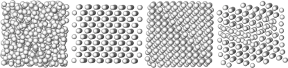
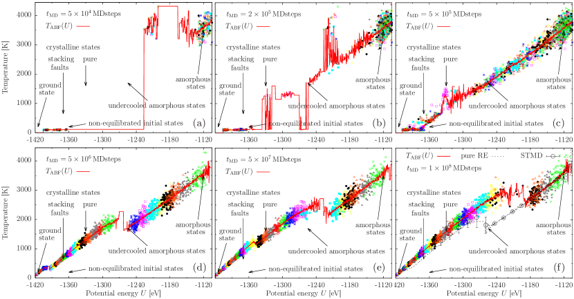
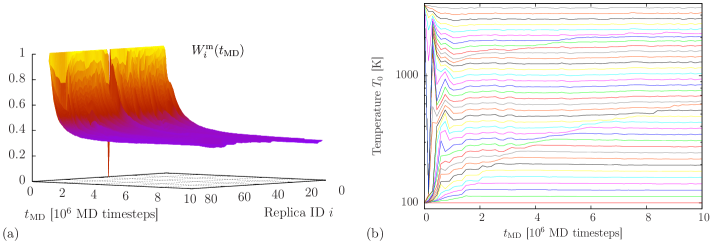
We illustrate the performance of the method for a system of 500 silver atoms interacting via an embedded atom potential Williams et al. (2006). We use a constant particle density of $\rho=0.0585\AA^{-3}$ and perform a Gibbs-sampling enhanced RE simulation based on molecular dynamics runs at heat-bath temperatures $T_{0}^{i}$. Representative configurations are shown in Fig. 1. We begin the simulation in an extremely unnatural way: of the 71 individual canonical walkers, half of them start at the minimum temperature of $T_{0}^{i<35}=T_{\mathrm{min}}=100$ K and the other half at the maximum temperature $T_{0}^{i\geq 35}=T_{\mathrm{max}}=3500$ K. Furthermore, all replicas begin from an amorphous configuration. Figure 2 shows snapshots of the instantaneous microcanonical temperature measured as $T_{\mathrm{ABF}}(U)$ (cf. Eq. 2) for different simulation times $t_{\mathrm{MD}}$. Shortly after starting the simulation (Fig. 2 a) and before the first temperature adaptation, we only find configurations with temperatures scattered around the initial values $T_{\mathrm{min}}$ and $T_{\mathrm{max}}$. The instantaneous temperature $T_{\mathrm{ABF}}(U)$ is completely arbitrary at this point. The next snapshot (b) was taken after the first temperature adaptation and the exploration of configurations at intermediate energies starts. After about $5\times 10^{5}$ MD steps (Fig. 2 c; temperature adaptation takes place every $1.5\times 10^{5}$ MD steps) temperatures are already spread out such that the whole energy range is covered. The ground state has been discovered after $5\times 10^{6}$ MD steps (d) and propagates through the simulation (e) facilitated by the Gibbs sampling moves. The simulation eventually converges after approximately $1\times 10^{8}$ MD steps (f). Note that we set a memory time after which data is discarded, so that non-equilibrated states encountered in the beginning do not enter in the averages (Eqs. 1 and 2) at later times.

We show in Fig. 3 the measured replica-exchange acceptance rate $W_{i}^{\mathrm{m}}$ (a) and the values of the heat bath temperatures $T_{0}^{i}$ (b) as the simulation time progresses. In accordance to the discussion above, $W_{i}^{\mathrm{m}}=0$ for the exchange between the two neighboring walkers at $T_{\mathrm{min}}$ and $T_{\mathrm{max}}$ and $W_{i}^{\mathrm{m}}=1$ everywhere else. After a short time, however, all measured acceptance rates approach a constant value of $W_{i}^{\mathrm{m}}\approx 0.35$. This value is in agreement with the calculated value for the constraint given in Eq. 6 for our particular set-up, i.e., for the fixed temperature range and the number of walkers we employ. Note that we can directly control the value of $W_{i}^{\mathrm{m}}$ by deploying more or less walkers. The adaptation speed of the replica-exchange rates is of course related to the adaption speed of the temperature set $T_{0}^{i}$. It can be seen in Fig. 3 b that very few temperature adaptation steps are required before they are reasonably well distributed. Adaptation is marginal at times $t_{\mathrm{MD}}\gtrsim 1\times 10^{6}$ and is mainly in response to the propagation of the ground-state, as this creates an artificial signal of a “phase transition” in $T_{\mathrm{ABF}}(U)$ and the temperatures get locally closer together around the corresponding “transition temperature”.

Finally, in Fig. 2 f, we also provide data from a pure RE exchange run (i.e., w/o Gibbs moves) at the same time and from multiple Gauss-kernel STMD Junghans et al. (2014) runs, for comparison. While the pure RE run did not converge at all after this time and mainly samples configurations with stacking faults in the crystalline phase, the STMD run samples both, pure and defected states but suffers from hysteresis. While both conventional methods are not able to converge in this challenging situation, our method including additional Gibbs-sampling moves works remarkably well.