Chimera states in coupled Kuramoto oscillators with inertia

Abstract

The dynamics of two symmetrically coupled populations of rotators is studied for different values of the inertia. The system is characterized by different types of solutions, which all coexist with the fully synchronized state. At small inertia the system is no more chaotic and one observes mainly quasi-periodic chimeras, while the usual (stationary) chimera state is not anymore observable. At large inertia one observes two different kind of chaotic solutions with broken symmetry: the intermittent chaotic chimera, characterized by a synchronized population and a population displaying a turbulent behaviour, and a second state where the two populations are both chaotic but whose dynamics adhere to two different macroscopic attractors. The intermittent chaotic chimeras are characterized by a finite life-time, whose duration increases as a power-law with the system size and the inertia value. Moreover, the chaotic population exhibits clear intermittent behavior, displaying a laminar phase where the two populations tend to synchronize, and a turbulent phase where the macroscopic motion of one population is definitely erratic. In the thermodynamic limit these states survive for infinite time and the laminar regimes tends to disappear, thus giving rise to stationary chaotic solutions with broken symmetry contrary to what observed for chaotic chimeras on a ring geometry.

In 2002, simulations of abstract mathematical models revealed the existence of counterintuitive “chimera states”, where an oscillator population splits into two parts, with one synchronizing and the other oscillating incoherently, even though the oscillators are identical. Since then, these counterintuitive states have become a relevant subject of investigation for experimental and theoretical scientists active in different fields, as testified by the rapidly increasing number of publications in recent years (for a review see Motter (2010); Panaggio and Abrams (2015)). In this paper we analyze novel chimera states emerging in two symmetrically coupled populations of oscillators with inertia. In particular, the introduction of inertia allows the oscillators to synchronize via the adaptation of their own frequencies, in analogy with the mechanism observed in the firefly Pteroptix malaccae Ermentrout (1991). The modification of the classical Kuramoto model with the addition of an inertial term results in first order synchronization transitions and complex hysteretic phenomena Tanaka et al. (1997a, b); Ji et al. (2013); Gupta et al. (2014); Komarov et al. (2014); Olmi et al. (2014). Furthermore, networks of rotators have recently found applications in different technological contexts, including disordered arrays of Josephson junctions Trees et al. (2005) and electrical power grids Salam et al. (1984); Filatrella et al. (2008); Rohden et al. (2012); Motter et al. (2013) and they could also be relevant for micro-electro-mechanical systems and optomechanical crystals, where chimeras and other partially disordered states likely play an important role with far reaching ramifications.

I Introduction

Collective synchronization is an ubiquitous phenomenon that pervades nature at every scale, and underlies essential processes of life; it is a central process observed in a spectacular range of systems, such as pendulum clocks Huygens (1967), pedestrians on a bridge locking their gait Strogatz et al. (2005), Josephson junctions Wiesenfeld et al. (1998), the beating of the heart Michaels et al. (1987), circadian clocks in the brain Liu et al. (1997), chemical oscillations Kiss et al. (2002), metabolic oscillations in yeast Danøet al. (1999), life cycles of phytoplankton Massie et al. (2010). In particular, synchronized oscillations have received particular attention in neuroscience because they are prominent in the cortex of the awake brain during attention and are believed to be involved in higher level processes, such as sensory binding, awareness, memory storage and replay, and even consciousness Buzsaki (2006). From the clinical point of view, abnormal synchronization seems to play a crucial role in neural disorders such as Parkinson, epilepsy and essential tremor Uhlhaas and Singer (2006).

About a decade ago, a peculiar state was theoretically revealed Kuramoto and Battogtokh (2002), where a population of identical coupled oscillators can split up into two parts where one part synchronizes and the other oscillates incoherently. This so-called chimera state is counter-intuitive as it appears even when the oscillators are identical, but, since its discover, this state has become a relevant subject of investigation for experimental and theoretical scientists active in different fields ranging from laser dynamics to chemical oscillators, from mechanical pendula to (computational) neuroscience. In particular chimera states have been shown to emerge in various numerical/theoretical studies  Abrams and Strogatz (2004); Shima and Kuramoto (2004); Abrams et al. (2008); Martens (2010); Omel’chenko et al. (2008); Pikovsky and Rosenblum (2008); Olmi et al. (2010); Laing (2009a, b); Bastidas et al. (2015) and in various experimental settings, including mechanical Martens et al. (2013); Kapitaniak et al. (2014); Olmi et al. (2015), (electro-)chemical  Tinsley et al. (2012); Wickramasinghe and Kiss (2013); Schmidt et al. (2014) lasing systems Hagerstrom et al. (2012); Larger et al. (2013) and BOLD fMRI signals detection during resting state activity Cabral et al. (2011), among others. Therefore chimera states are an ubiquitous phenomenon in nature much like synchronization itself and may often have been overlooked or dismissed in previous studies.

A categorization of different behaviors shown by incoherent oscillators in chimera states has seen the emergence of almost regular macroscopic dynamics which are either stationary, periodic (so-called breathing chimera) or even quasi-periodic Abrams et al. (2008); Pikovsky and Rosenblum (2008). Only recently, spatio-temporally chaotic chimeras have been numerically identified in coupled oscillators on ring networks Bordyugov et al. (2010); Wolfrum and Omel’chenko (2011); Omelchenko et al. (2011); Sethia and Sen (2014) and in globally connected populations of pulse-coupled oscillators Pazó and Montbrió (2014). However, a detailed characterization of the dynamical properties of these states have been reported only for the former case, more specifically, for rings of nonlocally coupled phase oscillators: in this case chimeras are transient, and weakly chaotic Wolfrum and Omel’chenko (2011); Wolfrum et al. (2011). In particular, the life-times of these states diverge exponentially with the system size, while their dynamics becomes regular in the thermodynamic limit.

In a recent paper Olmi et al. (2015) it has been shown that a simple model of coupled oscillators with inertia (rotators) can reproduce dynamical behaviours found experimentally for two coupled populations of mechanical pendula. Starting from these results, the present paper is devoted to a detailed analysis of the collective states emerging in such model of symmetrically coupled rotators, for different inertia values and sizes. For small inertia values breathing and quasiperiodic chimeras coexist with the synchronized state, while two chaotic solutions emerge for sufficiently large inertia: the chaotic chimera, characterized by a synchronized and a chaotic population, and a state where both populations are chaotic, but with two distinct macroscopic attractors. While the last chimeras are stationary states, the former ones are characterized by a finite life-time, whose duration diverges as a power-law with the system size and the inertia. On one hand the chaotic population exhibits clear intermittent behavior between a laminar and a turbulent phase; in particular, in the turbulent regime, the Lyapunov analysis reveals that the stability properties of chaotic chimeras can be ascribed to the universality class of globally coupled systems Takeuchi et al. (2011). On the other hand, in the two chaotic population states, the most part of neurons belong to an unique cluster and the chaotic evolution is driven only by the oscillators out of the cluster.

Moreover, a numerical extension of the zero-inertia solution has been performed, starting from a stationary chimera state, characterized by a synchronized and a partially synchronized population, where both order parameters are constant. Due to the introduction of the inertia, the order parameter of the partially synchronized population is no longer constant but it oscillates periodically about the zero-inertia limit value. Therefore, in presence of inertia, stationary chimeras are any longer observed; only breathing and quasiperiodic chimeras emerge. In particular in Sec. II we will introduce the model, the order parameters employed to characterize the level of coherence in the system, and we will describe our simulation protocols as well as the linearized system. In Sec. III we will analyze the different stationary states emerging in the system for different inertia values and different initial conditions. In Sec. IV we will report the stability properties of the intermittent chaotic chimera emerging at sufficiently large inertia value. In Sec. V the microscopic dynamics of the two chaotic population state is deeply investigated. Finally, the reported results are briefly summarized and discussed in Sec. VI. The finite size scaling of the maximal Lyapunov exponent is reported in Appendix A, while in the Appendix B the linear stability of the synchronized state is presented.

II Model and Tools

II.1 Model and Macroscopic Indicators

We consider a network of two symmetrically coupled populations of $N$ rotators, each characterized by a phase $\theta_{i}^{(\sigma)}$ and a frequency $\omega_{i}^{(\sigma)}\equiv{\dot{\theta}}_{i}^{(\sigma)}$, where $\sigma=1,2$ denotes the population. The phase $\theta_{i}^{(\sigma)}$ of the $i$-th oscillator in population $\sigma$ evolves according to the differential equation

$$m\ddot{\theta}_{i}^{(\sigma)}+\dot{\theta}_{i}^{(\sigma)}=\Omega+\sum_{\sigma^{\prime}=1}^{2}\frac{K_{\sigma\sigma^{\prime}}}{N}\sum_{j=1}^{N}\sin{\left(\theta_{j}^{(\sigma^{\prime})}-\theta_{i}^{(\sigma)}-\gamma\right)}\,,$$ (1)

where the oscillators are assumed to be identical with inertia $m$, natural frequency $\Omega=1$ and a fixed phase lag $\gamma=\pi-0.02$. The self- (cross-) coupling among oscillators belonging to the same population (to different populations) is defined as $K_{\sigma\sigma}\equiv\mu$ ($K_{\sigma\sigma^{\prime}}=K_{\sigma^{\prime}\sigma}\equiv\nu$), with $\mu+\nu=1/2$ without loss of generality. We follow previous studies on chimera states Abrams et al. (2008); Montbrió et al. (2004) and impose an imbalance between intra- and inter-population interactions quantified by $A=(\mu-\nu)/(\mu+\nu)$ with $\mu>\nu$. Thus, uniform coupling is achieved when $A=0$, whereas the populations are disconnected for $A=1$. In the following analysis $A$ will be kept equal to 0.2.

We consider only two types of initial conditions: uniform (UCs) or with broken symmetry (BSCs). In the former case both populations are initialized with random values; in the last case the populations are initialized differently: one population is initialized in a fully synchronized state and it has a set of identical initial values for both phases and frequencies (namely, ${\theta}_{i}^{(\sigma)}=\dot{\theta}_{i}^{(\sigma)}\equiv 0$ $\forall i$), while the phases and frequencies of the second population can be initialized either with random values or with equispaced values taken from the intervals ${\theta}_{i}^{(\sigma^{\prime})}\in[-\pi:\pi]$ and $\dot{\theta}_{i}^{(\sigma^{\prime})}\in[-\Omega:\Omega]$. The BSCs can lead to the emergence of Intermittent Chaotic Chimeras (ICCs), a broken symmetry state where one population is fully synchronized and the other behaves chaotically. In particular this state exhibits turbulent phases interrupted by laminar regimes. On the other hand the UCs can lead to the emergence of Chaotic Two Populations States (C2P), broken symmetry states where both populations display chaotic behavior taking place on different attractors. The collective evolution of each population will be characterized in terms of the macroscopic fields

$$\rho^{(\sigma)}(t)=R^{(\sigma)}(t)e^{i\Psi(t)}=N^{-1}\sum_{j=1}^{N}e^{i\theta^{(\sigma)}_{j}(t)}.$$ (2)

The modulus $R^{(\sigma)}$ is an order parameter for the synchronization transition being one (${\cal O}(N^{-1/2})$) for synchronous (asynchronous) states.

In general we will perform sequences of simulations by varying adiabatically the inertia value $m$ with two different protocols. Namely, for the first protocol, the series of simulations is initialized from zero-inertia solutions corresponding to stationary chimera states for two coupled population of Kuramoto oscillators Abrams et al. (2008). Starting from these initial conditions, the solutions are continued to a finite inertia value by employing Eq. (1), by considering $m_{L}=1*10^{-4}$ as minimal inertia. Afterwards the inertia is increased in small steps $\Delta m$ until a maximal inertia value $m_{M}=0.001$ is reached. For each value of $m$, apart the very first one, the simulations are initialized by employing the last configuration of the previous simulation in the sequence.

For the second protocol, starting from a high inertia value $m=15$, the inertia is reduced until the minimal non zero inertia value $m_{L}$ is recovered . The first protocol has been used to investigate the continuation to finite inertia of the zero-inertia solution, while the second one has been employed to investigate the emergence of different states in the system. At each step the system is simulated for a transient time $T_{R}$ followed by a period $T_{W}$ during which the average value of the order parameters $\bar{R}^{(\sigma)}$ and of the frequencies $\left\{\bar{\omega}_{i}^{(\sigma)}\right\}\equiv\{\bar{\dot{\theta}}_{i}^{(\sigma)}\}$, are estimated.

II.2 Lyapunov Analyses

The stability of Eq. (1) can be analyzed by following the evolution of infinitesimal perturbations in the tangent space, whose dynamics is ruled by the linearization of Eq. (1) as follows:

$$m\enskip\delta\ddot{\theta}_{i}^{(\sigma)}+\delta\dot{\theta}_{i}^{(\sigma)}=$$ (3)

$$\sum_{\sigma^{\prime}=1}^{2}\frac{K_{\sigma\sigma^{\prime}}}{N}\sum_{j=1}^{N}\cos{\left(\theta_{j}^{(\sigma^{\prime})}-\theta_{i}^{(\sigma)}-\gamma\right)(\delta\theta_{j}^{(\sigma^{\prime})}-\delta\theta_{i}^{(\sigma)})}\enskip.$$

The exponential growth rates of the infinitesimal perturbations are measured in term of the associated Lyapunov spectrum $\{\lambda_{k}\}$, with $k=1,\dots,4N$. In order to numerically estimate the Lyapunov spectrum by employing the method developed by Benettin et al. Benettin et al. (1980), one should consider for each Lyapunov exponent (LE) $\lambda_{k}$ the corresponding 4$N$-dimensional tangent vector $\mathcal{T}^{(k)}=(\delta\dot{\theta}_{1}^{(1)},...,\delta\dot{\theta}_{N}^{(1)},\delta\dot{\theta}_{1}^{(2)},...,\delta\dot{\theta}_{N}^{(2)},\delta{\theta}_{1}^{(1)},...,\delta{\theta}_{N}^{(1)},\delta{\theta}_{1}^{(2)},...,\delta{\theta}_{N}^{(2)})$, whose time evolution is given by Eq. (3). Furthermore, the orbit and the tangent vectors should be followed for a sufficiently long time lapse $T_{s}$ by performing Gram-Schmidt ortho-normalization at fixed time intervals $\Delta t$, after discarding an initial transient evolution $T_{t}$. In the present case we have employed $\Delta t=5$ and $T_{t}=5,000$, while for BSCs we have integrated the system for times $8\times 10^{4}\leq T_{s}\leq 3\times 10^{5}$ for $N=100,\dots,800$ and for UCs for a time range $3\times 10^{4}\leq T_{s}\leq 1\times 10^{6}$ for $N=100,\dots,400$. The integrations have been performed with a fourth order Runge-Kutta scheme with a time step $5\times 10^{-4}$.

It should be noticed that our model differs from a Hamiltonian system just for a constant viscous dissipative term proportional to $1/m$, once both sides of Eq. (1) are rescaled by the inertia of the single oscillator. For this class of systems, U. Dressler in 1988 has demonstrated that a generalized pairing rule, similar to the one valid for symplectic systems, applies for the LEs Dressler (1988), namely

$$\lambda_{i}+\lambda_{4N-i+1}=-\frac{1}{m}\enskip,\qquad i=1,\dots,2N\enskip.$$ (4)

Therefore, as shown in Fig. 1 for an ICC state the Lyapunov spectrum is perfectly symmetric with respect to $-1/2m$. Due to this property, we estimate only the first part of the spectrum for $i=1,\dots,2N$, being the second part obtainable via Eq. (4).

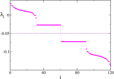
Figure 1: Entire Lyapunov spectrum $\lambda_{i}$ for an ICC. The symmetry of the spectrum with respect to $-1/2m$ is clearly visible. The data refer to $m=10$, $N=30$; the spectrum has been obtained by following the orbit and the tangent vectors for a time lapse $T_{s}=8,000$, after discarding a transient period $T_{t}=1,000$.

Furthermore, as shown in Ginelli et al. (2011) the values of the squared components $\xi_{i}^{(\sigma)}$ of the maximal Lyapunov vector ${\cal T}^{(1)}$ can give important information about the oscillators that are more actively contributing to the chaotic dynamics. The squared component for the oscillator $i$ of population $\sigma$ is measured as

$$\xi_{i}^{(\sigma)}(t)=[\delta\dot{\theta}_{i}^{(\sigma)}(t)]^{2}+[\delta{\theta}_{i}^{(\sigma)}(t)]^{2}\quad;$$ (5)

once the Lyapunov vector is normalized, i.e. $||{\cal T}^{(1)}(t)=1||$.

Moreover, the occurrence of intermittent laminar and turbulent phases, observable for ICCs, renders the characterization of the chaoticity of the system in terms of the asymptotic maximal LE extremely difficult. Therefore, for such states it is more useful to estimate the finite time Lyapunov exponents (FTLEs) $\Lambda$ over a finite time window of duration $\Delta t$, namely

$$\Lambda=\frac{1}{\Delta t}\ln\sqrt{\sum_{i=1}^{4N}\mathcal{T}_{i}^{(1)}(\Delta t)\mathcal{T}^{(1)}_{i}(\Delta t)}\enskip;$$

where the initial magnitude of the vector is set to one, i.e. $||\mathcal{T}^{(1)}(0)||\equiv 1$. In particular, we measured the associated probability distribution functions $P(\Lambda)$ by collecting $100,000$ data points for each considered system size obtained from ten different orbits, each of duration $T_{s}=100,000$ with $\Delta t=10$. The eventual presence of a peak around $\Lambda\simeq 0$ in the $P(\Lambda)$ indicates the occurrence of laminar phases, usually superimposed over a Gaussian-like profile.

In order to give an estimate of the maximal LE, we have removed from the $P(\Lambda)$ the channels eventually associated to the laminar phase, and this modified distribution has been fitted with a Gaussian function, namely $F(\Lambda)=\frac{1}{\sqrt{2\pi\sigma^{2}}}\exp{\left[\frac{(\Lambda-\Lambda^{(*)})^{2}}{2\sigma^{2}}\right]}$. The maximum of the Gaussian, $\Lambda^{(*)}$ is our best estimate of the maximal LE of the system.

From each $P(\Lambda)$ we have also obtained an estimate of the probability $p_{0}$ that the chaotic population stays in the laminar phase. In particular, $p_{0}$ has been measured by integrating $P(\Lambda)$ over the channels corresponding to $\Lambda=0$ and its nearest-neighbor channels (for a total of 3 to 5 channels).

III Stationary States

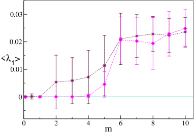
Figure 2: Average maximal LE $<\lambda_{1}>$ and the associated standard deviation vs $m$ for $N=100$: magenta diamonds (maroon stars) refer to BSCs (UCs). The averaged values $<\lambda_{1}>$ are obtained by following each realization for a time span $t=50,000$ and by averaging over 100 different initial conditions.

In this Section we analyze the different stationary states emerging in the system for different inertia values and for different initial conditions: namely, BSCs and UCs.

Starting simulations with BSCs at small inertia ($m\leq 4$), the system is not chaotic (as shown in Fig. 2) and it displays a multitude of coexisting breathing and quasiperiodic chimeras Abrams et al. (2008); Pikovsky and Rosenblum (2008). For larger inertia, the system displays not only regular but also chaotic solutions, as it can be appreciated by the fact that the maximal Lyapunov exponent, averaged over many different random realization of the initial conditions, becomes positive (see Fig. 2). In particular, for sufficiently large $m$-values ICC solutions with broken symmetry emerges. These solutions, have been previously observed experimentally and numerically in Olmi et al. (2015) and they will be characterized in detail in Sec. V.

By considering UCs, the system evolves towards chaotic solutions already at smaller inertia, namely $m>1$, as shown in Fig. 2. With these initial conditions the multistability is enhanced and many different coexisting states with broken symmetry are observable, either regular or chaotic. The chaotic ones will be examined in Sec. VI.

III.1 Broken Symmetry Initial Conditions

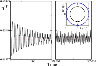
Figure 3: Order parameter $R^{(1)}$ for the non-synchronized population versus time. The red dashed curve represents the zero-inertia solution $R^{(1)}$ associated to a stationary chimera for $A=0.2$, while the black curve is $R^{(1)}$ for $m=1\times 10^{-4}$ continued from the zero-inertia state. The two panels report the evolution of $R^{(1)}$ for two successive time windows. The inset displays the real and imaginary part of the non-synchronized field $\rho^{(1)}$ corresponding to the second panel (black inner curve), while the blue dotted curve refers to $\rho^{(2)}$ associated to the fully synchronized population. The system has been integrated for a time $T_{s}=5.6\times 10^{5}$ with a time step $2\times 10^{-4}$ and $N=200$ oscillators.

III.1.1 Breathing versus Quasi-Periodic Chimeras

At zero inertia, for the considered set of parameters, a stationary chimera with a constant order parameter $R^{(1)}<R^{(2)}\equiv 1$ has been observed by Abrams et al. in Abrams et al. (2008). In order to verify the stability of the stationary chimera for finite inertia, we continued the zero-inertia solution to a sufficiently small inertia value (namely, $m_{L}$). In Fig. 3 the results of such simulation are reported, in particular the order parameter for the non-synchronized population is displayed. Due to the introduction of inertia, the order parameter is no longer constant, but it shows initally damped oscillations of extremely small amplitudes (namely, $\simeq 10^{-4}$) around the zero-inertia value. After a sufficiently long integration time, we observe that the oscillations stop to decrease and instead reveal a tendence to increase, but over very long times scales: in a time window $T=5*10^{5}$ the amplitude of the fluctuations grows of a factor 10, namely from from $6*10^{-6}$ to $1.6*10^{-5}$. As a matter of fact, after a simulation time as long as $T_{s}=5.6*10^{5}$, the system has not yet reached a stationary solution. However, for the same inertia value $m_{L}$ we obtain a completely different chimera state by following the second protocol. This solution is characterized by wide periodic oscillations of the order parameter between zero and one, as shown in Fig. 4(c).

In order to better understand the difference among these two states we have estimated for the non synchronized population the Fourier power spectra $P_{s}(\nu)$ for the real and imaginary part of the field $\rho^{(1)}$ and for its modulus $R^{(1)}$. The state obtained by the continuation of the zero-inertia solution reveals a single peak in the spectra of the real (imaginary) part of $\rho^{(1)}$ at a frequency $\nu_{1}\simeq 0.091$. Therefore, according to the definition reported in Abrams et al. (2008), this can be classified as a breathing chimera. Conversely the Fourier spectrum for the real part of the signal reported in Fig. 4(c) reveals two main peaks at uncommensurable frequencies, one at $\nu_{1}$ and a new one at $\nu_{2}\simeq 0.073$, while the Fourier spectrum of the order parameter has an unique peak at a frequency $\nu_{1}-\nu_{2}$. In this case the field is quasi-periodic, while its modulus is periodic, and this can be easily achieved by setting, e.g. $Re[\rho]=A\cos(2\pi\nu_{1}t)+B\cos(2\pi\nu_{2}t)$ and $Im[\rho]=A\sin(2\pi\nu_{1}t)+B\sin(2\pi\nu_{2}t)$. This is the only type of chimera state we have found in our simulations with BSCs by employing the second protocol and for all the considered inertia values. These can be classified as quasi-periodic chimera, according to Pikovsky and Rosenblum (2008). Due to our limited CPU resources, we cannot explore infinite times and we cannot exclude that, for sufficiently long times, the solution obtained by following the first protocol will reveal the emergence of a a second frequency $\nu_{2}$ and the state will eventually converge towards the solution obtained by following the second protocol.

If the solution is continued to inertia values larger than $m_{L}$, we observe wider oscillations around the zero-inertia stationary value. But the dynamical behaviour is the same: initially we observe damped oscillations, which, after a sufficiently long time interval, begin to show a tendency to increase again. Therefore, we can summarize our results by affirming that it is not possible to continue exactly the stationary chimeras obtained in Abrams et al. (2008). Furthermore, while the fully synchronous state remains stable also in presence of inertia, as shown in Sect. III, the stationary chimeras with constant order parameters are no longer observable at $m>0$: only breathing or quasi-periodic chimeras are present. This is probably due to the fact that the addition of inertia to the phase oscillators’ models corresponds to the addition of a degree of freedom to the system, and this is a sort of singular perturbation. Finally, we have shown that chimera states can exist for inertia values as small as $m_{L}=1*10^{-4}$, a value definitely smaller than $m=1*10^{-3}$, reported as insuperable threshold by Bountis et al. in Bountis et al. (2014). We think that the results reported in Bountis et al. (2014) should be due to integration inaccuracies and we are confident that chimera states at inertia values even smaller than $m_{L}$ can be observed, it is just a matter of employing sufficiently accurate integration schemes.

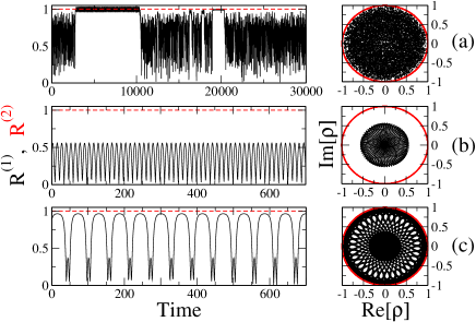
Figure 4: Left column: Order parameters $R^{(1)}(t)$ (solid black curve) and $R^{(2)}(t)$ (dashed red curve) for the two coupled populations versus time: (a) $m=10$ (chaotic chimera); (b) $m=3$ (breathing chimera); (c) $m=m_{L}$ (quasiperiodic chimera). Right column: real and imaginary parts of the fields $\rho^{(\sigma)}$ corresponding to the different dynamical states reported in the left panels. In all cases an initial transient time $T_{t}=25$ is discarded. For panels (a) and (b) the integration step is $5\times 10^{-4}$, while for panel (c) is $2\times 10^{-4}$. The systems are simulated for a time $T_{s}=5\times 10^{5}$ and $N=200$ oscillators.

III.1.2 Coexisting quasi-periodic chimeras.

By employing the second protocol with BSCs, and starting from $m=15$ the inertia is decreased to $m=m_{L}$ as explained in SubSect. II A. In the present case we have also performed a refined numerical analysis in the range $5\leq m\leq 6$ to determine the critical inertia value $m_{c}$ at which we observe the transition from chaotic to quasi-periodic chimeras, we have found $m_{c}=5$. The system shows a multitude of broken symmetry states, peculiar examples are reported in Fig. 4. For sufficiently high inertia ($5\leq m<15$) ICCs are always observable (see Fig. 4 (a)); these states will be discussed in details in Sect. V. For lower inertia values we observe only quasi-periodic chimeras of the previously described type: quasi-periodic in the macroscopic field and periodic in its modulus. Two examples are show in Fig. 4 (b) and (c) for $m=3$ and $m_{L}$, in the first case $R^{(1)}(t)$ reveals an almost sinusoidal shape, while in the other case not.

Furthermore, the system is multistable, for different initial conditions a multitude of coexisting quasi-periodic states are observable. A few examples are reported in Fig.  5 for $m=3$ and 5. At the lower inertia value $m=3<m_{c}$ non chaotic quasi-periodic chimeras are present with different periods and level of synchronization, while for $m=5$ non chaotic quasi-periodic chimeras coexist with ICCs.

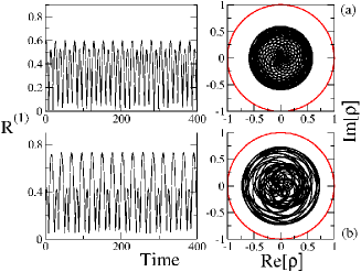
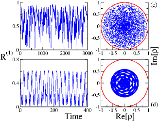
Figure 5: Left panels: Order parameter of the non-synchronized family as a function of time for different BSCs. The order parameter of the synchronized family is not shown. Right panels: imaginary vs real part of the complex fields $\rho^{(1)}$ and $\rho^{(2)}$ for $m=3$ (panels (a),(b)) and for $m=5$ (panels (c),(d) ). In all cases a time step $5\times 10^{-4}$ is used and an initial transient time $T_{t}=25$ is discarded. The systems are simulated for a time $T_{s}=5\times 10^{5}$ and $N=200$ oscillators.

III.2 Uniform Initial Conditions

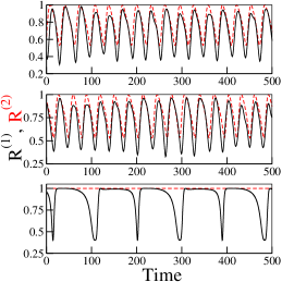
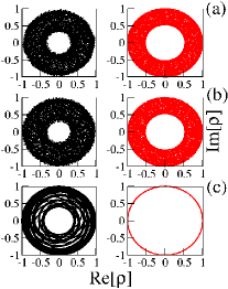
Figure 6: Left panels: Order parameters $R^{(1)}$ (black solid line) and $R^{(2)}$ (red dashed line) vs time; Right panels: imaginary vs real part of the complex fields $\rho^{(1)}$ and $\rho^{(2)}$ for (a) $m=10$; (b) $m=9$; (c) $m=3$. In all cases a time step $5\times 10^{-4}$ is used and an initial transient time $T_{t}=25$ is discarded. The systems are simulated for a time $T_{s}=100,000$ and for $N=200$.

By following the second protocol with UCs, the inertia value is decreased from $m=15$ to $m_{L}$ as explained in SubSect. II A. Also with UCs the system shows a moltitude of broken symmetry states, as shown in Fig. 6. In particular, C2P solutions are always present in the range $5\leq m\leq 15$. These states are characterized by an irregular behavior of both order parameters and the dynamics of the two populations takes place on different macroscopic attractors, as it is clearly observable in Fig. 6 (a) and (b). These states will be discussed in details in Sec. V. In the intermediate inertia range $3\leq m<5$ the system exhibits broken symmetry states, where the macroscopic field is quasi-periodic and its modulus is periodic. Even though the macroscopic field shows an almost regular behavior, a weak chaoticity is still present (see Fig  6 (c)). This residual chaoticity seems to be related to the distortion in amplitude of the macroscopic field and can be observed only following the second protocol with UCs. Finally for smaller inertia values $(m_{L}\leq m<3)$ only the fully synchronous state is present.

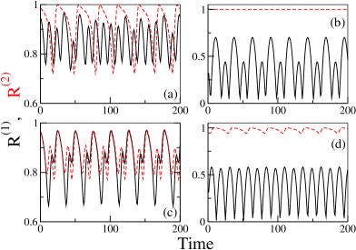
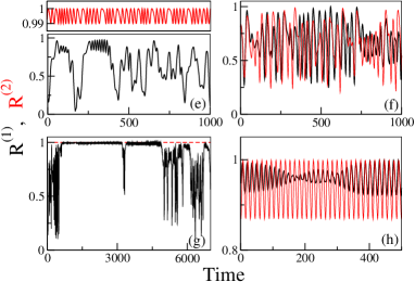
Figure 7: Order parameters $R^{(1)}$ (black solid line) and $R^{(2)}$ (red dashed or solid line) vs time for different UCs. Panels (a)-(d) refer to $m=3$. Panels (e)-(h) refer to $m=10$. The systems are simulated for a time $T_{s}=100,000$ and for $N=200$.

The system is highly multistable; in particular, if it is initialized at $m=3$ and 2 with UCs, without following any protocol, quasi-periodic chimeras with no residual chaoticity (Fig.  7 (b)) coexist with C2P solutions (Fig.  7 (a)) and with generalized broken symmetry states (Fig.  7 (c), (d)), where both macroscopic fields are quasi-periodic, but the level of synchronicity is different for the populations. Conversely at $m=10$, C2Ps can be observed (Fig.  7 (f), (h)) as well as ICCs (Fig.  7 (g)) and a novel chaotic brooken symmetry state (Fig.  7 (e)), where both population are chaotic, but one population shows also intermittency.

IV Intermittent Chaotic Chimeras

In this Section, we want to better characterize the dynamics of ICCs, observable with BSCs, already reported in Fig. 4 (a). The chaotic population exhibits clear intermittent behavior (see Fig. 9(a)), displaying a laminar phase where the two populations tend to synchronize, and a turbulent phase, where the order parameter behaves irregularly. In particular, during laminar phases, the non-synchronized order parameter stays in proximity of value one, displaying small oscillations. Furthermore, as we will show in the following the ICCs are transient, but we have been unable to find with BSCs and for the same inertia coexisting ICCs associated to different chaotic attractors.

A further indication of the presence of intermittency can be given by the estimation of the power spectrum $P_{s}(\nu)$ of the incoherent order parameter (see Fig. 8). We observe that $P_{s}(\nu)$ approaches the limit of low frequencies as $1/\nu$, as expected for an intermittent system Manneville (1980). In particular, Manneville in Manneville (1980) reported a detailed analysis of a discrete dissipative dynamical system displaying intermittency, revealing that a $1/\nu$ spectrum is typically associated to a system exhibiting a transition to turbulence via an intermittency route.

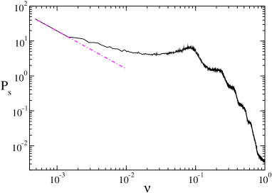
Figure 8: Power spectrum $P_{s}(\nu)$ of the chaotic order parameter as a function of the frequency $\nu=1/T$ for an ICC. Red dashed line: $y=1.06\nu^{-1.09}$. Data refer to $m=10$, $N=200$. The spectrum $P_{s}$ is obtained by following each realization for a time span $t=100,000$ and by averaging over 100 different initial conditions.

IV.1 Finite Time Lyapunov Analysis

The presence of alternating erratic and laminar phases makes difficult to employ the usual maximal Lyapunov Exponent to characterize the dynamics of the ICCs, therefore to analyse the stability of this regime we prefer to determine the distribution $P(\Lambda)$ of the FTLE $\Lambda$. As a first result, we can affirm that a non chaotic behaviour is associated to the laminar phases, in fact during these phases $\Lambda$ is almost zero as shown Fig. 9(b). This reflects in the appearence of a peak around $\Lambda=0$ in the distribution $P(\Lambda)$, as observable in the inset of Fig. 10 (a). In more details, the laminar phases are characterized by the synchronization of most part of the oscillators belonging to the chaotic population, which get entrained to the synchronized population. This can be understood looking at Fig. 9(c), where the frequencies of two typical oscillators, one belonging to the chaotic and the other to the synchronized population, are reported during chaotic and laminar phases. These two oscillators (as the majority of the oscillators) synchronize during the laminar phases, as observable by the fact that their frequencies approach the constant average value associated to the fully synchronized regime, namely $\bar{\omega}=1-\frac{1}{2}\sin\gamma$. However, a few oscillators of the chaotic population do not get synchronized to all the others during the laminar phases. Instead, they start oscillating with an unique frequency but with incoherent phases, giving rise to the oscillations observable in the order parameter and, thus, contributing to desynchronize the system. When the laminar phase ends, all the oscillators in the chaotic population return to behave irregularly.

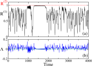
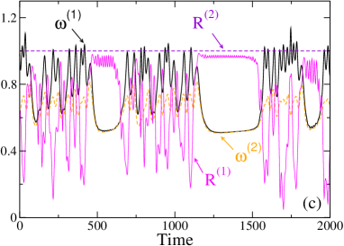
Figure 9: (a) Order parameters $R^{(1)}(t)$ (solid black curve) and $R^{(2)}(t)$ (dashed red curve) for the ICCs as a function of time. (b) FTLE $\Lambda$ for the chaotic population versus time. (c) The solid black (dashed orange) curve represents the frequency $\omega^{(1)}$ ($\omega^{(2)}$) of a single oscillator belonging to the chaotic (synchronized) population as a function of time; the solid magenta (dashed violet) curve represents its respective order parameter $R^{(1)}(t)$ ($R^{(2)}(t)$). All simulations are referred to $m=10$, $N=200$.

To characterize the degree of chaoticity of the erratic phase, we should give an estimate of the average Lyapunov exponent $\Lambda^{(*)}$ restricted to this phase. We proceeded as explained in Sect. II B, and as previously done in Olmi et al. (2015), in particular $\Lambda^{(*)}$ represents the maximum value of the probability distribution function $P(\Lambda)$ (shown in the inset of Fig. 10(a)), once removed the peak around $\Lambda=0$ characteristic of the laminar phase. It is interesting to examine the dependence of $\Lambda^{(*)}$ on the system size. In particular, one can observe a clear decrease of $\Lambda^{(*)}$ with the system size, namely as $1/\ln(N)$ as clearly shown in Fig. 10(a). Furthermore, from these data one can extrapolate the value of $\Lambda^{(*)}$ in the thermodynamic limit, which is definitely positive, namely $\Lambda^{(*)}\simeq 0.022$. Therefore, we can affirm that the ICCs remain chaotic for coupled rotators even for $N\to\infty$, at variance with the weak chaotic regime observed for the Kuramoto model in Wolfrum et al. (2011); Popovych et al. (2005). The logarithmic dependence of the maximal LE $\lambda_{M}$ with the system size has been previously found for globally coupled dissipative systems in Takeuchi et al. (2011), where, the authors have shown analytically that

$$\lambda_{M}(N)=\lambda_{mf}+\frac{D}{2}+\frac{a}{\ln(N)}+{\cal O}\left(\frac{1}{\ln^{2}(N)}\right)\enskip;$$ (6)

where $\lambda_{mf}$ is the mean field LE obtained by considering an isolated unit of the chaotic population forced by the fields $\rho^{(\sigma)}$, $D$ is the diffusion coefficient associated to the fluctuations of $\lambda_{mf}$. As explained in Appendix A, these quantities can be numerically estimated giving $\lambda_{mf}\simeq 0.0116(5)$ and $D\simeq 0.0180(10)$, therefore in our case the expected asymptotic Lyapunov exponent should be $\lambda_{M}(\infty)\simeq 0.021(1)$, which is in good agreement with the previously reported numerical extrapolation, as shown in Fig. 10(a).

A more detailed analysis of the stability of the chaotic phase can be attained by estimating the Lyapunov spectra for different sizes. The spectrum (see upper inset in Fig.  10(b)) is composed by a positive part made of $N-2$ exponents and a negative part composed of $N$ exponents. Moreover two exponents are exactly zero: one is always present for systems with continuous time, while the second arises due to the invariance of Eq. (1) for uniform phase shifts. In particular the negative part of the spectrum is composed by $N-1$ identical exponents, which measure the transverse stability of the synchronous solution, plus an isolated LE, which expresses the longitudinal stability of the synchronized population (as explained in Appendix B). The transverse stability can be obtained by estimating the mean field LE associated to the synchronized family; the agreement with the numerical data is perfect as shown in the inset of Fig. 10(b) (for more details see Appendix A). Furthermore, the central part of the positive spectrum tends to flatten towards the mean field value $\lambda_{mf}$ for increasing system sizes (see Fig. 10(b) for N =100; 200; 400 and 800), while the largest and smallest positive LEs tend to split, in the same limit, from the rest of the spectrum. This scaling of the Lyapunov spectra has been found to be a general property of fully coupled dynamical systems in  Takeuchi et al. (2011); Ginelli et al. (2011), where it has been shown that the spectrum becomes asymptotically flat (thus trivially extensive) in the thermodynamic limit, but this extensive part is squeezed between the largest and smallest LEs, which constitute two subextensive bands of order ${\cal O}(\log N)$. This scaling behavior, typical of fully coupled system, is in contrast with the results reported for chaotic chimeras in  Wolfrum and Omel’chenko (2011); Wolfrum et al. (2011), where the ring geometry strongly influences the stability properties, thus indicating the dependence of the results for chaotic chimeras on the underlying network topology.

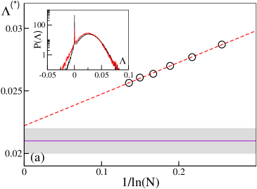
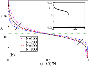
Figure 10: (a) Plot of $\Lambda^{(*)}$ (symbols) versus $1/ln(N)$ for $100\leq N\leq 1600$ and the corresponding fit. The continue violet curve with the shaded area denotes $\lambda_{M}(\infty)$ with its error bar. Inset: Probability distribution function $P(\Lambda)$ for $N=150$ (black curve) and 1600 (red curve). (b) Positive part of the Lyapunov spectra for various sizes, the dotted green line is $\lambda_{mf}$. Upper inset: Lyapunov spectrum for $N=100$. The dashed line denotes the mean field LE that can be estimate by using Eqs. (7) and (8) for the synchronized population.

IV.2 Life-time of ICCs

By measuring the life time of chaotic chimeras we have found that ICCs are transient states; in particular we observed for different inertia that chaotic chimeras converge to a regular (non-chaotic) state after a transient time $\tau$. In particular we have observed that ICCs decay either to a fully synchronized state or to a quasiperiodic chimera.

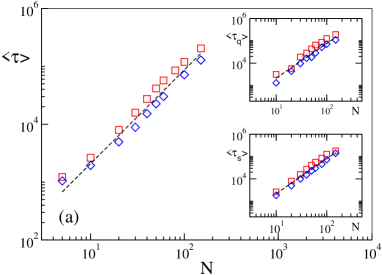
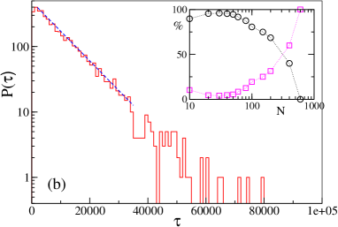
Figure 11: (a) Average life-time $<\tau>$ of ICCs vs $N$ for $m=10$ (red squares) and $m=8$ (blue diamonds). The black dashed line refers to a power law with exponent 1.60. In the insets are shown, for the same $m$ values, the partial results for the chaotic chimeras that decay in a stable quasiperiodic chimera (upper inset) or in a fully synchronized state (lower inset). The black dashed line in the upper (lower) inset refers to a power law with exponent 1.55 (1.56). Data are averaged over 200-4000 different realizations of BSCs. (b) Distribution $P(\tau)$ of the life-times $\tau$ of ICCs for $N=30$ and $m=6$ obtained from 4,000 data. The dashed blue curve is an exponential fit with a decay time $\tau^{*}=9,590(5)$. Inset: percentage of states decaying towards a synchronized state (black circles) or towards a quasiperiodic chimera (magenta squares) as a function of the systems size.

By measuring the average life times $<\tau>$ for two inertia values, namely $m=8$ and 10, and various system sizes $5\leq N\leq 150$, we have found a power-law divergence of the decaying time with an exponent $\alpha\simeq 1.60(5)$ for $N\geq 10$ (see Fig. 11(a)). Furthermore the power law divergence is still present if we consider separately the average life times $<\tau_{q}>$ ($<\tau_{s}>$) of ICCs decaying in a quasiperiodic chimera (synchronized state), as shown in the upper (lower) inset in Fig. 11(a). Even though we were unable to verify that this scaling is present over more than one decade, due to computational problems, we can safely affirm that these times are not diverging exponentially with the size as reported in Wolfrum and Omel’chenko (2011). This is a further indication that the topology presently considered deeply influences the nature of the observed phenomenon.

The life time distribution $P(\tau)$, obtained for different initial conditions, is exponential: as shown in Fig. 11(b) for $N=30$ and $m=6$. The exponential decay can be fitted as $exp(-t/\tau^{*})$, where the decay time $\tau^{*}\simeq 9,590$ is consistent with average life time value obtained for the same size and inertia, namely $\langle\tau\rangle>\simeq 9,975$. Thus indicating that this can be described as a Poisson process. Moreover chaotic chimeras can preferentially decay to the synchronized state or to a broken symmetry state depending on the system size. In particular, for small sizes the decay to a synchronized state is preferred, while for larger sizes, ICCs decay more probably to a quasiperiodic chimera (as shown in the inset of Fig.  11(b)). Finally, we have tested the dependence of $\langle\tau\rangle$ on the inertia, for two system sizes, namely $N=30$ and 50 and we have observed that $\langle\tau\rangle$ is diverging as a power law with $m$ with exponents $\simeq 2-3$, as reported in Fig. 12.

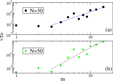
Figure 12: Average life time $\langle\tau\rangle$ vs inertia for $N=30$ (a) and 50 (b). The blue (maroon) dashed line in panel (a) (panel (b)) refers to a power law with exponent 2.38(5) (2.98(5)). The values of $\langle\tau\rangle$ are averaged over 3000 different realizations of BSCs.

V Chaotic Two Populations

In this Section the microscopic dynamics of stationary states emerging with UCs is characterized. For high inertia values both populations are usually chaotic but their dynamics takes place on different macroscopic chaotic attractors, thus giving rise to broken symmetry C2P states. Two examples are reported in in Figs. 6 (a) and (b). However, at variance with ICCs, C2Ps are not intermittent neither transient.

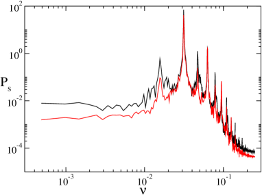
Figure 13: Power spectra $P_{s}$ as a function of $\nu$ for the two order parameters associated to the C2Ps state reported in Fig. 6 (a). The spectra $P_{s}$ are obtained by following each realization for a time span $T_{s}=100,000$ and by averaging over 100 different initial conditions. Data refer to $m=10$, $N=200$.

To better characterize the C2Ps state, we have estimated the power spectra $P_{s}(\nu)$ associated with the order parameters $R^{(1)}$ and $R^{(2)}$ for the state shown in Fig. 6 (a). These spectra, reported in Fig. 13, Fig. 6 (a) show an almost flat behavior at low frequencies, thus being strongly different from the spectrum of the ICCs shown in Fig. 8. In particular, each spectrum resembles a Lorentzian with several subsidiary peaks associated to harmonics and subharmonics of a fundamental frequency $\nu_{0}\simeq 0.03125$ ($T_{0}=1/\nu_{0}=32$). The main peak, corresponding to $T_{0}$, is related to the mean period of the oscillations observable in the order parameters.

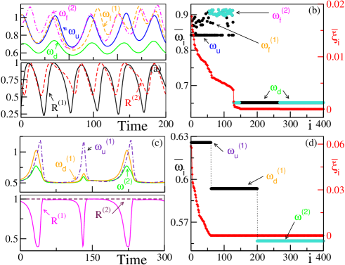
Figure 14: Frequencies $\omega^{(1)}$ ($\omega^{(2)}$) of oscillators belonging to population $\sigma=1$ ($\sigma=2$) as a function of time, and the corresponding order parameter $R^{(1)}(t)$ ($R^{(2)}(t)$) for $m=9$ (a) and $m=3$ (c). Average components of the vector $\left\{\bar{\xi}_{i}\right\}$ (red diamonds) together with the corresponding average frequencies of the oscillators $\bar{\omega}_{i}$ for population one (black circles) and two (turquoise circles), for $m=9$ (b) and $m=3$ (d). The indeces of the rotators are ordered accordingly to the value of $\bar{\xi}_{i}$. For more details on the hightlighted frequencies see the text. Data in panels (a) and (c) are referred to the state shown in Fig. 6 (b) and in panels (b) and (d) to the one reported in Fig. 6 (c). The time averages have been performed over a time interval $T_{s}\simeq 5\times 10^{4}$.

Moreover, the C2P states are characterized by different amplitude evolution of $R^{(1)}$ and $R^{(2)}$, being the differences due to the different number of isolated oscillators present in the two populations. In fact, oscillators of both populations share at least one common cluster, characterized by a common average frequency, and the erratic dynamics is induced by the evolution of non clustered oscillators belonging to both populations. Let us examine for example the C2P state reported in Fig. 6 (b) for $m=9$. As shown in Fig. 14(b) the oscillators split in a common cluster plus a second cluster belonging to one population only and few non synchronized oscillators. The frequencies of the oscillators of the two populations belonging to the lower cluster $\omega_{d}$ are identical, while the frequencies belonging to the upper cluster $\omega_{u}$ are locked to those of the lower cluster; thus the two order parameters show similar oscillation periods as reported in Fig. 14(a). However, the oscillators belonging to the upper cluster and few oscillators out of the clusters $\omega^{(\sigma)}_{f}$ ensure the microscopic dynamics to be chaotic, as can be proved by estimating the time averaged contribution $\bar{\xi}_{i}$, of the $i-$th oscillator, to the modulus of the maximal Lyapunov vector. In particular, as shown in Fig.  14(b) the contribution $\bar{\xi}_{i}$ of the oscillators belonging to the common cluster is essentially negligible and the only relevant contributions comes from the oscillators with higher, non common, average frequencies. These states resemble imperfect chimeras recently observed in experiments on coupled metronomes Kapitaniak et al. (2014) and in simulations of chains of Kuramoto oscillators with inertia Jaros et al. (2015).

For low inertia values many states arise with different level of chaoticity. In Fig.  14(c) and (d) the case shown in Fig. 6 (c) for $m=3$ is analyzed. In this example, one has a synchronized population and a second population with an almost regular behaviour, as discussed previously in Sect. IV. Let us try to understand the origing of the residual chaoticity in the second population, the oscillators belonging to the synchronized population share the same average frequency $\omega^{(2)}$, while the other population breaks up into two clusters: a lower one at frequency $\omega^{(1)}_{d}$ and an upper one at larger frequency $\omega^{(1)}_{u}$. As shown in Fig.  14(d) the only relevant contribution to maximal Lyapunov vector is due to the oscillator with higher frequencies, as in the previous case, i.e. to the one belonging to the upper cluster.

VI Conclusions

In this work, we have characterized in details the dynamical properties of different symmetric or symmetry broken states emerging in a simple numerical model of heterogeneously coupled oscillators with inertia. The presence of inertia is a distinctive ingredient to observe the emergence of chaotic regimes. While for small inertia values, quasi-periodic (or in rare cases, breathing) chimeras coexist with the fully synchronized state, at large inertia values, two types of chaotic solutions are found depending on the initial conditions. For uniform initial conditions Chaotic Two Population states are observable, where the erratic dynamics is induced by the evolution of the non clustered oscillators belonging to both populations. On the other hand, both for initial conditions with a broken symmetry as well as for uniform initial conditions, Intermittent Chaotic Chimeras can emerge. For ICCs the chaotic population exhibits turbulent phases interrupted by laminar regimes. While C2Ps are stable solutions, ICCs are transient states and their life-times diverge as a power-law with the size and the inertia value. Therefore, in the thermodynamic limit these states survive for infinite time. Moreover the Lyapunov analyses reveal chaotic properties in quantitative agreement with theoretical predictions for globally coupled dissipative systems Takeuchi et al. (2011).

Chimera states have been initially observed in spatially extended systems with long-range coupling and, so far, this configuration has been considered analogous to its limit case represented by two globally coupled sub-populations with heterogeneous coupling  Abrams et al. (2008). We clearly demonstrate that chaotic chimeras observed in spatially extended systems in  Wolfrum and Omel’chenko (2011); Wolfrum et al. (2011) have completely different dynamical properties with respect to fully coupled sub-populations. This means that the relevance of the network topology for the stability properties of the chimera states, in particular of chaotic ones, has been so far overlooked and it suggests that also regular chimeras could reveal different stability properties related to the underlying topology.

Finally, due to the introduction of inertia, stationary chimera states characterized by a fully synchronized population and a partially synchronized one, are no longer observable. In particular, performing a numerical continuation of the zero-inertia solution, we have shown that stationary chimeras cannot be continued to finite inertia. Instead, the continuation procedure give rises to breathing or quasi-periodic chimeras. This is probably due to the fact that the introduction of inertia corresponds to the addition of a new degree of freedom, thus giving rise to a singular perturbation of the dynamics.

Appendix A Finite Size Scaling of the Maximal Lyapunov Exponent

The mean field evolution of an oscillator $\phi^{(\sigma)}$ belonging to the population $\sigma$ for the considered model can be obtained by assuming that the influence of the oscillator on the network dynamics is negligible, while its dynamics is driven by the fields $\rho^{(1)}$ and $\rho^{(2)}$, associated to the two populations, which are treated as external forcing fields. In particular, the mean field dynamics for an oscillator of population $\sigma$ can be written as

$$m\ddot{\phi}^{(\sigma)}+\dot{\phi}^{(\sigma)}=\Omega+\sum_{\sigma^{\prime}=1}^{2}K_{\sigma\sigma^{\prime}}\left\{Im\left[\rho^{(\sigma^{\prime})}\right]\cos(\phi^{(\sigma)}+\gamma)\right.$$

$$\left.-Re\left[\rho^{(\sigma^{\prime})}\right]\sin(\phi^{(\sigma)}+\gamma)\right\}\enskip.$$ (7)

If we linearize the previous equation we can obtain the evolution of an infinitesimal perturbations in the tangent space

$$m\delta\ddot{\phi}^{(\sigma)}+\delta\dot{\phi}^{(\sigma)}=-\sum_{\sigma^{\prime}=1}^{2}K_{\sigma\sigma^{\prime}}\left\{Im\left[\rho^{(\sigma^{\prime})}\right]\sin(\phi^{(\sigma)}+\gamma)\right.$$

$$\left.+Re\left[\rho^{(\sigma^{\prime})}\right]\cos(\phi^{(\sigma)}+\gamma)\right\}\delta\phi^{(\sigma)}\enskip.$$ (8)

Furthermore, using Equations (7) and (8), we have estimated numerically the associated maximal LE by applying the standard method reported in Benettin et al. (1980). For each population $\sigma$ it is possible to find a maximal mean field LE $\lambda_{0}^{(\sigma)}$. For the numerical integrations of Eqs (7) and (8) we have employed the fields $\rho^{(1)}(t)$ and $\rho^{(2)}(t)$ obtained by simulating at the same time a two population network made of $2N$ oscillators. In particular, for the ICC state where $\sigma=1$ ($\sigma=2$) is the chaotic (synchronized) population, $\lambda_{0}^{(1)}$ ($\lambda_{0}^{(2)}$) is positive (negative); the mean field exponent $\lambda_{0}^{(2)}$ corresponds to the transverse LE for the synchronized population and it is analogous to the one discussed in Appendix B in the case of full synchronization of both populations (see Fig. 15). While $\lambda_{0}^{(1)}$ is the value to which the most part of the positive LEs, associated to the chaotic population, tends for increasing system sizes, and it has been indicated in Sec. IV as $\lambda_{mf}$ (see Fig. 10 (b)).

For fully coupled dissipative systems, made of a single population of chaotic units, it has been demonstrated in Takeuchi et al. (2011) that in the thermodynamic limit the most part of the Lyapunov spectrum becomes flat assuming the value of the mean field LE for the considered system. Only a few LEs ${\cal O}(\ln N)$, locate at the extrema of the spectrum, corresponding to the largest (smallest) values, exhibit different asymptotic values. In particular, it has been shown that the maximal LE scale as

$$\lambda_{M}=\lambda_{mf}+\frac{D}{2}+\frac{a}{\ln(N)}+{\cal O}\left(\frac{1}{\ln^{2}(N)}\right)\enskip,$$ (9)

where $\lambda_{mf}$ is the mean field LEs, and $D$ is the diffusion coefficient associated to the fluctuations of the instantaneous mean field LE.

In particular, $D$ takes into account the effect of the coupling with the other oscillators neglected in the estimation of the mean field LE; in order to estimate $D$ one has to measure the mean square displacement of the following quantity $[\ln d(t)-\lambda_{mf}t]$, where $d(t)=\sqrt{|\delta\dot{\phi}^{(1)}(t)|^{2}+|\delta{\phi}^{(1)}(t)|^{2}}$ is the modulus of the infinitesimal vector appearing in Eq. (8). Therefore for sufficiently long times one expects to observe the following scaling

$$[\ln d(t)-\lambda_{mf}t]^{2}=Dt,$$ (10)

where $d(0)=1$. In Olmi et al. (2015) we have shown that the scaling reported in Eq. (9) is optimally reproduced by the maximal LE measured for our system composed of two populations and presenting a broken symmetry. Furthermore, whenever we substitute $\lambda_{mf}$ with $\lambda_{0}^{(1)}$ in Eq. (9) and Eq. (10), the Eq. (9) gives also a very good estimate of the value attained by the maximal LE in the thermodynamic limit, as shown in Olmi et al. (2015). These results confirm the validity of the theoretical estimate reported in Takeuchi et al. (2011) also for system composed by more than one population, and where the collective dynamics is represented by more than a single macroscopic field.

Appendix B Linear Stability of the Synchronized State

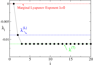
Figure 15: Lyapunov spectrum $\lambda_{i}$ for the fully synchronized state. Analytical values: the marginal LE (dashed red line) corresponds to the maximal LE; the longitudinal LE $\lambda^{(L)}$ (dashed blue line) to the second exponent and the transverse LE $\lambda^{(T)}$ (dashed green line) to the last $2N-2$ degenerate exponents. The results of the numerical simulations are shown as black circles. The data refer to $m=10$ and $N=10$.

It is instructive to derive analytically the LEs for the fully synchronized solution. Whenever the system is fully synchronized, Eq. (3) can be simplified by noticing that $\theta_{i}^{(1)}=\theta_{j}^{(2)}$ $\forall i,j$. Thus, Eq. (3) becomes

$$m\enskip\delta\ddot{\theta}_{i}^{(\sigma)}+\delta\dot{\theta}_{i}^{(\sigma)}=\sum_{\sigma^{\prime}=1}^{2}\frac{K_{\sigma\sigma^{\prime}}}{N}\cos(\gamma)\sum_{j=1}^{N}(\delta\theta_{j}^{(\sigma^{\prime})}-\delta\theta_{i}^{(\sigma)}).$$ (11)

Moreover it is useful to rewrite Eq. (11) as follows:

$$m\enskip\delta\ddot{\theta}_{i}^{(\sigma)}+\delta\dot{\theta}_{i}^{(\sigma)}=-\frac{\cos(\gamma)}{2}\delta\theta_{i}^{(\sigma)}+\frac{\mu\cos(\gamma)}{N}\delta\theta_{i}^{(\sigma)}$$ (12)

$$+ \frac{\mu}{N}\cos(\gamma)\sum_{j\neq i}\delta\theta_{j}^{(\sigma)}+\frac{\nu}{N}\cos(\gamma)\sum_{j=1}^{N}\delta\theta_{j}^{(\sigma^{\prime})}.$$

where now $\sigma\neq\sigma^{\prime}$ is 1 or 2.

Starting from the previous equation it is possible to calculate both the longitudinal $\lambda^{(L)}$ and the transverse LE $\lambda^{(T)}$ Heagy et al. (1995), which are usually employed to characterize a synchronized system. In general, even a chaotic state which displays a positive $\lambda^{(L)}$ can be fully synchronized, whenever all the transverse LEs are negative Pikovsky et al. (2002). In the present case the shape of the Lyapunov spectrum $\{\lambda_{i}\}$, limited to the first half $i=1,\dots,2N$ is shown in Fig. 15. In the system under investigation one might expect two zero LE: one is always present for system with continuous time while the second zero LE is due to the invariance of the model under uniform phase shift. The figure reveals only one zero LE, instead of two as one might expect: the phase shift of all the phases corresponds to a perturbation along the orbit of the fully synchronized state, which explains why the two invariances, and thus LEs, coincide. Furthermore, one observes an isolated LE and a plateau of $2N-2$ identical exponents.

The first two exponents correspond to longitudinal exponents, while the $2N-2$ identical exponents correspond to transverse exponents.

The longitudinal exponents can be estimated by considering the average of all the perturbations $Z^{(\sigma)}=\frac{1}{N}\sum_{j=1}^{N}\delta\theta_{j}^{(\sigma)}$ whose evolution is ruled by

$$m\ddot{Z}^{(\sigma)}+\dot{Z}^{(\sigma)}=\cos(\gamma)\left[(\mu-\frac{1}{2})Z^{(\sigma)}+\nu Z^{(\sigma^{\prime})}\right]\enskip,$$ (13)

and the associated eigenvalue equation reads as

$$\left[m(\lambda^{(L)})^{2}+\lambda^{(L)}\right]\left(\begin{array}[]{c}Z^{(1)}\\ Z^{(2)}\end{array}\right)=$$ (16)

$$\left(\begin{array}[]{cc}\cos(\gamma)(\mu-\frac{1}{2})&\nu\cos(\gamma)\\ \nu\cos(\gamma)&\cos(\gamma)(\mu-\frac{1}{2})\end{array}\right)\left(\begin{array}[]{c}Z^{(1)}\\ Z^{(2)}\end{array}\right),$$ (21)

yielding two second order secular equations

$$m(\lambda^{(L)})^{2}+\lambda^{(L)}=0\enskip,\qquad m(\lambda^{(L)})^{2}+\lambda^{(L)}+2\cos(\gamma)\nu=0\enskip.$$

Each of the above equations admits two solutions that are symmetric with respect to $-1/2m$. The largest LEs are

$$\lambda^{(L)}=0\enskip,\qquad\lambda^{(L)}=\frac{-1+\sqrt{1-8m\nu\cos(\gamma)}}{2m}.$$

The marginal LE, $\lambda^{(L)}=0$, is associated to a neutral perturbation along the orbit, while the real part of the second longitudinal exponent is always negative. Therefore the achieved orbit is stable, provided that $m,\nu<\infty$ are finite and $\gamma\neq\pi/2$.

On the other hand, the transverse LE can be estimated by considering the evolution of the difference between two infinitesimal perturbations associated with two generic oscillators $i$ and $j$ of the same population, namely $W^{(\sigma)}=\delta\theta_{j}^{(\sigma)}-\delta\theta_{i}^{(\sigma)}$. Using (12), its temporal evolution is given by

$$m\ddot{W}^{(\sigma)}+\dot{W}^{(\sigma)}=-\frac{\cos(\gamma)}{2}W^{(\sigma)}.$$ (22)

The associated secular equation reads

$$m(\lambda^{2}-\Omega^{2})+\lambda=-\frac{\cos(\gamma)}{2}\enskip,$$

and is easily solved, yielding the maximal transverse LE

$$\lambda^{(T)}=\frac{-1+\sqrt{1-2m\cos(\gamma)}}{2m}$$

whose real part is always negative for any finite inertia, provided that $\gamma\neq\pi/2$.

The analytic predictions are in perfect agreement with the simulation results for a fully synchronized state, as shown in Fig. 15. Furthermore, our analysis ensures that this state is always a stable solution for the system, given a finite inertia $m<\infty$, $A<1$ and a phase lag $\gamma\neq\pi/2$.

Whenever the phase lag is exactly equal to $\pi/2$, $\lambda^{(L)}=\lambda^{(T)}=0$ and the system becomes highly degenerate, thus resembling the completely integrable dynamics of phase oscillators with global cosine coupling studied in Watanabe and Strogatz (1993).

References

- Motter (2010) A. E. Motter, Nature Physics 6, 164 (2010).
- Panaggio and Abrams (2015) M. J. Panaggio and D. M. Abrams, Nonlinearity 28, R67 (2015).
- Ermentrout (1991) B. Ermentrout, Journal of Mathematical Biology 29, 571 (1991).
- Tanaka et al. (1997a) H.-A. Tanaka, A. J. Lichtenberg, and S. Oishi, Physical review letters 78, 2104 (1997a).
- Tanaka et al. (1997b) H.-A. Tanaka, A. J. Lichtenberg, and S. Oishi, Physica D: Nonlinear Phenomena 100, 279 (1997b).
- Ji et al. (2013) P. Ji, T. K. D. Peron, P. J. Menck, F. A. Rodrigues, and J. Kurths, Phys. Rev. Lett. 110, 218701 (2013).
- Gupta et al. (2014) S. Gupta, A. Campa, and S. Ruffo, Physical Review E 89, 022123 (2014).
- Komarov et al. (2014) M. Komarov, S. Gupta, and A. Pikovsky, EPL (Europhysics Letters) 106, 40003 (2014).
- Olmi et al. (2014) S. Olmi, A. Navas, S. Boccaletti, and A. Torcini, Physical Review E 90, 042905 (2014).
- Trees et al. (2005) B. Trees, V. Saranathan, and D. Stroud, Physical Review E 71, 016215 (2005).
- Salam et al. (1984) F. Salam, J. E. Marsden, and P. P. Varaiya, Circuits and Systems, IEEE Transactions on 31, 673 (1984).
- Filatrella et al. (2008) G. Filatrella, A. H. Nielsen, and N. F. Pedersen, The European Physical Journal B 61, 485 (2008).
- Rohden et al. (2012) M. Rohden, A. Sorge, M. Timme, and D. Witthaut, Physical review letters 109, 064101 (2012).
- Motter et al. (2013) A. E. Motter, S. A. Myers, M. Anghel, and T. Nishikawa, Nature Physics 9, 191 (2013).
- Huygens (1967) C. Huygens, Oeuvres Completes (Swets & Zeitlinger Publishers, Amsterdam, 1967).
- Strogatz et al. (2005) S. H. Strogatz, D. M. Abrams, A. McRobie, B. Eckhardt, and E. Ott, Nature 438, 43 (2005).
- Wiesenfeld et al. (1998) K. Wiesenfeld, P. Colet, and S. Strogatz, Physical Review E 57, 1563 (1998), ISSN 1063-651X.
- Michaels et al. (1987) D. Michaels, E. Matyas, and J. Jalife, Circ. Res. 61, 704 (1987).
- Liu et al. (1997) C. Liu, D. R. Weaver, S. H. Strogatz, and S. M. Reppert, Cell 91, 855 (1997), ISSN 00928674.
- Kiss et al. (2002) I. Z. Kiss, Y. Zhai, and J. L. Hudson, Science (New York, N.Y.) 296, 1676 (2002).
- Danøet al. (1999) S. Danø, P. G. Sø rensen, and F. Hynne, Nature 402, 320 (1999), ISSN 0028-0836.
- Massie et al. (2010) T. M. Massie, B. Blasius, G. Weithoff, U. Gaedke, and G. F. Fussmann, Proceedings of the National Academy of Sciences of the United States of America 107, 4236 (2010).
- Buzsaki (2006) G. Buzsaki, Rhythms of the Brain (Oxford University Press, 2006).
- Uhlhaas and Singer (2006) P. J. Uhlhaas and W. Singer, Neuron 52, 155 (2006).
- Kuramoto and Battogtokh (2002) Y. Kuramoto and D. Battogtokh, Nonlinear Phenomena in Complex Systems 5, 380 (2002).
- Abrams and Strogatz (2004) D. M. Abrams and S. H. Strogatz, Physical review letters 93, 174102 (2004).
- Shima and Kuramoto (2004) S. I. Shima and Y. Kuramoto, Phys. Rev. E 69, 036213 (2004).
- Abrams et al. (2008) D. M. Abrams, R. Mirollo, S. H. Strogatz, and D. A. Wiley, Physical review letters 101, 084103 (2008).
- Martens (2010) E. A. Martens, Physical Review E 82, 016216 (2010).
- Omel’chenko et al. (2008) O. E. Omel’chenko, Y. L. Maistrenko, and P. A. Tass, Physical Review Letters 100, 044105 (2008).
- Pikovsky and Rosenblum (2008) A. Pikovsky and M. Rosenblum, Phys. Rev. Lett 101, 264103 (2008).
- Olmi et al. (2010) S. Olmi, a. Politi, and a. Torcini, EPL (Europhysics Letters) 92, 60007 (2010).
- Laing (2009a) C. R. C. Laing, Chaos (Woodbury, N.Y.) 19, 013113 (2009a).
- Laing (2009b) C. R. Laing, Physica D: Nonlinear Phenomena 238, 1569 (2009b).
- Bastidas et al. (2015) V. Bastidas, I. Omelchenko, A. Zakharova, E. Schöll, and T. Brandes, arXiv preprint arXiv:1505.02639 (2015).
- Martens et al. (2013) E. A. Martens, S. Thutupalli, A. Fourrière, and O. Hallatschek, Proc. Natl. Acad. Sci. 110, 10563 (2013).
- Kapitaniak et al. (2014) T. Kapitaniak, P. Kuzma, J. Wojewoda, K. Czolczynski, and Y. Maistrenko, Scientific reports 4 (2014).
- Olmi et al. (2015) S. Olmi, E. A. Martens, S. Thutupalli, and A. Torcini, Physical Review E 93, 030901(R) (2015).
- Tinsley et al. (2012) M. R. Tinsley, S. Nkomo, and K. Showalter, Nature Physics 8, 662 (2012).
- Wickramasinghe and Kiss (2013) M. Wickramasinghe and I. Z. Kiss, PloS one 8, e80586 (2013).
- Schmidt et al. (2014) L. Schmidt, K. Schönleber, K. Krischer, and V. García-Morales, Chaos: An Interdisciplinary Journal of Nonlinear Science 24, 013102 (2014).
- Hagerstrom et al. (2012) A. M. Hagerstrom, T. E. Murphy, R. Roy, P. Hövel, I. Omelchenko, and E. Schöll, Nature Physics 8, 658 (2012).
- Larger et al. (2013) L. Larger, B. Penkovsky, and Y. Maistrenko, Physical review letters 111, 054103 (2013).
- Cabral et al. (2011) J. Cabral, E. Hugues, O. Sporns, and G. Deco, Neuroimage 57, 130 (2011).
- Bordyugov et al. (2010) G. Bordyugov, A. Pikovsky, and M. Rosenblum, Physical Review E 82, 035205 (2010).
- Wolfrum and Omel’chenko (2011) M. Wolfrum and E. Omel’chenko, Physical Review E 84, 015201 (2011).
- Omelchenko et al. (2011) I. Omelchenko, Y. Maistrenko, P. Hövel, and E. Schöll, Physical review letters 106, 234102 (2011).
- Sethia and Sen (2014) G. C. Sethia and A. Sen, Physical review letters 112, 144101 (2014).
- Pazó and Montbrió (2014) D. Pazó and E. Montbrió, Physical Review X 4, 011009 (2014).
- Wolfrum et al. (2011) M. Wolfrum, O. E. Omel’chenko, S. Yanchuk, and Y. L. Maistrenko, Chaos: An Interdisciplinary Journal of Nonlinear Science 21, 013112 (2011).
- Takeuchi et al. (2011) K. A. Takeuchi, H. Chaté, F. Ginelli, A. Politi, and A. Torcini, Physical review letters 107, 124101 (2011).
- Montbrió et al. (2004) E. Montbrió, J. Kurths, and B. Blasius, Physical Review E 70, 056125 (2004).
- Benettin et al. (1980) G. Benettin, L. Galgani, A. Giorgilli, and J.-M. Strelcyn, Meccanica 15, 9 (1980).
- Dressler (1988) U. Dressler, Physical Review A 38, 2103 (1988).
- Ginelli et al. (2011) F. Ginelli, K. A. Takeuchi, H. Chaté, A. Politi, and A. Torcini, Physical Review E 84, 066211 (2011).
- Heagy et al. (1995) J. Heagy, T. Carroll, and L. Pecora, Physical Review E 52, R1253 (1995).
- Pikovsky et al. (2002) A. Pikovsky, M. Rosenblum, J. Kurths, and R. C. Hilborn, American Journal of Physics 70, 655 (2002).
- Watanabe and Strogatz (1993) S. Watanabe and S. H. Strogatz, Physical review letters 70, 2391 (1993).
- Bountis et al. (2014) T. Bountis, V. Kanas, J. Hizanidis, and A. Bezerianos, The European Physical Journal Special Topics 223, 721 (2014).
- Manneville (1980) P. Manneville, Journal de Physique 41, 1235 (1980).
- Popovych et al. (2005) O. V. Popovych, Y. L. Maistrenko, and P. A. Tass, Physical Review E 71, 065201 (2005).
- Jaros et al. (2015) P. Jaros, Y. Maistrenko, and T. Kapitaniak, Physical Review E 91, 022907 (2015).