Dissipative topological superconductors in number-conserving systems

Abstract

We discuss the dissipative preparation of p-wave superconductors in number-conserving one-dimensional fermionic systems. We focus on two setups: the first one entails a single wire coupled to a bath, whereas in the second one the environment is connected to a two-leg ladder. Both settings lead to stationary states which feature the bulk properties of a p-wave superconductor, identified in this number-conserving setting through the long-distance behavior of the proper p-wave correlations. The two schemes differ in the fact that the steady state of the single wire is not characterized by topological order, whereas the two-leg ladder hosts Majorana zero modes, which are decoupled from damping and exponentially localized at the edges. Our analytical results are complemented by an extensive numerical study of the steady-state properties, of the asymptotic decay rate and of the robustness of the protocols.

I Introduction

Topological quantum computation has recently emerged as one of the most intriguing paradigms for the storage and manipulation of quantum information Nayak_2008 ; Pachos_2012 . The defining features of topological order, namely the existence of degenerate ground states which (i) share the same thermodynamic properties and (ii) can only be distinguished by a global measurement, portend for a true many-body protection of quantum information. Additionally, the non-Abelian anyons which typically appear in these models are crucial for the active manipulation of the information, to be accomplished through their adiabatic braiding Kitaev_2003 ; Dennis_2002 .

Among the several systems featuring topological order, free p-wave superconducting systems with symmetry protected topological properties have lately attracted a significant amount of attention Alicea_2012 ; Beenakker_2013 ; DasSarma_2015 . On the one hand, they are exactly-solvable fermionic models which help building a clear physical intuition of some aspects of topological order Kitaev_2001 ; Kitaev_2006 . On the other one, they are physically relevant, and several articles have recently reported experimental evidences to be linked to p-wave-like superconductors featuring zero-energy Majorana modes Mourik_2012 ; Das_2012 ; Churchill_2013 ; Finck_2013 ; NadjPerge_2014 .

Whereas up to now these experimental results have been obtained in solid-state setups, it is natural to ask whether such physics might as well be observed in cold atomic gases Radzihovsky_2007 , which owing to their well-controlled microscopic physics should allow for a more thorough understanding of these peculiar phases of matter. Important theoretical efforts have thus proposed a variety of schemes which exploit in different ways several properties of such setups Sato_2009 ; DasSarma_2011 ; Jiang_2011 ; Diehl_2011 ; Nascimbene_2013 ; Kraus_2013 ; Buhler_2014 .

Among these ideas, that of a dissipative preparation of interesting many-body quantum states Diehl_2008 ; Verstraete_2009 is particularly appealing: rather than suffering from some unavoidable open-system dynamics, such as three-body losses or spontaneous emission, one tries to take advantage of it (see Refs. Roncaglia_2010 ; Diehl_2011 ; Bardyn_2013 ; Budich_2015 ; Weimer_2010 for the case of states with topological order, such as p-wave superconductors). The key point is the engineering of an environment that in the long-time limit drives the system into the desired quantum state. This approach has the remarkable advantage of being a workaround to the ultra-low temperatures necessary for the observation of important quantum phenomena which constitute a particularly severe obstacle in fermionic systems. The trust is thus that the mentioned “non-equilibrium cooling” may open the path towards the experimental investigation of currently unattainable states, e.g. characterized by p-wave superconductivity.

In this article we discuss the dissipative engineering of a p-wave superconductor with a fixed number of particles, an important constraint in cold-atom experiments. We consider two different setups: (i) A single quantum wire, introduced in Ref. Diehl_2011 ; this system displays the typical features of a p-wave superconductor but it is not topological in its number conserving variant. (ii) A two-leg ladder Fidkowski_2011 ; Sau_2011 ; Cheng_2011 ; Kraus_2013 ; Ortiz_2014 ; Iemini_2015 ; Lang_2015 , supporting a dissipative dynamics which entails a two-dimensional steady state space characterized by p-wave superconducting order with boundary Majorana modes for every fixed particle number.

We identify the p-wave superconducting nature of the steady states by studying the proper correlators, which saturate to a finite value in the long distance limit. Their topological properties are best discussed using a mathematical connection between dark states of the Markovian dynamics and ground states of a suitable parent Hamiltonian. In both setups we demonstrate that the dissipative gap closes at least polynomially in the system size and thus that the typical decay time to the steady state diverges in the thermodynamic limit. This contrasts with the case where number conservation is not enforced. In this case typically the decay time is finite in the thermodynamic limit Diehl_2011 ; Bardyn_2013 , and reflects the presence of dynamical slow modes related to the particle-number conservation Cai_2013 ; Hohenberg_1977 , which also exist in non-equilibrium systems (see also Ref. Kastoryano_2012 ; Buchhold_2015 ; Caspar_2015 ).

Our exact analytical findings are complemented by a numerical study based on a matrix-product-operator representation of the density matrix Verstraete_2004 ; Zwolak_2004 , one of the techniques for open quantum systems which are recently attracting an increasing attention Orus_2008 ; Prosen_2009 ; Hartmann_2009 ; Daley_2014 ; Cui_2015 ; Biella_2015 ; Finazzi_2015 ; Mascarenhas_2015 ; Werner_2015 . These methods are employed to test the robustness of these setups to perturbations, which is thoroughly discussed.

The article is organized as follows: in Sec. II we review the key facts behind the idea of dissipative state preparation using the dark states of a many body problem, and exemplify them recalling the problem studied in Ref. Diehl_2011 . A simple criterion for signalling the divergence of the decay-time with the system size is also introduced. In Sec. III we present the exact analytical study of the single-wire protocol, and in Sec. IV a numerical analysis complements the previous discussion with the characterization of the robustness to perturbations of these setups. In Sec. V we discuss the protocol based on the ladder geometry. Finally, in Sec. VI we present our conclusions.

II Dissipative state preparation of Majorana fermions: known facts

II.1 Dark states and parent Hamiltonian of Markovian dynamics

The dissipative dynamics considered in this article is Markovian and, in the absence of a coherent part, can be cast in the following Lindblad form:

$$\frac{\partial}{\partial t}\hat{\rho}=\mathcal{L}[\hat{\rho}]=\sum_{j=1}^{m}\left[\hat{L}_{j}\hat{\rho}\hat{L}_{j}^{\dagger}-\frac{1}{2}\{\hat{L}_{j}^{\dagger}\hat{L}_{j},\hat{\rho}\}\right],$$ (1)

where $\mathcal{L}$ is the so-called Lindbladian super-operator and the $\hat{L}_{j}$ are the (local) Lindblad operators. We now discuss a fact which will be extensively used in the following. Let us assume that a pure state $|\Psi\rangle$ exists, with the property:

$$\hat{L}_{j}|\Psi\rangle=0;\quad\forall\,j=1,\ldots,m.$$ (2)

A simple inspection of Eq. (1) shows that $|\Psi\rangle$ is a steady state of the dynamics, and it is usually referred to as dark state. Although the existence of a state satisfying Eq. (2) is usually not guaranteed, in this article we will mainly consider master equations which enjoy this property.

A remarkable feature of dark states is that they can be searched through the minimization of a parent Hamiltonian. Let us first observe that Eq. (2) implies that $\langle\Psi|\hat{L}_{j}^{\dagger}\hat{L}_{j}|\Psi\rangle=0$ and since every operator $\hat{L}_{j}^{\dagger}\hat{L}_{j}$ is positive semi-definite, $|\Psi\rangle$ minimizes it. Consequently, $|\Psi\rangle$ is a ground state of the parent Hamiltonian:

$$\hat{\mathcal{H}}_{p}=\sum_{j=1}^{m}\hat{L}^{\dagger}_{j}\hat{L}_{j}.$$ (3)

Conversely, every zero-energy ground state $|\Phi\rangle$ of Hamiltonian (3) is a steady state of the dynamics (1). Indeed, $\hat{\mathcal{H}}_{p}|\Phi\rangle=0$ implies that $\langle\Phi|\hat{L}_{j}^{\dagger}\hat{L}_{j}|\Phi\rangle=0$ for all $j=1,\ldots,m$. The last relation means that the norm of the states $\hat{L}_{j}|\Phi\rangle$ is zero, and thus that the states themselves are zero: $\hat{L}_{j}|\Phi\rangle=0$. As we have already shown, this is sufficient to imply that $|\Phi\rangle$ is a steady-state of the dynamics.

In order to quantify the typical time-scale of the convergence to the steady state, it is customary to consider the right eigenvalues of the super-operator $\mathcal{L}$, which are defined through the secular equation $\mathcal{L}[\hat{\theta}_{\lambda}]=\lambda\hat{\theta}_{\lambda}$. The asymptotic decay rate for a finite system is defined as

$$\lambda_{\rm ADR}=\inf_{\begin{subarray}{c}\lambda\text{ is eigenvalue of }\mathcal{L}\\ \Re(\lambda)\neq 0\end{subarray}}\{-\Re(\lambda)\}.$$ (4)

The minus sign in the previous equation follows from the fact that the real part of the eigenvalues of a Lindbladian super-operator satisfy the following inequality: $\Re(\lambda)\leq 0$.

Remarkably, for every eigenvalue $\xi$ of $\hat{\mathcal{H}}_{p}$ there is an eigenvalue $\lambda=-\xi/2$ of $\mathcal{L}$ which is at least two-fold degenerate. Indeed, given the state $|\psi_{\xi}\rangle$ such that $\hat{\mathcal{H}}_{p}|\psi_{\xi}\rangle=\xi|\psi_{\xi}\rangle$, the operators made up of the dark state $|\Psi\rangle$ and of $|\psi_{\xi}\rangle$

$$\hat{\theta}_{-\xi/2}^{(1)}=|\Psi\rangle\langle\psi_{\xi}|,\quad\hat{\theta}_{-\xi/2}^{(2)}=|\psi_{\xi}\rangle\langle\Psi|$$ (5)

satisfy the appropriate secular equation. This has an important consequence: if $\hat{\mathcal{H}}_{p}$ is gapless, then $\lambda_{\rm ADR}\xrightarrow{L\to\infty}0$ in the thermodynamic limit, where $L$ is the size of the system. Indeed:

$$0<\lambda_{\rm ADR}\leq\frac{\xi}{2},$$ (6)

for every eigenvalue $\xi$ of $\hat{\mathcal{H}}_{p}$; if $\xi$ closes as $L^{-\alpha}$ ($\alpha>0$), then the dissipative gap closes at least polynomially in the system size. Note that this argument also implies that if $\mathcal{L}$ is gapped, then the parent Hamiltonian is gapped as well.

It is important to stress that the spectral properties of the parent Hamiltonian $\hat{\mathcal{H}}_{p}$ do not contain all the information concerning the long-time dissipative dynamics. As an example, let us assume that the Markovian dynamics in Eq. (1) (i) supports at least one dark state and (ii) has an associated parent Hamiltonian which is gapped. If the Lindblad operators are Hermitian, then the fully-mixed state is a steady state of the master equation too. The presence of such stationary state is not signaled by the parent Hamiltonian, which is gapped and only detects the pure steady states of the dynamics.

Whereas the some of the above relations have been often pointed out in the literature Diehl_2008 ; Verstraete_2009 , to the best of our knowledge the remarks on the relation between the spectral properties of $\mathcal{L}$ and $\hat{\mathcal{H}}_{p}$ are original.

II.2 The Kitaev chain and the dissipative preparation of its ground states

Let us now briefly review the results in Ref. Diehl_2011 and use them to exemplify how property (2) can be used as a guideline for dissipative state preparation in the number non-conserving case. This will be valuable for our detailed studies of its number conserving variant below.

The simplest model displaying zero-energy unpaired Majorana modes is the one-dimensional Kitaev model at the so-called “sweet point” Kitaev_2001 :

$$\hat{\mathcal{H}}_{\rm K}=-J\sum_{j}\left[\hat{a}^{\dagger}_{j}\hat{a}_{j+1}+\hat{a}_{j}\hat{a}_{j+1}+\mathrm{H.c.}\right],\quad J>0,$$ (7)

where the fermionic operators $\hat{a}_{j}^{(\dagger)}$ satisfy canonical anticommutation relations and describe the annihilation (creation) of a spinless fermion at site $j$. The model can be solved with the Bogoliubov-de-Gennes transformation, and, when considered on a chain of length $L$ with open boundaries, it takes the form:

$$\hat{\mathcal{H}}_{\rm K}=E_{0}+\frac{J}{2}\sum_{j=1}^{L-1}\hat{\ell}_{j}^{\dagger}\hat{\ell}_{j}\,,$$ (8)

with

$$\hat{\ell}_{j} = \hat{C}_{j}^{\dagger}+\hat{A}_{j},$$ (9)

$$\hat{C}^{\dagger}_{j} = \hat{a}^{\dagger}_{j}+\hat{a}^{\dagger}_{j+1},\quad\hat{A}_{j}=\hat{a}_{j}-\hat{a}_{j+1}.$$ (10)

The ground state has energy $E_{0}$ and is two-fold degenerate: there are two linearly independent states $|\psi_{e}\rangle$ and $|\psi_{o}\rangle$ which satisfy:

$$\hat{\ell}_{j}|\psi_{\sigma}\rangle=0;\quad\forall\,j=1,\ldots,L-1;\qquad\sigma=e,o.$$ (11)

The quantum number distinguishing the two states is the parity of the number of fermions, $\hat{P}=(-1)^{\sum\hat{a}_{j}^{\dagger}\hat{a}_{j}}$, which is a symmetry of the model (the subscripts $e$ and $o$ stand for even and odd). Both states $|\psi_{\sigma}\rangle$ are p-wave superconductors, as it can be explicitly proven by computing the expectation value of the corresponding order parameter:

$$\langle\psi_{\sigma}|\hat{a}_{j}\hat{a}_{j+1}|\psi_{\sigma}\rangle\xrightarrow{L\rightarrow\infty}\frac{1}{4}.$$ (12)

It is thus relevant to develop a master equation which features $|\psi_{e}\rangle$ and $|\psi_{o}\rangle$ as steady states of the dynamics Diehl_2011 ; Bardyn_2013 . Property (11) provides the catch: upon identification of the $\hat{\ell}_{j}$ operators with the Lindblad operators of a Markovian dynamics, Eq. (2) ensures that the states $|\psi_{\sigma}\rangle$ are steady states of the dynamics and that in the long-time limit the system evolves into a subspace described in terms of p-wave superconducting states. This becomes particularly clear once it is noticed that the parent Hamiltonian of this Markov process coincides with $\hat{\mathcal{H}}_{\rm K}$ in Eq. (8) apart from an additive constant.

Let us conclude mentioning that the obtained dynamics satisfies an important physical requirement, namely locality. The Lindblad operators $\hat{\ell}_{j}$ only act on two neighboring fermionic modes; this fact makes the dynamics both physical and experimentally feasible. On the other hand, they do not conserve the number of particles, thus making their engineering quite challenging with cold-atom experiments. The goal of this article is to provide dissipative schemes with Lindblad operators which commute with the number operator and feature the typical properties of a p-wave superconductor.

III Single wire: Analytical results

The simplest way to generalize the previous results to systems where the number of particles is conserved is to consider the master equation induced by the Lindblad operators Diehl_2011 ; Bardyn_2013 :

$$\hat{L}^{\prime}_{j}=\hat{C}_{j}^{\dagger}\hat{A}_{j},\quad\forall\,j=1,\ldots,L-1,$$ (13)

for a chain with hard-wall boundaries and spinless fermions:

$$\frac{\partial}{\partial t}\hat{\rho}=\mathcal{L}^{\prime}[\hat{\rho}]=\gamma\sum_{j=1}^{L-1}\left[\hat{L}_{j}^{\prime}\hat{\rho}\hat{L}_{j}^{\prime\dagger}-\frac{1}{2}\{\hat{L}_{j}^{\prime\dagger}\hat{L}^{\prime}_{j},\hat{\rho}\}\right];\quad\gamma>0;$$ (14)

where $\gamma$ is the damping rate. This Markovian dynamics has already been considered in Refs. Diehl_2011 ; Bardyn_2013 . Using the results presented in Ref. Iemini_2015 , where the parent Hamiltonian related to the dynamics in Eq. (14) is considered, it is possible to conclude that for a chain with periodic boundary conditions (i) there is a unique dark state for every particle number density $\nu=N/L$, and (ii) this state is a p-wave superconductor. A remarkable point is that the $\hat{L}^{\prime}_{j}$ are local and do not change the number of particles: their experimental engineering is discussed in Ref. Diehl_2011 , see also MullerReview .

Here we clarify that for the master equation for a single wire with hard-wall boundaries, the steady state is not topological and does not feature Majorana edge physics, although they still display the bulk properties of a p-wave superconductor (instead, the two-wire version studied below has topological properties associated to dissipative Majorana zero modes). The asymptotic decay rate of the master equation is also characterized. An extensive numerical study of the stability of this protocol is postponed to Sec. IV.

III.1 Steady states

In order to characterize the stationary states of the dynamics, let us first observe that Eq. (11) implies Iemini_2015

$$\hat{C}^{\dagger}_{j}|\psi_{\sigma}\rangle=-\hat{A}_{j}|\psi_{\sigma}\rangle,$$ (15)

so that:

$$\hat{L}^{\prime}_{j}|\psi_{\sigma}\rangle=\hat{C}_{j}^{\dagger}\hat{A}_{j}|\psi_{\sigma}\rangle=-\hat{C}_{j}^{\dagger}\hat{C}_{j}^{\dagger}|\psi_{\sigma}\rangle=0.$$ (16)

Thus, $|\psi_{\sigma}\rangle$ are steady states of the dynamics. Let us define the states

$$|\psi_{N}\rangle=\hat{\Pi}_{N}|\psi_{\sigma}\rangle,$$ (17)

where $\hat{\Pi}_{N}$ is the projector onto the subspace of the global Hilbert (Fock) space with $N$ fermions ($\hat{\Pi}_{N}|\psi_{\sigma}\rangle=0$ when the parity of $N$ differs from $\sigma$ and thus we avoid the redundant notation $|\psi_{\sigma,N}\rangle$). Since $[\hat{L}^{\prime}_{j},\hat{N}]=0$, where $\hat{N}=\sum_{j}\hat{a}^{\dagger}_{j}\hat{a}_{j}$ is the particle-number operator, it holds that $\hat{L}^{\prime}_{j}|\psi_{N}\rangle=0$ for all $j=1,\ldots,L-1$ and thus the $|\psi_{N}\rangle$ are dark states. Let us show that there is only one dark state $|\psi_{N}\rangle$ once the value of $N$ is fixed. To this end, we consider the parent Hamiltonian (3) associated to the Lindblad operators (13):

$$\hat{\mathcal{H}}_{p}^{\prime}\!=\!2J\sum_{j=1}^{L-1}\!\left[\hat{n}_{j}\!+\!\hat{n}_{j+1}\!-\!2\hat{n}_{j}\hat{n}_{j+1}\!-\!\hat{a}_{j+1}^{\dagger}\hat{a}_{j}\!-\!\hat{a}_{j}^{\dagger}\hat{a}_{j+1}\right]\!,\;$$ (18)

where $\hat{n}_{j}\equiv\hat{a}_{j}^{\dagger}\hat{a}_{j}$ and $J>0$ is a typical energy scale setting the units of measurement. Upon application of the Jordan-Wigner transformation, the model $\hat{\mathcal{H}}_{p}^{\prime}$ is unitarily equivalent to the following spin-$1/2$ chain model:

$$\hat{\mathcal{H}}_{p,\rm spin}^{\prime}=J\sum_{j=1}^{L-1}\left[1+\hat{\sigma}_{j}^{x}\hat{\sigma}_{j+1}^{x}+\hat{\sigma}_{j}^{y}\hat{\sigma}_{j+1}^{y}-\hat{\sigma}_{j}^{z}\hat{\sigma}_{j+1}^{z}\right],$$ (19)

where $\hat{\sigma}_{j}^{\alpha}$ are Pauli matrices. Apart from a constant proportional to $L-1$, $\hat{\mathcal{H}}_{p,\rm spin}^{\prime}$ is the ferromagnetic Heisenberg model. The particle-number conservation corresponds to the conservation of the total magnetization along the $\hat{z}$ direction. It is a well-known fact that this model has a highly degenerate ground state but that there is only one ground state for each magnetization sector, both for finite and infinite lattices. Thus, this state corresponds to the state $|\psi_{N}\rangle$ identified above; therefore, the possibility that the ground state of $\hat{\mathcal{H}}_{p}^{\prime}$ is two-fold degenerate (as would be required for the existence of Majorana modes) for fixed number of fermions and hard-wall boundary conditions is ruled out.

Summarizing, the dynamics induced by the Lindblad operators in (13) conserves the number of particles and drives the system into a quantum state with the properties of a p-wave superconductor (in the thermodynamic limit $|\psi_{e}\rangle$ and $\hat{\Pi}_{N}|\psi_{e}\rangle$ have the same bulk properties, as it is explicitly checked in Ref. Diehl_2011 ; Bardyn_2013 , but see also the discussion below). Since the steady states of the system for open boundary conditions are unique, they do not display any topological edge property.

III.2 P-wave superconductivity

Let us explicitly check that the states $|\psi_{N}\rangle$ have the properties of a p-wave superconductor. Since each state has a definite number of fermions, the order parameter defined in Eq. (12) is zero by symmetry arguments. In a number-conserving setting, we thus rely on the p-wave pairing correlations:

$$G^{(p)}_{j,l}=\langle\psi_{N}|\hat{O}_{j}^{(p)\dagger}\hat{O}^{(p)}_{l}|\psi_{N}\rangle=\langle\psi_{N}|\hat{a}_{j}^{\dagger}\hat{a}_{j+1}^{\dagger}\hat{a}_{l+1}\hat{a}_{l}|\psi_{N}\rangle.$$ (20)

If in the long-distance limit, $|l-j|\to\infty$, the expectation value saturates to a finite value or shows a power-law behavior, the system displays p-wave superconducting (quasi-)long-range order. If the decay is faster, e.g. exponential, the system is disordered.

In this specific case, the explicit calculation shows a saturation at large distance (see also Ref. Iemini_2015 ):

$$G^{(p)}_{j,l}\xrightarrow{|j-l|\to\infty}\nu^{2}(1-\nu)^{2}$$ (21)

in the thermodynamic limit. The saturation to a finite value captures the p-wave superconducting nature of the states. Note that the breaking of a continuous symmetry in a one-dimensional system signaled by Eq. (21) is a non-generic feature: a perturbation of Hamiltonian $\hat{\mathcal{H}}_{p}^{\prime}$ would turn that relation into a power-law decay to zero as a function of $|j-l|$ (see Ref. Iemini_2015 for an explicit example).

III.3 Dissipative gap

An interesting feature of $\hat{\mathcal{H}}_{p,\rm spin}^{\prime}$ is that it is gapless; the gap closes as $L^{-2}$ due to the fact that the low-energy excitations have energy-momentum relation $\omega_{q}\sim q^{2}$, as follows from well-known properties of the ferromagnetic Heisenberg model. The Jordan-Wigner transformation conserves the spectral properties and thus $\hat{\mathcal{H}}_{p}^{\prime}$ is also gapless. Thus, according to the discussion in Sec. II.1, the asymptotic decay rate $\lambda_{\rm ADR}^{\prime}$ associated to the Lindbladian $\mathcal{L}^{\prime}$ closes in the thermodynamic limit. This is true both for periodic and hard-wall boundary conditions.

This fact has two important consequences. The first is that the dissipative preparation of a fixed-number p-wave superconductor through this method requires at least a typical time $\tau^{\prime}$ that scales like $L^{2}$. In Sec. IV we numerically confirm this polynomial scaling. Although this requires an effort which is polynomial in the system size, and which is thus efficient, it is a slower dynamical scenario than that of the non-number-conserving dynamics considered in Refs. Diehl_2011 ; Bardyn_2013 and summarized in Sec. II.2, where $\tau$ does not scale with $L$ (the super-operator $\mathcal{L}$ in that case is gapped), and thus the approach to stationarity is exponential in time. The difference can be traced to the presence of dynamical slow modes related to exact particle number conservation, a property which is abandoned in the mean field approximation of Refs. Diehl_2011 ; Bardyn_2013 .

The second consequence is that a gapless Lindbladian $\mathcal{L}$ does not ensure an a priori stability of the dissipative quantum state preparation. Roughly speaking, even a small perturbation $\epsilon\mathcal{M}^{\prime}$ ($\epsilon\ll 1$) to the Lindbladian $\mathcal{L}^{\prime}$ such that the dynamics is ruled by $\mathcal{L}^{\prime}+\epsilon\mathcal{M}^{\prime}$ has the potential to qualitatively change the physics of the steady-state (see Refs. Syassen_2008 ; Li_2014 ; Ippoliti_2015 for some examples where the presence of a gap is exploited for a perturbative analysis of the steady states). This concerns, in particular, the long-distance behavior of correlation functions. To further understand this last point, in Sec. IV we have analyzed the effect of several perturbations through numerical simulations. In the case in which the steady state has topological properties, they may still be robust. We further elaborate on this point in Sec. V, where we study the ladder setup.

Notwithstanding the gapless nature of the Lindbladian $\mathcal{L}^{\prime}$, we can show that waiting for longer times is beneficial to the quantum state preparation. If we define $p_{0}(t)=\text{tr}\big{[}\hat{P}_{0}\hat{\rho}(t)\big{]}$, where $\hat{P}_{0}$ is the projector onto the ground space of the parent Hamiltonian $\hat{\mathcal{H}}^{\prime}_{p}$, then the following monotonicity property holds:

$$\frac{\mathrm{d}}{\mathrm{d}t}p_{0}(t)\geq 0.$$ (22)

Indeed, $\frac{\mathrm{d}}{\mathrm{d}t}p_{0}(t)=\text{tr}\big{[}\hat{P}_{0}\mathcal{L}^{\prime}[\hat{\rho}(t)]\big{]}=\text{tr}\big{[}\mathcal{L}^{\prime*}[\hat{P}_{0}]\hat{\rho}(t)\big{]}$, where $\mathcal{L}^{\prime*}$ is the adjoint Lindbladian. It is easy to see that $\mathcal{L}^{\prime*}[\hat{P}_{0}]=\gamma\sum_{j}\hat{L}_{j}^{\prime\dagger}\hat{P}_{0}\hat{L}^{\prime}_{j}$, which is a non-negative operator because for any state $|\phi\rangle$ it holds that:

$$\langle\phi|\mathcal{L}^{\prime*}[\hat{P}_{0}]|\phi\rangle= \gamma\sum_{j}\langle\phi|\hat{L}_{j}^{\prime\dagger}\hat{P}_{0}\hat{L}^{\prime}_{j}|\phi\rangle=$$

$$= \gamma\sum_{j,\alpha}|\langle\psi_{\alpha}|\hat{L}^{\prime}_{j}|\phi\rangle|^{2}>0$$ (23)

where $\{|\psi_{\alpha}\rangle\}$ are a basis of the ground space of the parent Hamiltonian $\hat{\mathcal{H}}^{\prime}_{p}$. If we consider the spectral decomposition of $\hat{\rho}(t)=\sum_{\beta}p_{\beta}|\phi_{\beta}\rangle\langle\phi_{\beta}|$, with $p_{\beta}>0$, we obtain Eq. (22).

IV Single wire: Numerical results

Although the previous analysis, based on the study of the dark states of the dynamics, has already identified many distinguishing properties of the system, there are several features which lie outside its prediction range. Let us list for instance the exact size scaling of the asymptotic decay rate or the resilience of the scheme to perturbations. In order to complement the analysis of the dissipative dynamics with these data, we now rely on a numerical approach.

The numerical analysis that we are going to present is restricted to systems with hard-wall boundary conditions. In order to characterize the time evolution described by the master equation (14), we use two different numerical methods. The first is a Runge-Kutta (RK) integration for systems of small size (up to $L=10$) bookPress . This method entails an error due to inaccuracies in the numerical integration, but the density matrix is represented without any approximation.

On the contrary, the second method, based on a Matrix-Product-Density-Operator (MPDO) representation of the density matrix, allows the study of longer systems through an efficient approximation of $\hat{\rho}$ Verstraete_2004 ; Zwolak_2004 ; Prosen_2009 . The time evolution is performed through the Time-Evolving Block Decimation (TEBD) algorithm, which is essentially based on the Trotter decomposition of the Liouville super-operator $e^{t\mathcal{L}^{\prime}}$. Although this method has been shown to be able to reliably describe problems with up to $\sim 100$ sites Biella_2015 , in this case we are not able to consider lengths beyond $L=22$ because of the highly-entangled structure of the states encountered during the dynamics. It is an interesting perspective to investigate whether algorithms based on an MPDO representation of the density matrix, which compute the steady state through maximization of the Lindbladian super-operator $\mathcal{L}^{\prime}$, might prove more fruitful in this context Cui_2015 ; Mascarenhas_2015 .

Finally, we have also performed Exact-Diagonalization (ED) studies of system sizes up to $L=5$ in order to access properties of $\mathcal{L}^{\prime}$, such as its spectrum, which cannot be observed with the time-evolution.

IV.1 Asymptotic decay rate

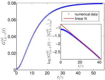
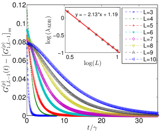
Figure 1: (Color online) (Top) Runge-Kutta time evolution of the pairing correlator $G^{(p)}_{1,L-1}(t)$ for the largest available system size, $L=10$. The inset shows that upon subtraction of the steady value, an exponential decay is observed, from which $\lambda_{\rm ADR}$ is extracted. (Bottom) Time evolution of $G^{(p)}_{1,L-1}(t)-\big{[}G^{(p)}_{1,L-1}\big{]}_{\rm ss}$ for several system sizes. The inset shows the scaling of $\lambda_{\rm ADR}$ with $L$, which is fitted by an algebraic function.

Let us first assess that the asymptotic decay rate of the system closes polynomially with the system size (from the previous analysis we know that it closes at least polynomially. As we discuss in Appendix A, in the asymptotic limit, it is possible to represent the expectation value of any observable $\hat{A}$ as:

$$\langle\hat{A}\rangle(t)-\langle\hat{A}\rangle_{\rm ss}\sim\kappa e^{-\lambda_{\rm ADR}t}+\ldots$$ (24)

where $\langle\hat{A}\rangle(t)={\rm tr}\big{[}\hat{A}\,\hat{\rho}(t)\big{]}$, $\langle\hat{A}\rangle_{\rm ss}=\lim_{t\to\infty}\langle\hat{A}\rangle(t)$ and $\kappa$ is a non-universal constant. The notation $-\lambda_{\rm ADR}$ is due to the fact that $\lambda_{\rm ADR}$ is positive, being defined through the additive inverse of the real part of the eigenvalues, see Eq. (4). It is possible to envision situations where $\kappa=0$ and thus the long-time decay is dominated by eigenvalues of $\mathcal{L}^{\prime}$ with smaller real part.

The study of the long-time dependence of any observable can be used to extract the value of $\lambda_{\rm ADR}$; among all the possible choices, we employ the pairing correlator $G^{(p)}_{j,l}(t)=\langle\hat{O}_{j}^{(p)\dagger}\hat{O}^{(p)}_{l}\rangle(t)$ [see Eq. (20)] because of its special physical significance. In Fig. 1(top), we consider $L=10$ and plot the time evolution of $G^{(p)}_{j,l}(t)$ for $j=1$ and $l=L-1$ (no relevant boundary effects have been observed as far as the estimation of $\lambda_{\rm ADR}$ is concerned). The calculation is performed through RK integration of the master equation. The initial state of the evolution is given by the ground state of the non-interacting Hamiltonian, $\hat{\mathcal{H}}_{0}=-J\sum_{j}\hat{a}^{\dagger}_{j}\hat{a}_{j+1}+{\rm H.c.}$ ($N=L/2$ for $L$ even, and $N=(L+1)/2$ for $L$ odd).

In order to benchmark the reliability of the RK integration for getting the steady state, we compare the expectation value of several observables (in particular of pairing correlators) with the exactly-known results (Sec. III provides the exact wavefunction of the steady state, from which several observables can be computed). In all cases the absolute differences are below $10^{-6}$. Similar results are obtained for smaller system sizes, where it is even possible to compute the trace-distance of the RK steady-state from the $\lambda=0$ eigenstate of the Liouvillian computed with ED.

In the long-time limit, the observable (20) displays a clear stationary behavior, $\big{[}G^{(p)}_{j,l}\big{]}_{\rm ss}=\lim_{\tau\to\infty}G^{(p)}_{j,l}(\tau)$, consistently with Eq. (24). Once such stationary value is subtracted, it is possible to fit $\lambda_{\rm ADR}$ from the exponential decay of

$$G^{(p)}_{j,l}(t)-\big{[}G^{(p)}_{j,l}\big{]}_{\rm ss}$$ (25)

The subtraction is possible to high precision because the value of $\big{[}G^{(p)}_{j,l}\big{]}_{\rm ss}$ is known from the previous analytical considerations. Moreover, as we have already pointed out, the evolution continues up to times such that $G^{(p)}_{j,l}(t)$ differs in absolute terms from the analytical value for $\lesssim 10^{-6}$, which makes the whole procedure reliable.

In Fig. 1(bottom) we display the quantity in (25) for various lattice sizes $L$. It is clear that the convergence of the observable requires an amount of time which increases with $L$. A systematic fit of $\lambda_{\rm ADR}$ for several chain lengths allows for an estimate of its dependence on $L$ [see Fig. 1(bottom)]: the finite-size dissipative gap scales as

$$\lambda_{\rm ADR}\propto L^{-2.13\pm 0.05}\;.$$ (26)

The exact diagonalization (ED) of the Liouvillian up to $L=5$ allows a number of further considerations. First, the Liouvillian eigenvalues with largest real part ($\Re(\lambda)\lesssim 0$) are independent of the number of particles (the check has been performed for every value of $N=1,...,5$). Second, comparing the ED with the previous analysis, we observe that the $\lambda_{\rm ADR}$ in Eq. (26) coincides with the second eigenvalue of the Liouvillian, rather than with the first [here the generalized eigenvalues are ordered according to the additive inverse of their real part $-\Re(\lambda)$]. Numerical inspection of small systems (up to $L=5$) shows that the first excited eigenvalue of $\mathcal{L}^{\prime}$ is two-fold degenerate and takes the value $-\xi/2$, where $\xi$ is the energy of the first excited state of $\hat{\mathcal{H}}^{\prime}_{p}$ (see the discussion in Sec. II.1). Our numerics suggests that it does not play any role in this particular dissipative evolution, hinting at the fact that the chosen $\hat{\rho}(0)$ does not overlap with the eigensubspace relative to $-\xi/2$. In this case, the value of $\kappa$ in Eq. (24) is zero.

IV.2 Perturbations

In order to test the robustness of the dissipative scheme for the preparation of a p-wave superconductor, we now consider several perturbations of the Lindbladian $\mathcal{L}^{\prime}$ of both dissipative and Hamiltonian form. The robustness of the dissipative state preparation of the p-wave superconductor is probed through the behavior of the correlations $G^{(p)}_{j,l}(t)$, which define such phase.

IV.2.1 Perturbations of the Lindblad operators

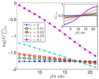
Figure 2: (Color online) Steady-state values of $\big{[}G^{\prime(p)}_{4,j}\big{]}_{\rm ss}$ [see Eq. (28)] for a lattice with $L=22$ sites at half-filling, $\nu=1/2$, computed with MPDO for different values of $\epsilon$ in $\hat{L}^{\prime}_{j,\epsilon}$ [see Eq. (27)]. The inset displays the steady-state values of the local number of fermions $\langle\hat{n}_{j}\rangle_{\rm ss}$ for the same systems.

Let us define the following perturbed Lindblad operator:

$$\hat{L}^{\prime}_{j,\epsilon}=\hat{C}_{j}^{\dagger}\hat{A}_{j,\epsilon};\quad\hat{A}_{j,\epsilon}=\hat{a}_{j}-(1-\epsilon)\hat{a}_{j+1};\quad\epsilon\in\mathbb{R},$$ (27)

which allows for slight asymmetries in the action of the dissipation between sites $j$ and $j+1$. The continuity equation associated to the dynamics, $\partial_{t}\hat{n}_{i}=-(\hat{j}_{i}-\hat{j}_{i-1})$, is characterized by the following current operator: $\hat{j}_{i}=\hat{n}_{i}-(1-\epsilon)^{2}\hat{n}_{j}+(\epsilon^{2}-2\epsilon)\hat{n}_{i}\hat{n}_{i+1}$. When $\epsilon\neq 0$, $\hat{j}_{i}$ is not anymore odd under space reflection around the link between sites $i$ and $i+1$, so that in the stationary state a non-zero current can flow even if the density profile is homogeneous (and even under the previous space-inversion transformation), which is quite intuitive given the explicit breaking of inversion symmetry in this problem.

We employ the MPDO method to analyze the steady-state properties of a system with size $L=22$ initialized in the ground state of the free Hamiltonian $\hat{\mathcal{H}}_{0}$ for $N=11$ and subject to such dissipation. The results in the inset of Fig. 2 show that the steady state is not homogeneous and that a relatively high degree of inhomogeneity $\frac{\langle\hat{n}_{L}\rangle-\langle\hat{n}_{1}\rangle}{\langle\hat{n}_{L/2}\rangle}\approx 1$ is found also for small perturbations $\epsilon=0.05$. This is not to be confused with the phase-separation instability which characterizes the ferromagnetic parent Hamiltonian $\hat{\mathcal{H}}^{\prime}_{p,\mathrm{spin}}$. Indeed, if PBC are considered, the system becomes homogeneous and a current starts flowing in it (not shown here).

P-wave superconducting correlations are affected by such inhomogeneity. Whereas for $\epsilon=0$ the correlations $\big{[}G^{(p)}_{j,l}\big{]}_{\rm ss}$ do not show a significant dependence on $|j-l|$, this is not true even for small perturbations $\epsilon\leq 0.05$. In order to remove the effect of the inhomogeneous density, in Fig. 2 we show the value of properly rescaled p-wave correlations:

$$\big{[}G^{\prime(p)}_{j,l}\big{]}_{\rm ss}\equiv\langle\,\hat{O}^{\prime(p)\dagger}_{j}\,\hat{O}^{\prime(p)}_{l}\,\rangle_{\rm ss}=\frac{(N/L)^{4}\,\langle\hat{O}^{(p)\dagger}_{j}\hat{O}^{(p)}_{l}\rangle_{\rm ss}}{\langle\hat{n}_{j}\rangle_{\rm ss}\langle\hat{n}_{j+1}\rangle_{\rm ss}\langle\hat{n}_{l}\rangle_{\rm ss}\langle\hat{n}_{l+1}\rangle_{\rm ss}}$$ (28)

where $\hat{O}^{\prime(p)}_{j}=(N/L)^{2}\hat{O}^{(p)}_{j}/(\langle\hat{n}_{j}\rangle_{\rm ss}\langle\hat{n}_{j+1}\rangle_{\rm ss})$. An exponential decay behavior appears as a function of $|j-l|$, which becomes more pronounced when $\epsilon$ is increased. Even if the simulation is performed on a finite short system, for significant perturbations, $\epsilon=0.1$, the value of $\big{[}G^{\prime(p)}_{j,l}\big{]}_{\rm ss}$ decays of almost two decades, so that the exponential behavior is identified with reasonable certainty.

In Appendix B we discuss some interesting analogies of these results with the properties of the ground state of the parent Hamiltonian $\hat{\mathcal{H}}^{\prime}_{p,\epsilon}=J\sum_{j}\hat{L}_{j,\epsilon}^{\prime\dagger}\hat{L}^{\prime}_{j,\epsilon}$. It should be stressed that, since $\hat{\mathcal{H}}^{\prime}_{p,\epsilon}$ does not have a zero-energy ground state, there is no exact correspondence between its ground state and the steady states of $\mathcal{L}_{\epsilon}^{\prime}$.

Concluding, we mention that a similar analysis can be done introducing an analogous perturbation in the operator $\hat{C}_{j}^{\dagger}$; our study did not observe any qualitative difference (not shown).

IV.2.2 Perturbations due to unitary dynamics

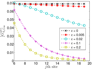
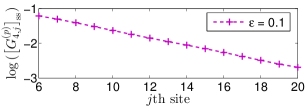
Figure 3: (Color online) (Top) Pairing correlations $\big{[}G^{(p)}_{4,j}\big{]}_{\rm ss}$ for the steady state of the dynamics in the presence of a Hamiltonian perturbation (29). The calculation of the steady state is performed with MPDO technique for $L=22$ and $N=11$. (Bottom) The decay of $\big{[}G^{(p)}_{4,j}\big{]}_{\rm ss}$ is exponential in $j$ (here, $\epsilon=0.1$).

An alternative way of perturbing the dynamics of $\mathcal{L}^{\prime}$ in Eq. (14) is to introduce a Hamiltonian into the system, chosen for simplicity to be the already-introduced free Hamiltonian $\hat{\mathcal{H}}_{0}$:

$$\frac{\partial}{\partial t}\hat{\rho}=-i[\epsilon\hat{\mathcal{H}}_{0},\hat{\rho}]+\mathcal{L}[\hat{\rho}].$$ (29)

Using the MPDO method to characterize the steady state of the dynamics, we analyze the spatial decay of the pairing correlations for $L=22$ and at half-filling ($N=11$); the initial state is set in the same way as in the previous section. In Fig. 3 (top) we display the results: even for very small perturbations the pairing correlator $\big{[}G^{(p)}_{4,j}\big{]}_{\rm ss}$ decays rapidly in space. The long-distance saturation observed in the absence of perturbations is lost and qualitatively different from this result. In Fig. 3 (bottom) we highlight that the decay is exponential.

Summarizing, in all the cases that we have considered, the p-wave pairing correlations of the stationary state $\big{[}G^{(p)}_{j,l}\big{]}_{\rm ss}$ are observed to decay as a function of $|j-l|$. Due to the interplay between the targeted dissipative dynamics and the perturbations, which do not support a p-wave ordered dark state, the steady state is mixed, similar to a finite temperature state. From this intuition, the result is easily rationalized: Any (quasi) long range order is destroyed in one-dimensional systems at finite temperature. We note that the true long range order found in the unperturbed case (correlators saturating at large distance; opposed to the more generic quasi-long range order defined with algebraic decay) is non-generic in one-dimensional systems and a special feature of our model, see Iemini_2015 for a thorough discussion. However, the destruction of any such order via effective finite temperature effects must be expected on general grounds. The absence of quasi-long-range p-wave superconducting order, which in one-dimension only occurs at zero-temperature for pure state, is likely to be in connection with this fact.

IV.2.3 Perturbation strength

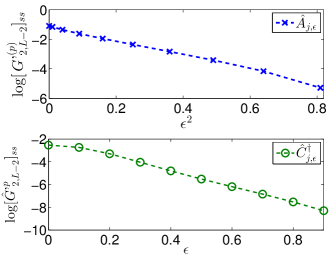
Figure 4: (Color online) $\big{[}G^{\prime(p)}_{2,L-2}\big{]}_{\rm ss}$ in the presence of a perturbed Lindblad operator as a function of the perturbation strength $\epsilon$. The perturbation is considered both for the $\hat{A}_{j}$ (top) and $\hat{C}^{\dagger}_{j}$ (bottom) operators (see text for the definitions). The calculation is done with RK integration of the equation of motion for $L=8$ and $N=4$.

Finally, we perform a quantitative investigation of the dependence of the pairing correlations on the perturbation strength, $\epsilon$.

Lindblad perturbation – In Fig. 4 we plot the p-wave superconducting correlation $\big{[}G^{(p)}_{2,L-2}\big{]}_{\rm ss}$ of a system of length $L=8$ as a function of the intensity of the perturbation $\epsilon$ in $\hat{L}^{\prime}_{j,\epsilon}$ (for completeness, the complementary case $\hat{L}^{\prime(2)}_{j,\epsilon}=\hat{C}_{j,\epsilon}^{\dagger}\hat{A}_{j}$, with $\hat{C}_{j,\epsilon}^{\dagger}=\hat{a}_{j}^{\dagger}+(1-\epsilon)\hat{a}^{\dagger}_{j+1}$, is also included). Our data confirm that correlations undergo a clear suppression in the presence of $\epsilon\neq 0$, which in one case is exponential in $\epsilon$ and in the other in $\epsilon^{2}$. The calculation is performed through RK integration of the dynamics.

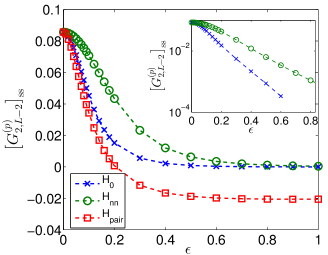
Figure 5: (Color online) $\big{[}G^{(p)}_{2,L-2}\big{]}_{\rm ss}$ in the presence of a perturbing Hamiltonian as a function of the perturbation strength $\epsilon$. We consider $\hat{\mathcal{H}}_{0}$, $\hat{\mathcal{H}}_{\rm nn}$ and $\hat{\mathcal{H}}_{\rm pair}$ (see text for the definitions). The inset highlights the exponential decay with $\epsilon$.

Hamiltonian perturbation – We begin with the two cases: $\hat{\mathcal{H}}_{0}$ and $\hat{\mathcal{H}}_{\rm nn}=-J\sum_{j}\hat{n}_{j}\hat{n}_{j+1}$. Fig. 5 shows, in both cases, an exponential decay to zero of $\big{[}G^{\prime(p)}_{2,L-2}\big{]}_{\rm ss}$ when $\epsilon$ is increased. On the contrary, a Hamiltonian which introduces p-wave correlations in the system, such as

$$\hat{\mathcal{H}}_{\rm pair}=-J\sum_{j,l}(\hat{a}^{\dagger}_{j}\hat{a}^{\dagger}_{j+1}\hat{a}_{l+1}\hat{a}_{l}+{\rm H.c.}),$$ (30)

changes the value and the sign of $\big{[}G^{\prime(p)}_{2,L-2}\big{]}_{\rm ss}$, leaving it different from zero.

Concluding, we have shown that in all the considered cases, perturbations of both dissipative and Hamiltonian form are detrimental to the creation of a p-wave superconductor. This is rationalized by the mixedness of the stationary state in that case, and parallels a finite temperature situation. In any generic, algebraically ordered system at T=0, one has gapless modes.

V Two wires

An intuitive explanation of why the dissipative setup discussed in Sec. III does not show topological dark states with fixed number of particles is the fact that this constraint fixes the parity of the state, and thus no topological degeneracy can occur. It has already been realized in several works that a setup with two parallel wires can overcome this issue Fidkowski_2011 ; Sau_2011 ; Cheng_2011 ; Kraus_2013 ; Ortiz_2014 ; Iemini_2015 ; Lang_2015 . In this case it is possible to envision a number-conserving p-wave superconducting Hamiltonian which conserves the parity of the number of fermions in each wire: such symmetry can play the role of the parity of the number of fermions for $\hat{\mathcal{H}}_{\rm K}$ in Eq. (8). Several equilibrium models have already been discussed in this context; here we consider the novel possibility of engineering a topological number-conserving p-wave superconductor with Markovian dynamics.

V.1 Steady states

Let us study a system composed of two wires with spinless fermions described by the canonical fermionic operators $\hat{a}_{j}^{(\dagger)}$ and $\hat{b}_{j}^{(\dagger)}$. For this model we consider three kinds of Lindblad operators:

$$\hat{L}^{\prime\prime}_{a,j}=\hat{C}_{a,j}^{\dagger}\hat{A}_{a,j};$$ (31a)

$$\hat{L}^{\prime\prime}_{b,j}=\hat{C}_{b,j}^{\dagger}\hat{A}_{b,j};$$ (31b)

$$\hat{L}^{\prime\prime}_{I,j}=\hat{C}_{a,j}^{\dagger}\hat{A}_{b,j}+\hat{C}^{\dagger}_{b,j}\hat{A}_{a,j}.$$ (31c)

We now characterize the dark states of the Markovian dynamics induced by these operators for a two-leg ladder of length $L$ with hard-wall boundary conditions:

$$\frac{\partial}{\partial t}\hat{\rho}=\mathcal{L}^{\prime\prime}[\hat{\rho}]=\gamma\sum_{j=1}^{L-1}\sum_{\Lambda=a,b,I}\left[\hat{L}_{\Lambda,j}^{\prime\prime}\hat{\rho}\hat{L}_{\Lambda,j}^{\prime\prime\dagger}-\frac{1}{2}\{\hat{L}_{\Lambda,j}^{\prime\prime\dagger}\hat{L}^{\prime\prime}_{\Lambda,j},\hat{\rho}\}\right].$$ (32)

In particular, we will show that, for every fermionic density different from the completely empty and filled cases, there are always two steady states.

It is easy to identify the linear space $\mathcal{S}_{N}$ of states which are annihilated by the $\hat{L}^{\prime\prime}_{a,j}$ and $\hat{L}^{\prime\prime}_{b,j}$ and have a total number of particles $N$:

$$\mathcal{S}_{N}=\text{span}\{|\psi_{a,0}\rangle|\psi_{b,N}\rangle,|\psi_{a,1}\rangle|\psi_{b,N-1}\rangle,\ldots,|\psi_{a,N}\rangle|\psi_{b,0}\rangle\}.$$ (33)

where the states $|\psi_{\alpha,N}\rangle$ are those defined in Eq. (17) for the wire $\alpha=a,b$. Let us consider a generic state in $\mathcal{S}_{N}$:

$$|\psi\rangle=\sum_{m=0}^{N}\alpha_{m}|\psi_{a,m}\rangle|\psi_{b,N-m}\rangle,\quad\sum_{m=0}^{N}|\alpha_{m}|^{2}=1.$$ (34)

From the condition $\hat{C}^{\dagger}_{j}|\psi_{\sigma}\rangle=-\hat{A}_{j}|\psi_{\sigma}\rangle$ we obtain:

$$\hat{C}^{\dagger}_{j}|\psi_{N-1}\rangle =-\hat{A}_{j}|\psi_{N+1}\rangle,\quad N\in(0,2L)$$ (35a)

$$0 =-\hat{A}_{j}|\psi_{1}\rangle,$$ (35b)

$$\hat{C}^{\dagger}_{j}|\psi_{2L-1}\rangle =0,$$ (35c)

and when we impose the condition $\hat{L}^{\prime\prime}_{I,j}|\psi\rangle=0$:

$$\hat{L}^{\prime\prime}_{I,j}|\psi\rangle= \sum_{m=0}^{N-1}\alpha_{m}\hat{C}^{\dagger}_{a,j}\hat{A}_{b,j}|\psi_{a,m}\rangle|\psi_{b,N-m}\rangle+\sum_{m=1}^{N}\alpha_{m}\hat{C}^{\dagger}_{b,j}\hat{A}_{a,j}|\psi_{a,m}\rangle|\psi_{b,N-m}\rangle=$$

$$= \sum_{m=0}^{N-1}\alpha_{m}\hat{C}^{\dagger}_{a,j}\hat{A}_{b,j}|\psi_{a,m}\rangle|\psi_{b,N-m}\rangle-\sum_{m=2}^{N+1}\alpha_{m}\hat{C}^{\dagger}_{a,j}\hat{A}_{b,j}|\psi_{a,m-2}\rangle|\psi_{b,N-m+2}\rangle=0.$$ (36)

The result is $\alpha_{m}=\alpha_{m+2}$, so that two linearly independent states can be constructed which are annihilated by all the Lindblad operators in (31):

$$|\psi_{N,ee}\rangle= \frac{1}{\mathcal{N}_{N,ee}^{1/2}}\sum_{m}|\psi_{a,2m}\rangle|\psi_{b,N-2m}\rangle,$$ (37a)

$$|\psi_{N,oo}\rangle= \frac{1}{\mathcal{N}_{N,oo}^{1/2}}\sum_{m}|\psi_{a,2m-1}\rangle|\psi_{b,N-2m+1}\rangle.$$ (37b)

The subscripts $ee$ and $oo$ refer to the fermionic parities in the first and second wire assuming that $N$ is even; $\mathcal{N}_{N,ee}$ and $\mathcal{N}_{N,oo}$ are normalization constants Iemini_2015 . For $N$ odd one can similarly construct the states $|\psi_{N,eo}\rangle$ and $|\psi_{N,oe}\rangle$. By construction, the states that we have just identified are the only dark states of the dynamics.

It is an interesting fact that at least two parent Hamiltonians are known for the states in (37), as discussed in Refs. Iemini_2015 ; Lang_2015 . We refer the reader interested in the full characterization of the topological properties of these steady-states to those articles.

Finally, let us mention that the form of the Lindblad operators in (31) is not uniquely defined. For example one could replace $\hat{L}^{\prime\prime}_{I,j}$ in Eq. (31c) with the following:

$$\hat{L}^{\prime\prime}_{I,j}=\left(\hat{C}_{a,j}^{\dagger}+\hat{C}_{b,j}^{\dagger}\right)\left(\hat{A}_{a,j}+\hat{A}_{b,j}\right),$$ (38)

without affecting the results Iemini_2015 . The latter operator is most realistic for an experimental implementation, as we point out below.

V.2 P-wave superconductivity

Let us now check that the obtained states are p-wave superconductors. Similarly to the single-wire protocol discussed in Eq. (21), the explicit calculation Iemini_2015 shows that p-wave correlations saturate to a final value at large distances in the thermodynamic limit [for the two-leg ladder we consider $\nu=N/(2L)$]

$$\langle\psi_{N,ee}|\hat{O}_{j}^{(p)\dagger}\hat{O}^{(p)}_{l}|\psi_{N,ee}\rangle\xrightarrow{|j-l|\rightarrow\infty}\nu^{2}(1-\nu)^{2}.$$ (39)

This relation clearly highlights the p-wave superconducting nature of the states.

V.3 Dissipative gap

In order to demonstrate that the asymptotic decay rate $\lambda_{\rm ADR}$ associated to $\mathcal{L}^{\prime\prime}$ tends to $0$ in the thermodynamic limit, we consider the parent Hamiltonian of the model:

$$\hat{\mathcal{H}}_{p}^{\prime\prime}\!=\! -4J\!\!\sum_{\begin{subarray}{c}j=1\\ \alpha=a,b\end{subarray}}^{L-1}\!\!\Big{[}(\hat{\alpha}^{\dagger}_{j}\hat{\alpha}_{j+1}\!+\!\text{H.c.})-\!(\hat{n}_{j}^{\alpha}+\hat{n}_{j+1}^{\alpha})+\!\hat{n}_{j}^{\alpha}\hat{n}_{j+1}^{\alpha}\Big{]}$$

$$-2J\sum_{j=1}^{L-1}\Big{[}(\hat{n}_{j}^{a}+\hat{n}_{j+1}^{a})(\hat{n}_{j}^{b}+\hat{n}_{j+1}^{b})-(\hat{a}^{\dagger}_{j}\hat{a}_{j+1}\hat{b}^{\dagger}_{j}\hat{b}_{j+1}$$

$$\hskip 18.49411pt+\hat{a}_{j}^{\dagger}\hat{a}_{j+1}\hat{b}^{\dagger}_{j+1}\hat{b}_{j}-2\hat{b}^{\dagger}_{j}\hat{b}^{\dagger}_{j+1}\hat{a}_{j+1}\hat{a}_{j}+{\rm H.c.})\Big{]},$$ (40)

where $J>0$ is a typical energy scale setting the units of measurement. This Hamiltonian has been extensively analyzed in Ref. Iemini_2015 . Numerical simulations performed with the density-matrix renormalization-group algorithm assess that $\hat{\mathcal{H}}_{p}^{\prime\prime}$ is gapless and that the gap is closing as $1/L^{2}$. According to the discussion in Sec. II.1, the asymptotic decay rate $\lambda_{\rm ADR}$ associated to the Lindbladian $\mathcal{L}^{\prime\prime}$ closes in the thermodynamic limit with a scaling which is equal to $\sim L^{-2}$ or faster. This is true both for periodic and hard-wall boundary conditions.

V.4 Experimental implementation

The Lindblad operators in Eqs. (31a), (31b) and (38) lend themselves to a natural experimental implementation. The engineering of terms like $\hat{L}^{\prime\prime}_{a,j}$ and $\hat{L}^{\prime\prime}_{b,j}$ has been extensively discussed in Ref. Diehl_2011 starting from ideas originally presented in Ref. Diehl_2008 . As we will see, the Lindblad operator $\hat{L}^{\prime\prime}_{I,j}$ in Eq. (38) is just a simple generalization.

The idea is as follows: a superlattice is imposed which introduces in the system additional higher-energy auxiliary sites located in the middle of each square of the lower sites target lattice. Driving lasers are then applied to the system, whose phases are chosen such that the excitation to the auxiliary sites happens only for states $|\varphi\rangle$ such that $(\hat{A}_{a,j}+\hat{A}_{b,j})|\varphi\rangle\neq 0$. If the whole system is immersed into, e.g., a Bose-Einstein condensate reservoir, atoms located in the auxiliary sites can decay to the original wire by emission of a Bogoliubov phonon of the condensate. This process is isotropic and, for a wavelength of the emitted phonons comparable to the lattice spacing, gives rise to the four-site creation part with relative plus sign: $\hat{C}^{\dagger}_{a,j}+\hat{C}^{\dagger}_{b,j}$.

V.5 Perturbations

An important property of topological Hamiltonians is the robustness of their edge physics to local perturbations. Similar features have been highlighted in the case of topological superconductors where the setup is not number conserving Diehl_2011 ; Bardyn_2013 . The goal of this section is to probe the resilience of the twofold-degenerate steady states of $\mathcal{L}^{\prime\prime}$. A conclusive analysis is beyond our current numerical possibilities; here we present some preliminary results obtained via exact diagonalization methods.

We consider the natural choice of Lindblad operators Eqs. (31a,31b,38), subject to perturbations:

$$\hat{L}^{\prime\prime}_{a,j,\epsilon}=\hat{C}_{a,j}^{\dagger}\hat{A}_{a,j,\epsilon};\quad\hat{A}_{a,j,\epsilon}=\hat{a}_{j}-(1-\epsilon)\hat{a}_{j+1};$$ (41a)

$$\hat{L}^{\prime\prime}_{b,j,\epsilon}=\hat{C}_{b,j}^{\dagger}\hat{A}_{b,j,\epsilon};\quad\hat{A}_{b,j,\epsilon}=\hat{b}_{j}-(1-\epsilon)\hat{b}_{j+1};$$ (41b)

$$\hat{L}^{\prime\prime}_{I,j}=\left(\hat{C}_{a,j}^{\dagger}+\hat{C}_{b,j}^{\dagger}\right)\left(\hat{A}_{a,j,\epsilon}+\hat{A}_{b,j,\epsilon}\right);\quad\epsilon\in\mathbb{R}$$ (41c)

Those define a perturbed Lindbladian $\mathcal{L}^{\prime\prime}_{\epsilon}$. They are a simple generalization of those defined in Eq. (27) for the single-wire setup.

Let us begin our analysis by showing that for small sizes $L\sim 6$ the degeneracy of the steady space for $\epsilon=0$ is broken. Let us first remark that for $\epsilon=0$ the steady space is four-fold degenerate; a possible parameterization is:

$$\mathcal{B}=\{ |\psi_{N,ee}\rangle\langle\psi_{N,ee}|,\quad|\psi_{N,ee}\rangle\langle\psi_{N,oo}|,$$ (42)

$$|\psi_{N,oo}\rangle\langle\psi_{N,ee}|,\quad|\psi_{N,oo}\rangle\langle\psi_{N,oo}|\}.$$ (43)

A direct inspection of the eigenvalues of $\mathcal{L}_{\epsilon}$ shows that this degeneracy is broken once $\epsilon\neq 0$. Results, shown in Fig. 6 for a fixed lattice size $L=6$ and $N=6$, display a quadratic splitting of the steady steady degeneracy with the perturbation strength.

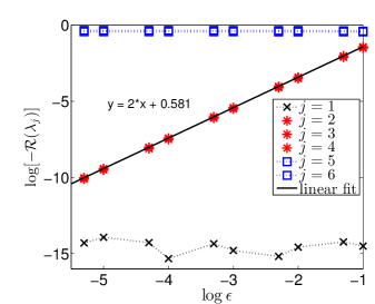
Figure 6: (Color online) Real part of the first six eigenvalues of the Lindbladian operator $\mathcal{L}^{\prime\prime}_{\epsilon}$ for $L=6$ and $N=6$ as a function of $\epsilon$. Eigenvalues $\lambda_{j}$ are sorted according to increasing $-\Re(\lambda_{j})$. The plot highlights the presence of a $\lambda=0$ eigenvalue (within numerical accuracy $10^{-15}$), of three eigenvalues which scale as $\epsilon^{2}$ and of other eigenvalues of magnitude $\sim 1$.

Let us now check the behavior with the system size of the first eigenvalues of the system for longer system sizes. In order to obtain a reasonable number of data, the extreme choice of setting $N=2$ in all simulations has been taken, which allows us to analyze system sizes up to $L=20$. Results shown in Fig. 7 (top) show that the Liouvillian eigenvalues related to the steady-state degeneracy display an algebraic scaling $\lambda_{\rm ADR}\sim L^{-1}$ in the accessible regime of system sizes for small perturbations ($\epsilon=10^{-2}$), while they are gapped for larger perturbations ($\epsilon=10^{-1}$). Note that, for the system sizes which could be accessed, larger eigenvalues clear display an algebraic decay, as shown in Fig. 7 (bottom), also for $\epsilon=0.1$. The scaling of the eigenvalues related to the steady state degeneracy is not exponential and thus in principle should not be connected to the topological properties of the system. However, these preliminary considerations suffer from two significant biases: (i) the small considered sizes, (ii) the fact that they are not performed at exactly fixed density, and (iii) the very low filling. A more thorough analysis is left for future work.

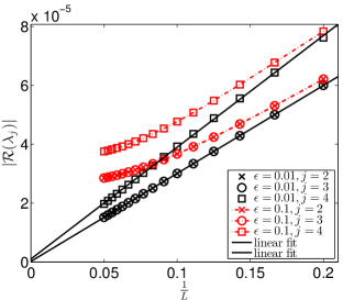
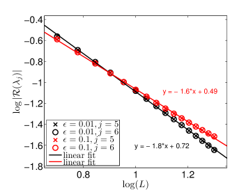
Figure 7: (Color online) Real part of the eigenvalues $j=2$, $3$ and $4$ (top) and $j=5$ and $6$ (bottom) of the Lindbladian operator $\mathcal{L}^{\prime\prime}_{\epsilon}$ for $N=2$ as a function of $L$ (here, $L\leq 20$). The two values $\epsilon=0.1$ and $\epsilon=0.01$ are considered. In the top panel, the values of the eigenvalues relative to $\epsilon=0.1$ have been rescaled by $0.01$ in order to facilitate the readability of the plot.

VI Conclusions

In this article we have discussed the dissipative quantum state preparation of a p-wave superconductor in one-dimensional fermionic systems with fixed number of particles. In particular, we have presented two protocols which have been fully characterized in the presence of hard-wall boundaries. Whereas the former does not display topological property, the latter features a two-dimensional steady space to be understood in terms of boundary Majorana modes for any number of fermions. Through the analysis of a related parent Hamiltonian, we are able to make precise statements about the gapless nature of the Lindbladian super-operators associated to both dynamics.

The peculiar form of the master equations considered in this article allows for the exact characterization of several properties of the system, and in particular of the steady state, even if the dynamics is not solvable with the methods of fermionic linear optics Prosen_2008 ; Bravyi_2012 exploited in Refs. Diehl_2011 ; Bardyn_2013 . This result is very interesting per se, as such examples are usually rare but can drive physical intuition into regimes inaccessible without approximations. It is a remarkable challenge to investigate which of the properties presented so far are general and survive to modifications of the environment, and which ones are peculiar of this setup.

Using several numerical methods for the study of dissipative many-body systems, we have presented a detailed analysis of the robustness to perturbations of these setups. Through the calculation of the proper p-wave correlations we have discussed how external perturbations can modify the nature of the steady state. In the ladder setup, where the steady states are topological, we have presented preliminary results on the stability of the degenerate steady-space of the system.

The analysis presented here has greatly benefited from exact mathematical relations between the properties of the Lindbladian and of a related parent Hamiltonian. Since the study of closed systems is much more developed than that of open systems both from the analytical and from the numerical points of view, a more detailed understanding of the relations between Lindbladians and associated parent Hamiltonian operators stands as a priority research program.

Appendix A Spectral properties of the Lindbladian super-operator

In order to discuss the long-time properties of the dissipative dynamics, it is convenient to start from the spectral decomposition of the Lindbladian. Since $\mathcal{L}$ is in general a non-Hermitian operator, its eigenvalues are related to its Jordan canonical form Kato . Let us briefly review these results. The Hilbert space of linear operators on the fermionic Fock space, $\mathbb{H}$, can be decomposed into the direct sum of linear spaces $\mathbb{M}_{j}$ (usually not orthogonal) such that if we denote with $\mathcal{P}_{j}$ the projectors onto such subspaces (usually not orthogonal) and with $\mathcal{N}_{j}$ a nilpotent super-operator acting on $\mathbb{M}_{j}$, the following is true:

$$\mathcal{L}=\sum_{j}\left[\lambda_{j}\mathcal{P}_{j}+\mathcal{N}_{j}\right].$$ (44)

The $\{\lambda_{j}\}$ are the generalized complex eigenvalues of the super-operator ${\mathcal{L}}$ and, for the case of a Lindbladian, have non-positive real part; the $\mathcal{N}_{j}$ can also be equal to zero. By this explicit construction it is possible to observe that the $\{\mathcal{P}_{j}\}$ and $\{\mathcal{N}_{j}\}$ are all mutually commuting ($\mathcal{P}_{j}\mathcal{P}_{k}=\delta_{j,k}\mathcal{P}_{j}$, $\mathcal{P}_{j}\mathcal{N}_{k}=\mathcal{N}_{k}\mathcal{P}_{j}=\delta_{j,k}\mathcal{N}_{j}$ and $\mathcal{N}_{j}\mathcal{N}_{k}=\delta_{j,k}\mathcal{N}_{j}^{2}$).

Using these properties, the time evolution can be written as:

$$\hat{\rho}(t)=e^{t\mathcal{L^{\prime}}}[\hat{\rho}(0)]=\sum_{j}e^{\lambda_{j}t}e^{t\mathcal{N}_{j}}\mathcal{P}_{j}[\hat{\rho}(0)],$$ (45)

which highlights that at a given time $t$ only the terms of the sum such that $|\Re(\lambda_{j})\,t|\ll 1$ play a role. In the long-time limit, it is possible to represent the expectation value of any observable $\hat{A}$ as:

$$\langle\hat{A}\rangle(t)\approx\text{tr}[\hat{A}\,\mathcal{P}_{0}[\hat{\rho}(0)]]+\,e^{-\lambda_{\rm ADR}t}\,\text{tr}[\hat{A}\,e^{t\mathcal{N}_{\rm ADR}}\mathcal{P}_{\rm ADR}[\hat{\rho}(0)]].$$ (46)

Eq. (46) is the mathematical formula motivating Eq. (24) in the text, defining also the meaning of $\kappa$.

Let us mention that in the example discussed in the text $\mathcal{N}_{\rm ADR}=0$: this is observed by explicit inspection via exact diagonalization of small systems ($L=5$). Since the presence of a non-zero nilpotent super-operator is a fine-tuned property, it is reasonable to assume that the situation remains similar for longer systems.

Appendix B Analogies with the parent Hamiltonian

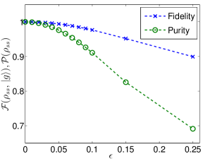
Figure 8: (Color online) Fidelity $\mathcal{F}(\rho_{ss},|g\rangle)$ and purity $\mathcal{P}(\rho_{ss})$ for different values of $\epsilon$ in $\hat{L}^{\prime}_{j,\epsilon}$ [see Eq. (27)].

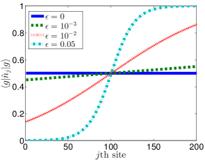
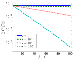
Figure 9: (Color online) (top) Density profile $\langle g|\hat{n}_{j}|g\rangle$ and (bottom) renormalized pairing correlations $\langle g|\hat{O}^{\prime(p)\dagger}_{j}\hat{O}^{\prime(p)}_{\ell}|g\rangle$, with $j=(L/2)-2$ and $\ell>j$. The computation is performed for a lattice with $L=200$ sites at half-filling and different values of $\epsilon$ in $\hat{L}^{\prime}_{j,\epsilon}$ [see Eq. (27)].

In this Appendix we discuss some interesting analogies between the steady state $\hat{\rho}_{\rm ss}$ of the dissipative dynamics for the perturbed Lindblad operator $\hat{L}^{\prime}_{j,\epsilon}$ in Eq. (27) with the ground state $|g\rangle$ of its parent Hamiltonian $\hat{\mathcal{H}}^{\prime}_{p,\epsilon}=J\sum_{j}\hat{L}_{j,\epsilon}^{\prime\dagger}\hat{L}^{\prime}_{j,\epsilon}$. It should be stressed that, since $\hat{\mathcal{H}}^{\prime}_{p,\epsilon}$ does not have a zero-energy ground state, there is no exact correspondence between both states.

We first study a small lattice with $L=8$ sites at half-filling, performing a Runge-Kutta integration of the master equation. The initial state of the evolution is the ground state of $\hat{\mathcal{H}}_{0}$. In Fig. 8 it is shown that both the purity of the steady state $\mathcal{P}(\rho_{ss})={\rm tr}\big{[}\hat{\rho}_{ss}^{2}\big{]}$ and its fidelity with the ground state of the parent Hamiltonian decrease with the perturbation strength. Notice, however, that for small perturbations the fidelity $\mathcal{F}(\hat{\rho}_{\rm ss},|g\rangle)=\langle g|\hat{\rho}_{\rm ss}|g\rangle$ remains close to one, thus revealing the similarity of the states in such regime.

Such feature is also observed for larger lattices. Using the MPDO method for $\hat{\rho}_{\rm ss}$ and an algorithm based on matrix product states for $|g\rangle$, we analyze a lattice with $L=22$ sites at half-filling. We compare the pairing correlations and density profiles for both states, which differ only for $\mathcal{O}(10^{-2})$, when the perturbation strength is $\epsilon\lesssim 0.05$ (not shown). Let us explicitly show the results for the Hamiltonian case. In Fig. 9 we show that, for a lattice with $L=40$ sites at half-filling, even a small perturbation ($\epsilon\sim 10^{-3}$) produces a non-negligible inhomogeneity. Moreover, the pairing correlations decay, indicating that such perturbation breaks the p-wave ordered nature of the purely dissipative dark state.

This similarity encourages the possibility of accessing some steady-state properties for large lattices through the study of the ground states of the corresponding parent Hamiltonians, even if no mathematical connection is present and the mixedness of the state is expected to act like a finite temperature, washing out several ground-state properties.

References

- (1) C. Nayak, S. H. Simon, A. Stern, M. Freedman, and S. Das Sarma, Rev. Mod. Phys. 80, 1083 (2008).
- (2) J. K. Pachos, Introduction to Topological Quantum Computation (Cambridge University Press, Cambridge, 2012)
- (3) A. Kitaev, Ann. Phys. 303, 2 (2003); and arXiv:quant-ph/9707021 (1997).
- (4) E. Dennis, A. Kitaev, A. Landahl, and J. Preskill, J. Math. Phys. 43, 4452 (2002).
- (5) J. Alicea, Rep. Prog. Phys. 75, 076501 (2012).
- (6) C. W. J. Beenakker, Annu. Rev. Con. Mat. Phys. 4, 113 (2013).
- (7) S. Das Sarma, M. Freedman, and C. Nayak, arXiv:1501.02813v2 (2015).
- (8) A. Kitaev, Phys.-Usp. 44, 131 (2001).
- (9) A. Kitaev, Ann. Phys. 321, 2 (2006).
- (10) V. Mourik, K. Zuo, S. M. Frolov, S. R. Plissard, E. P. A. M. Bakkers, and L. P. Kouwenhoven, Science 336 1003 (2012).
- (11) A. Das, Y. Ronen, Y. Most, Y. Oreg, M. Heiblum, and H. Shtrikman, Nat. Phys. 8, 887 (2012).
- (12) H. O. H. Churchill, V. Fatemi, K. Grove-Rasmussen, M. T. Deng, P. Caroff, H. Q. Xu, and C. M. Marcus, Phys. Rev. B 87, 241401 (2013).
- (13) A. D. K. Finck, D. J. Van Harlingen, P. K. Mohseni, K. Jung, and X. Li, Phys. Rev. Lett. 110, 126406 (2013).
- (14) S. Nadj-Perge, I. K. Drozdov, J. Li, H. Chen, S. Jeon, J. Seo, A. H. MacDonald, B. A. Bernevig, and A. Yazdani, Science 346, 602 (2014).
- (15) L. Radzihovsky and V. Gurarie, Ann. Phys. 322, 2 (2007).
- (16) M. Sato, Y. Takahashi, and S. Fujimoto, Phys. Rev. Lett. 103, 020401 (2009).
- (17) J. D. Sau, R. Sensarma, S. Powell, I. B. Spielman, and S. Das Sarma, Phys. Rev. B 83 140510(R) (2011).
- (18) L. Jiang, T. Kitagawa, J. Alicea, A. R. Akhmerov, D. Pekker, G. Refael, J. I. Cirac, E. Demler, M. D. Lukin, and P. Zoller, Phys. Rev. Lett. 106, 220402 (2011).
- (19) S. Diehl, E. Rico, M. A. Baranov, and P. Zoller, Nat. Phys. 7 971 (2011).
- (20) S. Nascimbène, J. Phys. B: At. Mol. Opt. Phys. 46, 134005 (2013).
- (21) C. V. Kraus, M. Dalmonte, M. A. Baranov, A. M. Läuchli, and P. Zoller, Phys. Rev. Lett. 111, 173004 (2013).
- (22) A. Bühler, N. Lang, C. V. Kraus, G. Möller, S. D. Huber, and H. P. Büchler, Nat. Commun. 5, 4504 (2014).
- (23) S. Diehl, A. Micheli, A. Kantian, B. Kraus, H. P. Büchler, and P. Zoller, Nat. Phys. 4, 878 (2008).
- (24) F. Verstraete, M. M. Wolf, and J. I. Cirac, Nat. Phys. 5, 633 (2009).
- (25) M. Roncaglia, M. Rizzi, and J. I. Cirac, Phys. Rev. Lett. 104, 096803 (2010).
- (26) C.-E. Bardyn, M. A. Baranov, C. V. Kraus, E. Rico, A. Imamoglu, P. Zoller, and S. Diehl, New J. Phys. 15, 085001 (2013).
- (27) J. C. Budich, P. Zoller, and S. Diehl, Phys. Rev. A 91, 042117 (2015).
- (28) Hendrik Weimer, Markus Müller, Igor Lesanovsky, Peter Zoller and Hans Peter Büchler, Nature Physics 6, 382 - 388 (2010).
- (29) L. Fidkowski, R. M. Lutchyn, C. Nayak, and M. P. A. Fisher, Phys. Rev. B 84, 195436 (2011).
- (30) J. D. Sau, B. I. Halperin, K. Flensberg, and S. Das Sarma, Phys. Rev. B 84, 144509 (2011).
- (31) M. Cheng and H.-H. Tu, Phys. Rev. B. 84, 094503 (2011).
- (32) G. Ortiz, J. Dukelsky, E. Cobanera, C. Esebbag, and C. Beenakker, Phys. Rev. Lett. 113 267002 (2014).
- (33) F. Iemini, L. Mazza, D. Rossini, R. Fazio, and S. Diehl, Phys. Rev. Lett. 115, 156402 (2015).
- (34) N. Lang and H. P. Büchler, Phys. Rev. B 92, 041118 (2015).
- (35) Z. Cai and T. Barthel, Phys. Rev. Lett. 111, 150403 (2013).
- (36) P. Hohenberg and B. Halperin, Rev. Mod. Phys. 49, 435–479 (1977).
- (37) M. J. Kastoryano, D. Reeb, and M. M. Wolf, J. Phys. A: Math. Theor. 45 075307 (2012).
- (38) M. Buchhold and S. Diehl, Phys. Rev. A 92, 013603 (2015).
- (39) S. Caspar, F. Hebenstreit, D. Mesterházy and U.-J. Wiese, arXiv:1511.08733 (2105).
- (40) F. Verstraete, J. J. Garcia-Ripoll, and J. I. Cirac, Phys. Rev Lett. 93, 207204 (2004).
- (41) M. Zwolak and G. Vidal, Phys. Rev. Lett. 93, 207205 (2004).
- (42) R. Orus and G. Vidal, Phys. Rev. B 78, 155117 (2008).
- (43) T. Prosen and M. Znidaric, J. Stat. Mech. P02035 (2009).
- (44) M. J. Hartmann, J. Prior, S. R. Clark and M. B. Plenio, Phys. Rev. Lett. 102, 057202 (2009).
- (45) A. J. Daley, Adv. Phys. 63, 77 (2014).
- (46) J. Cui, J. I. Cirac, and M. C. Banuls, Phys. Rev. Lett. 114, 220601 (2015).
- (47) A. Biella, L. Mazza, I. Carusotto, D. Rossini, and R. Fazio, Phys. Rev. A 91, 053815 (2015).
- (48) S. Finazzi, A. Le Boité, F. Storme, A. Baksic, and C. Ciuti, Phys. Rev. Lett. 115, 080604 (2015).
- (49) E. Mascarenhas, H. Flayac, and V. Savona, Phys. Rev. A 92, 022116 (2015).
- (50) A. H. Werner, D. Jaschke, P. Silvi, M. Kliesch, T. Calarco, J. Eisert, and S. Montangero, arXiv:1412:5746 (2014).
- (51) M. Müller, S. Diehl, G. Pupillo, P. Zoller, Advances in Atomic, Molecular, and Optical Physics 61, 1-80 (2012)
- (52) A. M. Turner, F. Pollmann, and E. Berg, Phys. Rev. B 83, 075102 (2011).
- (53) J. Alicea, Y. Oreg, G. Refael, F. von Oppen, and M. P. A. Fisher, Nat. Phys. 7, 412 (2011).
- (54) N. Syassen, D. M. Bauer, M. Lettner, T. Volz, D. Dietze, J. J. Garcia-Ripoll, J. I. Cirac, G. Rempe and S. Dürr, Science 320, 1329 (2008).
- (55) A. C. Y. Li, F. Petruccione, and J. Koch, Sci. Rep. 4, 4887 (2014).
- (56) M. Ippoliti, L. Mazza, M. Rizzi, and V. Giovannetti, Phys. Rev. A 91, 042322 (2015).
- (57) W. H. Press, S. A. Teukolsky, W. T. Vetterling, and B. P. Flannery, Chapter 16.1: Numerical Recipes in C, The Art of Scientific Computing, Second Edition.
- (58) T. Kato, Perturbation Theory for Linear Operators Springer-Verlag, Berlin heidelberg New York (1980).
- (59) T. Prosen, New J. Phys. 10, 043026 (2008).
- (60) S. Bravyi and R. Koenig, Quant. Inf. Comp. 12, 925 (2012).