Local Half-Region Depth for Functional Data
Abstract
Data depth proves successful in the analysis of multivariate data sets, in particular deriving an overall center and assigning ranks to the observed units. Two key features are: the directions of the ordering, from the center towards the outside, and the recognition of a unique center irrespective of the distribution being unimodal or multimodal. This behaviour is a consequence of the monotonicity of the ranks that decrease along any ray from the deepest point. Recently, a wider framework allowing identification of partial centers was suggested in Agostinelli and Romanazzi [2011]. The corresponding generalized depth functions, called local depth functions are able to record local fluctuations and can be used in mode detection, identification of components in mixture models and in cluster analysis.
Functional data [Ramsay and Silverman, 2006] are become common nowadays. Recently, López-Pintado and Romo [2011] has proposed the half-region depth suited for functional data and for high dimensional data. Here, following their work we propose a local version of this data depth, we study its theoretical properties and illustrate its behaviour with examples based on real data sets.
Keywords: Clustering, Functional Data, Half-region Depth, Local Depth, Time Series.
1 Introduction
Functional data, such as continuous trajectories of a process, high frequency time series and irregularly spaced time series, are encountered in many fields due to increased sensitivity and power of recording of measuring devices and computing tools. Statistical analysis of functional data sets needs specific methods and some recent overviews are Ramsay and Silverman [2006], Ferraty and Vieu [2006], González-Manteiga and Vieu [2007], Horváth and Kokoszka [2012] and Cuevas [2014]. A general task in functional data analysis is to devise an ordering within a sample of curves, with properties similar to the classical (univariate) order statistic. Here, the tools provided by data depth can prove useful because they can be applied to general types of data and they are by no means confined to the standard multivariate data. The basic tool in data depth is the depth function which describes the degree of centralness of the points of the reference space according to the underlying probability distribution. Statistical depth functions are invariant to all (non singular) affine transformations, for symmetric distributions they reach the maximum value at the center of symmetry and they become negligible when the norm of the point tends to infinity. Another critical property is ray-monotonicity, that is, the statistical depth does not increase along any ray from the center. We refer to Liu [1990], Zuo and Serfling [2000] for motivation and discussion of the previous properties. The classical notion of data depth has been extended to functional data and the different available implementations aim to describe the degree of centrality of curves with respect to an underlying probability distribution or a sample. Some desirable properties of functional depths are for example invariance under some class of transformations, vanishing when the norm of a curve tends to infinity, (semi-)continuity and consistency, see Mosler and Polyakova [2012] for more details). Once a depth function has been defined, the main tools for data analysis are the depth values and the depth regions. The depth values measure the degree of centrality of the points of the space thus providing a ranking of multivariate observations. This ranking is very different from the usual ranking of the points on the real line because it puts the highest ranks on the points near the center and the ranks monotonically decrease moving from the center towards the outside. The depth regions enclose the points with centrality not less than a fixed value and their location, size and shape convey a lot of information about the underlying distribution. Note that a depth region can be reparameterized so as to depend on the probability content instead of the depth value. It then follows that the boundary of the depth regions can be interpreted as a quantile surface of the appropriate order [Serfling, 2002].
Statistical depth was firstly introduced for multivariate observations, and many different definitions of depth are currently used, see Liu et al. [2006] and the reference therein for a review.
One well-known example is Tukey halfspace depth [Tukey, 1975]. We write for the closed halfspace . Here is a -vector satisfying . Note that is the positive side of the hyperplane . The negative side of is similarly defined. Halfspace depth is the minimum probability of all halfspaces including .
Definition 1 (Halfspace Depth, Tukey 1975)
The halfspace depth maps to the minimum probability, according to the random vector , of all closed halfspaces including , that is
Practical implementations of data depth paradigm is often computational demanding, this is the case, for example, of the above depth function [Agostinelli and Romanazzi, 2008]. This prevents a straightforward extension of depth functions invented for multivariate data to the context of high-dimensional and/or functional data. Recently, specific notions of depth for functional data have been introduced which can be adapted to high-dimensional data without a large computational burden. Two notable definitions are the band and the half-region depths [López-Pintado and Romo, 2009, 2011]. Here, we concentrate on the half-region depth and we propose the local (modified) half-region depth and we study its properties in the infinite and finite dimensional cases. We provide an application in the field of environmental studies. In particular, we consider a wind speed data set obtained from the meteorological station situated in Col De la Roa, San Vito di Cadore, Belluno, Italy. The station records wind speeds regularly every 15 minutes, and we consider the period 2001-2004. After removing 42 incomplete days, we obtain the final wind speed data set composed of 1420 curves which can be interpreted as daily wind speed profiles measured at time points. The analysis is reported in Section 4. Another application of the local modified half-region depth is available in Agostinelli and Rotondi [2015] where the analysis of the shape of macroseismic fields is performed by the local modified half-region depth. Sguera et al. [2014] proposes another functional depth which is local-oriented and kernel-based version of the functional spatial depth Chakraborty and Chaudhuri [2014].
The paper is organized as follows. Section 2 reports the definitions and main properties of the half-region depth and Section 3 reviews the notion of local depth and introduces the local half-region depth. An illustration, with real data set, is presented in Section 4. Concluding remarks are reported in Section 5. An Appendix includes further examples and an illustration of the R package ldfun which implements all the methods presented in this work. The package is available upon request to the author.
2 Functional Data Depth
In this section we introduce the notation for functional data sets and we discuss the half-region depth. A typical model for functional data is a function , , belonging to the space of real continuous functions on some compact interval . A functional data set is a collection of functions . The graph of a function is the subset of the space .
The hypograph () and the epigraph () of a function are defined as follows
The proportions of graphs that belong to the hypograph (epigraph) of a function are
These definitions can be extended in a straightforward way to a stochastic process with trajectories in . In this case, we define and . A simple notion of functional depth is the minimum probability of a trajectory of the random process to belong in the hypograph or in the epigraph of a given curve .
Definition 2 (Half-Region Depth, López-Pintado and Romo 2011)
For a functional data set , the half-region depth of a curve is
The population version is .
The notions of hypograph and epigraph can be adapted to finite-dimensional data. Parallel coordinates [see Inselberg, 1985, Moustafa and Wegman, 2006] are a convenient tool to visualize a set of points in . The Cartesian orthogonal axes become parallel and equally spaced in parallel coordinates; thus, points with dimension larger than three can be easily represented. Observations in can be seen as real functions defined on the set of indexes and expressed as . The hypograph and epigraph of a point can be expressed respectively as and . Let be a -vector with at the -th coordinate and otherwise, . The half-region depth in Cartesian coordinates on for the random vector at the point is given by
The properties of half-region depth are studied in López-Pintado and Romo [2011]. In the finite dimensional case, half-region depth is not affine invariant, however it is invariant with respect to translations and some types of dilation, that is, linear transformations operated by positive (or negative) definite diagonal matrices. For half-region depth is equivalent to the halfspace depth. It vanishes as the norm of increases. The empirical version uniformly almost surely converges to the corresponding population version, the empirical maximizer is a consistent estimator of the unique maximizer of the population version. In the general case half-region depth is invariant under the transformations where is either positive or negative in . Similar results, as for the finite dimensional case, hold for the asymptotic behaviour.
A modified version of half-region depth which is less restrictive than the definition above, is proposed in López-Pintado and Romo [2011]. This modified version can be used for the analysis of irregular (non-smooth) curves with many crossing points. We denote the superior () and the inferior () lengths as
where stands for the Lebesgue measure on . can be interpreted as the “proportion of time” the stochastic process is greater than the curve , similarly for . The modified half-region depth at is:
Let be a set of curves from the stochastic process . The sample version of this depth is
where
are the sample means of the proportions of the lengths respectively in the epigraph and hypograph.
3 Local Functional Depth
At the beginning of data depth it was almost a postulate that depth ranks could single out just one center of a distribution, corresponding to the maximizer of the ranks, whatever the shape of the distribution, unimodal or multimodal. Current developments are showing that certain modified depth functions can indeed account for multimodal data, having multiple centers. These generalized definitions, called local depth, measure centrality conditional on a neighbourhood of each point of the space and provide a tool that is sensitive to local features of the data, while retaining most features of regular depth functions. In most cases, when the neighbourhood radius tends to infinity, the usual (global) depth is recovered. More precisely, the monotonicity along rays from the center of the distribution prevents the depth function to describe local features of a distribution, like the modes (e.g. Zuo and Serfling [2000, p. 461], see also Rafalin et al. [2005]). However, when the distribution is unimodal, local depth behaves very similarly to a regular depth and provides a similar ranking. For halfspace depth, halfspaces are replaced by infinite slabs with finite width. When the threshold (slab width) tends to infinity, the ordinary definition is recovered.
In more details, for , the closed slab is the intersection of the positive side of and the negative side of
Definition 3 (Local Halfspace Depth, Agostinelli and Romanazzi 2011)
For any , local halfspace depth is the minimum probability, according to the random vector , of the closed slab , that is
3.1 Local half-region depth
A local version of half-region depth is obtained by imposing a restriction on the size of the hypograph and epigraph under consideration. For a given non negative function , the closed negative slab is the intersection between and , that is
and, in the similar way for the closed positive slab . The local half-region depth is defined as the minimum probability of these two sets.
Definition 4 (Local Half-Region Depth)
For a stochastic process , the local half-region depth for the curve is defined as
For a functional data set , the empirical version is
In the finite-dimensional case and Cartesian coordinates, this leads to consider slabs instead of halfspaces, each slabs has its own dimension given by ()
A different formulation is possible using an Inclusion-Exclusion formula, in fact, the probability of the hyper cube can be rewritten in terms of the distribution function as follows
| (1) | ||||
where is a -vector with the elements indexed by equal to the corresponding element in and for all the others, and is the cardinality of the set.
Properties of the local half-region depth applied to functional data are now studied while Section A, available in the Appendix, provides results for the finite dimensional case. Let a functional data set from a stochastic process in with distribution function . Assume that the stochastic process is tight, i.e.,
The local half-region depth satisfies a linear invariance property provided that the threshold function is transformed appropriately, i.e., consider and functions in , where or for every , then
In the next proposition we study the behaviour of the local half-region depth according to the behaviour of the function.
Proposition 5
Let be the local half-region depth. Then, for any given function
-
i.
if , ;
-
ii.
for any function such that , ;
-
iii.
;
-
iv.
.
Proofs are reported in Section E of the Appendix. In the analysis of a functional data set, the function should be determined. In most cases can be the constant function which takes value equal to the quantile of the empirical distribution of the distance between all pairs of curves. In practice, the use of sup norm to measure the distance and a quantile order in the interval - proved to be effective in most situations.
The local half-region depth of a function converges to zero when its norm tends to infinity.
Proposition 6
The local half-region depths and , for all function , always greater than zero, satisfy
It is a continuous function when the marginal distributions of the random process are absolutely continuous.
Proposition 7
Let be a predefined function then is an upper semicontinuous functional. Moreover, if has absolutely continuous marginals, then is continuous.
In the next theorem we establish the strong consistency of the sample local half-region depth.
Theorem 8
is strongly consistent,
Hereafter, we establish the uniform consistency of the sample half-region depth and the strong consistency of its global maximizer using the approach based on empirical processes [see for instance Kosorok, 2008]. We recall that a subset of is equicontinuous if for each there exists such that for every and for every , if then .
Theorem 9
Let be an equicontinuous subset of and assume that the stochastic process satisfies the following condition: (i) for a given , there exists such that for every pair of functions , if then and (ii) given a non negative function such that , then is strongly uniform consistent, i.e.,
The following theorem proves the uniform convergence of the global maximizer of the sample local half-region depth.
Theorem 10
Under the assumptions stated in the previous theorem, if is uniquely maximized at and is a sequence of functions in with then
3.2 Local modified half-region depth
To introduce a modified version of local half-region depth, the expected proportions of time a process (or a function) stays in the upper and lower slabs need be defined:
Then, the local modified half-region depth at is:
The sample version of this local depth is
where
3.3 Similarity based on half-region depth
The half-region depth similarity of the trajectories pair given a functional data set is
where
The local half-region depth similarity of the trajectories pair given a functional data set is given by
Notice that, and
for all . Let and . The sample version of the local modified half-region depth similarity for the couple of trajectories, given the functional data set is
where
Again, we have and
for all .
There are several ways to construct Dissimilarity/Distance matrix from Similarity matrix . In our analysis we use the following transformation proposed by Gower [1966]
Once a dissimilarity matrix is available hierarchical cluster analysis can be easily performed on the set of observed curves.
4 Example
In this section we illustrate the behaviour of the modified half-region depth and its local version using a data set on wind speed. Further examples are available in the Appendix, where two other data sets are analyzed: individual household electric power consumption and data from remote sensing devices.
4.1 Wind speed
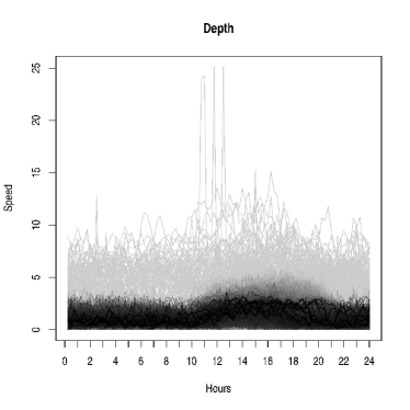
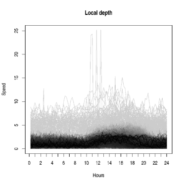
For this example we use a data set obtained from the Col De la Roa (Italy) meteorological station available at intra.tesaf.unipd.it/Sanvito. We concentrate on the wind speed recorded regularly every minutes in the years -. After removing incomplete days we obtain time series of length . We apply the modified half-region depth and the local modified half-region depth with , which corresponds to the quantile order of the empirical distribution of the sup norm between two time series.
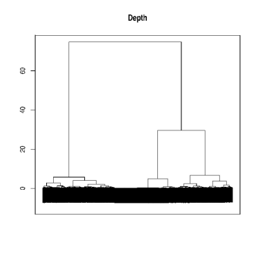
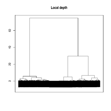
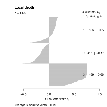
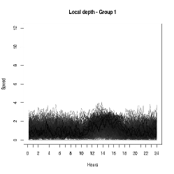
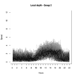
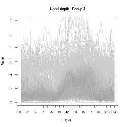
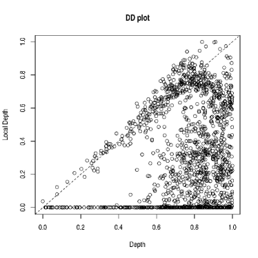
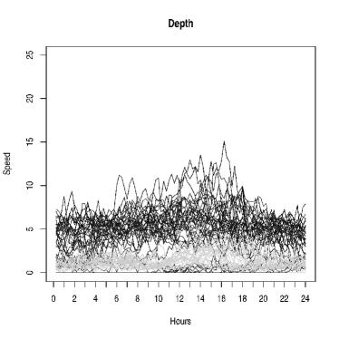
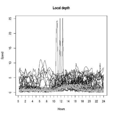
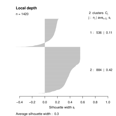
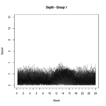
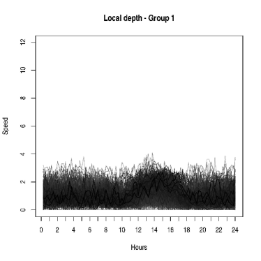
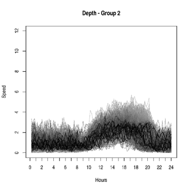
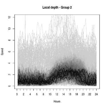
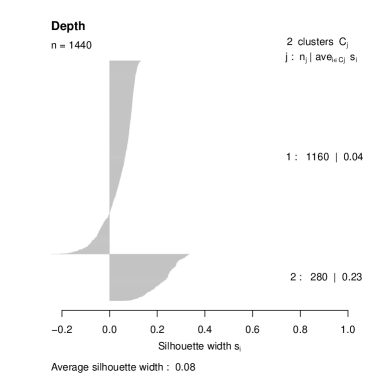
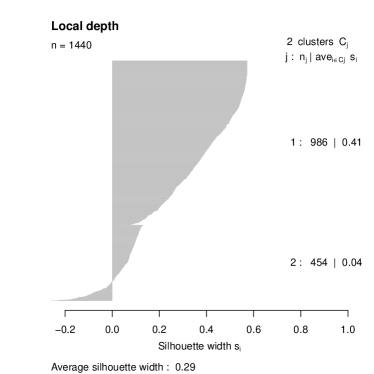
The two depths provide very different ranking for most series, while some ranks are preserved, see the Figure 4 in the Appendix where we report the DD plot. This is confirmed by the plots in Figure 1 where each series is plotted with a different color and width according to its rank, darker and wider means higher rank. We also investigate the possible presence of subgroups or structures. At this aim, we evaluate the dissimilarity measures based on the local modified half-region depth and modified half-region depth and run a hierarchical cluster analysis based on the Ward distance. In Figure 2 the dendrograms and the silhouette graphs are reported. Inspections of the dendrograms and several silhouette plots (not reported) shows that two groups are suggested by the modified half-region depth while three groups are supported by the local version. The classification is very different. Groups based on depth dissimilarity are very similar and they do not identify different pattern (see Figure 7 in the Appendix), while, the first group provided by local depth dissimilarity is characterized by days of wind calm with modest changes during the day; the second group shows an interesting pattern during the day: wind calm during the night and in the early morning with almost absence of wind between 8am-10am, moderate wind speed for the rest of the day until 9pm. The third group is formed by days with higher wind speed, with variability during the day and picks. Further comments and analysis are performed on this data set and reported in the Appendix.
5 Concluding remarks
Statistical data depth provides appropriate tools for the analysis of complex datasets such as functional data. However, since the nature of depth functions the analysis is not very suited for non homogeneous data, where subgroups/substructures are present. Instead, local depth is able to capture local features of the data and to provide a better analysis of the observations. Local modified half-region depth proved to be a suitable tool for the analysis of functional data as well as high dimensional data. Hierarchical clustering can be easily performed using similarity measures based on local modified half-region depth, classification is also straightforward but not reported in this work.
Acknowledgements
All statistical analysis were performed on SCSCF (www.dais.unive.it/scscf), a multiprocessor cluster system owned by Ca’ Foscari University of Venice running under GNU/Linux.

Appendix
Section A studies the properties of the local half-region depth in the finite dimensional case; Section B continues the example illustrated in Section 4 with further comments and figures. Section C shows an example based on individual household electric power consumption and Section D analyzes the out5d data set which contains data collected from remote sensing devices. In this last example a short illustration of the R package ldfun is provided. Finally, Section E contains all the proofs.
Appendix A Properties of the local half-region depth in the finite dimensional case
The half-region depth is invariant with respect to translations and some types of dilation. Let be a positive (or negative) definite diagonal matrix and , then
The local half-region depth exhibit the same type of invariance if the vector is transformed accordingly, i.e.,
On the other hand, if we restrict the values of always to be equal, than the local half-region depth is invariant to translations and only dilation , where is a constant scalar and is the identity matrix. This is, since we use one measure for all the slabs. In this particular situation, the same type of invariance as the half-region depth could be achieved by a componentwise standardization of the data. In practice, only asymptotic invariance can be obtained using a scale estimates for each of the component. The Median Absolute Deviation, without consistency constant could be used effectively.
In the rest of this subsection we study the main properties of the local half-region depth in the finite dimensional case. Most of the propositions are extensions of the results presented in López-Pintado and Romo [2011]. The proofs are reported in the Appendix. We start by describing the behaviour of the local half-region depth as function of the parameter.
Proposition 11
Let be the local half-region depth. Then, for any fixed
-
i.
if (), ;
-
ii.
for any vector such that , ;
-
iii.
;
-
iv.
.
Proofs are available in Section E. In the analysis of a data set, the vector could be chooses by considering the variability of each variable. For instance, () could be set as the quantile of the empirical distribution of the distance between all pairs of observations in the coordinate. In practice, quantile order in the interval - proved to be effective in most situations.
In the univariate case, the local half-region depth is equivalent to the local halfspace depth.
Proposition 12
For the local half-region depth can be expressed as
and it is equivalent to the local halfspace depth.
The local half-region depth decreases to zero when the point tends to infinity.
Proposition 13 (Vanishing at infinity)
Let and then
It is a continuous function when the underlying distribution is absolutely continuous.
Proposition 14
is an upper semicontinuous function. Moreover, if is absolutely continuous then is continuous.
Let be a sample of size from the random vector , and and be the corresponding empirical probability and distribution function respectively. In the next proposition we establish the consistency of the empirical local half-region depth and of its maximizer.
Proposition 15
is uniformly consistent:
Furthermore, if is uniquely maximized at and is a sequence of random variables with , then
Appendix B Wind speed
Hereafter, we report some more information regarding the example based on the wind speed data set. Figure 4 presents the DD-plot of the local depth versus the depth. When only one group is present in the data, almost all observations have the same ranks. In our case, most of the points are on the right bottom corner, which means they have high rank in the depth but low rank according to the local depth. Figure 5 shows the most unusual patterns and the most common patterns as identified by the modified half-region depth and the local modified half-region depth. The local version correctly identifies the serie with very high picks and other series with high variability, all belonging to the rd cluster, while the modified half-region depth identifies curves which belong to its nd cluster, see Figure 7 left panel. Silhouette plot based on two groups for local depth are reported in Figure 6. The two groups split seems the best clustering provided by depth, while, local depth suggests a three groups split as shown in the main document at Figure 2. Finally, for completeness, we show the clustering obtained by two groups split for both depth and local depth in Figure 7.
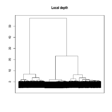
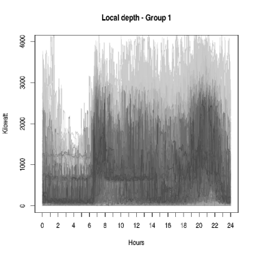
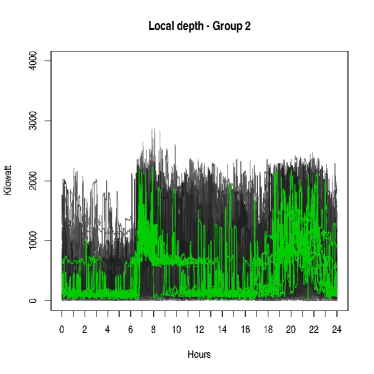
Appendix C Individual household electric power consumption
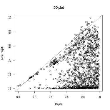
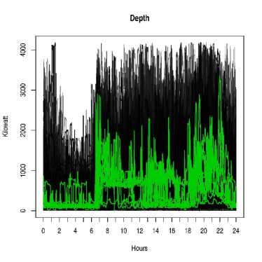
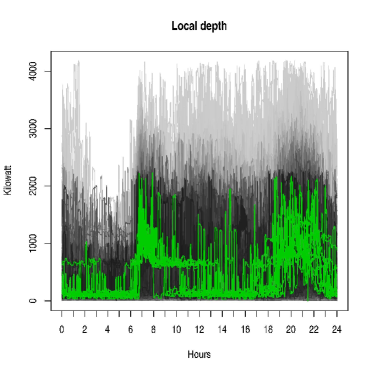
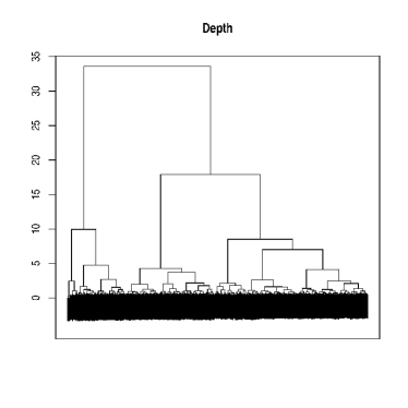
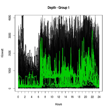
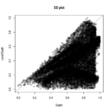
This archive contains measurements gathered between December and November ( months) on individual household electric power consumption [Bache and Lichman, 2013], an it is available at their website. Here we concentrate on global active power, i.e., household global minute-averaged active power in kilowatt. After removing 2 days which contain missing values and rearranging the data we obtain time series each based on observations. Figure 8 reports the DD-plot. Since the possible presence of two groups, the ranks provided by the two procedures are different. In particular, the local version provides more insight on the structures, high ranks are associated with a specific pattern, highlighted in green in figures, where consumption is almost null during the night, reaches a pick around 7am-8am, return to be null or with a moderate load in the early afternoon and return to have a higher consumption between 7pm and 11pm; see Figure 9. Figure 10 contrasts the dendogram and the silhouette plots provided by depth (left panels) and local depth (right panels) and Figure 11 shows the curves according to group membership. The differences are not very marked, however local depth provides a better job, in one group the trajectories with common consumptions, with a particular pattern as described above and picks of consumptions below 2Kw, in the other group the consumption tends to be high during all times.

Appendix D out5d
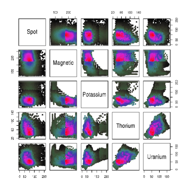
In this section we explore the out5d data set available at davis.wpi.edu/xmdv/datasets/out5d.html. It is a collection of 16384 observations along five dimensions collected from remote sensing devices in a particular region in Western Australia on a grid. The 5 variables are Spot, Magnetics and 3 bands of radiometrics which highlight Potassium, Thorium and Uranium. We concentrate on the local modified half-region depth method and we illustrate the use of the R package ldfun available upon request to the author. We first load the required packages
> require(ldfun)> require(cluster) and the data set from the original source
> url <- "http://davis.wpi.edu/~xmdv/datasets/out5d.tar.gz"> download.file(url, destfile="./out5d.tar.gz")> untar("out5d.tar.gz")> out5d <- read.table("./out5d.okc", header=FALSE, skip=7)> colnames(out5d)<-c("Spot", "Magnetic", "Potassium", "Thorium", "Uranium") The next function will be used to normalize the (local) depth in the interval
> normalize <- function(x) {+ x <- (x - min(x))/(max(x) - min(x))+ return(x)+ } The function quantile.localdepth.functional evaluates the distance between to curves using as default the sup norm, and return specific quantiles of its distribution. If size=TRUE, all the distances are also reported. The argument byrow=TRUE means that the observations are by rows and variables are on the columns, this is the default setting.
> tau <- quantile.localdepth.functional(out5d,+ probs=c(0.1, 0.2, 0.3, 0.4, 0.05), byrow=TRUE, size=TRUE) Since, we have several observations, we approximated the empirical distribution functions by plotting the percentile of the distribution, see Figure 12.
> plot(seq(0,1,0.01), quantile(tau$stats, probs=seq(0,1,0.01)),+ type="l", xlab="Size",+ ylab="Empirical Cumulative Distribution Funtion")

To explore the data set we set to be the quantile order of the distances distribution. The modified half-region detph and the local modified half-region depth are evaluated in the same call as
> mhr3 <- localdepth.modhalfregion(x=out5d,+ tau=tau$quantile[3], byrow=TRUE) the resulting object is of class localdepth and it is well integrated with the methods available in the CRAN package localdepth. Others depth measures are available in the package, see its documentation. DD-plot is easy to obtain as follows (Figure 13)
> plot(mhr3)> abline(0,1,lty=2)
and a parallel plot which highlight the higher rank curves by colors (Figure 14) is obtained by
> parallelplot(mhr3, lattice=TRUE) If the argument lattice is TRUE then the function parallelplot from the lattice package is used, otherwise the standard matplot function is called. To plot the ranks obtained by the depth, the argument type should be set accordingly.
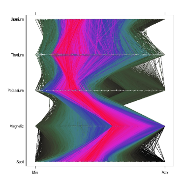
The plot point out the presence of a dense group of curves. As we will see later on, this group is characterize by low levels of Thorium and Uranium, and intermediate values of the others. A different representation is obtained by the function pairs after rearraging the observations according to their ranks and preparing a suitable palette colors, see Figure 15,
> omhr3 <- order(mhr3$localdepth)> oout5d <- out5d[omhr3,]> colmhr3 <- hsv(h = normalize(mhr3$localdepth),+ s = normalize(mhr3$localdepth),+ v = normalize(mhr3$localdepth), alpha = 1)> ocol <- colmhr3[omhr3]
> pairs(oout5d, col=ocol, pch=20)
We now turn our attention to the clustering problem. The function localdepth.similarity.modhalfregion provides the similarity measures based on both depth and local depth. The interface is very similar to the localdepth.modhalfregion.functional function, however we advise the user that this function run much slower and require a large amount of memory since it has to evaluate the (local) depth for points, hence for the sample sizes of the out5d data set we suggest its use in batch
> smhr3 <- localdepth.similarity.modhalfregion(x=out5d,+ tau=tau$quantile[3], byrow=TRUE) The function similarity2dissimilarity will convert a similarity matrix in a dissimilarity matrix using the tranformation suggested in Gower [1966], then the result is used as input for the hclust function
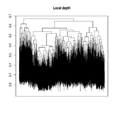
> dissimilarity <- similarity2dissimilarity(smhr3$localdepth)> mhrD <- hclust(as.dist(dissimilarity), method="ward") In the usual way we obtain the dendrogram (Figure 16 left panel)
> plot(mhrD, frame.plot=TRUE, labels=FALSE, ann=FALSE, main="Local depth")> title("Local depth") and the Silhouette plot (Figure 16 right panel)
> groups <- cutree(mhrD, k=3)> plot(silhouette(groups, dist=dissimilarity), main="Local depth")> ##plot(s3)
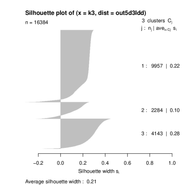
After inspection of the dendrogram and several silhouette plots we decide to stay with groups, to better characterize these groups we evaluate summary statistics on location and dispersion by
> sout5d <- split(out5d, groups)> lapply(sout5d, summary)> lapply(sout5d, function(x) apply(x, 2,+ function(y) diff(quantile(y, probs=c(0.25,0.75)))))> lapply(sout5d, function(x) apply(x, 2, function(y) sd(y))) some of these results are summarized in Tables 1 and 2.
| Group ID | Spot | Magnetic | Potassium | Thorium | Uranium |
|---|---|---|---|---|---|
| 1 | 100 (78) | 104 (74) | 90 (186) | 58 (29) | 55 (71) |
| 2 | 90 (47) | 208 (28) | 64 (23) | 55 (20) | 51 (17) |
| 3 | 62 (34) | 255 (0) | 60 (28) | 73 (25) | 82 (37) |
| Group ID | Spot | Magnetic | Potassium | Thorium | Uranium |
|---|---|---|---|---|---|
| 1 | 106 (53) | 122 (46) | 132 (85) | 61 (18) | 72 (39) |
| 2 | 89 (31) | 207 (17) | 62 (17) | 59 (17) | 56 (20) |
| 3 | 68 (26) | 253 (7) | 60 (19) | 75 (17) | 82 (23) |
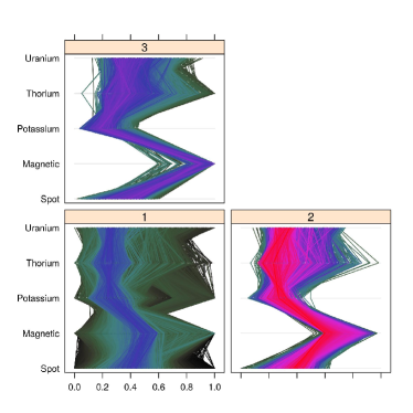
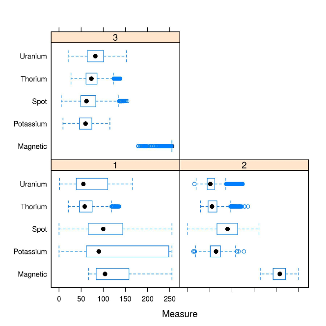
The first group is characterized by high levels of Spot and Potassium and low levels of Magnetic. The third group has extreme values of Magnetic, high levels of Thorium and Uranium, while low levels of Spot and Potassium. The second group presents somehow intermediate levels, with lower levels of Thorium and Uranium. Figure 17 reports the parallel plots of the groups where we can appreciate some of these characteristics
> myPanel <- function(x, col, ok, ...) {+ pp <- which.packet()+ panel.parallel(x, col=col[ok==pp], ...)+ }> ogroups <- groups[omhr3]> parallelplot(~oout5d | factor(ogroups), panel=myPanel,+ ok=ogroups, col=ocol, scales=list(x="same"))
To better highlight differences among the groups, we used the following code repeated for each variable
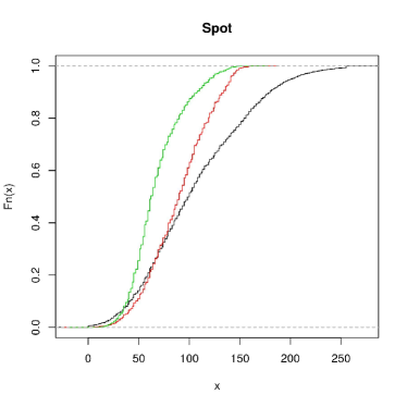
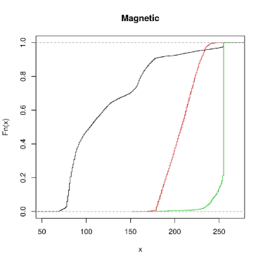
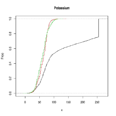
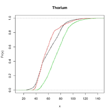
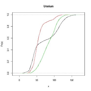
> plot(ecdf(sout5d[[1]]$Spot), pch="", verticals=TRUE, main="Spot")> lines(ecdf(sout5d[[2]]$Spot), pch="", col=2, verticals=TRUE)> lines(ecdf(sout5d[[3]]$Spot), pch="", col=3, verticals=TRUE) which produces Figure 18 on the Empirical cumulative distribution function of each variable conditional to group membership. These plots confirm our findings, the first group is characterized by high values of Spot and Potassium and low values of Magnetic, while the third group has very high levels of Magnetic, high levels of Thorium and low levels of Spot.
Finally, Figure 19 obtained with the following code
> out5dlattice <- data.frame(Measure=unlist(out5d),+ Cluster=rep(groups, times=ncol(out5d)),+ Variable=rep(c("Spot", "Magnetic", "Potassium", "Thorium", "Uranium"),+ each=nrow(out5d)))> bwplot(Variable~Measure | factor(Cluster), data=out5dlattice) presents box-plot of the variables conditional on group membership.
Appendix E Proofs
Proof of Proposition 11.
-
i.
The result follows since for all which implies . The same holds for the other component.
-
ii.
The first inequality holds since and for all vector while the second inequality holds since for all .
-
iii.
The result holds since by definition for .
-
iv.
we have
where is the line parallel to the axes and passing trough the point . Similarly for the other components of the half-region depth. Then and hence the result.
Proof of Proposition 12. The result follows immediately from the specialization of equations (1) to the case and the definition of the local half-region depth.
Proof of Proposition 13. The first result follows since Proposition 11 implies and Proposition 2 of López-Pintado and Romo [2011]. Similar motivation leads to the second statement.
Proof of Proposition 14. To prove that is upper semicontinuous we show that , when . Let and , and similarly and .
We will show that
which, together with the same result for the sequence of is sufficient to establish the continuity of . In fact,
Since , for the first term we have,
since and are disjoint sets.
Proof of Proposition 15. For the first statement we have that
is small than
| (2) |
and we will show that both terms will goes to zero, uniformly almost surely. In fact, using the Inclusion-Exclusion formula and rearranging the terms
Notice that the number of terms is finite and do not depend on sample size; applying Glivenko-Cantelli’s theorem in , each terms on the right hand side of the expression goes to zero, uniformly almost surely. Similar result holds for the second term of 2. This proves the first statement of the proposition.
We prove already that is an upper semicontinuous function that and if is uniquely maximized at , we have that for every , . To prove that , it is sufficient to establish that
which leads to the second statement of the proposition.
Proof of Proposition 5.
-
i.
By the definition of we have that and hence . Similar results holds for the epigraph which leads to the statement.
-
ii.
Let be the function always equals to and be the function always equals to . Then, by definition of and we have and . Furthermore, and together with the result at point i. lead to the inequalities.
-
iii.
We notice that, if then .
-
iv.
We notice that, if then .
Proof of Proposition 6. The first result holds since 5 implies and Proposition 5 of López-Pintado and Romo [2011]. Similar motivation leads to the second statement.
Proof of Proposition 7. To prove that is upper semicontinuous we show that , where .
To establish the continuity of the functional in with respect to the supremum norm it is sufficient to prove that both and are continuous. We prove the continuity of the first term, the prove is similar for the second term. We have to see that if then . Recall that,
Considering that the marginals of the distribution are continuous it is easy to prove that
| and | |||
Hence is a continuous function.
Proof of Theorem 8. The random variable corresponding to the local half-region depth can be expressed as
| by the law of large numbers and the continuity of the minimum, | |||
and then the result.
Proof of Theorem 9. Without loss of generality we assume that , is the empirical probability of random curves sampled from the stochastic process with probability , and given a measurable function we write for the mean process and for the expectation of with respect to , i.e., .
We define two families of measurable functions , and, similarly, where
We have,
where and for some positive constant . The second term converges almost surely to zero when tends to infinity by Proposition 6, hence we have to establish that the first term goes to zero almost surely for a given sufficiently large. At this aim we note that,
Hence, it is sufficient to prove that the two families and are P-Glivenko Cantelli Kosorok [2008, section 2.8.8]. Here we show the result for , similar prove can be obtain for . We prove that the bracketing number is finite, then Theorem 2.2 of Kosorok [2008] leads to the result. Given , we need to construct a finite number of functions that determine the -brackets , covering the family and such that . Hence, let fix an , then there exists such that by (i) we have
when . By the equicontinuity of , given , we let and there exists , such that if then for every . Consider the set of functions defined as constants in the intervals , , , , , and taking values in the sequence: , , , , , , , . The total number of possible functions that can be constructed like this is finite and we denote them as . Define the following set of indicator functions . This set of functions allows us to construct -brackets that cover the family . Since is finite this implies that the bracketing number is finite.
References
- Agostinelli and Romanazzi [2008] C. Agostinelli and M. Romanazzi. Local depth of multidimensional data. Working Paper 2008.3, Dipartimento di Statistica, Università Ca’ Foscari, Venezia, 2008.
- Agostinelli and Romanazzi [2011] C. Agostinelli and M. Romanazzi. Local depth. Journal of Statistical Planning and Inference, 141:817–830, 2011.
- Agostinelli and Rotondi [2015] C. Agostinelli and R. Rotondi. Analysis of macroseismic fields using statistical data depth functions: considerations leading to attenuation probabilistic modelling. Bulletin of Earthquake Engineering, pages 1–16, 2015. doi: 10.1007/s10518-015-9778-2.
- Bache and Lichman [2013] K. Bache and M. Lichman. UCI machine learning repository, 2013. URL http://archive.ics.uci.edu/ml.
- Chakraborty and Chaudhuri [2014] A. Chakraborty and P. Chaudhuri. On data depth in infinite dimensional spaces. Annals of the Institute of Statistical Mathematics, 66(2):303–324, 2014.
- Cuevas [2014] A. Cuevas. A partial overview of the theory of statistics with functional data. Journal of Statistical Planning and Inference, 147:1–23, 2014.
- Ferraty and Vieu [2006] F. Ferraty and P. Vieu. Nonparametric Functional Data Analysis. Springer, New York, 2006.
- González-Manteiga and Vieu [2007] W. González-Manteiga and P. Vieu. Statistics for functional data. Computational Statistics and Data Analysis, 51:4788–4792, 2007.
- Gower [1966] J.C. Gower. Some distance properties of latent root and vector methods used in multivariate analysis. Biometrika, 53:325–338, 1966.
- Horváth and Kokoszka [2012] L. Horváth and P. Kokoszka. Inference for Functional Data With Applications. Springer, New York, 2012.
- Inselberg [1985] A. Inselberg. The plane with parallel coordinates. The Visual Computer, 1(2):69–91, 1985.
- Kosorok [2008] M.R. Kosorok. Introduction to Empirical Processes and Semiparametric Inference. Springer, 2008.
- Liu [1990] R.Y. Liu. On a notion of data depth based on random simplices. The Annals of Statistics, 18(1):405–414, 1990.
- Liu et al. [2006] R.Y. Liu, R.J. Serfling, and D.L. Souvaine. Data depth: robust multivariate analysis, computational geometry, and applications. AMS Bookstore, 2006.
- López-Pintado and Romo [2009] S. López-Pintado and J. Romo. On the concept of depth for functional data. Journal of the American Statistical Association, 104(486):718–734, 2009.
- López-Pintado and Romo [2011] S. López-Pintado and J. Romo. A half-region depth for functional data. Computational Statistics & Data Analysis, 55(4):1679–1695, 2011.
- Mosler and Polyakova [2012] K. Mosler and Y. Polyakova. General notions of depth for functional data. arXiv preprint, 2012. arXiv:1208.1981.
- Moustafa and Wegman [2006] R. Moustafa, and E. Wegman. Multivariate continuous data – parallel coordinates. In Graphics of Large Datasets, Statistics and Computing, pages 143–155. Springer New York, 2006.
- Rafalin et al. [2005] E. Rafalin, K. Seyboth, and D.L. Souvaine. Proximity graph depth, depth contours, and a new multimodal median. Technical Report TR-2005-5R, Department of Computer Science, Tufts University, 2005.
- Ramsay and Silverman [2006] J.O. Ramsay and B.W. Silverman. Functional Data Analysis. Springer, 2006.
- Serfling [2002] R.J. Serfling. Generalized quantile processes based on multivariate depth functions, with applications in nonparametric multivariate analysis. Journal of Multivariate Analysis, 83(1):232–247, 2002.
- Sguera et al. [2014] C. Sguera, P. Galeano, and R. Lillo. Spatial depth-based classification for functional data. TEST, 23(4):725–750, 2014.
- Tukey [1975] J.W. Tukey. Mathematics and picturing of data. In Proceedings of International Congress of Mathematics, volume 2, pages 523–531, 1975.
- Zuo and Serfling [2000] Y. Zuo and R.J. Serfling. General notions of statistical depth function. Annals of Statistics, 28(2):461–482, 2000.