Modeling the power consumption of a Wifibot and studying the role of communication cost in operation time
Abstract
Mobile robots are becoming part of our every day living at home, work or entertainment. Due to their limited power capabilities, the development of new energy consumption models can lead to energy conservation and energy efficient designs. In this paper, we carry out a number of experiments and we focus on the motors power consumption of a specific robot called Wifibot. Based on the experimentation results, we build models for different speed and acceleration levels. We compare the motors power consumption to other robot running modes. We, also, create a simple robot network scenario and we investigate whether forwarding data through a closer node could lead to longer operation times. We assess the effect energy capacity, traveling distance and data rate on the operation time.
1 Introduction
Nowadays, mobile robots are used in a variety of applications beginning from the most common ones like vacuum-cleaners, pool-cleaners and drones and extending to more complex like secure and rescue, and planet exploration [24]. The environmental monitoring is another application, where robots can be used to detect gas [16], air pollution [7], and mines [23]. The rescue mobile robot Quince has been developed to resolve technical issues in case of a nuclear plant accident [20]. NASA’s Mars Exploration Rovers is another robot which was used to discover Mars’ surface and water activity. In all these applications, the robots are powered by batteries and energy conservation is critical for the longevity of the project.
In order to design power-efficient methods for mobile robots, it is important to have a practical knowledge of the energy efficiency of the devices used. This paper provides some models of the global power consumption based on the utilization of major robot power consumers, such as the motors, the network adapter, the embedded controllers etc.. We carry out a set of experiments using a mobile robotic platform called Wifibot [2]. It is a modern commercial mobile robot which has been used in many research activities [5, 10, 22, 11, 21, 26]. We believe that the results would be helpful for people who work with other types of robots, as well as for researchers who work on the design of power efficient paths and scheduling techniques.
Our study has three major contributions.
We model the power consumption of several motors running modes using real experiments and we examine the role of acceleration in power cost. As far as we know, this is the first work which models the extra cost of acceleration in total power expense. The results show that this cost can grow the total power consumption up to 66% for the specific robot.
Second, we measure the power consumption utilizing other power consumers like the embedded system, the processor, the wireless network interface, and the camera. The results show that only the 25% of the total power is used for the motion, while the half is spent by the embedded system.
Third, we examine whether moving a robot to a new location and lowering the communication cost could conserve energy and in long-term could lead to longer operation times. We assume a simple scenario where a robot is used as relay which comes in between a robot with monitoring capabilities and a base station. The two robots adapt their communication ranges to shorter radius and, thus, consume less energy. The results show minor improvements compared to the case where a direct long communication range is used. Since these results are based on the specific robot, we present a number of generic conditions under which the reduced communication cost could result in longer operation time.
2 Related work
Energy efficiency is an important issue in mobile robotics and providing accurate power consumption models helps to the design of better algorithms to reduce the overall consumption. In this section, we summarize the most recent works related to energy efficiency in mobile robots.
A significant amount of works has been done in the area of energy efficient trajectories design. However, in these works, the motion consumption is considered as the unique power consumer in the design of the algorithms. In this paper, we show that the embedded system, as well as the processing and the communication consume significant amounts of energy. The authors in [17] focus on finding energy-efficient motion plans by determining velocities for predefined routes. In [25], optimal paths are computed with respect to the energy consumption of the robot. An efficient approximation algorithm that computes a path whose cost is within a user-defined relative error ratio is presented. Similarly to this work, energy-efficient motion planning problems are considered in [13, 14] and [15]. In these works, A* algorithm is used to construct optimized trajectory plans which are computed by dividing the path in segments; efficient angles and velocities are calculated for each segment. Regarding the same works, theoretical and experimental power consumption values are taken into account in [13] and [15, 14] respectively. However, only motion power is taken into account. Finally, an improved A* algorithm is presented in [31] which significantly reduces the energy expense in the authors examined scenario compared to the classic A* approach.
Energy savings can be also achieved by properly scheduling the robot operations. For example, in [4], an optimization method which controls both processor’s frequency and motor’s speed is introduced to avoid collisions. In other works, the energy consumption for each operation is modeled and parameterized as function of the operation execution time, and an energy-optimal schedule is derived by solving a mixed-integer nonlinear programming problem [29]. Since robots consist of several embedded systems that we also meet in a common computer, dynamically reconfiguring these systems to provide the required services with the minimum number of active devices, could lead to energy conservation [18]. These dynamic power management techniques are summarized in [3, 30] and they are out of the scope of this paper.
Morales et al. [19] model the power consumption of a skid-steer tracked mobile robot. The authors focus on modeling the power losses of dynamic friction since in this kind of robots the contact area with the ground is high. Energy scavenging technologies for mobile robots are discussed in [27]. The authors assess the feasibility of using these technologies by conducting experiments with a set of robotic vacuum cleaners. Vaussard et al. [28] study new technologies that could lead to energy reduction of domestic mobile robots. They validate their study by analyzing the power consumption of seven vacuum-cleaning robots. In [18] The authors present a case study of a mobile robot energy consumption, named Pioneer 3DX, and they introduce some energy conservation techniques. The consumption of other robot components is taken into account in the experimental measurements. However, motor acceleration is not considered. As it is claimed in this paper as well as in other works, the communication cost can be saved by placing intermediate robots (nodes) between the robot which transfers data and a base station. It is assumed that transmitting a high volume of data could save the motion cost to move closer to the transfer robot. However, this assumption is not verified or quantified.
3 Mobile robot architecture – Wifibots
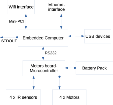
A common mobile robot consists of some essential components, like the microcontroller, the motors, the embedded computer, one or more sensors, and the batteries. In some robots the embedded computer and the microcontroller refer to the same device. Several other peripherals are connected to the microcontroller or to the embedded computer such as communication interfaces, and output devices. The microcontroller is a special purpose computer and its main responsibility is to directly communicate with the motors and adjust their power levels. Usually, the microcontroller provides a programming interface to the embedded computer through which a user commands the main robot functionalities. Other minor functionalities are already embedded in the firmware of the microcontroller as for example the monitoring of the motors temperature. The embedded computer is a general purpose machine with much higher computational capabilities. Peripheral devices like network adapters, monitors, keyboards, cameras etc. are connected to this machine. The whole system is usually powered by batteries which are located in the robot chassis. Some robots also use solar surfaces to partially recharge the batteries and delay their exhaustion [12]. Depending on the batteries storage capacity and the consumption of the components, a robot may operate from a few minutes to several hours.
Figure 1 illustrates an overview of the Wifibot architecture. The embedded computer plays the role of a motherboard in common computers where all peripherals are connected on it. A low consumption x86 processing unit and a flash disk are used to reduce power consumption. The embedded computer communicates with a motor board through a serial port. The motor board plays the role of the microcontroller and the power regulator. It is responsible of handling low-level controls of the motors and the IR distance sensors. The power supply is connected to the motor board through which is distributed to the microcontroller and the other robot components [1].
4 Experimental Setup & Results
4.1 Setup
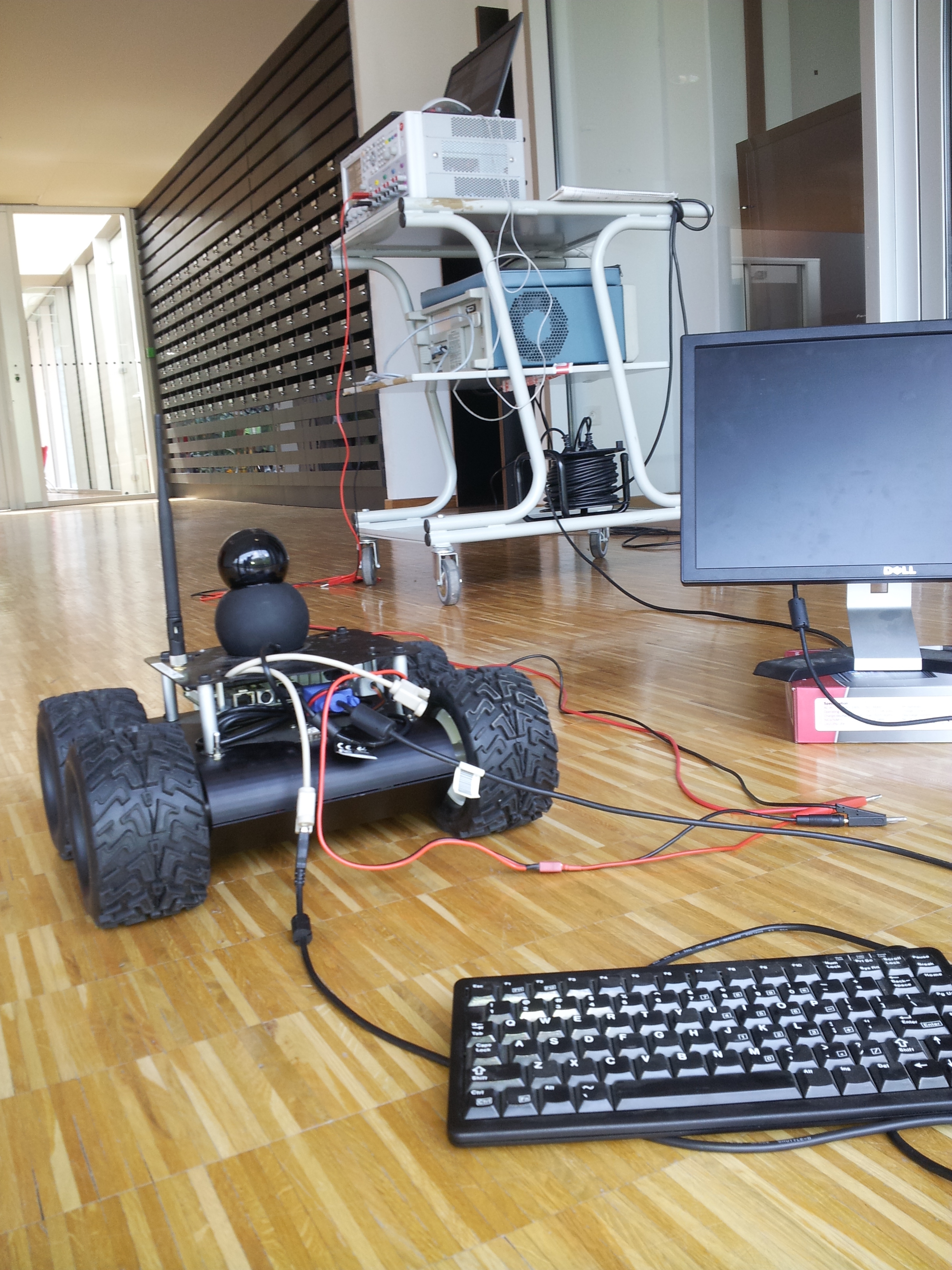
All the experiments were carried out using a Wifibot mobile robot, a power analyzer connected to the robot, a keyboard, and a monitor. The third version of a stock Wifibot was used which weighs approximately 4kg including lithium iron phosphate batteries. The robot’s maximum speed is 0.9 m/s. For the needs of our experiments we bypassed the battery assembly by directly powering up the robot with the power analyzer. A cable was used to connect the robot with the power analyzer as it is illustrated in Figure 2. The cable was long enough in order to move the robot many meters away without disconnecting the analyzer. The analyzer was placed on a cart pushed by a person in case we wanted to travel very long distances. The commands were given by a USB keyboard and the standard output was displayed on an external VGA monitor. Both the keyboard and the monitor were detached before the robot starts moving. A number of scripts was developed to control the robot’s maximum traveling distance and speed. After each experiment we used to reposition the robot to its initial position, reconnecting the keyboard and the monitor. We exploited the output log files of the power analyzer to calculate the power at each instance of the experiment. Particularly, one value was taken every 0.1024msec for some seconds. All the experiments took place on a flat surface of a clean non-slippery parquet-style floor providing a good grip without spinning while accelerating or moving.
4.2 Assessing motion power consumption
In this section, we measure the overall power consumption based on the utilization of the motors. We compare the results to different robot running modes. We separate the power analysis in two parts. In the first part, we analyze the power increase caused by acceleration, while in the second part we model the normal (constant) consumption at a given speed.
The power consumed by a mobile robot is the sum of the power consumed by the motors (mechanical power) and the power consumed by the embedded devices (see Formula 1). The mechanical power (i.e, ) is used to accelerate and maintain a constant speed. It is expected to be a linear function which depends on the robot mass , the speed , a ground friction constant , and the acceleration of gravity [18, 14].
| (1) |
reports to the power loss due to transformation from electrical to mechanical energy and is the power consumption of the embedded devices. Assuming that is negligible compared to the other power consumers, the total power expense is a linear function of the speed. The robot’s mass can, also, affect the energy cost during the acceleration.
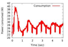
Figure 3 illustrates the power consumption of the robot for 5 seconds and different speed levels. Initially it starts from a stationary position, it accelerates reaching a maximum given speed, and it keeps moving on a straight line for some seconds. The displayed consumption also includes the power consumption of the integrated system which is about 23 Watts (idle mode). All the other unnecessary components (camera, network adapters etc.) are switched off during all the experiments. Each experiment was carried out several times (runs) and the average results are presented. The results show that the power while accelerating may be more than two times higher than normal consumption.
As we mentioned before, we split the recorded power instances in two parts. The first part concerns the acceleration power while the second one concerns the power needed to maintain a constant speed. By analyzing the monitoring data and applying the least square method we conclude that the power used for acceleration is given by:
| (2) |
where is the given maximum speed. This is the average power during the acceleration phase.
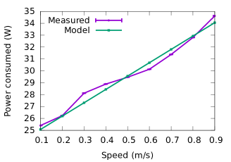
When the given speed is reached, the power consumption presents a sinusoidal periodicity which is more clear at lower speeds. Each run of an experiment consists of some thousands of values stored in the power analyzer. Excluding acceleration and computing the average value for each instance of speed, we get that the power consumption for a given speed is given by:
| (3) |
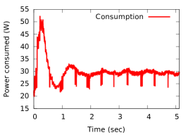
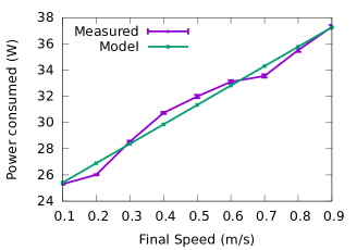
Figure 4 depicts the power consumption during and after acceleration. The average experimental values as well as the fitting line are presented. The average power during acceleration may be up to 9.5% higher than traveling at constant speed. This increase in power consumption is high at high speeds and low at low speeds. Combining Formulas (2) and (3), the total energy cost of a single run is given by:
| (4) |
where and is the total moving time and the acceleration time respectively. Since after acceleration, the robot performs a linear motion, Formula (4) can be also written as:
| (5) |
where and is the total traveling distance and the distance traveled during acceleration respectively. From Formulas (4) and (5) we can conclude that the extra energy cost due to acceleration is not negligible unless low-speed or very long runs are performed.
To clarify this statement we conduct another experiment where we vary the speed and the traveling step (distance traveled before the robot stops). The results are presented in Figure 5. We can observe that the energy is higher for lower speeds since the time to travel the distance is longer. When the distance is 10 meters, we distinguish an extra case to assess the effect of acceleration in total consumption. In this case, the robot travels the distance with equal steps of 1 meter each. The robot stops at the end of each step. The results show that the energy consumption in high speeds is up to 66% higher than completing the task in one step.

4.3 Activating other components
Table 1 summarizes the global power while utilizing a number of robot components and compares the results to the consumption when the robots moves at maximum speed. In particular, in addition to the motion power consumption, we measure the power consumption when (a) the robot is idle, (b) it is transmitting data using the highest possible bandwidth of the wifi interface (802.11g), (c) a video is taken using the integrated webcam (jpeg format), and (d) a CPU core is stressed with maximum load. The power values in parenthesis are the net values without including the idle power consumption.
The results reveal that more than 50% of the overall power is consumed when the robot stays idle. This is actually the power consumption of the embedded system and equals to the minimum possible consumption of the robot while it is in power on mode 111some energy savings may be achieved if some of the computer components, like cpu cores, usb, infrared etc, are turned off. The embedded system power consumption is apparently high, but is similar to that of other mobile robots, like the one tested in [18]. The motion consumption comes second with 25% of the overall power while the network consumption, the webcam usage and the CPU stress test are in third, fourth and fifth place respectively.
| Function | Power (W) | Max. Motion (%) | Overall (%) |
|---|---|---|---|
| Max. Motion | 33.98 (10.68) | 0 | 24.85 |
| Idle | 23.3 | 118.16 | 54.21 |
| Network | 27.7 (4.4) | -58.8 | 10.24 |
| Video | 25.8 (2.5) | -76.59 | 5.82 |
| CPU | 25.4 (2.1) | -80.34 | 4.89 |
5 The communication effect on the operation time
In our measurements wifi transmission consumes about 10% of the total power consumption. Other experimental measurements of wifi interfaces have shown that power consumption while transmitting or receiving costs only some nanowatts per bit [6, 8]. However, usually network devices adapt their transmission power to the trasmission range in order to conserve some energy. We take advantage of this capability and we study whether a reduced distance between the transmitter and the receiver could lead, in long-term, to lower total power consumption and, thus, to longer operation times.
We consider a simple scenario where a stationary robot, which is used for monitoring and communicates with a base station, decreases its transmission power forwarding its monitoring data through a nearby relay robot. Figure 6 illustrates the examined scenario. We assume that the stationary robot, annotated with “A”, is located far from the base station consuming a lot of energy for transmissions. Robot B is located close to A. The two robots are in the communication range of each other. We move robot B towards a midpoint between A and the base station, operating as relay node, an action which we would wish to decrease the consumption of monitoring robot and, thus, would increase the monitoring time.
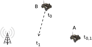
We assume that B’s movement starts at and stops at . During B’s movement, “A” communicates directly with the base station and for this period of time the total amount of energy it consumes is equal to the following sum:
| (6) |
where is the power consumption due to data transmission, is the sensing power consumption, and is the power consumption of the embedded system. is the amount of data transmitted per time unit. When “B” reaches its destination, it starts operating as relay node. From this moment its energy consumption is computed as follows:
| (7) |
where is the power consumption due to data reception.
is a non-fixed value which depends on transmitter’s power. The higher the power, the longer the transmission distance. , , and are fixed.
Assuming an even energy reduction of the initial battery storage, the lifetime of the network is computed by dividing the initial energy of the robot at by its energy consumption per time unit. The energy consumption per time unit is actually the average power consumption and it is annotated with .
The network lifetime depends on the initial energy of the two robots at and their power consumptions. According to the value of these parameters any of the two robots may die first interrupting the network activity. If robot A dies first then the network lifetime is given by:
| (8) |
where is the moving time of B and is the energy consumed by A while B is moving. is computed by choosing a transmission power capable of transmitting data to the base station with a very low bit error rate [9].
If robot B dies first, the network lifetime is computed by the following sum:
| (9) |
The first term is the moving time of B, the second term is the lifetime of B, and the third term is the time “A” can directly communicate with the base station after B’s death. If we assume that “B” dies at moment , then is the energy reduction of robot A during the period between and . is computed by Formula (10).
| (10) |
We compute the lifetime improvement over the initial scenario where B is not used as relay node at all. In this case the network lifetime would be equal to . We consider an initial battery capacity as it is specified in Wifibot V3 specifications [2], constant data bitrates from 10 to 100Mbit/sec, and a IEEE 802.11n power consumption model for and as it is experimentally measured in [8]. and are measured in nW/bit and they depend on the actual data bitrate (i.e., ). The higher the data rate, the lower the value of and . We summarize the parameters used in Table 2.
| Parameter | Values |
|---|---|
| (when not variable) | 480 kJ |
| (when variable) | 50 to 450 kJ |
| (when not variable) | 100Mbit/sec |
| (when variable) | 10, 54, 100Mbit/sec |
| (high trans. power) | 95, 24, 12nW/bit |
| (low trans. power) | 9.5, 2.4, 1.2nW/bit |
| 70, 18, 10nW/bit | |
| 100nW/bit | |
| travel. dist. (when variable) | 2 to 10m |
| travel. dist. (when not variable) | 10m |
| by Formula (5) | |
| speed | 0.9 m/sec |
We vary the initial energy capacity, the traveling distance and the data bitrate of either robot A or B for Formulas (8) and (9) respectively. According to these formulas, A or B may die first. For this reason, we distinguish two cases; in the first one, we keep constant the initial energy capacity of B, varying the initial capacity of A, while in the second one we do the opposite. The X axis of Figure 7a represents the initial energy of either A or B, when it is not constant.
The results are presented in Figure 7 and show minor lifetime improvements ranging from 0.5 to 4.5%. One could say that the operation time cannot improve a lot since the specific embedded system consumes a lot of power. However, our simulations revealed a higher, but still low improvement (up to 7.6%), considering an embedded system with the half of the power consumption of our specific robot. We omit these results since their trend is the same as in Figure 7; they only differ in terms of absolute values. The results, also, show that the lifetime presents a linear increase as the initial energy of robot B is growing. It means that considering higher energy capacities, the lifetime could be further improved.


6 Conclusion
In this paper, we modeled the power consumption of several running modes of a mobile robot called Wifibot. We conducted a number of experiments giving attention to specific motor running modes, such as acceleration and constant speeds. Based on the consumption of these running modes, we built models for acceleration and constant speeds. The results showed that if the robot stops frequently, the energy cost increases up to 66% mainly due to accelerations. Moreover, high energy efficiency is achieved at higher speeds. Even if these results are based on the specific robot, we believe that acceleration is, generally, an operation with high energy cost and, thus, its frequent use shortens the operation time. How much it affects performance depends on motors characteristics as well as on robot payload.
We extended our approach to a simulated experiment involving two robots that perform communication with a distant station. We examine whether a shorter communication link, and thus lower power consumption, could lead to longer operation times. We considered a simple scenario where a robot is moved between a distant node which is used for monitoring and a base station. The two robots adjust their communication ranges to shorter radius to conserve energy. The simulation results show that low operation time savings can be achieved for the specific robot. However, equations show that this technique could lead to better results if other robots with lower consumption of the embedded system or/and high energy storage units were used.
Acknowledgements
The authors gratefully acknowledge the comments received from Roman Igual during the experimentation setup and the help he provided using the IRCICA telecommunication platform (http://www.ircica.univ-lille1.fr).
References
- [1] Wifibot v3 datasheet. http://www.wifibot.com/download/2012/Wifibot_datasheetEN2012_V3.pdf.
- [2] Wifibots, mobile robots. http://www.wifibot.com/.
- [3] L. Benini, A. Bogliolo, and G. De Micheli. A survey of design techniques for system-level dynamic power management. Very Large Scale Integration (VLSI) Systems, IEEE Transactions on, 8(3):299–316, June 2000.
- [4] J. Brateman, Changjiu Xian, and Yung-Hsiang Lu. Energy-effcient scheduling for autonomous mobile robots. In Very Large Scale Integration, 2006 IFIP International Conference on, pages 361–366, Oct 2006.
- [5] M. Erdelj, T. Razafindralambo, and D. Simplot-Ryl. Covering points of interest with mobile sensors. Parallel and Distributed Systems, IEEE Transactions on, 24(1):32–43, Jan 2013.
- [6] L.M. Feeney and M. Nilsson. Investigating the energy consumption of a wireless network interface in an ad hoc networking environment. In INFOCOM 2001. Twentieth Annual Joint Conference of the IEEE Computer and Communications Societies. Proceedings. IEEE, volume 3, pages 1548–1557 vol.3, 2001.
- [7] Gabriele Ferri, Alessio Mondini, Alessandro Manzi, Barbara Mazzolai, Cecilia Laschi, Virgilio Mattoli, Matteo Reggente, Todor Stoyanov, Achim Lilienthal, Marco Lettere, et al. Dustcart, a mobile robot for urban environments: Experiments of pollution monitoring and mapping during autonomous navigation in urban scenarios. Proceedings of the IEEE International Conference on Robotics and Automation (ICRA 2010) Workshop on Networked and Mobile Robot Olfaction in Natural, Dynamic Environments, 2010.
- [8] Daniel Halperin, Ben Greenstein, Anmol Sheth, and David Wetherall. Demystifying 802.11n power consumption. In Proceedings of the 2010 International Conference on Power Aware Computing and Systems, HotPower’10, pages 1–, Berkeley, CA, USA, 2010. USENIX Association.
- [9] Jangeun Jun, P. Peddabachagari, and M. Sichitiu. Theoretical maximum throughput of ieee 802.11 and its applications. In Network Computing and Applications, 2003. NCA 2003. Second IEEE International Symposium on, pages 249–256, April 2003.
- [10] Christos Katsikiotis, Dimitrios Zorbas, and Periklis Chatzimisios. Connectivity restoration and amelioration in wireless ad-hoc networks: A practical solution. In Natalie Mitton, Antoine Gallais, Melike Erol Kantarci, and Symeon Papavassiliou, editors, Ad Hoc Networks, volume 140 of Lecture Notes of the Institute for Computer Sciences, Social Informatics and Telecommunications Engineering, pages 255–264. Springer International Publishing, 2014.
- [11] Ayumi Kawakami, Koji Tsukada, Keisuke Kambara, and Itiro Siio. Potpet: Pet-like flowerpot robot. In Proceedings of the Fifth International Conference on Tangible, Embedded, and Embodied Interaction, TEI ’11, pages 263–264, New York, NY, USA, 2011. ACM.
- [12] J.H. Lever, A. Streeter, and L.R. Ray. Performance of a solar-powered robot for polar instrument networks. In Robotics and Automation, 2006. ICRA 2006. Proceedings 2006 IEEE International Conference on, pages 4252–4257, May 2006.
- [13] Shuang Liu and Dong Sun. Optimal motion planning of a mobile robot with minimum energy consumption. In Advanced Intelligent Mechatronics (AIM), 2011 IEEE/ASME International Conference on, pages 43–48, July 2011.
- [14] Shuang Liu and Dong Sun. Modeling and experimental study for minimization of energy consumption of a mobile robot. In Advanced Intelligent Mechatronics (AIM), 2012 IEEE/ASME International Conference on, pages 708–713, July 2012.
- [15] Shuang Liu and Dong Sun. Minimizing energy consumption of wheeled mobile robots via optimal motion planning. Mechatronics, IEEE/ASME Transactions on, 19(2):401–411, April 2014.
- [16] D. Martinez, J. Moreno, M. Tresanchez, M. Teixido, J. Palacin, and S. Marco. Preliminary results on measuring gas and wind intensity with a mobile robot in an indoor area. In Emerging Technology and Factory Automation (ETFA), 2014 IEEE, pages 1–5, Sept 2014.
- [17] Yongguo Mei, Yung-Hsiang Lu, Y.C. Hu, and C.S.G. Lee. Energy-efficient motion planning for mobile robots. In Robotics and Automation, 2004. Proceedings. ICRA ’04. 2004 IEEE International Conference on, volume 5, pages 4344–4349 Vol.5, April 2004.
- [18] Yongguo Mei, Yung-Hsiang Lu, Y.C. Hu, and C.S.G. Lee. A case study of mobile robot’s energy consumption and conservation techniques. In Advanced Robotics, 2005. ICAR ’05. Proceedings., 12th International Conference on, pages 492–497, July 2005.
- [19] J. Morales, J. L. MartÃnez, A. Mandow, A. J. GarcÃa-Cerezo, and S. Pedraza. Power consumption modeling of skid-steer tracked mobile robots on rigid terrain. IEEE Transactions on Robotics, 25(5):1098 –1108, 2009.
- [20] Keiji Nagatani, Kiribayashi S., Okada Y., Tadokoro S., Nishimura T., Yoshida T., Koyanagi E., and Hada Y. Redesign of rescue mobile robot quince. In Safety, Security, and Rescue Robotics (SSRR), 2011 IEEE International Symposium on, pages 13–18, Nov 2011.
- [21] Roberto Quilez, Adriaan Zeeman, Nathalie Mitton, and Julien Vandaele. Docking autonomous robots in passive docks with Infrared sensors and QR codes. In International Conference on Testbeds and Research Infrastructures for the Development of Networks & Communities (TridentCOM), Vancouver, Canada, June 2015.
- [22] Tahiry Razafindralambo, Thomas Begin, Marcelo Dias de Amorim, IsabelleGuérin Lassous, Nathalie Mitton, and David Simplot-Ryl. Promoting quality of service in substitution networks with controlled mobility. In Hannes Frey, Xu Li, and Stefan Ruehrup, editors, Ad-hoc, Mobile, and Wireless Networks, volume 6811 of Lecture Notes in Computer Science, pages 248–261. Springer Berlin Heidelberg, 2011.
- [23] K. Schreiner. Landmine detection research pushes forward, despite challenges. Intelligent Systems, IEEE, 17(2):4–7, Mar 2002.
- [24] R. Siegwart, I.R. Nourbakhsh, and D. Scaramuzza. Introduction to Autonomous Mobile Robots. Intelligent robotics and autonomous agents. MIT Press, 2011.
- [25] Zheng Sun and J.H. Reif. On finding energy-minimizing paths on terrains. Robotics, IEEE Transactions on, 21(1):102–114, Feb 2005.
- [26] Anne-Sophie Tonneau, Nathalie Mitton, and Julien Vandaele. How to choose an experimentation platform for wireless sensor networks? . Elsevier Adhoc networks, 30:12, July 2015.
- [27] Florian Vaussard, Michael Bonani, Philippe Rétornaz, Alcherio Martinoli, and Francesco Mondada. Towards autonomous energy-wise robjects. In Roderich Groß, Lyuba Alboul, Chris Melhuish, Mark Witkowski, TonyJ. Prescott, and Jacques Penders, editors, Towards Autonomous Robotic Systems, volume 6856 of Lecture Notes in Computer Science, pages 311–322. Springer Berlin Heidelberg, 2011.
- [28] Florian Vaussard, Philippe Rétornaz, David Hamel, and Francesco Mondada. Cutting down the energy consumed by domestic robots: Insights from robotic vacuum cleaners. In Guido Herrmann, Matthew Studley, Martin Pearson, Andrew Conn, Chris Melhuish, Mark Witkowski, Jong-Hwan Kim, and Prahlad Vadakkepat, editors, Advances in Autonomous Robotics, volume 7429 of Lecture Notes in Computer Science, pages 128–139. Springer Berlin Heidelberg, 2012.
- [29] A. Vergnano, C. Thorstensson, B. Lennartson, P. Falkman, M. Pellicciari, Chengyin Yuan, S. Biller, and F. Leali. Embedding detailed robot energy optimization into high-level scheduling. In Automation Science and Engineering (CASE), 2010 IEEE Conference on, pages 386–392, Aug 2010.
- [30] Li-Chuan Weng, XiaoJun Wang, and Bin Liu. A survey of dynamic power optimization techniques. In System-on-Chip for Real-Time Applications, 2003. Proceedings. The 3rd IEEE International Workshop on, pages 48–52, June 2003.
- [31] Zhao Xu, Su Zhong, and Dou Lihua. A path planning method with minimum energy consumption for multi-joint mobile robot. In Control Conference (CCC), 2014 33rd Chinese, pages 8326–8330, July 2014.