Clustering time series under the Fréchet distance

Abstract

The Fréchet distance is a popular distance measure for curves. We study the problem of clustering time series under the Fréchet distance. In particular, we give $(1+{\varepsilon})$-approximation algorithms for variations of the following problem with parameters $k$ and $\ell$. Given $n$ univariate time series $P$, each of complexity at most $m$, we find $k$ time series, not necessarily from $P$, which we call cluster centers and which each have complexity at most $\ell$, such that (a) the maximum distance of an element of $P$ to its nearest cluster center or (b) the sum of these distances is minimized. Our algorithms have running time near-linear in the input size for constant ${\varepsilon},k$ and $\ell$. To the best of our knowledge, our algorithms are the first clustering algorithms for the Fréchet distance which achieve an approximation factor of $(1+{\varepsilon})$ or better.

Keywords: time series, longitudinal data, functional data, clustering, Fréchet distance, dynamic time warping, approximation algorithms.

1 Introduction

Time series are sequences of discrete measurements of a continuous signal. Examples of data that are often represented as time series include stock market values, electrocardiograms (ECGs), temperature, the earth’s population, and the hourly requests of a webpage. In many applications, we would like to automatically analyze time series data from different sources: for example in industry 4.0 applications, where the performance of a machine is monitored by a set of sensors. An important tool to analyze (time series) data is clustering. The goal of clustering is to partition the input into groups of similar time series. Its purpose is to discover hidden structure in the input data and/or summarize the data by taking a representative of each cluster. Clustering is fundamental for performing tasks as diverse as data aggregation, similarity retrieval, anomaly detection, and monitoring of time series data. Clustering of time series is an active research topic [4, 12, 22, 42, 47, 55, 57, 60, 63, 66, 67, 68, 71, 72, 73] however, most solutions lack a rigorous algorithmic analysis. Therefore, in this paper we study the problem of clustering time series from a theoretical point of view.

Formally, a time series is a recording of a signal that changes over time. It consists of a series of paired values $(w_{i},t_{i})$, where $w_{i}$ is the $i$th measurement of the signal, and $t_{i}$ is the time at which the $i$th measurement was taken. A common approach is to treat time series data as point data in high-dimensional space. That is, a time series $S_{j}=(w_{1},t_{1}),\dots,(w_{m},t_{m})$ of the input set is treated as the point $S^{*}_{j}=(w_{1},\dots,w_{m})$ in $m$-dimensional Euclidean space. Using this simple interpretation of the data, any clustering algorithm for points can be applied. Despite it being common practice (for a survey, see [57]), it has many limitations. One major drawback is the requirement that all time series must have the same length and the sampling must be regular and synchronized. In particular, the latter requirement is often hard to achieve.

In this paper, we follow a different approach that has also received much attention in the literature. In order to formulate the objective function of our clustering problem, we consider a distance measure that allows for irregular sampling and local shift and that only depends on the “shape” of the analyzed time series: the Fréchet distance. The Fréchet distance is defined for continuous functions $f:[0,1]\rightarrow{\rm I\!R}$. Two functions $f,g$ have Fréchet distance at most $\delta$, if one can move simultaneously but at different and possibly changing positive speed on the domains of $f$ and $g$ from $0$ to $1$ such that at all times $|f(x)-g(y)|\leq\delta$, where $x$ and $y$ are the current positions on the respective domains. The Fréchet distance is the infimum over the values $\delta$ that allow such a movement. For a formal definition, see Section 2.1. The Fréchet distance between two monotone functions $f,g:[0,1]\rightarrow{\rm I\!R}$ equals the maximum of $|f(0)-g(0)|$ and $|f(1)-g(1)|$. This also implies, that the Fréchet distance between two functions is completely determined by the sequence of local extrema ordered from $0$ to $1$. In order to consider the Fréchet distance of time series, we view a time series as a specification of the sequence of local extrema of a function.

Once we have defined the distance measure we can also formulate the clustering problem we want to study. We will look at two different variants: $k$-center clustering and $k$-median clustering. Both methods are based on the idea of representing a cluster by a cluster center, which can be thought of as being a representative for the cluster. In $k$-center clustering, the objective is to find a set of $k$ time series (the cluster centers) such that the maximum Fréchet distance to the nearest cluster center is minimized over all input time series. In $k$-median clustering, the goal is to find a set of $k$ centers that minimizes the sum of distances to the nearest centers. However, this is not yet the problem formulation we consider.

We would like to address another problem that often occurs with time series: noise. In many applications where we study time series data, the measurements are noisy. For example, physical measurements typically have measurement errors and when we want to determine trends in stock market data, the effects of short term trading is usually not of interest. Furthermore, a cluster center that minimizes the Fréchet distance to many curves may have a complexity (length of the time series) that equals the sum of the complexities of the time series in the cluster. This will typically lead to a vast overfitting of the data. We address this problem by limiting the complexity of the cluster center. Thus, our problem will be to find $k$ cluster centers each of complexity at most $\ell$ that minimize the $k$-center and $k$-median objective under the Fréchet distance. It seems that none of the existing approaches summarizes the input along the time-dimension in such a way.

Our results

To the best of our knowledge, clustering under the Fréchet distance has not been studied before. We develop the first $(1+{\varepsilon})$-approximation algorithm for the $k$-center and the $k$-median problem under Fréchet distance when the complexity of the centers is at most $\ell$. For constant ${\varepsilon},k$ and $\ell$, the running time of our algorithm is $\widetilde{O}(nm)$, where $n$ is the number of input time series and $m$ their maximum complexity. (see Theorem 4.2 and Theorem 5.8.) We also prove that clustering univariate curves is NP-hard and show that the doubling dimension of the Fréchet (pseudo)metric space is infinite for univariate curves.

Challenge and ideas

High-dimensional data pose a common challenge in many clustering applications. The challenge in clustering under the Fréchet distance is twofold:

1. High dimensionality of the joint parametric space of the set of time series: For the seemingly simple task of computing the (Fréchet) median of a fixed group of time series, state-of-the-art algorithms run exponentially in the number of time series [5, 39], since the standard approach is to search the joint parametric space for a monotone path [7, 8, 16, 17, 32, 36, 39, 59].

2. High dimensionality of the metric space: the doubling dimension of the Fréchet metric space is infinite, as we will show, even if we restrict the length of the time series. Existing ($1+{\varepsilon})$-approximation algorithms [2, 53] with comparable running time are only known to work for special cases as the Euclidean $k$-median problem or (more generally) for metric spaces with bounded doubling dimension [2].

These two challenges make the clustering task particularly difficult, even for short univariate time series. Our approach exploits the low dimensionality of the ambient space of the time series and the fact that we are looking for low-complexity cluster centers which best describe the input. We introduce the concept of signatures (Definition 3.3) which capture critical points of the input time series. We can show that each signature vertex of an input curve needs to be matched to a different vertex of its nearest cluster center (Lemma 3.5). Furthermore, we use a technique akin to shortcutting, which has been used before in the context of partial curve matching [17, 27]. We show that any vertex of an optimal solution that is not matched to a signature vertex, can be omitted from the solution without changing its cost (Theorem 3.7).

These ingredients enable us to generate a constant-size set of candidate solutions. The ideas going into the individual parts can be summarized as follows. For the $k$-center problem we generate a candidate set based on the entire input and a decision parameter. If the candidate set turns out too large, then we conclude that there exists no solution for this parameter, since more vertices would be needed to “describe” the input. For the $k$-median problem we use the approach of random sampling used previously by Kumar et al. [53] and Ackermann et al. [2]. We show that one can generate a constant-size candidate set that contains a $(1+{\varepsilon})$-approximation to the $1$-median based on a sample of constant size. To achieve this, we observe that a vertex of the optimal solution that is matched to a signature vertex and which is unlikely to be induced by our sample, can be omitted without increasing the cost by a factor of more than $(1+{\varepsilon})$ (Lemma 5.3).

Related Work

A distance measure that is closely related to the Fréchet distance is Dynamic time warping (DTW). DTW has been popularized in the field of data mining [25, 62] and is known for its unchallenged universality. It is a discrete version of the Fréchet distance which measures the total sum of the distances taken at certain fixed points along the traversal. The process of traversing the curves with varying speeds is sometimes referred to as “time-warping” in this context. It has been successfully used in the automated classification of time series describing phenomena as diverse as surgical processes [33], whale singing [15], chromosomes [54], fingerprints [52], electrocardiogram (ECG) frames [43] and many others. While DTW was born in the 80’s from the use of dynamic programming with the purpose of aligning distorted speech signals, the Fréchet distance was conceived by Maurice Fréchet at the beginning of the 20th century in the context of the study of general metric spaces. The best known algorithms for computing either distance measure between two input time series have a worst-case running time which is roughly quadratic in the number of time stamps [16, 62]. Faster algorithms exist for both problems under certain input assumptions [28, 49]. Recently, Bringmann showed [13] that the Fréchet distance between two polygonal curves lying in the plane cannot be computed in strongly subquadratic time, unless the Strong Exponential Time Hypothesis (SETH) fails. This was extended by Bringmann and Mulzer to the 1-dimensional case [14].

Both distance measures consider only the ordering of the measurements and ignore the explicit time stamps. This makes them robust against local deformations. Both distance measures deal well with irregular sampling and have been used in combination with curve simplification techniques [3, 28, 50]. However, while the Fréchet distance is inherently independent of the sampling of the curves, DTW does not work well when one of the two curves is sampled much less frequently (see Figure 1). Since we are interested in finding cluster centers of low complexity, we therefore focus on the Fréchet distance.

Figure 1: Illustration why a continuous distance measure performs better than a discrete distance measure if sampling rates differ substantially. Shown is the curve $\tau$ and the same curve subsampled at times $s_{1},\dots,s_{5}$ (for better visibility, the subsampled curve $\tau^{\prime}$ is translated by $L$). A discrete assignment between the vertices of the curves is shown in light blue. $\tau$ records a linear process with some error ${\varepsilon}$. A suitable distance measure should estimate the distance between $\tau$ and $\tau^{\prime}$ in the interval $[0,2{\varepsilon}]$. This is true for the (normalized) DTW, if the rate of subsampling is high enough. Similarly it is true for the (continuous) Fréchet distance at any rate of subsampling. However, as the rate of subsampling decreases, DTW will estimate the distance increasingly larger.

The problem of clustering points in general metric spaces has been extensively studied in many different settings. The problem is known to be computationally hard in most of its variants [6, 48, 61, 70]. A number of polynomial-time constant-factor approximation algorithms are known  [9, 18, 19, 20, 21, 30, 35, 41, 48, 56]. For the $k$-center problem the best such algorithm achieves a $2$-approximation [35, 41] and this is also the best lower bound for the approximation ratio of the polynomial-time algorithms unless $\textbf{P}=\textbf{NP}$. This picture looks much different if one makes certain assumptions on the graph that defines the metric, as done in the work by Eisenstadt et al. [29], for example.

For the $k$-median problem in a general metric space a $(1+\sqrt{3}+{\varepsilon})$-approximation can be achieved [56]. The best lower bound for the approximation ratio of polynomial time algorithm is $1+2/e\approx 1.736$ unless $\textbf{NP}\subseteq\text{DTIME}\left[n^{O(\log\log n)}\right]$ [48]. If the data points are from the Euclidean space ${\rm I\!R}^{d}$, a number of different algorithms are known that compute a $(1+{\varepsilon})$-approximation to the $k$-median problem [21, 31, 37, 38, 51, 53]. Ackermann et al. [2] show that under certain conditions a randomized $(1+{\varepsilon})$-approximation algorithm by Kumar et al. [53] can be extended to general distance measures. In particular, they show that one can compute a $(1+{\varepsilon})$-approximation to the $k$-median problem if the distance metric is such that the $1$-median problem can be $(1+{\varepsilon})$-approximated using information only from a random sample of constant size. They show that this is the case for metrics with bounded doubling dimension. In our case, the doubling dimension is, however, unbounded.

A different approach would be to use the technique of metric embeddings, which proved successful for clustering in Euclidean high-dimensional spaces. A metric embedding is a mapping between two metric spaces which preserves distances up to a certain distortion. Unlike the similar Hausdorff distance, for which non-trivial embeddings are known, it is not known if the Fréchet distance can be embedded into an $\ell_{p}$ space using finite dimension [46]. Any finite metric space can be embedded into $\ell_{\infty}$, which is therefore considered as “the mother of all metrics”. In turn, any bounded set in ${\rm I\!R}^{d}$ with $\ell_{\infty}$ can be embedded as curves with the Fréchet distance (see also Section 8). Recent work by Bartal et al. [10] suggests that, due to the infinite doubling dimension, a metric embedding of the Fréchet distance into an $\ell_{p}$-space needs to have at least super-constant distortion. On the positive side, Indyk showed how to embed the Fréchet distance into an inner product space for the purpose of designing approximate nearest-neighbor data structures [45]. However, this work focuses on a different version of the Fréchet distance, namely the discrete Fréchet distance, which is aimed at sequences instead of continuous curves. For any $t>1$, the resulting data structure is $O(\!\left({\log m\log\log n}\right)^{t-1})$-approximate, uses space exponential in $tm^{1/t}$, and achieves $(m+\log n)^{O(1)}$ query time, where $m$ is the maximum length of a sequence and $n$ is the number of sequences stored in the data structure.

The problem of clustering under the DTW distance has also been studied in the data mining community. In particular, substantial effort has been put into extending Lloyd’s algorithm [58] to the case of DTW, an example is the work of Petitjean et al. [63]. In order to use Lloyds algorithm, one first has to be able to compute the mean of a set of time series. For DTW, this turns out to be a non-trivial problem and current solutions are not satisfactory. One of the problems is that the complexity of the mean is prone to become quite high, namely linear in the order of the total complexity of the input. This can lead to overfitting in the same way as discussed for the Fréchet distance. For a more extensive discussion we refer to [4] and references therein.

Also in statistics, the problem of clustering longitudinal data, or functional data, is an active research topic and solutions based on wavelet decomposition and principal component analysis have been suggested [22, 47, 66, 71].

2 Preliminaries

A time series is a series $(w_{1},t_{1}),\ldots,(w_{m},t_{m})$ of measurements $w_{i}$ of a signal taken at times $t_{i}$. We assume $0=t_{1}<t_{2}<\ldots<t_{m}=1$ and $m$ is finite. A time series may be viewed as a continuous function $\tau:[0,1]\rightarrow{\rm I\!R}$ by linearly interpolating $w_{1},\dots,w_{m}$ in order of $t_{i}$, $i=1,\ldots m$. We obtain a polygonal curve with vertices $w_{1}=\tau(t_{1}),\dots,w_{m}=\tau(t_{m})$ and segments between $w_{i}$ and $w_{i+1}$ called edges $\overline{w_{i}w_{i+1}}=\{xw_{i}+(1-x)w_{i+1}|x\in[0,1]\}$. We will simply refer to $\tau$ as a curve. When defining such a curve, we may write “curve $\tau:[0,1]\rightarrow{\rm I\!R}$ with $m$ vertices”, or “curve $\tau=w_{1},\ldots,w_{m}$”. We say that such a curve $\tau$ has complexity $m$. We denote its set of vertices with $\mathcal{V}(\tau)$. For any $t_{i}<t_{j}\in[0,1]$, we denote the subcurve of $\tau$ starting at $\tau(t_{i})$ and ending at $\tau(t_{j})$ with $\tau[t_{i},t_{j}]$. We define $\min(\tau[t^{-},t^{+}])=\min\left\{{\tau(t)~{}|~{}t\in[t^{-},t^{+}]}\right\}$, and $\max(\tau[t^{-},t^{+}])=\max\left\{{\tau(t)~{}|~{}t\in[t^{-},t^{+}]}\right\}$, to denote the minimum and maximum along a (sub)curve.

Furthermore, we will use the following non-standard notation for an interval. For any $a,b\in{\rm I\!R}$ we define $\left\langle{a,b}\right\rangle=\left[{\min(a,b),\max(a,b)}\right]$. We denote $[h]_{\delta}=[h-\delta,h+\delta]$. For any set $P$, we denote its cardinality with $|P|$.

Let $\mathcal{H}$ denote the set of continuous and increasing functions $f:[0,1]\rightarrow[0,1]$ with the property that $f(0)=0$ and $f(1)=1$. For two given functions $\tau:[0,1]\rightarrow{\rm I\!R}$ and $\pi:[0,1]\rightarrow{\rm I\!R}$, their Fréchet distance is defined as

$$d_{F}\!\left({\tau,\pi}\right)=\inf_{f\in\mathcal{H}}\;\max_{t\in[0,1]}\|\tau(f(t))-\pi(t)\|,$$ (1)

The Fréchet distance between two time series is defined as the Fréchet distance of their corresponding continuous functions. Note that any $f\in\mathcal{H}$ induces a bijection between the two curves. We refer to the function $f$ that realizes the Fréchet distance as a matching. It may be that such a matching exists in the limit only. That is, for any ${\varepsilon}>0$, there exists a $f\in\mathcal{H}$ that matches each point on $\tau$ to a point on $\pi$ within distance $d_{F}\!\left({\tau,\pi}\right)+{\varepsilon}$.

The Fréchet distance is a pseudo metric [7], i.e. it satisfies all properties of a metric space except that there may be two different functions that have distance $0$. If one considers the equivalence classes that are induced by functions of pairwise distance $0$ we can obtain a metric space $(\Delta,d_{F})$ defined by the Fréchet distance and the set $\Delta$ of all (equivalence classes of) univariate time series. We denote with $\Delta_{m}$ the set of all univariate time series of complexity at most $m$.

We notice that only the ordering of the $w_{i}$ is relevant and that under Fréchet distance two curves can be thought of being identical, if they have the same sequence of local minima and maxima. Therefore, we can assume that a curve is induced by its sequence of local minima and maxima and we will use the term curve in the paper to describe the equivalence class of curves with pairwise Fréchet distance 0.

Definition 2.1.

Let two curves $\tau_{1}:[a_{1},b_{1}]\rightarrow\mathbb{R}$, $0\leq a_{1}\leq b_{1}\leq 1$, and $\tau_{2}:[a_{2},b_{2}]\rightarrow\mathbb{R}$, $0\leq a_{2}\leq b_{2}\leq 1$ be given, such that $\tau_{1}(b_{1})=\tau_{2}(a_{2})$. The concatenation of $\tau_{1}$ and $\tau_{2}$ is a curve $\tau$ defined as $\tau=\tau_{1}\oplus\tau_{2}:[0,1]\rightarrow\mathbb{R}$, such that

$$\tau(t)=\left(\tau_{1}\oplus\tau_{2}\right)(t)=\begin{cases}\tau_{1}\left(a_{1}+\left(b_{1}-a_{1}+b_{2}-a_{2}\right)\cdot t\right)&\text{if }t\leq\frac{b_{1}-a_{1}}{b_{1}-a_{1}+b_{2}-a_{2}}\\ \tau_{2}\left(b_{2}-\left(b_{1}-a_{1}+b_{2}-a_{2}\right)\cdot\left(1-t\right)\right)&\text{if }t>\frac{b_{1}-a_{1}}{b_{1}-a_{1}+b_{2}-a_{2}}\end{cases}$$

We are going to use the following simple observations throughout the paper.

Observation 2.2.

Let two curves $\tau:[0,1]\rightarrow{\rm I\!R}$ and $\pi:[0,1]\rightarrow{\rm I\!R}$ be the concatenations of two subcurves each, $\tau=\tau_{1}\oplus\tau_{2}$ and $\pi=\pi_{1}\oplus\pi_{2}$, then it holds that

$$d_{F}\!\left({\tau,\pi}\right)\leq\max\{d_{F}\!\left({\tau_{1},\pi_{1}}\right),d_{F}\!\left({\tau_{2},\pi_{2}}\right)\}$$

Observation 2.3.

Given two edges $\overline{a_{1}a_{2}}$ and $\overline{b_{1}b_{2}}$ with $a_{1},a_{2},b_{1},b_{2}\in{\rm I\!R}$, it holds that

$$d_{F}\!\left({\overline{a_{1}a_{2}},\overline{b_{1}b_{2}}}\right)=\max\!\left({|a_{1}-b_{1}|,|a_{2}-b_{2}|}\right).$$

We make the following general position assumption on the input. For every input curve ${\tau}$ we assume that no two vertices ${\tau}$ have the same coordinates and any two differences between coordinates of two vertices of ${\tau}$ are different. This assumption can easily be achieved by symbolic perturbation. Furthermore we assume that ${\tau}$ has no edges of length zero and its vertices are an alternating sequence of minima and maxima, i.e. no vertex lies in the linear interpolation of its two neighboring vertices.

2.1 Problem statement

Given a set of $n$ time series $P=\{{\tau}_{1},\ldots,{\tau}_{n}\}\subseteq\Delta_{m}$ and parameters $k,\ell\in{\rm I\!N}$, we define a $(k,\ell)$-clustering as a set of $k$ time series $C=\{{c}_{1},\ldots,{c}_{k}\}$ taken from $\Delta_{\ell}$ which minimize one of the following cost functions:

$$\operatorname{cost}_{\infty}(P,C)=\max_{i=1,\ldots n}\;\min_{j=1,\ldots k}d_{F}\!\left({{\tau}_{i},{c}_{j}}\right).$$ (2)

$$\operatorname{cost}_{1}(P,C)=\sum_{i=1,\ldots n}\;\min_{j=1,\ldots k}d_{F}\!\left({{\tau}_{i},{c}_{j}}\right).$$ (3)

We refer to the clustering problem as $(k,\ell)$-center (Equation 2) and $(k,\ell)$-median (Equation 3), respectively. We denote the cost of the optimal solution as

$$\operatorname{opt}^{(i)}_{k,\ell}(P)=\min_{C\subset\Delta_{\ell}}\operatorname{cost}_{i}(P,C),$$

where the restrictions on $C$ are as described above and $i\in\{\infty,1\}$. Note that this corresponds to the classical definition of the $k$-median problem (resp. $k$-center problem) if $D$ is a distance measure on $\Delta_{\ell}\cup P$, defined as $D(p,q)=\infty$ for $p,q\in P$ and $D(p,q)=d_{F}\!\left({p,q}\right)$ otherwise. Note that the new distance measure $D$ does not satisfy the triangle inequality and is therefore not a metric.

3 On signatures of time series

Before introducing our signatures, we first review similar notions traditionally used for the purpose of curve compression. A simplification of a curve is a curve which is lower in complexity (it has fewer vertices) than the original curve and which is similar to the original curve. This is captured by the following standard definitions.

Definition 3.1.

We call a curve $\pi$ a minimum-error $\ell$-simplification of ${\tau}$ if for any curve $\pi^{\prime}$ of at most $\ell$ vertices, it holds that $d_{F}\!\left({\pi^{\prime},\tau}\right)\geq d_{F}\!\left({\pi,\tau}\right)$.

Definition 3.2.

We call a curve $\pi$ a minimum-size $\varepsilon$-simplification of ${\tau}$ if $d_{F}\!\left({\pi,{\tau}}\right)\leq\varepsilon$ and for any curve $\pi^{\prime}$ such that $d_{F}\!\left({\pi^{\prime},{\tau}}\right)\leq\varepsilon$, it holds that the complexity of $\pi^{\prime}$ is at least as much as the complexity of $\pi$.

The simplification problem has been studied under different names for multidimensional curves and under various error measures, in domains, such as cartography [26, 65], computational geometry [34], and pattern recognition [64]. Often, the simplified curve is restricted to vertices of the input curve and the endpoints are kept. However, in our clustering setting, we need to use the more general problem definitions stated above.

Historically, the first minimal-size curve simplification algorithm was a heuristic algorithm independently suggested in the 1970’s by Ramer and Douglas and Peucker [26, 65] and it remains popular in the area of geographic information science until today. It uses the Hausdorff error measure and has running time $O(n^{2})$ (where $n$ denotes the complexity of the input curve), but does not offer a bound to the size of the simplified curve. Recently, worst-case and average-case lower bounds on the number of vertices obtained by this algorithm were proven by Daskalakis et al. [24]. Imai and Iri [44] solved both the minimum-error and minimum-size simplification problem under the Hausdorff distance by modeling it as a shortest path problem in directed acyclic graphs.

Curve simplification using the Fréchet distance was first proposed by Godau [34]. The current state-of-the-art approximation algorithm for simplification under the Fréchet distance was suggested by Agarwal et al. [3]. This algorithm computes a $2$-approximate minimal-size simplification in time $O(n\log n)$. The framework of Imai and Iri is also used for the streaming algorithm of Abam et al. [1] under the Fréchet distance. Driemel and Har-Peled [27] introduced the concept of a vertex permutation with the aim of preprocessing a curve for curve simplification. The idea is that any prefix of the permutation represents a bicriteria approximation to the minimal-error curve simplification. In Section 7 we will use this concept to develop improved algorithms in our setting where the curves are time series.

For time series, a concept similar to simplification called segmentation has been extensively studied in the area of data mining [11, 40, 69]. The standard approach for computing exact segmentations is to use dynamic programming which yields a running time of $O(n^{2})$.

Figure 2: Example of a $\delta$-signature of a time series

We now proceed to introduce the concept of signatures (Definition 3.3). Our definition aligns with the work on computing important minima and maxima in the context of time series compression [64]. Intuitively, the signatures provide us with the “shape” of a time series at multiple scales. Signatures have a unique hierarchical structure (see Lemma 7.1) which we can exploit in order to achieve efficient clustering algorithms. Furthermore, the signatures of a curve approximate the respective simplifications under the Fréchet distance (see Lemma 7.9). Figure 2 shows an example of a signature. We show several crucial properties of signatures in Subsection 3.1. Signatures always exist and are easy to compute (see Section 7). In particular, we show how to compute the $\delta$-signature of a curve in one pass in linear time (Theorem 7.8), and how to preprocess a curve in near-linear time for fast queries of the signature of a certain size (Theorem 7.6).

Definition 3.3 ($\delta$-signature).

We define the $\delta$-signature of any curve $\tau:[0,1]\rightarrow{\rm I\!R}$ as follows. The signature is a curve $\sigma:[0,1]\rightarrow{\rm I\!R}$ defined by a series of values $0=t_{1}<\dots<t_{\ell}=1$ as the linear interpolation of $\tau(t_{i})$ in the order of the index $i$, and with the following properties.
For $1\leq i\leq\ell-1$ the following conditions hold:

1. (non-degeneracy) if $i\in[2,\ell-1]$ then $\tau(t_{i})\notin\langle\tau(t_{i-1}),\tau(t_{i+1})\rangle$,

2. (direction-preserving)
   if $\tau(t_{i})<\tau(t_{i+1})$ for $t<t^{\prime}\in[t_{i},t_{i+1}]$: $\tau(t)-\tau(t^{\prime})\leq 2\delta$, and
   if $\tau(t_{i})>\tau(t_{i+1})$ for $t<t^{\prime}\in[t_{i},t_{i+1}]$: $\tau(t^{\prime})-\tau(t)\leq 2\delta$,

3. (minimum edge length)
   if $i\in[2,\ell-2]$ then $|\tau(t_{i+1})-\tau(t_{i})|>2\delta$, and
   if $i\in\{1,\ell-1\}$ then $|\tau(t_{i+1})-\tau(t_{i})|>\delta$,

4. (range) for $t\in[t_{i},t_{i+1}]$:
   if $i\in[2,\ell-2]$ then $\tau(t)\in\langle\tau(t_{i}),\tau(t_{i+1})\rangle$, and
   if $i=1$ and $\ell>2$ then $\tau(t)\in\langle\tau(t_{i}),\tau(t_{i+1})\rangle\cup\langle\tau(t_{i})-\delta,\tau(t_{i})+\delta\rangle$, and
   if $i=\ell-1$ and $\ell>2$ then $\tau(t)\in\langle\tau(t_{i-1}),\tau(t_{i})\rangle\cup\langle\tau(t_{i})-\delta,\tau(t_{i})+\delta\rangle$, and
   if $i=1$ and $\ell=2$ then $\tau(t)\in\langle\tau(t_{1}),\tau(t_{2})\rangle\cup\langle\tau(t_{1})-\delta,\tau(t_{1})+\delta\rangle\cup\langle\tau(t_{2})-\delta,\tau(t_{2})+\delta\rangle.$

It follows from the properties (i) and (iv) of Definition 3.3 that the parameters $t_{i}$ for $i\in[1,\ell]$ specify vertices of $\tau$. Furthermore, it follows that the vertex $\tau(t_{i})$ is either a minimum or maximum on $\tau[t_{i-1},t_{i+1}]$ for $i\in[2,\ell-1]$.

For a signature $\sigma$ we will simply write signature $\sigma:[0,1]\rightarrow{\rm I\!R}$ with $\ell$ vertices or signature $\sigma=v_{1},\ldots,v_{\ell}$, instead of signature $\sigma:[0,1]\rightarrow{\rm I\!R}$, with vertices $v_{1}=\sigma(s_{1}),\ldots,v_{\ell}=\sigma(s_{\ell})$, where $0=s_{1}<\ldots<s_{\ell}=1$. We assume that the parametrization of $\sigma$ is chosen such that $\sigma(s_{j})=\tau(s_{j})$, for any $j\in\{1,\ldots,\ell\}$.

We remark that while the above definition is somewhat cumbersome, the stated properties turn out to be the exact properties needed to prove Theorem 3.7, which in turn enables the basic mechanics of our clustering algorithms.

3.1 Useful properties of signatures

Lemma 3.4.

It holds for any $\delta$-signature $\sigma$ of $\tau$ that $d_{F}\!\left({\sigma,\tau}\right)\leq\delta$.

Proof.

Let $t_{1}<\dots<t_{l}\in[0,1]$ be the series of parameter values of vertices on $\tau$ that describe $\sigma$. We construct a greedy matching between each signature edge $e_{i}=\overline{\tau(t_{i})\tau(t_{i+1})}$ and the corresponding subcurve $\widehat{\tau}=\tau[t_{i},t_{i+1}]$ of $\tau$. Assume first for simplicity that it holds $\tau(t_{i})<\tau(t_{i+1})$ (i.e. the traversal of the signature is directed upwards at the time) and none of its endpoints are endpoints of $\tau$. We process the vertices of the subcurve $\widehat{\tau}$ while keeping a current position $v$ on the edge $e$. The idea is to walk as far as possible on $\widehat{\tau}$ while walking as little as possible on $e_{i}$. We initialize $v=\tau(t_{i})$ and match the first vertex of $\widehat{\tau}$ to $v$. When processing a vertex $w$, we update $v$ to $\max(v,w-\delta)$ and match $w$ to the current position $v$ on $e_{i}$. By the direction-preserving condition in Definition 3.3 and by Observation 2.3 every subcurve of $\widehat{\tau}$ is matched to a subsegment of $e_{i}$ within Fréchet distance $\delta$. If for the edge $e_{i}$ it holds that $\tau(t_{i})>\tau(t_{i+1})$ (traversal directed downwards) the construction can be done symmetrically by walking backwards on $\widehat{\tau}$ and $e_{i}$. If the first vertex of $\widehat{\tau}$ is an endpoint of $\tau$, we start the above construction with the first vertex that lies outside the range $[\tau(0)-\delta,\tau(0)+\delta]$. The skipped vertices can be matched to $\tau(0)$. As for the remaining case if the last vertex of $\widehat{\tau}$ is an endpoint of $\tau$, we can again walk backwards on $\widehat{\tau}$ and $e_{i}$ and the case is analogous to the above. ∎

Lemma 3.5.

Let $\sigma=v_{1},\dots,v_{\ell}$ be a $\delta$-signature of $\tau=w_{1},\dots,w_{m}$. Let $r_{i}=[v_{i}-\delta,v_{i}+\delta]$, for $1\leq i\leq\ell$, be ranges centered at the vertices of $\sigma$ ordered along $\sigma$. It holds for any curve $\pi$ if $d_{F}\!\left({\tau,\pi}\right)\leq\delta$, then $\pi$ has a vertex in each range $r_{i}$, and such that these vertices appear on $\pi$ in the order of $i$.

Proof.

For any $i=\{3,\ldots\ell-2\}$ the vertices $v_{i-1},v_{i}$ and $v_{i+1}$ satisfy that $|v_{i}-v_{i-1}|>2\delta$ and $|v_{i+1}-v_{i}|>2\delta$. This implies that $r_{i-1}\cap r_{i}=\emptyset$, $r_{i}\cap r_{i+1}=\emptyset$. Let $\pi(p_{i})$ be the point matched to $v_{i}$ under a matching that witnesses $d_{F}\!\left({\tau,\pi}\right)$ and $p_{i}\in[0,1]$, for all $1\leq i\leq\ell$. It holds that $p_{1}<p_{2}<\ldots<p_{\ell}$. Therefore the curve $\pi$ visits the ranges $r_{i-1}$, $r_{i}$ and $r_{i+1}$ in the order of the index $i$. Since $v_{i}\notin\langle v_{i-1},v_{i+1}\rangle$ the curve $\pi$ must change direction (from increasing to decreasing or vice versa) between visiting $r_{i-1}$ and $r_{i+1}$. Furthermore, $\pi$ cannot go beyond $r_{i}$ between visiting $r_{i-1}$ and $r_{i+1}$, i.e. there is no point $x\in\pi\left[p_{i-1},p_{i+1}\right]$ such that it holds that $x\notin r_{i}$ and there is an ordering $v_{i-1}<v_{i}<v_{i}+\delta<x$ or $v_{i-1}>v_{i}>v_{i}-\delta>x$. This follows from $v_{i}$ being a local extremum on $\tau$. Therefore, the change of the direction of $\pi$ takes place in a vertex in $r_{i}$.

For $i=2$ we use a similar argument. Note that $\pi(0)$ has to be matched to $v_{1}$ by the definition of the Fréchet distance. As before, $\pi$ has to visit the ranges $r_{2}$ and $r_{3}$ in this order and it holds that $r_{2}\cap r_{3}=\emptyset$. Either the first vertex of $\pi$ already lies in $r_{2}$, or again $\pi$ has to change direction and therefore needs to have a vertex in $r_{2}$. The case $i=\ell-1$ is symmetric. The fact that the points $\tau(0)$ and $\tau(1)$ have to be matched to $\pi(0)$ and $\pi(1)$ closes the proof. ∎

The following is a direct implication of Lemma 3.5 and the minimum-edge-length condition in Definition 3.3, since $\sigma$ is a $\delta$-signature and there has to be at least one vertex in each of the ranges centered in vertices which are not endpoints of $\tau$.

Corollary 3.6.

Let $\sigma$ be a signature of $\tau$ with $\ell$ vertices and $d_{F}\!\left({\sigma,\tau}\right)\leq\delta$. Then any curve $\pi$ with $d_{F}\!\left({\pi,\tau}\right)\leq\delta$ needs to have at least $\ell-2$ vertices.

Theorem 3.7.

Let $\sigma=v_{1},\dots,v_{\ell}$ be a $\delta$-signature of $\tau=w_{1},\dots,w_{m}$. Let $r_{j}=[v_{j}-\delta,v_{j}+\delta]$ be ranges centered at the vertices of $\sigma$ ordered along $\sigma$, where $r_{1}=[v_{1}-4\delta,v_{1}+4\delta]$ and $r_{\ell}=[v_{\ell}-4\delta,v_{\ell}+4\delta]$. Let $\pi$ be a curve with $d_{F}\!\left({\tau,\pi}\right)\leq\delta$ and let $\pi^{\prime}$ be a curve obtained by removing some vertex $u_{i}=\pi(p_{i})$ from $\pi$ with $u_{i}\notin\bigcup_{1\leq j\leq\ell}r_{j}$. It holds that $d_{F}\!\left({\tau,\pi^{\prime}}\right)\leq\delta$.

In order to prove this theorem, we have the following lemma, which is a slight variation of the Theorem and it simplifies the case when the Fréchet distance is obtained in the limit.

Lemma 3.8.

Let $\sigma=v_{1},\dots,v_{\ell}$ be a $\delta$-signature of $\tau=w_{1},\dots,w_{m}$. Let $r_{j}=[v_{j}-\delta,v_{j}+\delta]$ be ranges centered at the vertices of $\sigma$ ordered along $\sigma$, where $r_{1}=[v_{1}-4\delta,v_{1}+4\delta]$ and $r_{\ell}=[v_{\ell}-4\delta,v_{\ell}+4\delta]$. Let $\pi$ be a curve with $d_{F}\!\left({\tau,\pi}\right)<\delta$ and let $\pi^{\prime}$ be a curve obtained by removing some vertex $u_{i}=\pi(p_{i})$ from $\pi$ with $u_{i}\notin\bigcup_{1\leq j\leq\ell}r_{j}$. For any ${\varepsilon}>0$, it holds that $d_{F}\!\left({\tau,\pi^{\prime}}\right)\leq\delta+{\varepsilon}$.

We obtain the Theorem 3.7 from Lemma 3.8 as follows.

Proof of Theorem 3.7.

By the theorem statement, we are given $\tau,\pi$ and $\delta$, such that $d_{F}\!\left({\tau,\pi}\right)\leq\delta$. By the definition of the Fréchet distance it holds for any ${\varepsilon}>0$ that $d_{F}\!\left({\tau,\pi}\right)<\delta+{\varepsilon}$. Let $\delta^{\prime}=\delta+{\varepsilon}$ for some ${\varepsilon}>0$ small enough such that:

1. the $\delta$-signature of $\tau$ is equal to the $\delta^{\prime}$-signature of $\tau$ (see also Lemma 7.1 for the existence of such a signature), and

2. any vertex $u_{i}$ of $\pi$ satisfying the conditions in Theorem 3.7 also satisfies the conditions of Lemma 3.8 for $\delta^{\prime}$.

Now we can apply Lemma 3.8 using $\delta^{\prime}$, implying that $d_{F}\!\left({\tau,\pi^{\prime}}\right)\leq\delta+2{\varepsilon}$. Since this is implied for any ${\varepsilon}>0$ small enough, we have $\lim_{{\varepsilon}\rightarrow 0}d_{F}\!\left({\tau,\pi^{\prime}}\right)\leq\lim_{{\varepsilon}\rightarrow 0}\left(\delta+2{\varepsilon}\right)=\delta$. ∎

Proof of Lemma 3.8.

Let $f$ denote the witness matching from $\pi$ to $\tau$, that maps each point on $\pi$ to a point on $\tau$ within distance $\delta$. Intuitively, we removed $u_{i}$ and its incident edges from $\pi$ by replacing the incident edges with a new “edge” connecting the two subcurves which were disconnected by the edge removal. The obtained curve is called $\pi^{\prime}$. We want to construct a matching $f^{\prime}$ from $\pi^{\prime}$ to $\tau$ based on $f$ to show that their Fréchet distance is at most $\delta$.

Because of the continuity of the curves, we have to describe the “edge” connecting disconnected parts. Let $\pi(p_{i-1})$ and $\pi(p_{i+1})$ be the endpoints of the disconnected components. Let $\pi[p^{-},p^{+}]$ denote the subcurve by which $\pi$ and $\pi^{\prime}$ differ. In particular, $p^{-}$ and $p^{+}$ are such that $\pi^{\prime}$ can be written as a concatenation of a prefix and a suffix curve of $\pi$: $\pi^{\prime}=\pi[0,p^{-}]\oplus\pi[p^{+},1]$ and $p_{i}$ is contained in the open interval $(p^{-},p^{+})$. Note that $\pi(p^{-})=\pi(p^{+})$. Furthermore, it is clear that $\pi[p^{-},p^{+}]$ consists of two edges with $u_{i}$ being the minimum or maximum connecting them. (Otherwise, if $u_{i}$ was neither a minimum nor a maximum on $\pi$, then $\pi[p^{-},p^{+}]$ is empty. In this case the claim holds trivially.)

The new “edge” $\pi^{\prime}[p_{i-1},p_{i+1}]$ consists of three parts: the edge $\pi[p_{i-1},p^{-}]$, the point $\pi[p^{-}]$ and the edge $\pi[p^{+},p_{i+1}]$. This is illustrated by Figure 3.

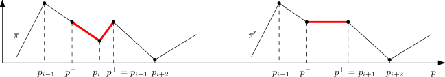
Figure 3: The removal of the vertex $\pi(p_{i})$ from $\pi$. The curve $\pi[p^{-},p^{+}]$ is marked red

In the construction of $f^{\prime}$ we need to show that the subcurve $\tau[f(p^{-}),f(p^{+})]$, which was matched by $f^{-1}$ to the missing part, can be matched to some subcurve of $\pi^{\prime}$, while respecting the monotonicity of the matching. The proof is a case analysis based on the structure of the two curves. In order to focus on the essential arguments, we first make some global assumptions stated below. The first two assumptions can be made without loss of generality. We also introduce some basic notation which is used throughout the rest of the proof.

Assumption 1.

We assume that $\pi(p_{i})$ is a local minimum on $\pi$ (otherwise we first mirror the curves $\tau$ and $\pi$ across the horizontal time axis to obtain this property without changing the Fréchet distance).

Let $z_{\min}=\operatorname*{arg\,min}_{t\in[f(p^{-}),f(p^{+})]}\tau(t)$. Let $\tau[s_{j},s_{j+1}]$ be the subcurve of $\tau$ bounded by two consecutive signature vertices, such that $z_{\min}\in[s_{j},s_{j+1}]$.

Assumption 2.

We assume that $\tau(s_{j})<\tau(s_{j+1})$ (otherwise we first reparametrize the curves $\tau$ and $\pi$ with $\phi(t)=1-t$, i.e., reverse the direction of the time axis, to obtain this property without changing the Fréchet distance; note that this does not change the property of $\pi(p_{i})$ being a local minimum).

Assumption 3.

We assume that neither $s_{j}=0$, nor $s_{j+1}=1$ (These are boundary cases which will be handled at the end of the proof).

Property 1 (Signature).

By Definition 3.3 we can assume that

1. $\tau(s_{j+1})-\tau(s_{j})>2\delta$,

2. $\tau(s_{j})=\min(\tau[s_{j-1},s_{j+1}])$,

3. $\tau(s_{j+1})=\max(\tau[s_{j},s_{j+2}])$,

4. $\tau(t)\geq\tau(t^{\prime})-2\delta$ for $s_{j}\leq t^{\prime}<t\leq s_{j+1}$.

5. $\tau(s_{j+1})-\tau(s_{j+2})>2\delta$,

By the general position assumption the minimum $\tau(s_{j})$ and the maximum $\tau(s_{j+1})$ are unique on their respective subcurves.

Property 2 (Fréchet).

Any two points matched by $f$ have distance at most $\delta$ from each other. In particular, for any two $0\leq p^{\prime}<p\leq 1$, it holds that

1. $\tau(f(p))-\delta\leq\pi(p)\leq\tau(f(p))+\delta$,

2. $\min(\tau[f(p^{\prime}),f(p)])-\delta\leq\min(\pi[p^{\prime},p])\leq\min(\tau[f(p^{\prime}),f(p)])+\delta$,

3. $\max(\tau[f(p^{\prime}),f(p)])-\delta\leq\max(\pi[p^{\prime},p])\leq\max(\tau[f(p^{\prime}),f(p)])+\delta$.

Our proof is structured as case analysis. We consider first the case $\tau(z_{\min})\geq\pi(p^{-})-\delta$. This is illustrated by Figure 4.

Case 1 (Trivial case).

$\tau(z_{\min})\geq\pi(p^{-})-\delta$

Figure 4: Example of Case 1. The broken part of the matching $f$ is indicated by fat lines.

Proof of Case 1.

As a warm-up exercise we quickly check that the above case is indeed trivial. In this case, we would simply match $\pi(p^{-})$ to the subcurve $\tau[f(p^{-}),f(p^{+})]$ and the remaining subcurves $\pi[0,p^{-}]$ and $\pi[p^{+},1]$ can be matched as done by $f$. Indeed,

$$\left\{{\tau(t)~{}|~{}t\in[f(p^{-}),f(p^{+})]}\right\}\subseteq[\pi(p^{-})]_{\delta},$$

since by the case distinction

$$\min(\tau[f(p^{-}),f(p^{+})])=\tau(z_{\min})\geq\pi(p^{-})-\delta$$

and by Property 2,

$$\max(\tau[f(p^{-}),f(p^{+})])\leq\max(\pi[p^{-},p^{+}])+\delta=\pi(p^{-})+\delta.$$

∎

Assumption 4.

We assume in the rest of the proof that $\tau(z_{\min})<\pi(p^{-})-\delta$ (non-trivial case).

Intuitively, we want to extend the subcurves of the trivial case in order to fix the broken matching. The difficulty lies in finding suitable subcurves which cover the broken part $\tau[f(p^{-}),f(p^{+})]$ and whose Fréchet distance is at most $\delta$. Furthermore, the endpoints need to line up suitably such that we can re-use $f$ for the suffix and prefix curves.

The next two claims settle the question, to which extent signature vertices can be included in the subcurve $\tau[f(p^{-}),f(p^{+})]$ for which we need to fix the broken matching.

Claim 3.9.

If $s_{j+1}\in[f(p^{-}),f(p^{+})]$ then $\left\{{\tau(t)~{}|~{}t\in[s_{j+1},f(p^{+})]}\right\}\subseteq[\tau(s_{j+1})-2\delta,\tau(s_{j+1})]$.

Proof.

We have to prove that

$$\min(\tau[s_{j+1},f(p^{+})])\geq\tau(s_{j+1})-2\delta\text{ and }\max(\tau[s_{j+1},f(p^{+})])\leq\tau(s_{j+1}).$$

The subcurve $\pi[p^{-},p^{+}]$ consists of two edges $\overline{\pi(p^{-})\pi(p_{i})}$ and $\overline{\pi(p_{i})\pi(p^{+})}$ and $\pi(p_{i})$ is the minimum of the subcurve. For the lower bound we distinguish two cases: $p_{i}\leq f^{-1}(s_{j+1})\leq p^{+}$ and $p^{-}\leq f^{-1}(s_{j+1})<p_{i}$.

If $p_{i}\leq f^{-1}(s_{j+1})\leq p^{+}$, then by Property 2

$$\min(\tau[s_{j+1},f(p^{+})])\geq\min(\pi[f^{-1}(s_{j+1}),p^{+}])-\delta=\pi(f^{-1}(s_{j+1}))-\delta\geq\tau(s_{j+1})-2\delta.$$

If $p^{-}\leq f^{-1}(s_{j+1})<p_{i}$, then since $z_{\min}<s_{j+1}$ it holds that

$$\tau(z_{\min})=\min(\tau[f(p^{-}),s_{j+1}])\geq\min(\pi[p^{-},f^{-1}(s_{j+1})])-\delta=\pi(f^{-1}(s_{j+1}))-\delta\geq\tau(s_{j+1})-2\delta.$$

It follows that

$$\min(\tau[s_{j+1},f(p^{+})])\geq\min(\tau[f(p^{-}),f(p^{+})])=\tau(z_{\min})\geq\tau(s_{j+1})-2\delta$$

as claimed.

Furthermore, by Property 1(v) it follows that

$$\min(\tau[s_{j+1},f(p^{+})])\geq\tau(s_{j+1})-2\delta>\tau(s_{j+2}),$$

and therefore $s_{j+2}\notin[f(p^{-}),f(p^{+})]$.

Now, Property 1(iii) implies the upper bound: $\max(\tau[s_{j+1},f(p^{+})])\leq\tau(s_{j+1}).$

∎

Claim 3.10.

$s_{j}\notin[f(p^{-}),f(p^{+})]$

Proof.

For the sake of contradiction, assume the claim is false, i.e. $s_{j}\in[f(p^{-}),f(p^{+})]$. We have (by definition)

$$z_{\min}\in[f(p^{-}),f(p^{+})]\cap[s_{j},s_{j+1}]$$

Furthermore, by definition $\tau(z_{\min})=\min(\tau[f(p^{-}),f(p^{+})])$, and by Property 1(ii), we have $\tau(s_{j})=\min(\tau[s_{j-1},s_{j+1}])$. This would imply that

$$\tau(z_{\min})=\min\left\{{\tau(t)~{}|~{}t\in[f(p^{-}),f(p^{+})]\cap[s_{j},s_{j+1}]}\right\}=\tau(s_{j}).$$

By the theorem statement $\pi(p_{i})\notin[\tau(s_{j})]_{\delta}=[\tau(z_{\min})]_{\delta}$. However, by Property 2,

$$\pi(p_{i})=\min(\pi[p^{-},p^{+}])\in[\min(\tau[f(p^{-}),f(p^{+})])]_{\delta}=[\tau(z_{\min})]_{\delta}.$$

∎

We now introduce some more notation which will be used throughout the proof.

$$t_{\min} = \operatorname*{arg\,min}_{t\in[f(p^{-}),s_{j+1}]}\tau(t)$$

$$x = \max\{p\in[0,p^{-}]~{}|~{}\pi(p)=\min(\tau(t_{\min})+\delta,\tau(s_{j+1})-\delta)\}$$

$$p_{\max} = \operatorname*{arg\,max}_{p\in[x,p^{-}]}\pi(p)$$

$$y = \min\{t\in[t_{\min},1]~{}|~{}\tau(t)=\pi(p_{\max})-\delta\}$$

In the next few claims we argue that these variables are well-defined. In particular, that $x$ and $y$ always exist in the non-trivial case (Claim 3.11 and Claim 3.12). Clearly $t_{\min}$ is well-defined and by our initial assumptions we have $z_{\min}\leq t_{\min}$ (since $z_{\min}\in[s_{j},s_{j+1}]$). We also derive some bounds along the way, which will be used throughout the later parts of the proof.

Claim 3.11 (Existence of $x$).

It holds that

1. $\min(\tau(t_{\min})+\delta,\tau(s_{j+1})-\delta)\in\{\pi(p)~{}|~{}p\in[f^{-1}(s_{j}),p^{-}]\}$

2. $\min(\pi[x,p^{-}])\geq\min(\tau(t_{\min})+\delta,\tau(s_{j+1})-\delta)=\pi(x)$

3. $\tau(s_{j})<\tau(t_{\min})$

Proof.

We first prove part (i) of the claim. We show that there exist two parameters $f^{-1}(s_{j})\leq p_{1}\leq p_{2}\leq p^{-}$ such that

$$\pi(p_{1})\leq\min\!\left({\tau(t_{\min})+\delta,\tau(s_{j+1})-\delta}\right)\leq\pi(p_{2}).$$

Since the curve is continuous, this would imply the claim. Indeed, we can choose $p_{1}=f^{-1}(s_{j})$ and $p_{2}=p^{-}$. If $s_{j+1}\geq f(p^{+})$ we have

$$\pi(p_{2})=\pi(p^{-})\geq\tau(z_{\min})+\delta\geq\tau(t_{\min})+\delta,$$

(since we assume the non-trivial case). Otherwise, if $s_{j+1}<f(p^{+})$ and therefore $\tau(s_{j+1})=\max(\tau[f(p^{-}),f(p^{+})])$, then by Property 1 and Property 2,

$$\pi(p_{2})=\pi(p^{-})=\max(\pi[p^{-},p^{+}])\geq\max(\tau[f(p^{-}),f(p^{+})])-\delta=\tau(s_{j+1})-\delta.$$

Thus, in both cases, it holds that $\pi(p_{2})\geq\min\!\left({\tau(t_{\min})+\delta,\tau(s_{j+1})-\delta}\right)$.

As for $p_{1}$, by Claim 3.10 we have $0\leq s_{j}\leq f(p^{-})\leq t_{\min}\leq s_{j+1}$ and by Property 2

$$\pi(p_{1})=\pi(f^{-1}(s_{j}))\leq\tau(s_{j})+\delta.$$

It follows by Property 1(ii) that $\pi(p_{1})<\tau(t_{\min})+\delta$ and by Property 1(i) that $\pi(p_{1})<\tau(s_{j+1})-\delta.$ Now, part (ii) of the claim follows directly from the above, since $\pi(x)$ is defined as the last point along the prefix subcurve $\pi[0,p^{-}]$ with the specified value and since $\pi(x)\leq\pi(p^{-})$. Note that part (iii) we indirectly proved above. ∎

Claim 3.12 (Existence of $y$).

It holds that

1. $\pi(p_{\max})-\delta\in\{\tau(t)~{}|~{}t\in[t_{\min},s_{j+1}]\}$

2. $\max(\tau[t_{\min},y])\leq\pi(p_{\max})-\delta=\tau(y)$

3. $\pi(p_{\max})<\tau(s_{j+1})+\delta$

Proof.

To prove part (i) of the claim we show that there exist two parameters $t_{\min}\leq t_{1}\leq t_{2}\leq s_{j+1}$, such that

$$\tau(t_{1})\leq\pi(p_{\max})-\delta\leq\tau(t_{2}).$$

We choose $t_{1}=t_{\min}$ and $t_{2}=s_{j+1}$. Since we have the non-trivial case, we know

$$\pi(p_{\max})\geq\pi(p^{-})\geq\tau(z_{\min})+\delta\geq\tau(t_{\min})+\delta=\tau(t_{1})+\delta.$$

Now, for $t_{2}$, we know that $s_{j}\leq f(x)\leq f(p_{\max})\leq f(p^{-})\leq s_{j+1}$. By Property 2 and by Property 1(iii)

$$\tau(t_{2})=\tau(s_{j+1})\geq\tau(f(p_{\max}))\geq\pi(p_{\max})-\delta.$$

Since the subcurve is continuous, there must be a parameter $t_{1}\leq t\leq t_{2}$ which satisfies the claim. Now, part (ii) of the claim also follows directly, since $\tau(y)$ is the first point along the suffix subcurve $\tau[t_{\min},1]$ with the specified value and since $\tau(y)\geq\tau(t_{\min})$. Note that part (iii) we just proved above. ∎

The following claim follows directly from Claim 3.11 and Claim 3.12.

Claim 3.13.

$s_{j}\leq f(x)\leq y\leq s_{j+1}$

The following claim will be used throughout the proof.

Claim 3.14.

$\pi(p_{\max})-2\delta\leq\pi(x)$

Proof.

We need to show that

$$\pi(p_{\max})-2\delta\leq\min(\tau(t_{\min})+\delta,\tau(s_{j+1})-\delta)$$

Claim 3.12 immediately implies $\pi(p_{\max})\leq\tau(s_{j+1})+\delta$. On the other hand, by Claim 3.13,

$$s_{j}\leq f(x)\leq f(p_{\max})\leq f(p^{-})\leq t_{\min}\leq s_{j+1}.$$

By Property 2 and by Property 1(iv),

$$\pi(p_{\max})\leq\tau(f(p_{\max}))+\delta\leq\tau(t_{\min})+3\delta$$

∎

The next two claims (Claim 3.15 and Claim 3.16) show that our choice of $x$ and $y$ is suitable for fixing some part of the broken matching: the subcurve $\pi[x,p^{-}]$ can be matched entirely to $\tau(y)$ and the subcurve $\tau[f(x),y]$ can be matched entirely to $\pi(x)$. After that, it remains to match the subcurve $\pi[p^{+},f^{-1}(y)]$. For this we have the case analysis that follows.

Claim 3.15.

$\left\{{\pi(p)~{}|~{}p\in[x,p^{-}]}\right\}\subseteq[\pi(p_{\max})-2\delta,\pi(p_{\max})]=[\tau(y)]_{\delta}.$

Proof.

By Claim 3.11 and Claim 3.14,

$$\min(\pi[x,p^{-}])\geq\min\!\left({\tau(t_{\min})+\delta,\tau(s_{j+1})-\delta}\right)\geq\pi(p_{\max})-2\delta.$$

On the other hand, by definition of $p_{\max}$, we have $\max(\pi[x,p^{-}])=\pi(p_{\max}).$ The last equality of the claim follows directly from the definition of $y$ and from Claim 3.12 ($y$ is well-defined). ∎

Claim 3.16.

$\left\{{\tau(t)~{}|~{}t\in[f(x),y]}\right\}\subseteq[\min\!\left({\tau(t_{\min})+\delta,\tau(s_{j+1})-\delta}\right)]_{\delta}=[\pi(x)]_{\delta}.$

Proof.

We first prove the lower bound on the minimum of the subcurve $\tau[f(x),y]$. By Claim 3.11, and by Property 2, we have

$$\min(\tau[f(x),f(p^{-})])\geq\min(\pi[x,p^{-}])-\delta\geq\min\!\left({\tau(t_{\min}),\tau(s_{j+1})-2\delta}\right).$$

By definition, $\tau(t_{\min})$ is a minimum on $\tau[f(p^{-}),s_{j+1}]$, thus

$$\min(\tau[f(p^{-}),y])\geq\tau(t_{\min})\geq\min\!\left({\tau(t_{\min}),\tau(s_{j+1})-2\delta}\right),$$

for $y\leq s_{j+1}$, which is ensured by Claim 3.13.

We now prove the upper bound on the maximum of the subcurve $\tau[f(x),y]$. Since by Claim 3.12 $s_{j}\leq f(x)\leq t_{\min}\leq s_{j+1}$ and since by Property 1(iv), $\tau[s_{j},s_{j+1}]$ may not descend by more than $2\delta$, it follows that

$$\max(\tau[f(x),t_{\min}])\leq\tau(t_{\min})+2\delta.$$

By definitions of $x$ and $y$ and by Claim 3.14

$$\max(\tau[t_{\min},y])\leq\pi(p_{\max})-\delta\leq\pi(x)+\delta\leq\tau(t_{\min})+2\delta.$$

By Property 1(iii) we also have,

$$\max(\tau[f(x),y])\leq\tau(s_{j+1}),$$

for $y\leq s_{j+1}$, which is ensured by Claim 3.13.

Together this implies the claim. The last equality of the claim follows directly from the definition of $x$ and from Claim 3.11 ($x$ is well-defined). ∎

Now we have established the basic setup for our proof. In the following, we describe the case analysis based on the structure of the two curves $\tau$ and $\pi$. Consider walking along the subcurve $\pi[p^{+},1]$. At the beginning of the subcurve, we have $\pi(p^{+})\in[\pi(x),\pi(p_{\max})]$. One of the following events may happen during the walk: either we go above $\pi(p_{\max})$, or we go below $\pi(x)$, or we stay inside this interval. Let $q$ denote the time at which for the first time one of these events happens. Formally, we define the intersection function $g:{\rm I\!R}\rightarrow[p^{+},1]\cup\left\{{p_{\infty}}\right\}$,

$$g(h) = \min(\{p\in[p^{+},1]~{}|~{}\pi(p)=h\}\cup\{p_{\infty}\})$$

$$q = \min\!\left({g(\pi(p_{\max})),g(\pi(x))}\right),$$

where $p_{\infty}>1$ is some fixed constant for the case that the suffix curve $\pi[p^{+},1]$ does not contain the value $h$. We distinguish the following main cases. In each of the cases, we devise a matching scheme to fix the broken matching. For each case, our construction ensures that the extended subcurves cover the subcurve $\tau[f(p^{-}),f(p^{+})]$ and that the subcurves line up with suitable prefix and suffix curves, such that we can always use $f$ for the parts of $\pi$ and $\tau$ not covered in the matching scheme. We need to prove in each case that the Fréchet distance between the specified subcurves is at most $\delta$. If this is the case, we call the matching scheme valid.

We have to make further distinction between the case when $f(p^{+})\leq y$ and the case $f(p^{+})>y$. If $f(p^{+})\leq y$ holds, the three aforementioned events are described by Case 2, Case 3 and Case 4. If it happens that $f(p^{+})>y$, it becomes more complicated to repair the matching. This is discussed in Case 5.

Case 2 ($\pi$ stays level).

$p^{+}\leq f^{-1}(y)\leq q$.

Figure 5: Example of Case 2. The broken part of the matching $f$ is indicated by fat lines.

Case 2 is the simplest case. We intend to use the following matching scheme:

$$\pi(x) \Leftrightarrow \tau[f(x),y]$$

$$\pi[x,p^{-}] \Leftrightarrow \tau(y)$$

$$\pi[p^{+},f^{-1}(y)] \Leftrightarrow \tau(y)$$

Proof of Case 2.

Claim 3.16 implies that the Fréchet distance between $\tau[f(x),y]$ and $\pi(x)$ is at most $\delta$. Claim 3.15 implies that the Fréchet distance between $\pi[x,p^{-}]$ and $\tau(y)$ is at most $\delta$. Finally, by our case distinction and by Claim 3.14

$$\left\{{\pi(p)~{}|~{}p\in[p^{+},f^{-1}(y)]}\right\}\subseteq[\pi(x),\pi(p_{\max})]\subseteq[\pi(p_{\max})-2\delta,\pi(p_{\max})]=[\tau(y)]_{\delta}.$$

Therefore, also the Fréchet distance between $\pi[p^{+},f^{-1}(y)]$ and $\tau(y)$ is at most $\delta$. ∎

Case 3 ($\pi$ tends upwards).

$q<f^{-1}(y)$ and $q=g(\pi(p_{\max}))$

Figure 6: Example of Case 3. The broken part of the matching $f$ is indicated by fat lines.

In Case 3, let $y^{\prime}=\max\{t\in[0,f(q)]~{}|~{}\tau(t)=\tau(y)\}$ and $z=\max\{p^{+},f^{-1}(y^{\prime})\}$. We intend to use the following matching scheme:

$$\pi(x) \Leftrightarrow \tau[f(x),y^{\prime}]$$

$$\pi[x,p^{-}] \Leftrightarrow \tau(y^{\prime})$$

$$\pi[p^{+},z] \Leftrightarrow \tau(y^{\prime})$$

$$\pi(z) \Leftrightarrow \tau[y^{\prime},f(p^{+})]$$

(Note that if $y^{\prime}>f(p^{+})$, then the last line of the above matching scheme is simply dropped.)

Proof of Case 3.

We first argue that $y^{\prime}$ exists. To this end, we show that there exist two parameters $0\leq t_{1}<t_{2}\leq f(q)$, such that

$$\tau(t_{1})\leq\tau(y)=\pi(p_{\max})-\delta\leq\tau(t_{2}).$$

We choose $t_{1}=z_{\min}$ and $t_{2}=f(q)$. Note that $z_{\min}\leq f(p^{+})\leq f(q)$. Now, by Property 2,

$$\tau(t_{2})=\tau(f(q))\geq\pi(q)-\delta=\pi(p_{\max})-\delta.$$

Since we are assuming the non-trivial case,

$$\pi(p_{\max})\geq\pi(p^{-})\geq\tau(z_{\min})+\delta=\tau(t_{1})+\delta.$$

Thus, since $\tau[0,f(q)]$ is continuous, $y^{\prime}$ must exist and it holds that $f(p^{-})\leq z_{\min}\leq y^{\prime}$. It remains to prove that the matching scheme is valid. Since $y^{\prime}\leq f(q)<y$, Claim 3.16 implies that the Fréchet distance between $\tau[f(x),y^{\prime}]$ and $\pi(x)$ is at most $\delta$. Claim 3.15 implies that the Fréchet distance between $\pi[x,p^{-}]$ and $\tau(y^{\prime})$ is at most $\delta$. For the last two lines of the matching scheme we distinguish two cases. If $y^{\prime}>f(p^{+})$, then $z=f^{-1}(y^{\prime})$ and we need to prove that

$$\left\{{\pi(p)~{}|~{}p\in[p^{+},f^{-1}(y^{\prime})]}\right\}\subseteq[\tau(y^{\prime})]_{\delta}.$$

By our case distinction and by Claim 3.14

$$\left\{{\pi(p)~{}|~{}p\in[p^{+},q]}\right\}\subseteq[\pi(x),\pi(p_{\max})]\subseteq[\pi(p_{\max})-2\delta,\pi(p_{\max})]=[\tau(y^{\prime})]_{\delta}.$$

Since $f^{-1}(y^{\prime})\leq q$, this implies the validity of the matching. Otherwise, if $y^{\prime}\leq f(p^{+})$, then $z=p^{+}$ and we need to prove that

$$\left\{{\tau(t)~{}|~{}t\in[y^{\prime},f(p^{+})]}\right\}\subseteq[\pi(p^{+})]_{\delta}.$$

This can be derived as follows. On the one hand, by Property 2, since $y^{\prime}\in[f(p^{-}),f(p^{+})]$

$$\max(\tau[y^{\prime},f(p^{+})])\leq\max(\pi[f^{-1}(y^{\prime}),p^{+}])+\delta=\max(\pi[p^{-},p^{+}])+\delta=\pi(p^{+})+\delta.$$

On the other hand, by the definition of $y^{\prime}$ and since $y^{\prime}\leq f(p^{+})\leq f(q)$

$$\min(\tau[y^{\prime},f(p^{+})])=\tau(y^{\prime})=\pi(p_{\max})-\delta\geq\pi(p^{+})-\delta.$$

∎

Case 4 ($\pi$ tends downwards).

$q<f^{-1}(y)$ and $q=g(\pi(x))$.

Figure 7: Example of Case 4. The broken part of the matching $f$ is indicated by fat lines.

In Case 4, let $y^{\prime\prime}=\min\{t\in[f(p_{\max}),1]~{}|~{}\tau(t)=\tau(y)\}$. We intend to use the following matching scheme:

$$\pi(p_{\max}) \Leftrightarrow \tau[f(p_{\max}),y^{\prime\prime}]$$

$$\pi[p_{\max},p^{-}] \Leftrightarrow \tau(y^{\prime\prime})$$

$$\pi[p^{+},q] \Leftrightarrow \tau(y^{\prime\prime})$$

$$\pi(q) \Leftrightarrow \tau[y^{\prime\prime},f(q)]$$

Proof of Case 4.

Clearly, $y^{\prime\prime}$ exists in the non-trivial case, since

$$\tau(f(p_{\max}))\geq\tau(y)\geq\tau(z_{\min}),$$

and $f(p_{\max})\leq f(p^{-})\leq z_{\min}$.

We prove the validity of the matching scheme line by line. Note that by definition $\tau(y^{\prime\prime})=\tau(y)=\pi(p_{\max})-\delta$. For the first matching: by the definition of $y^{\prime\prime}$ and by Property 2,

$$\left\{{\tau(t)~{}|~{}t\in[f(p_{\max}),y^{\prime\prime}]}\right\}\subseteq[\pi(p_{\max})]_{\delta}.$$

The validity of the second matching follows from Claim 3.15 since $p_{\max}\geq x$. For the third matching: By our case distinction and by Claim 3.14

$$\left\{{\pi(t)~{}|~{}t\in[p^{+},q]}\right\}\subseteq[\pi(x),\pi(p_{\max})]\subseteq[\pi(p_{\max})-2\delta,\pi(p_{\max})]=[\tau(y^{\prime\prime})]_{\delta}.$$

As for the last matching, since $f(x)\leq f(p_{\max})\leq y^{\prime\prime}$ and since by our case distinction $f(q)<y$, Claim 3.16 implies

$$\left\{{\tau(t)~{}|~{}t\in[y^{\prime\prime},f(q)]}\right\}\subseteq[\pi(x)]_{\delta}=[\pi(q)]_{\delta}.$$

∎

Case 5 (The matroska case).

$f(p^{+})>y$.

Case 5 seems to be the most difficult case to handle. However, we have already established a suitable set of tools in the previous cases. We devise an iterative matching scheme and prove an invariant (Claim 3.17) to verify that the Fréchet distance of the subcurves is at most $\delta$. We first define $z_{\min}^{(1)}=z_{\min}$, $t_{\min}^{(1)}=t_{\min}$, $x^{(1)}=x$, and $y^{(1)}=y$. Now, for $a=2,\dots$ let

$$z_{\min}^{(a)} = \operatorname*{arg\,min}_{t\in[y^{(a-1)},f(p^{+})]}\tau(t)$$

$$t_{\min}^{(a)} = \operatorname*{arg\,min}_{t\in[y^{(a-1)},s_{j+1}]}\tau(t)$$

$$x^{(a)} = \min\left\{{p\in[x^{(a-1)},p_{\max}]~{}|~{}\pi(p)=\min\!\left({\tau(t_{\min}^{(a)})+\delta,\tau(s_{j+1})-\delta}\right)}\right\}$$

$$y^{(a)} = \min\{t\in[t_{\min}^{(a)},s_{j+1}]~{}|~{}\tau(t)=\pi(p_{\max})-\delta\},$$

We describe the intended matching scheme, beginning with the following subcurves:

$$\pi(x^{(1)}) \Leftrightarrow \tau[f(x^{(1)}),y^{(1)}]$$

$$\pi[x^{(a-1)},x^{(a)}] \Leftrightarrow \tau(y^{(a-1)})$$

$$\pi(x^{(a)}) \Leftrightarrow \tau[y^{(a-1)},y^{(a)}],$$

where the last two matchings are repeated while incrementing $a$ (starting with $a=2$). After each iteration, we are left with the unmatched subcurves $\pi[x^{(a)},p^{-}]$ and $\tau[y^{(a)},f(p^{+})]$. We would like to complete the matching with the following scheme

$$\pi[x^{(a)},p^{-}] \Leftrightarrow \tau(y^{(a)})$$

$$\pi(p^{+}) \Leftrightarrow \tau[y^{(a)},f(p^{+})]$$

This is indeed possible if

$$\pi(p^{-})\leq\tau(z_{\min}^{(a+1)})+\delta.$$

The above is the equivalent to the trivial case (Case 1). We first prove correctness in this case (Case 5(i)). To this end, we extend Claim 3.16 as follows. Note that this claim will also be used in the non-trivial cases that follow.

Claim 3.17.

$\left\{{\tau(t)~{}|~{}t\in[y^{(a-1)},y^{(a)}]}\right\}\subseteq\left[{\tau(t_{\min}^{(a)})~{},~{}\min(\tau(t_{\min}^{(a)})+2\delta,\tau(s_{j+1}))}\right]\subseteq[\pi(x^{(a)})]_{\delta}.$

Proof.

Recall that $s_{j}\leq y\leq y^{(a-1)}\leq y^{(a)}\leq s_{j+1}$ by Claim 3.13. By definition of $t_{\min}^{(a)}$,

$$\min(\tau[y^{(a-1)},y^{(a)}])\geq\min(\tau[y^{(a-1)},s_{j+1}])\geq\tau(t_{\min}^{(a)}).$$

By Property 1(iv) and the definitions of $y^{(a)}$ and $t_{\min}^{(a)}$, we also have that

$$\max(\tau[y^{(a-1)},y^{(a)}])\leq\tau(t_{\min}^{(a)})+2\delta,$$

and by Property 1(iii), we also have that

$$\max(\tau[y^{(a-1)},y^{(a)}])\leq\tau(s_{j+1}).$$

This proves the first part of the claim. For the second part we use the definition of $\pi(x^{(a)})=\min(\tau(t_{\min}^{(a)})+\delta,\tau(s_{j+1})-\delta)$, which implies

$$\tau(t_{\min}^{(a)}) \geq \pi(x^{(a)})-\delta$$

$$\min(\tau(t_{\min}^{(a)})+2\delta,\tau(s_{j+1})) = \pi(x^{(a)})+\delta.$$

∎

Claim 3.18 (Correctness of Case 5(i)).

If for some value of $a$, it holds that $\pi(p^{-})\leq\tau(z_{\min}^{(a+1)})+\delta$ then the above matching scheme is valid.

Proof.

By Claim 3.16, Claim 3.15 and Claim 3.17 the iterative part of the matching scheme is valid. It remains to prove the validity of the last two matchings. By Claim 3.15,

$$\left\{{\pi(p)~{}|~{}p\in[x,p^{-}]}\right\}\subseteq[\pi(p_{\max})-2\delta,\pi(p_{\max})]=[\tau(y)]_{\delta}=[\tau(y^{(a)})]_{\delta}.$$

Since $x\leq x^{(a)}\leq p^{-}$, this implies that the Fréchet distance between $\pi[x^{(a)},p^{-}]$ and $\tau(y^{(a)})$ is at most $\delta$. As for the other matching, we have by our case distinction

$$\pi(p^{-})\leq\tau(z_{\min}^{(a+1)})+\delta=\min(\tau[y^{(a)},f(p^{+})])+\delta,$$

while (by Property 2) the matching $f$ testifies that

$$\max(\tau[f(p^{-}),f(p^{+})])\leq\max(\pi[p^{-},p^{+}])+\delta=\pi(p^{-})+\delta.$$

Since $f(p^{+})\geq y^{(a)}\geq y\geq f(p^{-})$, the above implies

$$\left\{{\tau(t)~{}|~{}t\in[y^{(a)},f(p^{+})]}\right\}\subseteq[\pi(p^{-})]_{\delta}=[\pi(p^{+})]_{\delta}.$$

Note that the proof holds both if $s_{j+1}<f(p^{+})$ or $s_{j+1}\geq f(p^{+})$. ∎

From now on, we will assume the non-trivial (sub)case. Our matching scheme is based on a stopping parameter $\overline{a}$, which (intuitively) depends on whether $f$ matched some point on the missing subcurve $\pi[p^{-},p^{+}]$ to a signature vertex $\tau(s_{j+1})$ of $\tau$.

Definition 3.19.

(Stopping parameter $\overline{a}$) If $s_{j+1}\geq f(p^{+})$ then let $\overline{a}$ be the minimal value of $a$ satisfying $f(p^{+})\leq y^{(a)}.$ Otherwise, let $\overline{a}$ be the minimal value of $a$ such that $y^{(a)}=y^{(a+1)}\leq s_{j+1}.$

Claim 3.20.

The stopping parameter $\overline{a}$ (Definition 3.19) is well-defined and the matching scheme is valid for $a\leq\overline{a}.$

Proof.

We first argue that there must be a value of $a$ such that $t_{\min}^{(a+1)}=y^{(a)}=y^{(b)}$ for any $b>a$. Recall that by our initial assumptions, $z_{\min}\in[s_{j},s_{j+1}]$ and thus $z_{\min}\leq t_{\min}\leq s_{j+1}$. As a consequence, Claim 3.12 testifies that in the non-trivial case, the point $\tau(y)$ exists and is well-defined. We defined $y^{(1)}=y$ and for $a>1$ we defined

$$y^{(a)}=\min\{t\in[t_{\min}^{(a)},s_{j+1}]~{}|~{}\tau(t)=\pi(p_{\max})-\delta\}.$$

Since by Claim 3.12, $\tau(s_{j+1})\geq\pi(p_{\max})-\delta=\tau(y^{(a)})$, there must be a value of $a$ such that

$$\min(\tau[y^{(a)},s_{j+1}])\geq\tau(y^{(a)}).$$

Let this value of $a$ be denoted $\widehat{a}$. In this case, it follows by definition that $t_{\min}^{(\widehat{a}+1)}=y^{(\widehat{a})}$, which implies that $y^{(\widehat{a}+1)}=y^{(\widehat{a})}$ and $t_{\min}^{(\widehat{a}+2)}=y^{(\widehat{a}+1)},\dots$. This has the effect that $y^{(\widehat{a})}=y^{(b)}$ for any $b>\widehat{a}$.

Now, if $s_{j+1}<f(p^{+})$, then the above analysis implies that $\overline{a}$ is well-defined. However, if $s_{j+1}\geq f(p^{+})$, we defined $\overline{a}$ to be the minimal value of $a$ such that $f(p^{+})\leq y^{(a)}$. Now it might happen that $y^{(\widehat{a})}\leq f(p^{+})\leq s_{j+1}$. In this case, there exists no value of $a$ such that $f(p^{+})\leq y^{(a)}$, thus $y^{(\overline{a})}$ does not exist. We can reduce this case to the trivial case (Case 5(i)) as follows. By Claim 3.12, $\tau(s_{j+1})\geq\pi(p_{\max})-\delta$ and by Property 1(iii), $\tau(s_{j+1})$ must be a maximum on $\tau[s_{j},s_{j+2}]$. Thus, by definition of $t_{\min}^{(\overline{a})}$, we would have $\tau\left(z_{\min}^{(\overline{a})}\right)=\tau\left(t_{\min}^{(\overline{a})}\right)=\tau(y^{(\overline{a}-1)})=\pi(p_{\max})-\delta\geq\pi(p^{-})-\delta$, which is Case 5(i) (the trivial case). Thus, also in the non-trivial case, $\overline{a}$ is well-defined.

The validity of the matching scheme for $a\leq\overline{a}$ follows from Claim 3.16, Claim 3.15 and Claim 3.17. ∎

It follows that the iterative part of the matching scheme is valid for $a\leq\overline{a}.$ Now we are left with the unmatched subcurves $\pi[x^{(\overline{a})},p^{-}]$ and $\tau[y^{(\overline{a})},f(p^{+})]$ and we have to complete the matching scheme. In order to set up a case analysis with a similar structure as before, we define

$$q^{\prime} = \min\!\left({g(\pi(p_{\max})),g(\tau(t_{\min}^{(\overline{a}-1)})+\delta)}\right)$$

$$q^{\prime\prime} = \min\!\left({g(\pi(p_{\max})),g(\tau(s_{j+1})-\delta)}\right)$$

case	definition	intended matching
5(i)	$\exists a:\pi(p^{-})\leq\tau(z_{\min}^{(a+1)})+\delta$	$\pi[x^{(a)},p^{-}]\Leftrightarrow\tau(y^{(a)})$ $\pi(p^{+})\Leftrightarrow\tau[y^{(a)},f(p^{+})]$
5(ii)	$p^{+}\leq f^{-1}(y^{(\overline{a})})\leq q^{\prime}$	$\pi[x^{(\overline{a})},p^{-}]\Leftrightarrow\tau(y^{\overline{a}})$ $\pi[p^{+},f^{-1}(y^{\overline{a}})]\Leftrightarrow\tau(y^{\overline{a}})$
5(iii)	$p^{+}\leq q^{\prime}<f^{-1}(y^{(\overline{a})})$ and $q^{\prime}=g(\pi(p_{\max}))$	This case can be reduced to Case 5(i)
5(iv)	$p^{+}\leq q^{\prime}<f^{-1}(y^{(\overline{a})})$ and $q^{\prime}=g(\tau(t_{\min}^{\overline{a}-1})+\delta)$	$\pi[x^{(\overline{a}-1)},p^{-}]\Leftrightarrow\tau(y^{(\overline{a}-1)})$ $\pi[p^{+},q^{\prime}]\Leftrightarrow\tau(y^{(\overline{a}-1)})$ $\pi(q^{\prime})\Leftrightarrow\tau[y^{(\overline{a}-1)},f(q^{\prime})]$
5(v)	$p^{+}>f^{-1}(y^{(\overline{a})})$ and $q^{\prime\prime}=g(\pi(p_{\max}))$ For the matching scheme, let $x^{\prime}=\min\{t\in[x^{(\overline{a})},p_{\max}]~{}|~{}\tau(t)=\tau(s_{j+1})-\delta\}$ $y^{\prime}=\max\{t\in[0,f(q)]~{}|~{}\tau(t)=\tau(y)\}$ $z=\max\{p^{+},f^{-1}(y^{\prime})\}$	$\pi[x^{(\overline{a})},x^{\prime}]\Leftrightarrow\tau(y^{(\overline{a})})$ $\pi(x^{\prime})\Leftrightarrow\tau[y^{(\overline{a})},y^{\prime}]$ $\pi[x^{\prime},p^{-}]\Leftrightarrow\tau(y^{\prime})$ $\pi[p^{+},z]\Leftrightarrow\tau(y^{\prime})$ $\pi[z]\Leftrightarrow\tau[y^{\prime},f(p^{+})]$
5(vi)	$p^{+}>f^{-1}(y^{(\overline{a})})$ and $q^{\prime\prime}=g(\tau(s_{j+1})-\delta)$	$\pi[x^{(\overline{a})},p^{-}]\Leftrightarrow\tau(y^{(\overline{a})})$ $\pi[p^{+},q^{\prime\prime}]\Leftrightarrow\tau(y^{(\overline{a})})$ $\pi(q^{\prime\prime})\Leftrightarrow\tau[y^{(\overline{a})},f(q^{\prime\prime})]$

Table 1: Subcases for Case 5: (i) trivial case (Claim 3.18), (ii) $\pi$ stays level, (iii) $\pi$ tends upwards, (iv) $\pi$ tends downwards, (v) unmatched signature vertex and $\pi$ tends upwards, (vi) unmatched signature vertex and $\pi$ tends downwards. Examples of these cases are shown in Figure 8 and Figure 9.

The exact case distinction is specified in Table 1: (i) trivial case (see Claim 3.18), (ii) $\pi$stays level, (iii) $\pi$tends upwards, (iv) $\pi$tends downwards, (v) unmatched signature vertex and $\pi$ tends upwards, (vi) unmatched signature vertex and $\pi$ tends downwards. It remains to prove that the case analysis is complete and to prove correctness in each of these subcases.

Claim 3.21.

The case distinction of subcases of Case 5 (Table 1) is complete.

Proof.

We assume that we are not in the trivial case Case 5(i). If $f(p^{+})\leq y^{(\overline{a})}$ (also $f(p^{+})\leq y^{(\overline{a})}\leq s_{j+1}$) we get one of Case 5(ii)-(iv). Otherwise we have $f(p^{+})>y^{(\overline{a})}$ (also $f(p^{+})>s_{j+1}\geq y^{(\overline{a})}$). In this case, we get one of Case 5(v)-(vi). In the following, we argue that, indeed, if the subcurve of $\tau$ specified by the parameter interval $[f(p^{-}),f(p^{+})]$ contains the signature vertex at $s_{j+1}$, it must be that

$$\tau(s_{j+1})-\delta\in\left\{{\pi(p)~{}|~{}p\in[p^{+},1]}\right\}$$

and thus, $q^{\prime\prime}\neq p_{\infty}$ and $\pi(q^{\prime\prime})$ is be one of $\left\{{\pi(p_{\max}),\tau(s_{j+1})-\delta}\right\}$. Assume that $s_{j+2}\neq 1$, i.e., the next signature vertex after $\tau(s_{j+1})$ is not the last signature vertex. In this case, by Property 1 and Property 2, we have

$$\tau(s_{j+1})\geq\tau(s_{j+2})+2\delta\geq\pi(f^{-1}(s_{j+2}))+\delta.$$

Since $\pi$ is continuous, this implies that there must exist a point $\pi(t)$ with $t\geq p^{+}$ and $\pi(t)\leq\tau(s_{j+1})-\delta$. Now, assume that $s_{j+2}=1$. In this case, we have by the theorem statement that $\pi(p_{i})\notin[\tau(s_{j+2})]_{4\delta}$. It must be that either $\tau(s_{j+1})\geq\pi(p_{i})>\tau(s_{j+2})+4\delta$ (in which case we can apply the above argument), or $\pi(p_{i})<\tau(s_{j+2})-4\delta\leq\tau(s_{j+1})-5\delta$. The second case is not possible since by Claim 3.14 and by Property 2 we have

$$\pi(p_{i}) \geq \tau(f(p_{i}))-\delta\geq\tau(t_{\min})-\delta\geq\pi(p_{\max})-4\delta$$

$$\geq\pi(p^{+})-4\delta\geq\pi(f^{-1}(s_{j+1}))-4\delta\geq\tau(s_{j+1})-5\delta.$$

Here, $\pi(p^{+})\geq\pi(f^{-1}(s_{j+1}))$ follows from $s_{j+1}\in[f(p^{-}),f(p^{+})]$ in Case 5(v)-(vi) and the fact that

$$\max(\pi[p^{-},p^{+}])=\pi(p^{+}),$$

by our initial assumptions. ∎

Proof of Case 5(ii).

By Claim 3.15 the Fréchet distance between $\pi[x^{(\overline{a})},p^{-}]$ and $\tau(y^{(\overline{a})})$ is at most $\delta$. By our case distinction,

$$\left\{{\pi(p)~{}|~{}p\in[p^{+},f^{-1}(y^{(\overline{a})})]}\right\}\subseteq[\tau(t_{\min}^{(\overline{a}-1)})+\delta,\pi(p_{\max})]\subseteq[\pi(p_{\max})-2\delta,\pi(p_{\max})]=[\tau(y^{(\overline{a})})]_{\delta},$$

since by Claim 3.14,

$$\tau(t_{\min}^{(\overline{a}-1)})+\delta\geq\tau(t_{\min})+\delta\geq\pi(p_{\max})-2\delta.$$

(Note that $t_{\min}^{(\overline{a}-1)}$ always exists since $y^{(1)}\leq s_{j+1}$ by Claim 3.13.) This implies that also the second matching is valid. ∎

Proof of Case 5(iii).

We can reduce this case to Case 5(i) (the trivial case) as follows. By our case distinction, $f(p^{+})\leq f(q^{\prime})<y^{(\overline{a})}$. Let $b$ be the maximal value of $a$ such that $f(q^{\prime})\in[y^{(a)},y^{(\overline{a})}]$. By Property 2 it must be that $\tau(f(q^{\prime}))\geq\pi(p_{\max})-\delta=\tau(y^{(b)})$. Thus $\min(\tau[y^{(b)},f(q^{\prime})])\geq\pi(p_{\max})-\delta$. This holds since for any $a^{\prime}$, $\tau$ goes upwards in $\tau(y^{(a^{\prime})})$, then intersects $\pi(p_{\max})-\delta$ downwards and goes upwards again in $\tau(y^{(a^{\prime}+1)})$. By our case distinction, $f(p^{+})\in[y^{(b)},f(q^{\prime})]$. Thus,

$$\tau(z_{\min}^{(b+1)})=\min(\tau[y^{(b)},f(p^{+})])\geq\min(\tau[y^{(b)},f(q^{\prime})])\geq\pi(p_{\max})-\delta\geq\pi(p^{-})-\delta.$$

∎

Proof of Case 5(iv).

In this case, we rollback the last two matchings of the iterative matching scheme and instead end with $a=\overline{a}-1$. Thus, we are left with the unmatched subcurves $\pi[x^{(\overline{a}-1)},p^{-}]$ and $\tau[y^{(\overline{a}-1)},f(p^{+})]$. We complete the matching scheme as defined in Table 1. The validity of the first matching follows directly from Claim 3.15, since $x^{(\overline{a}-1)}>x$. By the definition of $q^{\prime}$ and our case distinction,

$$\left\{{\pi(p)~{}|~{}p\in[p^{+},q^{\prime}]}\right\}\subseteq[\tau(t_{\min}^{(\overline{a}-1)}+\delta,\pi(p_{\max}))]\subseteq[\tau(y^{(\overline{a}-1)})]_{\delta}.$$

This proves validity of the second matching. Claim 3.17 implies the validity of the last matching. ∎

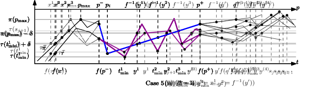
Figure 8: Examples of Case 5(i)-(iv). The broken part of the matching $f$ is indicated by fat lines.

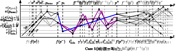
Figure 9: Examples of Case 5(v)-(vi). The broken part of the matching $f$ is indicated by fat lines.

We have now handled Case 5(i)-(iv). Examples of these cases are shown in Figure 8. We now move on to prove correctness of the remaining cases Case 5(v) and Case 5(vi).

Proof of Case 5(v).

Observe that in this case $q^{\prime\prime}=q=g(\pi(p_{\max}))$, as in Case 3. Therefore, $y^{\prime}$ and $z$ are the same as in Case 3 and must exist. We argue that $x^{\prime}$ must also exist. Indeed, we can derive $\pi(x^{(\overline{a})})\leq\tau(s_{j+1})-\delta\leq\pi(p_{\max})$, as follows. Recall that by our case distinction $f(p^{-})\leq s_{j+1}\leq f(p^{+})$. By Property 2, it follows that

$$\tau(s_{j+1})=\max(\tau[f(p^{-}),f(p^{+})])\leq\max(\pi[p^{-},p^{+}])+\delta\leq\pi(p_{\max})+\delta.$$

Now we need to prove the validity of the matching scheme. The first line follows from Claim 3.15. For the second line we need to prove that

$$\left\{{\tau(t)~{}|~{}t\in[y^{(\overline{a})},y^{\prime}]}\right\}\subseteq[\tau(s_{j+1})-2\delta,\tau(s_{j+1})]=[\pi(x^{\prime})]_{\delta}.$$

The upper bound follows from Property 1(iii). As for the lower bound, by the definition of the stopping parameter,

$$\min(\tau[y^{(\overline{a})},s_{j+1}])=\tau(y^{(\overline{a})})=\pi(p_{\max})-\delta\geq\tau(s_{j+1})-2\delta,$$

(as we just proved above). By Claim 3.9,

$$\min(\tau[s_{j+1},f(p^{+})])\geq\tau(s_{j+1})-2\delta.$$

By our case distinction and by Property 2,

$$\min(\tau[f(p^{+}),f(q^{\prime\prime})])\geq\min(\pi[p^{+},q^{\prime\prime}])-\delta\geq\tau(s_{j+1})-2\delta.$$

The validity of the third matching is implied by Claim 3.15. For the last two matchings we can apply the respective part of the proof of Case 3 verbatim. ∎

Proof of Case 5(vi).

The validity of the first matching follows from Claim 3.15 and since $x^{(\overline{a})}\geq x$. By our case distinction,

$$\left\{{\pi(p)~{}|~{}p\in[p^{+},q^{\prime\prime}]}\right\}\subseteq[\tau(s_{j+1})-\delta,\pi(p_{\max})]\subseteq[\tau(y^{(\overline{a})}]_{\delta}).$$

Thus, also the second matching is valid. For the last matching we need to prove that

$$\left\{{\tau(t)~{}|~{}t\in[y^{(\overline{a})},f(q^{\prime\prime})]}\right\}\subseteq[\tau(s_{j+1})-2\delta,\tau(s_{j+1})]=[\pi(q^{\prime\prime})]_{\delta}.$$

Again, as in Case 5(v), it holds that

$$\left\{{\tau(t)~{}|~{}t\in[y^{(\overline{a})},f(p^{+})]}\right\}\subseteq[\tau(s_{j+1})-2\delta,\tau(s_{j+1})].$$

By our case distinction and by Property 2

$$\min(\tau[f(p^{+}),f(q^{\prime\prime})])\geq\min(\pi[p^{+},q^{\prime\prime}])-\delta\geq\tau(s_{j+1})-2\delta$$

This also implies that $f(q^{\prime\prime})<s_{j+2}$, by Property 1(i). Thus, by Property 1(iii), we conclude

$$\max(\tau[f(p^{+}),f(q^{\prime\prime})])\leq\tau(s_{j+1}).$$

Together this implies the validity of the last matching. ∎

We now proved correctness of the last two cases Case 5(v) and Case 5(vi). Examples of these cases are shown in Figure 9.

It remains to prove the boundary cases, which we have ruled out so far by Assumption 3. There are three boundary cases:

1. $s_{j}=0$ and $s_{j+1}=1$,

2. $s_{j}=0$ and $s_{j+1}<1$,

3. $s_{j}>0$ and $s_{j+1}=1$.

To prove the claim in each of these cases, we can use the above proof verbatim with minor modifications. Note that in the proof, we used $s_{j}$ in its function as the minimum on the signature edge $\overline{s_{j}s_{j+1}}$, resp., we used $s_{j+1}$ in its function as the maximum on this edge. Thus, let

$$s_{\min}=\operatorname*{arg\,min}_{s\in[s_{j},s_{j+1}]}\tau(s),~{}~{}~{}s_{\max}=\operatorname*{arg\,max}_{s\in[s_{j},s_{j+1}]}\tau(s).$$

Claim 3.22.

In each of the cases (B1), (B2) and (B3), it holds that $f(p_{i})\in[s_{\min},s_{\max}]$ and $\tau(s_{\max})-\tau(s_{\min})\geq 4\delta$.

Proof.

By the theorem statement and by Definition 3.3, it holds that

$$\pi(p_{i})\notin[v_{1}]_{4\delta}\cup[v_{\ell}]_{4\delta}=[\tau(0)]_{4\delta}\cup[\tau(1)]_{4\delta}$$

i.e., the removed vertex $\pi(p_{i})$ lies very far from the endpoints of the curve $\tau$. At the same time, by Definition 3.3, in case $s_{j}=0$,

$$\tau(0)\geq\tau(s_{\min})\geq\tau(0)-\delta$$

and, in case $s_{j+1}=1$,

$$\tau(1)\leq\tau(s_{\max})\leq\tau(1)+\delta.$$

By the direction-preserving property of Definition 3.3 and by Property 2, this implies that $f(p_{i})\in[s_{\min},s_{\max}]$. In the cases where $s_{j}=0$, this implies

$$\tau(f(p_{i}))\geq\tau(s_{\min})\geq\tau(0)-\delta,$$

therefore, by the above, $\tau(f(p_{i}))\geq\tau(0)+4\delta\geq\tau(s_{\min})+4\delta$. Similarly in the cases, where $s_{j+1}=1$, we can derive that $\tau(f(p_{i}))\leq\tau(1)-4\delta\leq\tau(s_{\max})-4\delta$. In each of the cases (B1), (B2) and (B3), this implies the second part of the claim. ∎

We replace Property 1 with the following property.

Property 3 (Signature (boundary case)).

1. $\tau(s_{\max})-\tau(s_{\min})>2\delta$,

2. $\tau(s_{\min})=\min(\tau[s_{j-1},s_{j+1}])$ (if $s_{j}=0$, then $\tau(s_{\min})=\min(\tau[0,s_{j+1}])$),

3. $\tau(s_{\max})=\max(\tau[s_{j},s_{j+2}])$ (if $s_{j+1}=1$, then $\tau(s_{\max})=\max(\tau[s_{j},1])$),

4. $\tau(t)\geq\tau(t^{\prime})-2\delta$ for $s_{\min}\leq t^{\prime}<t\leq s_{\max}$,

5. if $s_{j}=0$, then $\tau(s_{\max})-\tau(s_{j+2})>2\delta$.

Property 3(ii), (iii), (iv), and (v) hold by Definition 3.3. Property 3(i) follows from Claim 3.22.

Instead of Claim 3.9 we use the claim

Claim 3.23.

If $s_{\max}\in[f(p^{-}),f(p^{+})]$ then $\left\{{\tau(t)~{}|~{}t\in[s_{\max},f(p^{+})]}\right\}\subseteq[\tau(s_{\max})-2\delta,\tau(s_{\max})]$.

Instead of Claim 3.10 we use the claim

Claim 3.24.

$s_{\min}\notin[f(p^{-}),f(p^{+})]$.

Now, the theorem follows in the boundary cases (B1), (B2) and (B3), by replacing $s_{j}$ with $s_{\min}$ and replacing $s_{j+1}$ with $s_{\max}$.

This closes the proof of Lemma 3.8 ∎

4 $(k,\ell)$-center

Data: curves $P=\{{\tau}_{1},\dots,{\tau}_{n}\}\subset\Delta_{m}$, parameters $\alpha,\beta>0$, $k,\ell\in{\rm I\!N}$

Result: candidate set $\Gamma^{k,\ell}_{\alpha,\beta}(S)\subseteq\Delta_{\ell}$

1 For each ${\tau}_{i}$, let $\mathcal{V}_{i}$ be the vertex set of its $\alpha$-signature computed by Algorithm 4;

2 Compute the union $U$ of the intervals $r=\left[w-4\alpha,w+4\alpha\right]$ for $w\in\mathcal{V}=\bigcup_{i=1}^{n}\mathcal{V}_{i}$;

3 if  $\mu(U)>24\alpha k\ell$ then

4      Return the empty set;

5else

6      Discretize $U$ with resolution $\beta$, thereby generating a set of vertices $\widehat{\mathcal{V}}$;

7       Return all possible curves consisting of $\ell$ vertices from $\widehat{\mathcal{V}}$;

Algorithm 1 Generate candidates for $(k,\ell)$-center from signature vertices

Lemma 4.1.

Given a set of curves $P=\{{\tau}_{1},\dots,{\tau}_{n}\}$ and parameters $\alpha,\beta>0$, and $k,\ell\in{\rm I\!N}$, then Algorithm 1 generates a set of candidate solutions $\Gamma^{k,\ell}_{\alpha,\beta}(S)\subseteq\Delta_{\ell}$ of size at most $\left(\left\lfloor{\frac{24\alpha k\ell}{\beta}}\right\rfloor+6k\ell\right)^{\ell}$. Furthermore, if $\alpha\geq\operatorname{opt}^{(\infty)}_{k,\ell}(P)$, then the generated set contains $k$ candidates $\tilde{C}=\tilde{c_{1}},\dots,\tilde{c_{k}}$ with

$$\operatorname{cost}_{\infty}(P,\tilde{C})\leq\alpha+\beta.$$

Proof.

Let $C=c_{1},\dots,c_{k}$ denote an optimal solution for $P$ and let $c_{i}=z_{i1},\dots,z_{i{\ell}}$ denote the vertices for each cluster center. Consider the union of intervals

$$R=\bigcup_{i=1}^{k}\bigcup_{j=1}^{\ell}[z_{ij}-4\alpha,z_{ij}+4\alpha].$$

Lemma 3.5 implies that $R$ contains all elements of $\mathcal{V}$, the signature vertices computed by Algorithm 1. Now consider the dual statement, namely, whether the vertices $z_{ij}$ are contained in the set $U$ computed by the algorithm. If there exists a $z_{ij}$ which is not contained in $U$, then Theorem 3.7 implies that we can omit $z_{ij}$ from the solution while not increasing the cost beyond $\alpha$. Therefore, let $\widehat{C}$ denote the solution where all vertices that lie outside $U$ have been omitted. Clearly, $U$ contains all remaining vertices of cluster centers in $\widehat{C}$. Therefore, $\Gamma^{k,\ell}_{\alpha,\beta}$ must contain $k$ candidates $\tilde{C}=\tilde{c_{1}},\dots,\tilde{c_{k}}$ with

$$\operatorname{cost}_{\infty}(P,\tilde{C})\leq\alpha+\beta.$$

Note that $R$ consists of at most $k\ell$ intervals and has measure at most $\mu(R)=8\alpha k\ell$. Therefore, the measure of $U$ can be at most $\mu(U)\leq\mu(R)+(2k\ell)8\alpha=24\alpha k\ell.$ In the worst case a signature vertex lies at each boundary point of $R$. Furthermore, $U$ consists of at most $\left\lceil{\frac{\mu(U)}{8\alpha}}\right\rceil\leq 3k\ell$ intervals, since each interval has measure at least $8\alpha$. ∎

Theorem 4.2.

Let ${\varepsilon}>0$ and $k,\ell\in{\rm I\!N}$ be given constants. Given a set of curves $P=\{{\tau}_{1},\dots,{\tau}_{n}\}$ we can compute a $(1+{\varepsilon})$-approximation to $\operatorname{opt}^{(\infty)}_{k,\ell}(P)$ in time $O\!\left({nm\log m}\right)$.

Proof.

We use Algorithm 3 described in Section 6 to compute a constant-factor approximation. We obtain an interval $[\delta_{\min},\delta_{\max}]$ which contains $\operatorname{opt}^{(\infty)}_{k,\ell}(P)$ and such that $\delta_{\max}/\delta_{\min}\leq 8$ by Theorem 6.2. We can now do a binary search in this interval. In each step of the binary search, we apply Algorithm 1 to $P$ a constant number of times and evaluate every candidate solution. More specifically, if we apply Algorithm 1 to $P$ with parameters $\alpha$ and $\beta={\varepsilon}\alpha$, by Lemma 4.1 we gain the following knowledge:

1. Either $\alpha<(1+{\varepsilon})\operatorname{opt}^{(\infty)}_{k,\ell}(P)$, or

2. $\alpha\geq\operatorname{opt}^{(\infty)}_{k,\ell}(P)$ and we have computed a solution with cost at most $(1+{\varepsilon})\alpha$.

In both cases, the outcome is correct. Since we want to take an exact decision during the binary search, we simply call the procedure twice with parameters $\alpha_{1}=\frac{\alpha}{1+{\varepsilon}/2},\beta_{1}=\frac{{\varepsilon}}{2}\alpha_{1}$ and $\alpha_{2}=\alpha,\beta_{2}={\varepsilon}\alpha_{2}$. Now there are three possible outcomes:

1. Either $\operatorname{opt}^{(\infty)}_{k,\ell}(P)<\alpha$, or

2. $\operatorname{opt}^{(\infty)}_{k,\ell}(P)>(1+{\varepsilon})\alpha$, or

3. $\operatorname{opt}^{(\infty)}_{k,\ell}(P)\in[\alpha,(1+{\varepsilon})\alpha]$.

So either we can take an exact decision and proceed with the binary search, or we obtain a $(1+{\varepsilon})$-approximation to the solution and we stop the search.

By Lemma 4.1 we know that the size of the candidate set $\Gamma^{k,\ell}_{\alpha,\beta}$ is $O(1)$ (where the constant depends on ${\varepsilon},k$ and $\ell$.

One execution of Algorithm 1 takes $O(nm)$ time for computing the $n$ signatures (using Algorithm 4) and $O(1)$ time for generating the candidate set. Evaluating one candidate solution (consisting of $k$ centers from the candidate set) takes $kn$ Fréchet distance computations, where one Fréchet distance computation takes time $O(m\log m)$ using the algorithm by Alt and Godau [7]. The number of binary search steps depends only on the constant ${\varepsilon}$ and so is $O(1)$, which implies the running time. ∎

5 $(k,\ell)$-median

In this section we will make use of a result by Ackermann et al. [2] for computing an approximation to the $k$-median problem under an arbitrary dissimilarity measure $D:\Delta\times\Delta\rightarrow\mathbb{R}_{0}^{+}$ on a ground set of items $\Delta$, i.e. a function that satisfies $D(x,y)=0$, iff $x\not=y$. The result roughly says that we can obtain an efficient $(1+\varepsilon)$-approximation algorithm for the $k$-median problem on input $P\subseteq\Delta$, if there is an algorithm that given a random sample of constant size returns a set of candidates for the $1$-median that contains with constant probability (over the choice of the sample) a $(1+\varepsilon)$-approximation to the $1$-median.

We restate the sampling property defined by Ackermann et al. ([2],Property 4.1).

Definition 5.1 (sampling property).

We say a dissimilarity measure D satisfies the (weak) $[{\varepsilon},\lambda]$-sampling property iff there exist integer constants $m_{{\varepsilon},\lambda}$ and $t_{{\varepsilon},\lambda}$ such that for each $P\subseteq\Delta$ of size $n$ and for each uniform sample multiset $S\subseteq P$ of size $m_{{\varepsilon},\lambda}$ a set $\Gamma(S)\subseteq\Delta$ of size at most $t_{{\varepsilon},\lambda}$ can be computed satisfying

$$\Pr\left[\exists\tilde{c}\in\Gamma(S):D(P,\tilde{c})\leq(1+{\varepsilon})\operatorname{opt}(P)\right]\geq 1-\lambda.$$

Furthermore, $\Gamma(S)$ can be computed in time depending on $\gamma,\delta$ and $m_{{\varepsilon},\lambda}$ only.

It is likely that the sampling property (Definition 5.1) does not hold for the Fréchet distance for arbitrary value of $\ell$. We will therefore prove a modified sampling property, which allows the size of the sample to depend on $\ell$.

The following lemma intuitively says that curves that lie far away from a candidate median have little influence on the shape of the candidate median.

Lemma 5.2.

Given a set of $n$ curves $P=\{\tau_{1},\ldots,\tau_{n}\}$ and a polygonal curve $\pi$, it holds that

$$\operatorname{cost}_{1}(P,\widehat{\pi})\leq(1+{\varepsilon})\operatorname{cost}_{1}(P,\pi)$$

for a curve $\widehat{\pi}$ obtained from $\pi$ by omitting any subset of vertices lying outside the following union $R_{S}$:

$$R_{S}=\bigcup_{1\leq i\leq n\atop x_{i}\leq\frac{2x_{1}}{{\varepsilon}}}\;\bigcup_{v\in\mathcal{V}(\sigma_{i})}[v-4x_{i},v+4x_{i}],$$

where the $\tau_{i}$ are sorted in increasing order of $x_{i}=d_{F}\!\left({{\tau}_{i},\pi}\right)$ and where $\sigma_{i}$ is the $x_{i}$-signature of ${\tau}_{i}\in P$.

Proof.

By Lemma 3.5, the curve $\pi$ has a vertex in each range centered at the vertices of $\sigma_{i}$. These will not be omitted, therefore it is ensured that $\widehat{\pi}$ has at least 2 vertices, i.e. defines a curve. By Theorem 3.7, it holds that $d_{F}\!\left({\widehat{\pi},{\tau}_{i}}\right)\leq x_{i}$ for the curves ${\tau}_{i}$ with $x_{i}\leq\frac{2x_{1}}{{\varepsilon}}$, that is, for the curves that lie close to $\pi$. We now argue using the triangle inequality that the distances to the curves that lie further away are only altered by a factor of at most $(1+{\varepsilon})$. Consider any index $i$, such that $x_{i}>\frac{2x_{1}}{{\varepsilon}}=\widehat{x}$. By the triangle inequality, it holds that

$$d_{F}\!\left({\widehat{\pi},{\tau}_{i}}\right) \leq d_{F}\!\left({\widehat{\pi},{\tau}_{1}}\right)+d_{F}\!\left({{\tau}_{1},{\tau}_{i}}\right)$$

$$\leq d_{F}\!\left({\widehat{\pi},{\tau}_{1}}\right)+d_{F}\!\left({{\tau}_{1},\pi}\right)+d_{F}\!\left({\pi,{\tau}_{i}}\right)$$

$$\leq x_{1}+x_{1}+x_{i}$$

$$< (1+{\varepsilon})x_{i}$$

Therefore,

$$\operatorname{cost}_{1}(P,\widehat{\pi})\leq\sum_{x_{i}\leq\widehat{x}}d_{F}\!\left({\pi,{\tau}_{i}}\right)+\sum_{x_{i}>\widehat{x}}(1+{\varepsilon})d_{F}\!\left({\pi,{\tau}_{i}}\right)\leq(1+{\varepsilon})\operatorname{cost}_{1}(P,\pi).$$

∎

The following lemma is in similar spirit as Lemma 5.2. We prove that the basic shape of a candidate median can be approximated based on a constant-size sample.

Lemma 5.3.

There exist integer constant $m_{{\varepsilon},\lambda,\ell}$ such that given a set of curves $P$ and a curve $\pi=u_{1},\dots,u_{\ell}$ for each uniform sample multiset $S\subseteq P$ of size $m_{{\varepsilon},\lambda,\ell}\geq\left\lceil{\frac{8\ell}{{\varepsilon}}\left(\log\left(\frac{1}{\lambda}\right)+\log(\ell)\right)}\right\rceil$ it holds that

$$\Pr\left[\operatorname{cost}_{1}(P,\widehat{\pi})\leq(1+{\varepsilon})\operatorname{cost}_{1}(P,\pi)\right]\geq 1-\lambda,$$

for a curve $\widehat{\pi}$ obtained from $\pi$ by omitting any subset of vertices lying outside the following union $R_{S}$:

$$R_{S}=\bigcup_{{\tau}_{i}\in S}\;\bigcup_{v\in\mathcal{V}(\sigma_{i})}[v-4x_{i},v+4x_{i}],$$

where the $\tau_{i}$ are sorted in increasing order of $x_{i}=d_{F}\!\left({{\tau}_{i},\pi}\right)$ and where $\sigma_{i}$ is the $x_{i}$-signature of ${\tau}_{i}\in S$.

Proof.

If all vertices of $\pi$ are contained in $R_{S}$, then $\pi=\widehat{\pi}$ and the claim is implied. However, this is not necessarily the case. In the following, we consider a fixed vertex $u_{j}$ and we prove that it is either contained in $R_{S}$ with sufficiently high probability or ignoring it will not increase the cost of a solution significantly.

For this purpose, let $T_{j}\subseteq P$ be the subset of curves ${\tau}_{i}$ with

$$u_{j}\in\bigcup_{v\in\mathcal{V}(\sigma_{i})}[v-4x_{i},v+4x_{i}].$$

If any curve of $T_{j}$ is contained in our sample $S$, then $u_{j}$ is contained in $R_{S}$.

We distinguish two cases. If $T_{j}$ is large enough then $u_{j}$ is contained in $R_{S}$ with high probability, or we argue that the total change in cost resulting from omitting $u_{j}$ from $\pi$ will be small. We will first argue that for all $j$ with $1\leq j\leq\ell$ and with $T_{j}>\frac{{\varepsilon}n}{4\ell}$ we obtain for our choice of $m_{{\varepsilon},\lambda,\ell}$ that at least one element of $T_{j}$ is contained in $S$. Indeed, we have

$$\Pr[T_{j}\cap S=\emptyset] \leq(1-|T_{j}|/n)^{m_{{\varepsilon},\lambda,\ell}}\leq\left(1-\frac{{\varepsilon}}{4\ell}\right)^{m_{{\varepsilon},\lambda,\ell}}.$$ (4)

We use the union bound, to estimate the probability that this event fails for at least one of the sets $T_{j}$ in question. We choose the parameter $m_{{\varepsilon},\lambda,\ell}$ large enough, such that it holds for the failure probability that

$$\lambda\leq\ell\left(1-\frac{{\varepsilon}}{4\ell}\right)^{m_{{\varepsilon},\lambda,\ell}}.$$

For this, it suffices to choose

$$m_{{\varepsilon},\lambda,\ell} \geq\left\lceil{\frac{8\ell}{{\varepsilon}}\left(\log\left(\frac{1}{\lambda}\right)+\log(\ell)\right)}\right\rceil$$

to obtain that with probability at least $1-\lambda$ for all $1\leq j\leq\ell$, simultaneously, we have that at least one element of $T_{j}$ is in $S$, if $|T_{j}|\geq\frac{{\varepsilon}n}{4\ell}$.

Now consider the set of curves $T=\{T_{j}:1\leq j\leq\ell,T_{j}\cap S=\emptyset\}$. By our previous considerations we have that with probability at least $1-\lambda$, $T\subseteq\left\{T_{j}\left|1\leq j\leq\ell,|T_{j}|\leq\frac{{\varepsilon}n}{4\ell}\right.\right\}$. We will assume in the following that this event happens.

Let $\tilde{\pi}$ denote the curve obtained from $\pi$ by removing all vertices from $R_{S}$, which is equivalent to removing all vertices $u_{j}$ with $T_{j}\in T$.

In the following, let $P_{T}=\bigcup_{T^{\prime}\in T}T^{\prime}$ be the set of input curves that are contained in one of the sets in $T$. By Theorem 3.7, it holds for any curve ${\tau}_{i}\in P\setminus P_{T}$, that $d_{F}\!\left({\tilde{\pi},{\tau}_{i}}\right)\leq d_{F}\!\left({\pi,{\tau}_{i}}\right)=x_{i}$, i.e., their distances do not increase beyond $x_{i}$ by the removal. Let ${\tau}_{q}$ be the curve of this set with minimal distance to $\pi$ (i.e. with smallest index $q$). Since at least half of the input curves have to lie within a radius of $\frac{2}{n}\operatorname{cost}_{1}(P,\pi)$ from $\pi$ (two times the average distance of the input curves to $\pi$) and since the union of the sets from $T$ has size less than $n/2$ (with probability at least $1-\lambda$), this implies that $x_{q}\leq\frac{2}{n}\operatorname{cost}_{1}(P,\pi)$. Therefore,

$$\operatorname{cost}_{1}(P,\tilde{\pi}) =\operatorname{cost}_{1}(P\setminus P_{T},\tilde{\pi})+\operatorname{cost}_{1}(P_{T},\tilde{\pi})$$

$$\leq\operatorname{cost}_{1}(P\setminus P_{T},\pi)+\sum_{{\tau}\in P_{T}}\left(d_{F}\!\left({{\tau},\pi}\right)+d_{F}\!\left({\pi,{\tau}_{q}}\right)+d_{F}\!\left({{\tau}_{q},\tilde{\pi}}\right)\right)$$

$$\leq\operatorname{cost}_{1}(P\setminus P_{T},\pi)+\operatorname{cost}_{1}(P_{T},\pi)+2|P_{T}|x_{q}$$

$$\leq\operatorname{cost}_{1}(P,\pi)+\frac{{\varepsilon}n}{4}\cdot\frac{4\operatorname{cost}_{1}(P,\pi)}{n}$$

$$=\left(1+{{\varepsilon}}\right)\operatorname{cost}_{1}(P,\pi).$$

∎

5.1 Generating Candidate Solutions

Our next step is to define an algorithm that generates a set of candidate curves from the sample set.

Data: curves $S=\{{\tau}_{1},\dots,{\tau}_{s}\}\subset\Delta_{m}$, parameters $\alpha,\beta>0$, $\ell\in{\rm I\!N}$

Result: candidate set $\Gamma^{\ell}_{\alpha,\beta}(S)\subseteq\Delta_{\ell}$

1 For each ${\tau}_{i}$, let $\mathcal{V}_{i}$ be the vertex set of the signature of size at most $\ell+3$ (Theorem 7.6);

2 Compute the union $U$ of the intervals $r=\left[v-8\alpha,v+8\alpha\right]$ for $v\in\mathcal{V}=\bigcup_{i=1}^{s}\mathcal{V}_{i}$;

3 Discretize $U$ with resolution $\beta$, thereby generating a set of vertices $\widehat{\mathcal{V}}$;

4 Return all possible curves consisting of $\ell$ vertices from $\widehat{\mathcal{V}}$;

Algorithm 2 Generate candidates for $(1,\ell)$-median from signature vertices

We prove some properties of Algorithm 2 and of the candidate set generated by it. This proof serves as a basis for the proof of the sampling property in Theorem 5.7.

Lemma 5.4.

Given a set of curves $S=\{{\tau}_{1},\dots,{\tau}_{s}\}$ and parameters $\alpha,\beta,{\varepsilon}>0$, and $\ell\in{\rm I\!N}$, with $\alpha\geq\min_{1\leq i\leq s}\frac{d_{F}\!\left({{\tau}_{i},c_{s}}\right)}{{\varepsilon}}$, where $c_{s}$ denotes an optimal $(1,\ell)$-median of $S$. There exist $\widehat{c}\in\Delta_{\ell}$ with

$$\operatorname{cost}_{1}(S,\widehat{c})\leq(1+{\varepsilon})\operatorname{opt}^{(1)}_{1,\ell}(S),$$

and Algorithm 2 computes a set of candidates $\Gamma^{\ell}_{\alpha,\beta}(S)\subseteq\Delta_{\ell}$ of size $\left({\frac{16\alpha s(\ell+3)}{\beta}}\right)^{\ell}$ which contains an element $\tilde{c}$, such that

$$d_{F}\!\left({\widehat{c},\tilde{c}}\right)\leq\beta.$$

Proof.

Let ${\tau}_{1},\dots,{\tau}_{s}$ denote the input curves in the increasing order of their distance denoted by $x_{i}=d_{F}\!\left({{c}_{s},{\tau}_{i}}\right)$. For every ${\tau}_{i}$, consider its $x_{i}$-signature denoted by $\sigma_{i}$. By Lemma 3.5, each vertex of ${c}_{s}$ lies within distance $4x_{i}$ to a vertex of some signature $\sigma_{i}$ otherwise we can omit it by Theorem 3.7. Hence, there must be a solution where ${c}_{s}$ has its vertices in the union of the intervals.

$$\bigcup_{i=1}^{s}\bigcup_{v\in\mathcal{V}(\sigma_{i})}[v-4x_{i},v+4x_{i}].$$

Since $x_{i}$ could be very large, we cannot cover this entire region with candidates. Instead, we consider the following union of intervals:

$$R_{S}=\bigcup_{x_{i}\leq\widehat{x}}\;\bigcup_{v\in\mathcal{V}(\sigma_{i})}[v-4x_{i},v+4x_{i}],$$

with $\widehat{x}=\frac{2x_{1}}{{\varepsilon}}$. Now, let $\widehat{{c}}$ be the median obtained from ${c}_{s}$ by omitting all vertices which do not lie in $R_{S}$. Lemma 5.2 implies $\operatorname{cost}_{1}(S,\widehat{{c}})\leq(1+{\varepsilon})\operatorname{cost}_{1}(S,{c}_{s}).$

Clearly, the generated set contains a curve $\tilde{{c}}$ which lies within Fréchet distance $\beta$ of $\widehat{{c}}$. Indeed, by Lemma 7.1, the vertices of $\sigma_{i}$ are contained in the set of signature vertices computed by Algorithm 2, since Corollary 3.6 implies that $\ell\geq|\mathcal{V}\!\left({{c}_{s}}\right)|\geq|\mathcal{V}\!\left({\sigma_{i}}\right)|-2$. If a signature of size $\ell+3$ does not exists, then by the general position assumption, there must be a signature of size $\ell+2$. The algorithm sets $\widehat{x}=2\alpha\geq 2x_{1}/{\varepsilon}$. Therefore, the generated candidate set covers the region $R_{S}$ with resolution $\beta$. ∎

Before we prove the modified sampling property we prove the following two easy lemmas.

Lemma 5.5.

Let $\lambda>0$. Given a set of curves $P$, for each uniform sample multiset $S\subseteq P$ it holds that

$$\Pr\left[\operatorname{cost}_{1}(S,c)\geq\frac{|S|}{\lambda n}\operatorname{opt}^{(1)}_{1,\ell}(P)\right]\leq\lambda,$$

where $c$ is an optimal median of $P$.

Proof.

It holds that

$$\operatorname{E}\left[{\operatorname{cost}_{1}(S,c)}\right]=\frac{|S|}{n}\operatorname{opt}^{(1)}_{1,\ell}(P).$$

Since $\operatorname{cost}_{1}(S,c)$ is a nonnegative random variable we can apply Markov’s inequality and obtain

$$\Pr\left[\operatorname{cost}_{1}(S,c)\geq\frac{\operatorname{E}\left[{\operatorname{cost}_{1}(S,c)}\right]}{\lambda}\right]\leq\lambda,$$

which implies the claim. ∎

Lemma 5.6.

Let $\lambda>0$. Given a set of curves $P$, for each uniform sample multiset $S\subseteq P$ of size at least $\left\lceil{5\log(\frac{1}{\lambda})}\right\rceil+1$ it holds that

$$\Pr\left[{12\operatorname{opt}_{1,\ell}^{(1)}(S)\geq\min_{\tau\in P}d_{F}\!\left({\tau,c}\right)}\right]\geq 1-\lambda,$$

where $c$ denotes an optimal $(1,\ell)$-median of $P$.

Proof.

We analyze two cases. For the first case, assume that there exists a curve $q\in\Delta_{\ell}$, such that

$$\left\lvert\left\{{\tau\in P:d_{F}\!\left({q,\tau}\right)\leq r}\right\}\right\rvert\geq\frac{5}{7}|P|,$$

where $r=\frac{d_{F}\!\left({q,c}\right)}{5}$. That is, a large fraction of $P$ lies within a small ball far away from the optimal center. We let

$$Q=\left\{{\tau\in P:d_{F}\!\left({q,\tau}\right)<2r}\right\},$$

and we claim that $Q$ has size at most $\frac{6}{7}|P|$. Assume the opposite for the sake of contradiction. In this case, it follows by the triangle inequality that

$$\operatorname{cost}_{1}(P,q) \leq\operatorname{cost}_{1}(P,c)-|Q|r+|P\setminus Q|5r\leq\operatorname{cost}_{1}(P,c)-\frac{1}{7}|P|r<\operatorname{cost}_{1}(P,c).$$

This would imply that $c$ is not optimal. We analyze the event that at least one curve of $P$ lies within Fréchet distance $r$ of $q$ and at least one curve lies further than $2r$ from $q$. If this event happens, then again by the triangle inequality

$$\operatorname{opt}^{(1)}_{1,\ell}(S)\geq\max_{\pi,\pi^{\prime}\in S}d_{F}\!\left({\pi,\pi^{\prime}}\right)\geq r\geq\frac{\min_{\tau\in P}d_{F}\!\left({c,\tau}\right)}{6}.$$

Clearly, it holds for the $i$th sample point $s_{i}$, that

$$\Pr\left[{d_{F}\!\left({s_{i},q}\right)\leq r}\right]\geq\frac{5}{7}~{}~{}\text{and}~{}~{}\Pr\left[{d_{F}\!\left({s_{i},q}\right)\geq 2r}\right]\geq\frac{1}{7}.$$

Using this, we can show that $\left\lceil{5\log(\frac{1}{\lambda})}\right\rceil$ samples suffice to ensure that this event happens with probability of at least $(1-\lambda)$.

Now, assume the second case that no such $q$ exists. Let $s_{1}$ be the first sample point and let $\widehat{s_{1}}$ be its minimum-error $\ell$-simplification (Definition 3.1). We need to prove the claim in the case that

$$12d_{F}\!\left({s_{1},\widehat{s_{1}}}\right)<d_{F}\!\left({s_{1},c}\right),$$ (5)

since $\operatorname{opt}^{(1)}_{1,\ell}(S)$ is lower-bounded by $d_{F}\!\left({s_{1},\widehat{s_{1}}}\right)$. By the case analysis, it holds that

$$\left\lvert\left\{{\tau\in P:d_{F}\!\left({\widehat{s_{1}},\tau}\right)\leq r}\right\}\right\rvert<\frac{5}{7}|P|,$$

for $r=\frac{d_{F}\!\left({\widehat{s_{1}},c}\right)}{5}$. Therefore, it holds for each of the remaining sample points $s_{i}$, for $1<i\leq|S|$, that

$$\Pr\left[{d_{F}\!\left({\widehat{s_{1}},s_{i}}\right)>r}\right]\geq\frac{2}{7}.$$

In case this event happens, it holds by the triangle inequality

$$d_{F}\!\left({s_{1},s_{i}}\right)\geq d_{F}\!\left({s_{i},\widehat{s_{1}}}\right)-d_{F}\!\left({\widehat{s_{1}},s_{1}}\right)\geq r-d_{F}\!\left({\widehat{s_{1}},s_{1}}\right)\geq\frac{d_{F}\!\left({c,s_{1}}\right)-d_{F}\!\left({s_{1},\widehat{s_{1}}}\right)}{5}-d_{F}\!\left({\widehat{s_{1}},s_{1}}\right)\geq\frac{d_{F}\!\left({c,s_{1}}\right)}{10}.$$

The analysis of this event is almost the same as in the first case. In this case, a total number of $\left\lceil{5\log(\frac{1}{\lambda})}\right\rceil+1$ samples suffices to ensure that this event happens with probability of at least $(1-\lambda)$. ∎

We are now ready to prove the modified sampling property.

Theorem 5.7.

There exist integer constants $m_{{\varepsilon},\lambda,\ell}$ and $t_{{\varepsilon},\lambda,\ell}$ such that given a set of curves $P=\left\{{{\tau}_{1},\dots,{\tau}_{n}}\right\}$ for a uniform sample multiset $S\subseteq P$ of size $m_{{\varepsilon},\lambda,\ell}$ we can generate a candidate set $\Gamma(S)\subset\Delta_{\ell}$ of size $t_{{\varepsilon},\lambda,\ell}$ satisfying

$$\Pr\left[\exists q\in\Gamma(S):\operatorname{cost}_{1}(P,q)\leq(1+{\varepsilon})\operatorname{opt}^{(1)}_{1,\ell}(P)\right]\geq 1-\lambda.$$

Furthermore, we can compute $\Gamma(S)$ in time depending on $\ell,\lambda$ and ${\varepsilon}$ only.

Proof.

Let $\lambda^{\prime}=\frac{\lambda}{4}$ and ${\varepsilon}^{\prime}=\frac{{\varepsilon}}{4}$. Let $c$ denote an optimal $(1,\ell)$-median of $P$ and let $c_{s}$ denote an optimal $(1,\ell)$-median of $S$. We use the algorithm described in Section 6 to compute a constant-factor approximation to $\operatorname{opt}^{(1)}_{1,\ell}(S)$ and obtain an interval $[\delta_{S}^{\min},\delta_{S}^{\max}]$ which contains $\operatorname{opt}^{(1)}_{1,\ell}(S)$ and by Theorem 6.3 it holds that $\delta_{S}^{\max}/\delta_{S}^{\min}\leq 65$. We apply Algorithm 2 to $S$ with parameters

$$\alpha=\frac{6\delta_{S}^{\max}}{{\varepsilon}^{\prime}}~{}~{}\text{ and }~{}~{}\beta=\frac{{\varepsilon}^{\prime}\lambda^{\prime}\delta_{S}^{min}}{|S|},$$

and obtain a set $\Gamma^{\ell}_{\alpha,\beta}$.

With the help of Lemma 5.3, we can now adapt the proof of Lemma 5.4 to our probabilistic setting. Let ${c}=z_{1},\dots,z_{\ell}$ be an optimal $(1,\ell)$-median of $P$. Let ${\tau}_{1},\dots,{\tau}_{n}$ denote the input curves in the increasing order of their distance denoted by $x_{i}=d_{F}\!\left({{c},{\tau}_{i}}\right)$. For every ${\tau}_{i}$, consider its $x_{i}$-signature denoted by $\sigma_{i}$. By Lemma 3.5, each vertex of ${c}$ lies within distance $4x_{i}$ to a vertex of some signature $\sigma_{i}$, otherwise we can omit it by Theorem 3.7. Hence, there must be a $(1,\ell)$-median whose vertex set is contained in the union of the intervals

$$\bigcup_{{\tau}_{i}\in P}\bigcup_{v\in\mathcal{V}(\sigma_{i})}[v-4x_{i},v+4x_{i}].$$

Let this solution be denoted ${c}$.

So, consider the following union of intervals:

$$R_{1}=\bigcup_{{\tau}_{i}\in S}\bigcup_{v\in\mathcal{V}(\sigma_{i})}[v-4x_{i},v+4x_{i}],$$

Let $\widehat{{c}_{1}}$ be the median obtained from ${c}$ by omitting all vertices which do not lie in $R_{1}$. Lemma 5.3 implies

$$\Pr\left[\operatorname{cost}_{1}(P,\widehat{{c}_{1}})\leq(1+{\varepsilon}^{\prime})\operatorname{cost}_{1}(P,{c})\right]\geq 1-\lambda^{\prime},$$

if we choose $|S|\geq\left\lceil{\frac{8\ell}{{\varepsilon}}\left(\log\left(\frac{1}{\lambda^{\prime}}\right)+\log(\ell)\right)}\right\rceil$.

So, now consider the following union of intervals:

$$R_{2}=\bigcup_{{\tau}_{i}\in P\atop x_{i}\leq\widehat{x}}\bigcup_{v\in\mathcal{V}(\sigma_{i})}[v-4x_{i},v+4x_{i}],$$

where $\widehat{x}=\frac{2x_{1}}{{\varepsilon}^{\prime}}$. Let $\widehat{{c}_{2}}$ be the median obtained from $\widehat{{c}_{1}}$ by omitting all vertices which do not lie in $R_{2}$. Lemma 5.6 implies that if $|S|\geq\left\lceil{5\log(\frac{1}{\lambda^{\prime}})}\right\rceil+1$, then it holds with a probability of at least $(1-\lambda^{\prime})$ that $x_{1}\leq 12\operatorname{opt}^{{(1)}}_{1,\ell}(S).$ Algorithm 2 sets $\widehat{x}=4\alpha$, therefore

$$\widehat{x}=\frac{24\delta_{S}^{\max}}{{\varepsilon}^{\prime}}\geq\frac{24\operatorname{opt}^{(1)}_{1,\ell}(S)}{{\varepsilon}^{\prime}}\geq\frac{2x_{1}}{{\varepsilon}^{\prime}}.$$

Thus, we can apply Lemma 5.2 and obtain

$$\operatorname{cost}_{1}(P,\widehat{{c}_{2}})\leq(1+{\varepsilon}^{\prime})\operatorname{cost}_{1}(P,\widehat{{c}_{1}}).$$

Therefore, with probability $1-2\lambda^{\prime}$, the generated set $\Gamma^{\ell}_{\alpha,\beta}$ contains a curve $\tilde{{c}}$ which lies within Fréchet distance $\beta$ of $\widehat{{c}_{2}}$.

Lemma 5.5 implies that with probability at least $1-\lambda^{\prime}$ it holds that

$$\operatorname{opt}^{(1)}_{1,\ell}(S)\leq\operatorname{cost}_{1}(S,c)\leq\frac{|S|}{\lambda^{\prime}n}\operatorname{opt}^{(1)}_{1,\ell}(P).$$

Thus, with the same probability it holds that

$$\beta=\frac{{\varepsilon}^{\prime}\lambda^{\prime}\delta_{S}^{min}}{|S|}\leq\frac{{\varepsilon}^{\prime}\lambda^{\prime}\operatorname{opt}^{(1)}_{1,\ell}(S)}{|S|}\leq\frac{{\varepsilon}^{\prime}\operatorname{opt}^{(1)}_{1,\ell}(P)}{n}.$$

We conclude that with probability $1-3\lambda^{\prime}>1-\lambda$ (union bound) there exists a candidate in $\tilde{c}\in\Gamma^{\ell}_{\alpha,\beta}$ such that

$$\operatorname{cost}_{1}(P,\tilde{c}) \leq\operatorname{cost}_{1}(P,\widehat{c_{2}})+\beta n\leq(1+{\varepsilon}^{\prime})\operatorname{cost}_{1}(P,\widehat{c_{1}})+\beta n$$

$$\leq(1+{\varepsilon}^{\prime})^{2}\operatorname{cost}_{1}(P,c)+\beta n\leq((1+{\varepsilon}^{\prime})^{2}+{\varepsilon}^{\prime})\operatorname{opt}^{(1)}_{1,\ell}(P)\leq(1+{\varepsilon})\operatorname{opt}^{(1)}_{1,\ell}(P).$$

Furthermore, by Lemma 5.4 the size of $\Gamma^{\ell}_{\alpha,\beta}$ is bounded as follows

$$t_{{\varepsilon}^{\prime},\lambda^{\prime},\ell}\leq\left({\frac{16\alpha|S|(\ell+3)}{\beta}}\right)^{\ell}=\!\left({c_{1}{\varepsilon}^{-4}\lambda^{-1}\ell^{3}\!\left({\log^{2}\!\left({\frac{1}{\lambda}}\right)+\log^{2}\ell}\right)}\right)^{\ell},$$

where $c_{1}$ is a sufficiently large constant. ∎

The following theorem follows from Ackermann et al. [2] (Theorem 5.7). For this purpose, recall that the analysis of Ackermann et al. does not require the distance function to satisfy the triangle inequality. Therefore we can adopt the $(k,\ell)$-median formulation from Section 2.1 which uses the dissimilarity measure $D$ on the set $\Delta_{\ell}\cup P$. To achieve the running time we use Alt and Godau’s algorithm [7] for distance computations.

Theorem 5.8.

Let ${\varepsilon},k,\ell>0$ be constants. Given a set of curves $P=\left\{{{\tau}_{1},\dots,{\tau}_{n}}\right\}\subset\Delta_{m}$, there exists an algorithm that with constant probability returns a $(1+{\varepsilon})$-approximation to the $(k,\ell)$-median problem for input instance $P$, and that has running time $O(nm\log m)$.

6 Constant-factor approximation in various cases

It is not difficult to compute a constant-factor approximation for our problem. We include the details for the sake of completeness. Our algorithm first simplifies the input curves before applying a known approximate clustering algorithm designed for general metric spaces. Note that an approximation scheme which first applies clustering and then simplification does not yield the same running time, since the distance computations are expensive.

Data: curves $P=\left\{{{\tau}_{1},\dots,{\tau}_{n}}\right\}$, parameters $k>0,\ell>0$

Result: cluster centers $C=\left\{{c_{1},\dots,c_{k}}\right\}$ and cost $D$

1 For each ${\tau}_{i}$ we compute an approximate minimum-error $\ell$-simplification $\widehat{{\tau}_{i}}$ (Lemma 7.9);

2 We apply a known approximation algorithm for clustering in general metric spaces on $\widehat{P}=\widehat{{\tau}_{1}},\dots,\widehat{{\tau}_{n}}$ (i.e., Gonzales’ algorithm [35] for $k$-center and Chen’s algorithm [21] for $k$-median);

3 We return the resulting cluster centers $C={c}_{1},\dots,{c}_{k}$ with approximate cost

$$D_{\infty} = \operatorname{cost}_{\infty}(C,\widehat{P})+\max_{1\leq i\leq n}d_{F}\!\left({{\tau}_{i},\widehat{{\tau}_{i}}}\right)$$

$$D_{1} = \operatorname{cost}_{1}(C,\widehat{P})+\sum_{1\leq i\leq n}d_{F}\!\left({{\tau}_{i},\widehat{{\tau}_{i}}}\right)$$

for $(k,\ell)$-center and $(k,\ell)$-median, respectively;

Algorithm 3 Constant-factor approximation for $(k,\ell)$-clustering

Lemma 6.1.

The cost $D_{\infty}$ (resp., $D_{1}$) and solution $C$ computed by Algorithm 3 constitute a $(\alpha+\beta+\alpha\beta)$-approximation to the $(k,\ell)$-center problem (resp., the $(k,\ell)$-median problem), where $\alpha$ is the approximation factor of the simplification step and $\beta$ is the approximation factor of the clustering step.

Proof.

We first discuss the case of $(k,\ell)$-center. The $(k,\ell)$-median will follow with a simple modification. First, we have that

$$D_{\infty} = \operatorname{cost}_{\infty}(C,\widehat{P})+\max_{1\leq i\leq n}d_{F}\!\left({{\tau}_{i},\widehat{{\tau}_{i}}}\right)$$

$$= \max_{1\leq i\leq n}\;\min_{{c}\in C}d_{F}\!\left({\widehat{{\tau}_{i}},{c}}\right)+\max_{1\leq i\leq n}d_{F}\!\left({{\tau}_{i},\widehat{{\tau}_{i}}}\right)$$

$$\geq \max_{1\leq i\leq n}\;\min_{{c}\in C}\!\left({d_{F}\!\left({\widehat{{\tau}_{i}},{c}}\right)+d_{F}\!\left({{\tau}_{i},\widehat{{\tau}_{i}}}\right)}\right)$$

$$\geq \max_{1\leq i\leq n}\;\min_{{c}\in C}d_{F}\!\left({{\tau}_{i},{c}}\right)$$

$$\geq \operatorname{cost}_{\infty}(C,P).$$

Now, let $\delta^{*}$ be the optimal cost for a solution to the $(k,\ell)$-center problem for $P=\{{\tau}_{1},\dots,{\tau}_{n}\}$. It holds that

$$D_{\infty} \leq \operatorname{cost}_{\infty}(C,\widehat{P})+\alpha\delta^{*},$$

since $\delta^{*}$ is lower bounded by the distance of any input time series to its optimal $\ell$-simplification and this is the minimal Fréchet distance the time series can have to any curve with at most $\ell$ vertices. Now, consider an optimal solution $C^{*}$ with cost $\delta^{*}$. We can relate it to $D_{\infty}$ as follows. In the following, let $p_{i}\in C^{*}$ be the center of this optimal solution which is closest to ${\tau}_{i}$.

$$\delta^{*} = \max_{i=1,\ldots,n}\;d_{F}\!\left({{\tau}_{i},p_{i}}\right)$$

$$\geq \max_{i=1,\ldots,n}\;\!\left({d_{F}\!\left({\widehat{{\tau}_{i}},p_{i}}\right)-d_{F}\!\left({{\tau}_{i},\widehat{{\tau}_{i}}}\right)}\right)$$

$$\geq \max_{i=1,\ldots,n}\;d_{F}\!\left({\widehat{{\tau}_{i}},p_{i}}\right)-\max_{i=1,\ldots,n}d_{F}\!\left({{\tau}_{i},\widehat{{\tau}_{i}}}\right)$$

$$\geq \operatorname{cost}_{\infty}(C^{*},\widehat{P})-\max_{i=1,\ldots,n}d_{F}\!\left({{\tau}_{i},\widehat{{\tau}_{i}}}\right)$$

$$\geq \frac{1}{\beta}\!\left({\operatorname{cost}_{\infty}(C,\widehat{P})}\right)-\alpha\delta^{*}$$

$$\geq \frac{1}{\beta}\!\left({D_{\infty}-\alpha\delta^{*}}\right)-\alpha\delta^{*}$$

It follows that $D_{\infty}\leq(\alpha+\beta+\alpha\beta)\delta^{*}$.

∎

Theorem 6.2.

Given a set of $n$ curves $P=\{{\tau}_{1},\ldots,{\tau}_{n}\}\subseteq\Delta_{m}$ and parameters $k,\ell\in{\rm I\!N}$, we can compute an $8$-approximation to $\operatorname{opt}^{(\infty)}_{k,\ell}(P)$ and a witness solution in time $O(knm\ell\log(m\ell))$.

Proof.

The theorem follows by Lemma 6.1 and by setting $\alpha=\beta=2$. We use Lemma 7.9 to obtain a $2$-approximate simplification for each curve. Then, we use Gonzales’ algorithm which yields a $2$-approximation for the simplifications. Each distance computation takes $O(m\ell\log(m\ell))$ time using Alt and Godau’s algorithm [7]. ∎

Theorem 6.3.

Given a set of $n$ curves $P=\{{\tau}_{1},\ldots,{\tau}_{n}\}\subseteq\Delta_{m}$ and parameters $k,\ell\in{\rm I\!N}$, we can compute a $65$-approximation to $\operatorname{opt}^{(1)}_{k,\ell}(P)$ and a witness solution in time $O((nk+k^{7}\log^{5}n)m\ell\log(m\ell))$.

Proof.

The theorem follows from Lemma 6.1 and by setting $\alpha=2$ and $\beta=21$. We use Lemma 7.9 to obtain a $2$-approximate simplification for each curve. Then, we use the algorithm of Chen [21] to solve the discrete version of the $k$-median problem on the simplifications. Each distance computation takes $O(m\ell\log(m\ell))$ time using Alt and Godau’s algorithm [7]. Chen’s algorithm yields an $10.5$-approximation for the discrete problem, where the centers are constrained to lie in $P$. Since the Fréchet distance satisfies the triangle inequality, this implies a $21$-approximation for our problem. Therefore, setting $\beta=21$ yields a correct bound. ∎

These results can be easily extended to a $(k,\ell)$-means variant of the problem, as well as to multivariate time series, using known simplification algorithms, such as the algorithm by Abam et al. [1].

7 On computing signatures

In this section we discuss how to compute signatures efficiently. Our signatures have a unique hierarchical structure as testified by Lemma 7.1. Together with the concept of vertex permutations (Definition 7.2) this allows us to construct a data structure, which supports efficient queries for the signature of a given size (Theorem 7.6). If the parameter $\delta$ is given, we can compute a signature in linear time using Algorithm 4. Furthermore, we show that our signatures are approximate simplifications in Lemma 7.9.

Lemma 7.1.

Given a polygonal curve $\tau:[0,1]\rightarrow{\rm I\!R}$ with vertices in general position, there exists a series of signatures $\sigma_{1},\sigma_{2},\dots,\sigma_{k}$ and corresponding parameters $0=\delta_{1}<\delta_{2}<\dots<\delta_{k+1}$, such that

1. $\sigma_{i}$ is a $\delta$-signature of $\tau$ for any $\delta\in[\delta_{i},\delta_{i+1})$,

2. the vertex set of $\sigma_{i+1}$ is a subset of the vertex set of $\sigma_{i}$,

3. $\sigma_{k}$ is the linear interpolation of $\tau(0)$ and $\tau(1)$.

Proof.

We set $\sigma_{1}=\tau$ and obtain the desired series by a series of edge contractions. Clearly, $\sigma_{1}$ is a minimal $\delta$-signature for $\delta=0$. We now conceptually increase the signature parameter $\delta$ until a smaller signature is possible. In general, let $0=t_{0}<t_{1}<\dots<t_{\ell}=1$ be the series of parameters that defines $\sigma_{i}$. Let

$$\delta_{i+1}=\min\left\{{|\tau(t_{1})-\tau(t_{2})|,|\tau(t_{\ell-1})-\tau(t_{\ell})|,\min_{2\leq j\leq\ell-2}\frac{|\tau(t_{j})-\tau(t_{j+1})|}{2}}\right\}.$$ (6)

We contract the edge where the minimum is attained to obtain $\sigma_{i+1}$. By the general position assumption, this edge is unique. If the edge is connected to an endpoint, we only remove the interior vertex, otherwise we remove both endpoints of the edge. We now argue that the obtained curve $\sigma_{i+1}$ is a $\delta_{i+1}$-signature.

Let $\overline{\tau(t_{j})\tau(t_{j+1})}$ be the contracted edge and assume for now that $2\leq j\leq\ell-2$. We prove the conditions in Definition 3.3 in reverse order. Observe that

$$\tau(t_{j}),\tau(t_{j+1})\in\left\langle{\tau(t_{j-1}),\tau(t_{j+2})}\right\rangle,$$ (7)

since otherwise the contracted edge would not minimize the expression in (6). By induction the range condition was satisfied for $\sigma_{i}$ and by the statement in (7) it cannot be violated by the edge contraction.

The contracted edge was the shortest interior edge of $\sigma_{i}$ and by construction we have that

$$|\tau(t_{j})-\tau(t_{j+1})|=2\delta_{i+1}$$ (8)

Therefore, the minimum-edge-length condition is also satisfied for $\sigma_{i+1}$.

Since $\delta_{i}<\delta_{i+1}$, we have to prove the direction-preserving condition only for the newly established edge $\overline{\tau(t_{j-1})\tau(t_{j+2})}$ of $\tau_{i+1}$. For any $s,s^{\prime}\in[t_{j},t_{j+1}]$ it holds that $|\tau(s)-\tau(s^{\prime})|\leq 2\delta_{i+1}$. Indeed, by induction, the range condition held true for the contracted edge and by Equation (8) its length was $2\delta_{i+1}$. For any $s,s^{\prime}\in[t_{j-1},t_{j}]$ the direction-preserving condition holds by induction, and the same holds for $s,s^{\prime}\in[t_{j+1},t_{j+2}]$. The remaining case is $s,s^{\prime}\in[t_{j-1},t_{j+2}]$ where the interval $[s,s^{\prime}]$ crosses the boundary of at least one of the edges. In this case, the direction-preserving condition holds by the range property of $\sigma_{i}$ and by Equation (8).

It remains to prove the non-degeneracy condition. Assume for the sake of contradiction that it would not hold, i.e., either that $\tau(t_{j-1})\in\left\langle{\tau(t_{j-2}),\tau(t_{j+2})}\right\rangle$, or that $\tau(t_{j+2})\in\left\langle{\tau(t_{j-1}),\tau(t_{j+3})}\right\rangle$. Since the two cases are symmetric, we only discuss the first one and the other case will follow by analogy. Then, (7) would imply that $\tau(t_{j-1})\in\left\langle{\tau(t_{j-2}),\tau(j)}\right\rangle$, which contradicts the range property of $\sigma_{i}$.

So far we proved the conditions of Definition 3.3 in the case that an interior edge is being contracted. Now, assume that $j=1$ and again let the contracted edge be $\overline{\tau(t_{j})\tau(t_{j+1})}$ (the case $j=\ell-1$ is analogous). Again, we prove the conditions in reverse order. By induction, the range condition is satisfied for the first two edges of $\sigma_{i}$, as well as the non-degeneracy condition. Since it holds for the length of the second edge that $|\tau(t_{2})-\tau(t_{3})|>2\delta_{i+1}$, it must be that $\left\langle{\tau(t_{1})-\delta_{i+1},\tau(t_{1})+\delta_{i+1}}\right\rangle\cup\left\langle{\tau(t_{1}),\tau(t_{3})}\right\rangle$ spans the range of values on $\tau[t_{1},t_{3}]$. Thus, the range condition is implied for $\sigma_{i+1}$. Similarly, $|\tau(t_{2})-\tau(t_{3})|>2\delta_{i+1}$ and $|\tau(t_{1})-\tau(t_{2})|=\delta_{i+1}$ implies the minimum-edge-length condition, i.e. that $|\tau(t_{1})-\tau(t_{3})|>\delta$. The arguments for the direction-preserving condition are the same as above for $j>1$. The non-degeneracy condition on the vertex at $t_{2}$ is not affected by the edge-contraction, since $\tau(t_{2})$ stays a minimum (resp. maximum) in $\sigma_{i+1}$ if it was a minimum (resp. maximum) in $\sigma_{i}$. Otherwise, the contracted edge would not minimize the expression in (6).

By construction it is clear that the vertex set of the $\sigma_{i+1}$ is a subset of the vertex set of $\sigma_{i}$ for each $i$, as well as that $\sigma_{k}$ is the linear interpolation of $\tau(0)$ and $\tau(1)$. This completes the proof of the lemma. ∎

Definition 7.2 (Canonical vertex permutation).

Given a curve ${\tau}:[0,1]\rightarrow{\rm I\!R}$ with $m$ vertices in general position, consider its canonical signatures $\sigma_{1},\dots,\sigma_{k}$ of Lemma 7.1. We call a permutation of the vertices of ${\tau}$ canonical if for any two vertices $x,y$ of $\tau$ it holds that if $x\notin\mathcal{V}\!\left({\sigma_{i}}\right)$ (the vertex set of $\sigma_{i}$) and $y\in\mathcal{V}\!\left({\sigma_{i}}\right)$, for some $i$, then $x$ appears before $y$ in the permutation. Furthermore, we require that the permutation contains a token separator for every $\sigma_{i}$, for $1\leq i\leq k$, such that $\sigma_{i}$ consists of all vertices appearing after the separator.

Lemma 7.3.

Given a curve ${\tau}:[0,1]\rightarrow{\rm I\!R}$ with $m$ vertices in general position, we can compute a canonical vertex permutation (Definition 7.2) in $O(m\log m)$ time and $O(m)$ space.

Proof.

Let $w_{1},\ldots,w_{m}$ be the vertices of the curve $\tau$. The idea is to simulate the series of edge contractions done in the proof of Lemma 7.1. We build a min-heap from the vertices $w_{2},\dots,w_{m-1}$ using certain weights, which will be defined shortly. We then iteratively extract the (one or more) vertices with the current minimum weight from the heap and update the weights of their neighbors along the current signature curves. The extracted vertices are recorded in a list $L$ in the order of their extraction and will form the canonical vertex permutation in the end. Before every iteration we append a token separator to $L$. In this way, all vertices extracted during one iteration are placed between two token separators in $L$. After the last iteration we again append a token separator and at last the two vertices $w_{1}$ and $w_{m}$.

More precisely, let $v_{1},\dots,v_{k}$ denote the vertices contained in the heap in the beginning of one particular iteration, sorted in the order in which they appear along the curve $\sigma$. We call the curve

$$\sigma=w_{1},v_{1},\dots,v_{k},w_{m},$$

the current signature. For every vertex we keep a pointer to the heap element which represents its current predecessor and successor along the current signature. We also keep these pointers to the virtual elements $w_{1}$ and $w_{m}$, which are not included in the heap. We define the weight $W(\cdot)$ for every vertex $v_{i}$ in the heap as follows:

1. if $i=1$, then $W(v_{i})=\min\!\left({|w_{1}-v_{1}|,\frac{|v_{1}-v_{2}|}{2}}\right)$,

2. if $i=k$, then $W(v_{i})=\min\!\left({|w_{m}-v_{k}|,\frac{|v_{k}-v_{k-1}|}{2}}\right)$, otherwise

3. $W(v_{i})=\min\!\left({\frac{|v_{i}-v_{i-1}|}{2},\frac{|v_{i}-v_{i+1}|}{2}}\right)$.

Initially, the current signature equals $\tau$ and initializing these weights takes $O(n)$ time in total. Following the argument in Lemma 7.1, we need to contract the edge(s) with minimum length (where exceptions hold for the first and last edge). This is captured by the choice of the weights above. Assume for simplicity that the minimum is attained for exactly one edge with endpoints $v_{i}$ and $v_{i+1}$ for some $i$. In this case, $v_{i}$ and $v_{i+1}$ are the next two elements to be extracted from the heap and their weight must be equal to $\frac{|v_{i}-v_{i+1}|}{2}$. Using the pointers to $v_{i-1}$ (unless $i=1$) and $v_{i+2}$ (unless $i=k$), we now update the weights of these neighbors and update the pointers such that $v_{i-1}$ (resp., $w_{1}$) becomes predecessor of $v_{i+2}$ (resp., $w_{m}$). Computing the new weight of one of these neighboring vertices can be done in $O(1)$ time, updating the weights in the heap takes $O(\log n)$ time per vertex. We can charge every update to the extraction of a neighboring vertex. Since every vertex is extracted at most once, we have $O(n)$ weight updates in total. ∎

Lemma 7.4.

Given a curve $\tau:[0,1]\rightarrow{\rm I\!R}$ with $m$ vertices in general position, the problem of computing a canonical vertex permutation (Definition 7.2) has time-complexity $\Theta(m\log m)$.

Proof.

By Lemma 7.3, we can compute this canonical vertex permutation in time $O(m\log m)$. We show the lower bound via a reduction from the problem of sorting a list of $M=\frac{m-2}{2}$ natural numbers. Let $a_{1},\dots,a_{M}$ be the elements of the list in the order in which they appear in the list. We can determine the maximal element $a_{\max}$ in $O(M)$ time. We now construct a curve ${\tau}$ as follows:

$${\tau}=~{}0,~{}x_{1},~{}x_{1}-a_{1},~{}\dots,~{}x_{i},~{}x_{i}-a_{i},~{}\dots,x_{M},x_{M}-a_{M},x_{M+1},$$

where $x_{i}=2ia_{\max}$. The constructed curve contains an edge of length $a_{i}$ for every $a_{i}$ of our sorting instance. We call these edges variable edges. The remaining edges of the ${\tau}$ are called connector edges. All connector edges are longer than $a_{\max}$. A canonical vertex permutation of ${\tau}$ would provide us the with variable edges in ascending order of their length. ∎

The following lemma testifies that we can query the canonical vertex permutation for a signature of a given size $\ell$. (Note that a canonical signature of size exactly $\ell$ may not exist.)

Lemma 7.5.

Given a canonical vertex permutation (Definition 7.2) of a curve ${\tau}$, we can in $O(\ell\log\ell)$ time extract the canonical signature of ${\tau}$ of maximal size $\ell^{\prime}$ with $\ell^{\prime}\leq\ell$.

Proof.

Let $L^{\prime}$ denote the suffix of the canonical vertex permutation which contains the last $\ell$ vertices. If there is no token separator at the starting position of $L^{\prime}$, then we remove the maximal prefix of $L^{\prime}$ which contains not token separator. In this way, we obtain the vertices of the canonical signature $\sigma$ of maximal size $\ell^{\prime}$ with $\ell^{\prime}\leq\ell$. We now sort the vertices in the order of their appearance along $\sigma$ and return the resulting curve. ∎

The following theorem follows from Lemma 7.3 and Lemma 7.5. Furthermore, Lemma 7.4 testifies that the preprocessing time is asymptotically tight.

Theorem 7.6.

Given a curve ${\tau}:[0,1]\rightarrow{\rm I\!R}$ with $m$ vertices in general position, we can construct a data structure in time $O(m\log m)$ and space $O(m)$, such that given a parameter $\ell$ we can extract in time $O(\ell\log\ell)$ a canonical signature of maximal size $\ell^{\prime}$ with $\ell^{\prime}\leq\ell$.

Data: curve ${\tau}=\tau(t_{1}),\dots,\tau(t_{m})$ with $0=t_{1}<\ldots<t_{m}=1$, parameter $\delta>0$

Result: values $s_{1}<\ldots<s_{\ell}$, such that $\sigma=\tau(s_{1}),\tau(s_{2}),\dots,\tau(s_{\ell})$ is the $\delta$-signature of $\tau$

$j=1$; $a=1$; $s_{1}=0$ ;

  /* assign first vertex of $\sigma$ */

1 repeat $j=j+1$;

2 until  $\tau(t_{j})\notin[\tau(0)]_{\delta}$ or $j\geq m$ ;

/* scan beginning of time series */ $b=j$;

  /* $\tau(t_{b})$ is first point outside $[\tau(0)]_{\delta}$ */

3 for $i=j+1$ to $m$ do /* scan remaining time series */

4       if $\tau(t_{b})\in\left\langle{\tau(s_{a}),\tau(t_{i})}\right\rangle$ then

             $b=i$ ;

              /* update furthest point from $\tau(s_{a})$ seen so far */

5            

6      else

7             if $|\tau(t_{i})-\tau(t_{b})|>2\delta$ then /* gone backwards too far */

                   $a=a+1$; $s_{a}=t_{b}$ ;

                    /* append furthest point to $\sigma$ */

                   $b=i$ ;

                    /* update furthest point (and change direction) */

8                  

9            

10      

11if $\tau(t_{b})\notin[\tau(1)]_{\delta}$ then

12       $a=a+1$; $s_{a}=t_{b}$;

$a=a+1$; $s_{a}=1$; ;

  /* assign last vertex of $\sigma$ */

Algorithm 4 Computing a $\delta$-signature

Lemma 7.7.

Given a curve ${\tau}:[0,1]\rightarrow{\rm I\!R}$ with $m$ vertices in general position, and given a parameter $\delta>0$, Algorithm 4 computes a $\delta$-signature $\sigma:[0,1]\rightarrow{\rm I\!R}$ of ${\tau}$ with $\ell$ vertices in $O(m)$ time and space.

Proof.

We prove that Algorithm 4 produces the values $s_{1}<\ldots<s_{\ell}$ that define a proper $\delta$-signature $\sigma=\tau(s_{1}),\tau(s_{2}),\dots,\tau(s_{\ell})$ of $\tau$ according to Definition 3.3. The algorithm operates in three phases: (1) lines 2-4, (2) lines 5-11, and (3) lines 12-14. In the first phase the algorithm finds the first vertex $\tau(t_{j})$ of $\tau$ which lies outside the interval $[\tau(0)]_{\delta}$ and assigns its index to the variable $b$.

In the trivial case, $\tau$ is entirely contained in the interval $[\tau(0)]_{\delta}$. In this case, the second phase is not executed and the condition in line 12 evaluates to false. The algorithm returns the correct signature, which has two vertices, $s_{1}=0$ and $s_{2}=1$. Otherwise, $\tau$ must leave the interval $[\tau(0)]_{\delta}$. We claim that the following invariants hold at the end of each iteration of the for-loop in phase 2 (lines 5-11):

• $\tau(s_{1}),\dots,\tau(s_{a})$ is a correct prefix of the $\delta$-signature,

• for any $x\in[s_{a},t_{i}]$ it holds:

  1. if $a>1$ then $\tau(x)\in\left\langle{\tau(s_{a}),\tau(t_{b})}\right\rangle$

  2. if $a=1$ then $\tau(x)\in[\tau(0)-\delta,\tau(t_{b})]$ when $\tau(t_{b})>\tau(0)$
     (resp., $\tau(x)\in[\tau(t_{b}),\tau(0)+\delta]$ when $\tau(t_{b})<\tau(0)$).

• 1. if $a>1$, then $|\tau(s_{a})-\tau(t_{b})|>2\delta$,

  2. if $a=1$ then $|\tau(0)-\tau(t_{b})|>\delta$,

• if $t_{i}>t_{b}$, then for any $x\in[t_{b},t_{i}]:$ $|\tau(t_{b})-\tau(x)|\leq 2\delta$,

• the direction-preserving property holds for the subcurve $\tau[s_{a},t_{b}]$,

We prove the invariants by induction on $i$. The base case happens after execution of line 4, before the first iteration of the for-loop. For ease of notation, we define $i=b$ for this case. Invariants (I1), (I3) and (I4) hold by construction. The other two invariants follow immediately from the observation that $\tau(t_{b})$ is the first point outside the interval $[\tau(0)]_{\delta}$.

Now we prove the induction step. One may have the following intuition. During the execution of the for-loop in lines 5-11, we implicitely maintain a general direction in which the curve $\tau$ is moving. This direction is upwards if $\tau(s_{a})<\tau(s_{b})$ and downwards otherwise. Furthermore, we maintain that $\tau(t_{b})$ is the furthest point from $\tau(s_{a})$ on the current signature edge (starting at $\tau(s_{a})$) in the current general direction. Note that a new vertex is appended to the signature prefix only when $\tau$ has already moved in the opposite direction by a distance greater than $2\delta$. Only then, we say that the current general direction of the curve has changed.

Consider an arbitrary iteration $i$ of the for-loop. There are three cases,

1. line 7 is executed and $i$ becomes the new $b$
   (this happens if $\tau$ is moving in the current general direction beyond $\tau(s_{b})$),

2. lines 10 and 11 are executed and a new signature vertex is appended to the signature prefix
   (this happens if $\tau$ has changed its general direction),

3. no assignments are being made
   (this happens if $\tau$ locally changes direction, but the current general direction does not change).

For each invariant we consider each of the three cases above.

• (I1): If the signature prefix was not changed in the previous iteration (cases (i) and (iii)), then (I1) simply holds by induction. Otherwise, we argue that the new signature prefix is correct. By induction, $\tau(s_{1}),\dots,\tau(s_{a-1})$ is a correct signature prefix. The conditions of Definition 3.3 for $\tau(s_{1}),\dots,\tau(s_{a})$ follow by the induction hypotheses (I2),(I3), and (I5) in the iteration step $i^{\prime}<i$, in which the last value of $b$ was assigned. In particular, (I2) implies the range condition and the non-degeneracy, (I3) implies the minimum-edge-length condition, and (I5) implies the direction-preserving condition.

• (I2): Assume $a=1$ and $\tau(t_{b})>\tau(0)$. Since $a=1$, we cannot be in case (ii). Furthermore, once we enter the for-loop, the current general direction is fixed until $a$ is incremented for the first time. Therefore, by (I2) we have for $x\in\left[s_{1},t_{i-1}\right]$ that $\tau(x)\in\left[\tau(0)-\delta,\tau(t_{b^{\prime}})\right]$, where $b^{\prime}$ holds the value of $b$ before we entered the for-loop in the current iteration. Now, in case (i) the claim follows immediately. In case (iii) it follows from the (false) condition in line 9, that $\tau(t_{i})>\tau(t_{b})-2\delta\geq\tau(0)-\delta$, and by the (false) condition in line 6, that $\tau(t_{i})<\tau(t_{b})$. The case $a=1$ and $\tau(t_{b})<\tau(0)$ is analogous.

  It remains to prove the invariant for $a>1$. Assume case (ii) and assume that the general direction changed from upwards to downwards (the opposite case is analogous). Let $a^{\prime}$ and $b^{\prime}$ be the values of $a$ and $b$ before the new assignment in lines 10 and 11. By (I2), we have $\tau(t_{b^{\prime}})\geq\tau(x)$ for any $x\in[t_{b^{\prime}},t_{i-1}]$. By (I4), we have $\tau(t_{b^{\prime}})-2\delta\leq\tau(x)$ for any $x\in[t_{b^{\prime}},t_{i-1}]$. By the (true) condition in line 9, we have $\tau(t_{i})<\tau(t_{b^{\prime}})-2\delta$. Therefore, for any $x\in[t_{b^{\prime}},t_{i}]$, we have $\tau(x)\in[\tau(t_{i}),\tau(t_{b^{\prime}})]$, which implies (I2) after the assignment in lines 10 and 11.

  Now, in case (i) and case (ii), we have by (I2) for $x\in[s_{a},t_{i-1}]$ that $\tau(x)\in\left\langle{\tau(s_{a}),\tau(t_{b}^{\prime})}\right\rangle$. The correctness in case (i) follows immediately. In case (iii), assume $\tau(t_{b})>\tau(s_{a})$ (the opposite case is analogous). It follows from the (false) condition in line 9 and by (I3), that $\tau(t_{i})>\tau(t_{b})-2\delta\geq\tau(s_{a})$, and by the (false) condition in line 6, that $\tau(t_{i})<\tau(t_{b})$.

• (I3) holds in case $a=1$, since the for-loop was started after the curve $\tau$ left the interval $[\tau(0)]_{\delta}$ for the first time and by (I2) $\tau(t_{b})$ is furthest point from $\tau(0)$. In case $a>1$, (I3) also holds, since we append the parameter $t_{b}$ to the signature prefix and re-initialize $b$ with $i$ only after the curve has moved by a distance of at least $2\delta$ (line 9) from $\tau(t_{b})$. The distance is further maintained by (I2).

• (I4) is clearly satisfied in case (i) and (ii), since $b=i$ is assigned. In case (iii) it holds by the (false) condition in line 9 that $|\tau(t_{b})-\tau(t_{i})|\leq 2\delta$ and for the remaining curve $\tau\left[t_{b},t_{i-1}\right]$ it follows by induction.

• (I5) holds since we assign a new signature vertex with parameter $s_{a}=t_{b}$ as soon as the curve moves by more than $2\delta$ in the opposite direction (case (ii)).

In phase 3, there are two cases. If the range condition is satisfied for the last signature edge from $\tau(s_{a})$ to $\tau(1)$, the algorithm only appends the last vertex $\tau(1)$ of the curve $\tau$ to the signature $\sigma$. Otherwise, the algorithm appends $\tau(t_{b})$ and $\tau(1)$ to the signature. In both cases, the conditions in Definition 3.3 are satisfied also for the last part.

If we use a linked-list for the signature, the running time and space requirements of the algorithm are linear in $m$, since the execution of one iteration of the for-loop takes constant time and there are at most $m$ such iterations. ∎

From Lemma 7.7 we obtain the following theorem.

Theorem 7.8.

Given a curve $\tau:[0,1]\rightarrow{\rm I\!R}$ with $m$ vertices in general position, and given a parameter $\delta>0$, we can compute a $\delta$-signature of ${\tau}$ in $O(m)$ time and space.

Lemma 7.9.

Given a curve $\tau:[0,1]\rightarrow{\rm I\!R}$ with $m$ vertices in general position, and given a parameter $\ell\in{\rm I\!N}$, we can compute in $O(m\log m)$ time a curve $\pi:[0,1]\rightarrow{\rm I\!R}$ of at most $\ell$ vertices, such that $d_{F}\!\left({{\tau},\pi}\right)\leq 2d_{F}\!\left({{\tau},\pi^{*}}\right)$, for $\pi^{*}$ being a minimum-error $\ell$-simplification of ${\tau}$ (Definition 3.1).

Proof.

Let $\sigma_{1},\dots,\sigma_{k}$ be the signatures of $\tau$ with corresponding parameters $\delta_{1},\dots,\delta_{k}$ as defined in Lemma 7.1. Lemma 3.4 implies that $d_{F}\!\left({\sigma_{i},\tau}\right)\leq\delta_{i}$. Consider the signature $\sigma_{i}$ with the maximal number of $\ell^{\prime}\leq\ell$ vertices. We claim that

$$\frac{\delta_{i}}{2}\leq d_{F}\!\left({\pi^{*},\tau}\right)\leq\delta_{i}.$$

The second inequality follows from the definition of $\pi^{*}$ and the fact that $\sigma_{i}$ consists of at most $\ell$ vertices. To see the first inequality, consider the signature $\sigma_{i-1}=w_{1},\dots,w_{h}$ with $h>\ell$. By Lemma 7.1, for any ${\varepsilon}>0$, the signature $\sigma_{i-1}$ is a $\delta$-signature of $\tau$ for $\delta=\delta_{i}-{\varepsilon}$. By Definition 3.3, it holds for

$$r_{j}=\left[w_{j}-\frac{\delta}{2},w_{j}+\frac{\delta}{2}\right],$$

that for any $1\leq j\leq h-1:r_{j}\cap r_{j+1}=\emptyset.$ By the arguments in the proof of Lemma 3.5, it follows that any curve $\pi$ with $d_{F}\!\left({\pi,\tau}\right)\leq\frac{\delta}{2}$ needs to consist of at least $h>\ell$ vertices. Therefore, the first inequality follows. We can compute the signature $\sigma_{i}$ in $O(m\log m)$ time using Theorem 7.6. ∎

8 Hardness of clustering under the Fréchet distance

A metric embedding is a function between two metric spaces which preserves the distances between the elements of the metric space. The embedding is called isometric if distances are preserved exactly. It is known that one can isometrically embed any bounded subset of a $d$-dimensional vector space equipped with the $\ell_{\infty}$-norm into $\Delta_{3d}$ [46]. This immediately implies NP-hardness for $\ell\geq 6$ knowing that the clustering problems we consider are NP-hard under the $\ell_{\infty}$ distance for $d\geq 2$. In this section we prove that the NP-hardness holds from $\ell=2$. This is achieved by preserving $\ell=d$ in the metric embedding.

We begin by establishing the basic facts about clustering under the $\ell_{\infty}$-norm. The $k$-center problem under $\ell_{\infty}$ is NP-hard for $d\geq 2$ as shown by Feder and Greene [30]. Even approximating the optimal cost within a factor smaller than $2$ was shown to be NP-hard by the same authors. The $k$-median problem under $\ell_{1}$ was proven to be NP-hard for $d\geq 2$ by Megiddo and Supowit [61]. The following well-known observation implies that the $k$-median problem is also NP-hard under $\ell_{\infty}$ for $d=2$ (and therefore also for $d\geq 2$).

Observation 8.1.

For any two points $w$ and $v$ in $\mathbb{R}^{2}$ it holds that $\|w-v\|_{\infty}={\|T(w)-T(v)\|_{1}},$ where $T$ is a rotation by $\frac{\pi}{4}$ followed by a uniform scaling with $\frac{1}{\sqrt{2}}$.

We now describe the metric embedding used in the NP-hardness reduction.

Lemma 8.2.

Any metric space $(S,\ell_{\infty})$, where $S\subset{\rm I\!R}^{d}$ is a bounded set, can be embedded isometrically into $\Delta_{d}$. Furthermore, if $S$ is discrete, the embedding and its inverse can be computed in time linear in $|S|$ and $d$.

Proof.

In the following, we view a list of reals $w=\left\langle{v_{1},\dots,v_{d}}\right\rangle$, $v_{i}\in{\rm I\!R}$, from two different perspectives. We either (i) interpret $w$ as an element of ${\rm I\!R}^{d}$, or (ii) interpret $w$ as a curve of $\Delta_{d}$. The interpretation we take should be clear from the context.

Let $\delta=\max_{w\in S}\|w\|_{\infty}$, that is, the maximal norm of an element of $S$. Since $S$ is bounded, $\delta$ is well-defined. Note that $\delta$ also bounds the maximal coordinate value of an element of $S$ and likewise $-\delta$ bounds the minimal coordinate of an element of $S$.

We define the translation vector

$$T=\!\left({6\delta,-6\delta,6\delta,-6\delta,\dots}\right).$$

Thus, $T$ translates every even coordinate by $6\delta$ and every odd coordinate by $-6\delta$.

Let $w,x\in S$ be two elements of the metric space. We argue that

$$d_{F}\!\left({T(w),T(x)}\right)=\|w-x\|_{\infty}.$$

Note that by the triangle inequality

$$\|w-x\|_{\infty}\leq\|w\|_{\infty}+\|x\|_{\infty}\leq 2\delta.$$

By Observation 2.3, the Fréchet distance between $T(w)$ and $T(x)$ is at most $\|w-x\|_{\infty}$, since we can associate the $i$th coordinate of $w$ with the $i$th coordinate of $x$ to construct an eligible matching $f$. We claim that the matching $f$ is in fact optimal. Assume for the sake of contradiction that there exists a matching $g$ which is “better” than $f$, that is, $g$ matches each point of $T(w)$ to a point on $T(x)$ within a distance strictly smaller than $\|w-x\|_{\infty}$. It must be that $f$ and $g$ are structurally different from each other, in the sense that their corresponding paths in the free space diagram do not visit the same cells. This follows from our construction of $T$ which ensures that the path corresponding to $f$ is optimal among all paths which visit the same cells.

So consider an arbitrary prefix curve $\widehat{w}$ where $f$ and $g$ structurally differ, that is, the image of $\widehat{w}$ under $g$ contains either fewer or more vertices than the image under $f$. Assume fewer (otherwise let $\widehat{w}$ be the corresponding suffix curve of $T(w)$). By our construction of $f$, the image of $\widehat{w}$ under $f$ has the same number of vertices as $\widehat{w}$. Let $\widehat{x}$ denote the image of $\widehat{w}$ under $g$. By our construction of $T$, it holds that the difference between any two consecutive coordinate values of $T(w)$ is at least $8\delta$. Therefore, the $(2\delta)$-signature of $\widehat{w}$ is equal to $\widehat{w}$. It follows from Lemma 3.5 that $\widehat{x}$ needs to have at least as many vertices as $\widehat{w}$. However, by our choice of $\widehat{w}$, the subcurve $\widehat{x}$ has fewer vertices than $\widehat{w}$. A contradiction. Thus $f$ is optimal and $d_{F}\!\left({T(w),T(x)}\right)=\|w-x\|_{\infty}$. ∎

The NP-hardness reduction takes an instance of the $k$-center (resp., $k$-median) problem under $\ell_{\infty}$ in ${\rm I\!R}^{d}$ and embeds it into $\Delta_{d}$ using Lemma 8.2. If we could solve the $(k,d)$-center (resp., $(k,d)$-median) problem described in Section 2.1, then by Lemma 8.2, we could apply the inverse embedding function to the solution to obtain a solution for the original problem instance. The same holds for approximate solutions. Note that the embedding given in Lemma 8.2 works for any point in the convex hull of $S$, therefore also for the centers (resp., medians) that form the solution. We obtain the following theorems.

Theorem 8.3.

The $(k,\ell)$-center problem (where $k$ is part of the input) is NP-hard for $\ell\geq 2$. Furthermore, the problem is NP-hard to approximate within a factor of $2$.

Theorem 8.4.

The $(k,\ell)$-median problem (where $k$ is part of the input) is NP-hard for $\ell\geq 2$.

9 Doubling dimension of the metric space

In this section we show that the unconstrained metric space of univariate time series under the Fréchet distance has unbounded doubling dimension (Lemma 9.3). Even if we restrict the complexity of the curves to $\ell\geq 4$, the doubling dimension is unbounded (Lemma 9.4). For lower complexities, one can easily show that the doubling dimension is bounded. Note that for $\ell=2$ the metric space $(\Delta_{\ell},d_{F})$ equals the metric space $({\rm I\!R}^{2},\ell_{\infty})$. Note that the infinity of the doubling dimension is simply caused by the fact that the metric space is incomplete. However, it remains that standard techniques for doubling spaces cannot be applied.

Definition 9.1.

In any metric space $(X,D)$ a ball of center $p\in X$ and radius $r\in{\rm I\!R}$ is defined as the set $\{q\in X:D(p,q)\leq r\}$.

Definition 9.2.

The doubling dimension of a metric space is the smallest positive integer $d$ such that every ball of the metric space can be covered by $2^{d}$ balls of half the radius.

Lemma 9.3.

The doubling dimension of the metric space $(\Delta,d_{F})$ is unbounded.

Proof.

Assume for the sake of contradiction that there exists a positive integer $d$ which equals the doubling dimension of the metric space $(\Delta,d_{F})$. We show that such $d$ cannot exist by constructing $2^{d}+1$ elements of $\Delta$ which lie in a ball of radius $\frac{1}{8}$ while no two elements can be covered by a ball of radius $\frac{1}{16}$. However, by the pidgeon hole principle, at least one of the smaller balls would have to cover two different curves in the set. We construct a set of curves $P=\tau_{1},\dots,\tau_{2^{d}+1}$ with $\tau_{i}=0,i,i-\frac{1}{2},2^{d}+2$. The set $P$ is contained in the ball of radius $\frac{1}{8}$ centered at the curve

$$c=0,\frac{7}{8},\frac{5}{8},\dots,i-\frac{1}{8},i-\frac{3}{8},\dots,2^{d}+\frac{7}{8},2^{d}+\frac{5}{8},2^{d}+2.$$

See Figure 10 (left) for an example. Any two curves $\tau_{i},\tau_{j}\in P$ have Fréchet distance $\frac{1}{4}$ to each other. Now, assume that a ball of radius $\frac{1}{16}$ exists which contains both $\tau_{i}$ and $\tau_{j}$. Let its center be denoted $c_{ij}$. We can derive a contradiction using the triangle inequality:

$$\frac{1}{4}=d_{F}\!\left({\tau_{i},\tau_{j}}\right)\leq d_{F}\!\left({\tau_{i},c_{ij}}\right)+d_{F}\!\left({c_{ij},\tau_{j}}\right)=\frac{1}{8}.$$

∎

Figure 10: Examples of the constructed curves in Lemma 9.3 (left) and Lemma 9.4 (right).

Lemma 9.4.

For any integer $\ell>3$, the doubling dimension of the metric space $(\Delta_{\ell},d_{F})$ is unbounded.

Proof.

The proof is similar to the proof of Lemma 9.3. However, this time we argue that no two curves in the set can be covered by a ball of half the radius because there exists no suitable center in $\Delta_{\ell}$, that is, the center would need to have complexity higher than $\ell$. As in the other proof, we define a set $P=\{\tau_{1},\dots,\tau_{2^{d}+1}\}\subset\Delta_{\ell}$. For $s=\left\lfloor{\frac{\ell-2}{2}}\right\rfloor$, let

$$\tau_{i}=0,s(i-1)+1,s(i-1)+\frac{1}{2},\dots,s(i-1)+j,s(i-1)+j-\frac{1}{2},\dots,si,si-\frac{1}{2},s(2^{d}+2).$$

See Figure 10 (right) for an example with $\ell=8$. Clearly, each $\tau_{i}\in P$ is an element of $\Delta_{\ell}$, since its complexity is at most $\ell$. Furthermore, the set $P$ is contained in the ball with radius $\frac{1}{4}$ centered at $c=0,s(2^{d}+2)$. Note that the $(\frac{1}{8})$-signature of any $\tau_{i}\in P$ is equal to $\tau_{i}$ itself. Thus, by Lemma 3.5, any center of a ball of radius at most $\frac{1}{8}$, which contains $\tau_{i}$ needs to have a vertex in each interval $\left[{v-\frac{1}{8},v+\frac{1}{8}}\right]$ for each vertex $v$ of $\tau_{i}$. By construction, these intervals are pairwise disjoint for each curve and across all curves in $P$ (except for the intervals around the two endpoints). Therefore, such a ball with radius at most $\frac{1}{8}$ which would cover two different curves $\tau_{i},\tau_{j}\in P$, would need to have more than $\ell$ vertices and is therefore not contained in $\Delta_{\ell}$. Indeed, the number of pairwise disjoint signature intervals induced by any $\tau_{i},\tau_{j}\in P$ with $i\neq j$, is $2+4s=2\ell-2>\ell$. ∎

References

• [1] M. Abam, M. de Berg, P. Hachenberger, and A. Zarei. Streaming algorithms for line simplification. Discrete & Computational Geometry, 43:497–515, 2010.
• [2] M. R. Ackermann, J. Blömer, and C. Sohler. Clustering for metric and nonmetric distance measures. ACM Trans. Algorithms, 6(4):59:1–59:26, 2010.
• [3] P. K. Agarwal, S. Har-Peled, N. H. Mustafa, and Y. Wang. Near-linear time approximation algorithms for curve simplification. Algorithmica, 42:203–219, 2005.
• [4] C. C. Aggarwal and C. K. Reddy, editors. Data Clustering: Algorithms and Applications. CRC Press, 2013.
• [5] H.-K. Ahn, H. Alt, M. Buchin, L. Scharf, and C. Wenk. A middle curve based on discrete Fréchet distance. In The 31st European Workshop on Computational Geometry (EUROCG), 2015.
• [6] D. Aloise, A. Deshpande, P. Hansen, and P. Popat. NP-hardness of euclidean sum-of-squares clustering. Machine Learning, 75(2):245–248, 2009.
• [7] H. Alt and M. Godau. Computing the Fréchet distance between two polygonal curves. International Journal of Computational Geometry & Applications, 5:75–91, 1995.
• [8] H. Alt, C. Knauer, and C. Wenk. Matching polygonal curves with respect to the Fréchet distance. In Symposium on Theoretical Aspects of Computer Science, STACS, volume 2010 of Lecture Notes in Computer Science, pages 63–74. 2001.
• [9] V. Arya, N. Garg, R. Khandekar, A. Meyerson, K. Munagala, and V. Pandit. Local search heuristics for k-median and facility location problems. SIAM J. Comput., 33(3):544–562, 2004.
• [10] Y. Bartal, L. Gottlieb, and O. Neiman. On the impossibility of dimension reduction for doubling subsets of lp. In ACM Symposium on Computational Geometry, page 60, 2014.
• [11] E. Bingham, A. Gionis, N. Haiminen, H. Hiisilä, H. Mannila, and E. Terzi. Segmentation and dimensionality reduction. In SDM, pages 372–383. SIAM, 2006.
• [12] B. Boecking, S. K. Chalup, D. Seese, and A. S. Wong. Support vector clustering of time series data with alignment kernels. Pattern Recognition Letters, 45(0):129 – 135, 2014.
• [13] K. Bringmann. Why walking the dog takes time: Fréchet distance has no strongly subquadratic algorithms unless SETH fails. In Proceedings of the 55th Annual IEEE Symposium on Foundations of Computer Science, FOCS ’14, pages 661–670, 2014.
• [14] K. Bringmann and W. Mulzer. Approximability of the discrete Fréchet distance. In 31st International Symposium on Computational Geometry, SoCG 2015, pages 739–753, 2015.
• [15] J. C. Brown and P. J. O. Miller. Automatic classification of killer whale vocalizations using dynamic time warping. The Journal of the Acoustical Society of America, 122(2):1201–1207, 2007.
• [16] K. Buchin, M. Buchin, W. Meulemans, and W. Mulzer. Four Soviets walk the dog-with an application to Alt’s conjecture. Proceedings of the 25th Annual ACM-SIAM Symposium on Discrete Algorithms, pages 1399–1413, 2014.
• [17] K. Buchin, M. Buchin, and Y. Wang. Exact algorithms for partial curve matching via the Fréchet distance. In Proceedings of the 20th ACM-SIAM Symposium on Discrete Algorithms, pages 645–654, 2009.
• [18] M. Charikar and S. Guha. Improved combinatorial algorithms for facility location problems. SIAM J. Comput., 34(4):803–824, 2005.
• [19] M. Charikar, S. Guha, É. Tardos, and D. B. Shmoys. A constant-factor approximation algorithm for the k-median problem. J. Comput. Syst. Sci., 65(1):129–149, 2002.
• [20] M. Charikar and S. Li. A dependent lp-rounding approach for the k-median problem. In Automata, Languages, and Programming - 39th International Colloquium, ICALP 2012, Warwick, UK, July 9-13, 2012, Proceedings, Part I, pages 194–205, 2012.
• [21] K. Chen. On coresets for k-median and k-means clustering in metric and euclidean spaces and their applications. SIAM Journal on Computing, 39(3):923–947, 2009.
• [22] J.-M. Chiou and P.-L. Li. Functional clustering and identifying substructures of longitudinal data. Journal of the Royal Statistical Society: Series B (Statistical Methodology), 69(4):679–699, 2007.
• [23] I. F. Cruz, C. A. Knoblock, P. Kröger, E. Tanin, and P. Widmayer, editors. SIGSPATIAL 2012 International Conference on Advances in Geographic Information Systems (formerly known as GIS), SIGSPATIAL’12, Redondo Beach, CA, USA, November 7-9, 2012. ACM, 2012.
• [24] C. Daskalakis, I. Diakonikolas, and M. Yannakakis. How good is the chord algorithm? SIAM Journal of Computing, page to appear, 2015. http://arxiv.org/abs/1309.7084.
• [25] H. Ding, G. Trajcevski, P. Scheuermann, X. Wang, and E. Keogh. Querying and mining of time series data: Experimental comparison of representations and distance measures. Proc. VLDB Endow., 1(2):1542–1552, Aug. 2008.
• [26] D. H. Douglas and T. K. Peucker. Algorithms for the Reduction of the Number of Points Required to Represent a Digitized Line or its Caricature, pages 15–28. John Wiley & Sons, Ltd, 2011.
• [27] A. Driemel and S. Har-Peled. Jaywalking your dog – computing the Fréchet distance with shortcuts. SIAM Journal of Computing, 42(5):1830–1866, 2013.
• [28] A. Driemel, S. Har-Peled, and C. Wenk. Approximating the Fréchet distance for realistic curves in near-linear time. Discrete & Computational Geometry, 48(1):94–127, 2012.
• [29] D. Eisenstat, C. Mathieu, and P. N. Klein. Approximating k-center in planar graphs. In Proceedings of the Twenty-Fifth Annual ACM-SIAM Symposium on Discrete Algorithms, pages 617–627, 2014.
• [30] T. Feder and D. Greene. Optimal algorithms for approximate clustering. In Proceedings of the twentieth annual ACM symposium on Theory of computing, pages 434–444. ACM, 1988.
• [31] D. Feldman and M. Langberg. A unified framework for approximating and clustering data. In Proceedings of the Forty-third Annual ACM Symposium on Theory of Computing, STOC ’11, pages 569–578, New York, NY, USA, 2011. ACM.
• [32] D. Feldman, C. Sung, and D. Rus. The single pixel gps: learning big data signals from tiny coresets. In Cruz et al. [23], pages 23–32.
• [33] G. Forestier, F. Lalys, L. Riffaud, B. Trelhu, and P. Jannin. Classification of surgical processes using dynamic time warping. Journal of Biomedical Informatics, 45(2):255 – 264, 2012.
• [34] M. Godau. A natural metric for curves —- computing the distance for polygonal chains and approximation algorithms. In Proceedings of the 8th Annual Symposium on Theoretical Aspects of Computer Science, pages 127–136. Springer, 1991.
• [35] T. F. Gonzalez. Clustering to minimize the maximum intercluster distance. Theoretical Computer Science, 38(0):293 – 306, 1985.
• [36] J. Gudmundsson, A. Thom, and J. Vahrenhold. Of motifs and goals: mining trajectory data. In Cruz et al. [23], pages 129–138.
• [37] S. Har-Peled and A. Kushal. Smaller coresets for k-median and k-means clustering. Discrete & Computational Geometry, 37(1):3–19, 2007.
• [38] S. Har-Peled and S. Mazumdar. On coresets for k-means and k-median clustering. In Proceedings of the 36th Annual ACM Symposium on Theory of Computing, Chicago, IL, USA, June 13-16, 2004, pages 291–300, 2004.
• [39] S. Har-Peled and B. Raichel. The Fréchet distance revisited and extended. ACM Trans. Algorithms, 10(1):3:1–3:22, Jan. 2014.
• [40] J. Himberg, K. Korpiaho, H. Mannila, J. Tikanmäki, and H. T. Toivonen. Time series segmentation for context recognition in mobile devices. In Data Mining, 2001. ICDM 2001, Proceedings IEEE International Conference on, pages 203–210, 2001.
• [41] D. S. Hochbaum and D. B. Shmoys. A best possible heuristic for the $k$-center problem. Mathematics of Operations Research, 10(2):180–184, 1985.
• [42] Y.-C. Hsu and A.-P. Chen. A clustering time series model for the optimal hedge ratio decision making. Neurocomputing, 138(0):358 – 370, 2014.
• [43] B. Huang and W. Kinsner. Ecg frame classification using dynamic time warping. In Electrical and Computer Engineering, 2002. IEEE CCECE 2002. Canadian Conference on, volume 2, pages 1105–1110 vol.2, 2002.
• [44] H. Imai and M. Iri. Polygonal approximations of a curve – formulations and algorithms. In G. Toussaint, editor, Computational Morphology, pages 71–86. North-Holland, Amsterdam, 1988.
• [45] P. Indyk. Approximate nearest neighbor algorithms for Fréchet distance via product metrics. In Symposium on Computational Geometry, pages 102–106, 2002.
• [46] P. Indyk and J. Matoušek. Low-distortion embeddings of finite metric spaces. In in Handbook of Discrete and Computational Geometry, pages 177–196. CRC Press, 2004.
• [47] J. Jacques and C. Preda. Functional data clustering: a survey. Advances in Data Analysis and Classification, pages 1–25, 2013.
• [48] K. Jain, M. Mahdian, and A. Saberi. A new greedy approach for facility location problems. In Proceedings of the Thiry-fourth Annual ACM Symposium on Theory of Computing, STOC ’02, pages 731–740, New York, NY, USA, 2002. ACM.
• [49] E. Keogh and C. A. Ratanamahatana. Exact indexing of dynamic time warping. Knowledge and information systems, 7(3):358–386, 2005.
• [50] E. J. Keogh and M. J. Pazzani. Scaling up dynamic time warping to massive datasets. In Principles of Data Mining and Knowledge Discovery, pages 1–11. Springer, 1999.
• [51] S. G. Kolliopoulos and S. Rao. A nearly linear-time approximation scheme for the euclidean kappa-median problem. In Proceedings of the 7th Annual European Symposium on Algorithms (ESA), pages 378–389, 1999.
• [52] Z. Kovacs-Vajna. A fingerprint verification system based on triangular matching and dynamic time warping. Pattern Analysis and Machine Intelligence, IEEE Transactions on, 22(11):1266–1276, 2000.
• [53] A. Kumar, Y. Sabharwal, and S. Sen. Linear-time approximation schemes for clustering problems in any dimensions. J. ACM, 57(2):5:1–5:32, Feb. 2010.
• [54] B. Legrand, C. Chang, S. Ong, S.-Y. Neo, and N. Palanisamy. Chromosome classification using dynamic time warping. Pattern Recognition Letters, 29(3):215 – 222, 2008.
• [55] G. Li, O. Bräysy, L. Jiang, Z. Wu, and Y. Wang. Finding time series discord based on bit representation clustering. Knowledge-Based Systems, 54(0):243 – 254, 2013.
• [56] S. Li and O. Svensson. Approximating k-median via pseudo-approximation. In Proceedings of the Forty-fifth Annual ACM Symposium on Theory of Computing, STOC ’13, pages 901–910, New York, NY, USA, 2013. ACM.
• [57] T. W. Liao. Clustering of time series data —- a survey. Pattern Recognition, 38(11):1857 – 1874, 2005.
• [58] S. Lloyd. Least squares quantization in pcm. IEEE Trans. Inf. Theor., 28(2):129–137, Sept. 2006.
• [59] A. Maheshwari, J.-R. Sack, K. Shahbaz, and H. Zarrabi-Zadeh. Fréchet distance with speed limits. Computational Geometry: Theory and Applications, 44(2):110–120, 2011. Special issue of selected papers from the 21st Annual Canadian Conference on Computational Geometry.
• [60] W. Meesrikamolkul, V. Niennattrakul, and C. Ratanamahatana. Shape-based clustering for time series data. In P.-N. Tan, S. Chawla, C. Ho, and J. Bailey, editors, Advances in Knowledge Discovery and Data Mining, volume 7301 of Lecture Notes in Computer Science, pages 530–541. Springer Berlin Heidelberg, 2012.
• [61] N. Megiddo and K. J. Supowit. On the complexity of some common geometric location problems. SIAM J. Comput., 13(1):182–196, 1984.
• [62] M. Müller. Dynamic time warping. In Information Retrieval for Music and Motion, pages 69–84. Springer Berlin Heidelberg, 2007.
• [63] F. Petitjean, A. Ketterlin, and P. Gançarski. A global averaging method for dynamic time warping, with applications to clustering. Pattern Recognition, 44(3):678 – 693, 2011.
• [64] K. B. Pratt and E. Fink. Search for patterns in compressed time series. International Journal of Image and Graphics, 2(01):89–106, 2002.
• [65] U. Ramer. An iterative procedure for the polygonal approximation of plane curves. Computer Graphics and Image Processing, 1(3):244–256, 1972.
• [66] S. Ray and B. Mallick. Functional clustering by bayesian wavelet methods. Journal of the Royal Statistical Society B, 68:305–332, 2006.
• [67] O. Seref, Y.-J. Fan, and W. A. Chaovalitwongse. Mathematical programming formulations and algorithms for discrete k-median clustering of time-series data. INFORMS Journal on Computing, 26(1):160–172, 2014.
• [68] S. Tan and J. Lau. Time series clustering: A superior alternative for market basket analysis. In T. Herawan, M. M. Deris, and J. Abawajy, editors, Proceedings of the First International Conference on Advanced Data and Information Engineering (DaEng-2013), volume 285 of Lecture Notes in Electrical Engineering, pages 241–248. Springer Singapore, 2014.
• [69] E. Terzi and P. Tsaparas. Efficient algorithms for sequence segmentation. In SDM, pages 316–327. SIAM, 2006.
• [70] V. V. Vazirani. Approximation Algorithms. Springer-Verlag New York, Inc., New York, NY, USA, 2001.
• [71] X. Wang, K. A. Smith, and R. J. Hyndman. Characteristic-based clustering for time series data. Data Min. Knowl. Discov., 13(3):335–364, 2006.
• [72] Z. Zhang, P. Tang, L. Huo, and Z. Zhou. Modis ndvi time series clustering under dynamic time warping. International Journal of Wavelets, Multiresolution and Information Processing, 12(05):1461011, 2014.
• [73] Q. Zhu, G. Batista, T. Rakthanmanon, and E. Keogh. A Novel Approximation to Dynamic Time Warping allows Anytime Clustering of Massive Time Series Datasets, chapter 85, pages 999–1010. 2012.