Path integral distance for data interpretation

Abstract

The process of data interpretation is always based on the implicit introduction of equivalence relations on the set of walks over the database. Every equivalence relation on the set of walks specifies a Markov chain describing the transitions of a discrete time random walk. In order to geometrize and interpret the data, we propose the new distance between data units defined as a ”Feynman path integral”, in which all possible paths between any two nodes in a graph model of the data are taken into account, although some paths are more preferable than others. Such a path integral distance approach to the analysis of databases has proven its efficiency and success, especially on multivariate strongly correlated data where other methods fail to detect structural components (urban planning, historical language phylogenies, music, street fashion traits analysis, etc. ). We believe that it would become an invaluable tool for the intelligent complexity reduction and big data interpretation.

1 Introduction

It was reporeted in a recent paper published in ScienceDaily BigData:2013 that a full 90% of all the data in the world has been generated over the last two years: ”The volumes of data make up what has been designated ’Big Data’ – where data about individuals, groups and periods of time are combined into bigger groups or longer periods of time.” We can surmise that the figures of recently collected data would only grow over time, and we shall be literally awash with data in the forthcoming years. A wealth of available data has already led to a substantial paradigm shift in many areas of science. In the past, we usually developed a theoretical concept based on strikingly simple equations involving only a few degrees of freedom first, and then waited sometimes for decades for the appropriate experimental data that can either confirm or refute the theory. Quite often nowadays we have neither a reliable equation, nor any a priori concept of the essentially multi-dimensional, multi time-scale, highly correlated data, being aggregated over a system of enormous intricacy. In most cases, an intelligent complexity reduction procedure has to be applied to the data first, so that it could then be serve as a scaffold for the further theoretical concepts.

As the absolute majority of the Big Data is collected and processed automatically, their volume makes them impossible for interpretation by a human operator, and calls for an automated interpretation technology. Below, we present a general framework for the analysis of complex data based on the concept of a ’Feynman path integral’ distance. In contrast to the classical approaches, pondering the distance between two vertices in a graph as the number of edges in a shortest path connecting them and the relation between two data units in a relational database through a continuous patch of local pair wise relations along a path over the database, we suggest using a distance, in which all possible paths between two vertices in a connected graph or a database are taken into account, although some paths are more preferable than others. The very idea of assigning an individual ’statistical weight’ to every path calls for a model of random walk over the graph, in which a path is characterized by the probability to be followed by the random walkers. However, the random walk has even more profound relation to databases. In Sec. 2, we discuss on that the process of data interpretation is always based on the implicit introduction of some equivalence relations on the set of walks over the database. The equivalence relation on the set of walks specifies a transition operator, with respect to which all equivalent walks are equiprobable, that is a random walk. In Sec. 2, we also analyze the random walks of different scales and show how their properties vary in the structurally different environments. In Sec. 3, we use the method intrinsically similar to the path integral, for summing up all possible random walks that give us a key to the data geometrization. Further, in Sec. 4,5,6, we provide some examples of the application of the path integral distance for the analysis of structural properties of mazes, musical compositions, and urban environments. In Sec. 7, we introduce the first attaining time manifolds and study their topological properties (by calculating their Euler characteristics). We conclude in Sec. 8.

2 Data interpretation and scale dependent random walks

The analysis of data collected over the real world systems starts with the abstraction of independent entities capable of representing some data aspect distinguishable from other aspects over the complexity of a domain. By capturing how the entities are allied to one another by the binary relationships, one converts the data into a relational database. In a graph model of the relational database, entities and binary relationships can be thought of as vertices (nodes or states) $\mathcal{V}$ and edges (arcs or relationships) $\mathcal{E}\subseteq\mathcal{V}\times\mathcal{V},$ respectively. We suppose that the database is finite that is $|\mathcal{V}|=N$ and $|\mathcal{E}|=E.$ Walks on a relational database can correspond to a composite function acting from the source to the destination, a variety of inheritance, property - sub property, and ancestor-descendant relationships between vertices, data queries (in the process of information retrieval), the address allocation and assignment policies (in the process of data storage), a coding function on a space of genetic algorithms into a space of chromosomes, etc.

The process of data interpretation (or classification) is always based on the implicit introduction of certain equivalence relations (i.e. reflexive, symmetric and transitive) on the set of walks over the database Volchenkov:2013 . It is worth mentioning that different equivalence relations over the sequences of identification characteristics lead to the different concepts of taxonomic categories. For example, in the famous classification system developed by Swedish botanist Carl Linnaeus in the 1700s, living organisms have been grouped into kingdoms, phyla, classes, orders, families, genera and species depending on a possessing of the certain attributes from a hierarchically organized scheme, making organismal appearance similar and revealing their apparent relationship to other organisms. Clearly, the decision upon which species an organism belongs to crucially depends upon a pragmatic choice based on the particularities of the species of concern and is by no means immutable. Basic genetic analysis information being grounded on an alternative equivalence relation had often changed our ideas of how closely some species are related, and so their classification also changed accordingly. Therefore, an interpretation does not necessary reveal a ”true meaning” of the data, but rather represents a self-consistent point of view on that. For instance, astrology claims to explain aspects of an individual personality and predict future events in the individual life based on the premise that all same day born individuals share a similar (or equal) personality determined by the positions of the sun, moon, and other planetary objects at the time of their birth. Provided a character of events at a given day is considered as a node in the ”life graph”, the ”astrological” equivalence partition of life paths suggests that all paths of the given length $n$ starting at the same node are equivalent.

Given a probability measure on the set of all walks of the given length $n$, every equivalence relation over walks specifies a stochastic matrix describing the discrete time transitions of a scale dependent random walk between vertices $\mathcal{V}$ such that equivalent $n-$walks correspond to equiprobable transitions Volchenkov:2013 . For example, let us suppose that the ”astrological” equivalence partition of paths is applied to a finite connected undirected graph $G$ (see Fig. 1) described by the adjacency matrix such that $A_{ij}=A_{ji}=1$ iff $i\sim j,$ and $A_{ij}=A_{ji}=0$ otherwise.

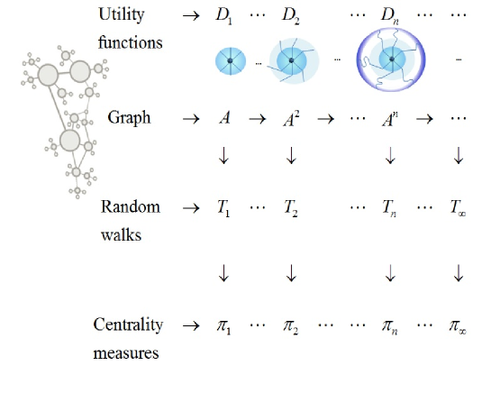
Figure 1: The ”astrological” equivalence partition of paths in a finite connected undirected graph (i.e., all paths of the given length $n$ starting at the same node are equivalent) induces the set of scale dependent random walks, the stationary distributions of which are the centrality measures accounting for the fractions of $n-$walks traversing a node.

The powers of adjacency matrix $A^{n}$ accounts for the numbers of paths of the length $n$ existed in the graph $G$, and the aggregated utility functions for each equivalence class is given by $D_{n}=\mathrm{diag}\left(\sum_{i=1}^{N}A^{n}_{1,i},\ldots,\sum_{i=1}^{N}A^{n}_{N,i}\right).$ We can define a set of stochastic transition matrices

$$T^{(n)}\,\,=\,\,D^{-1}_{n}A^{n},\quad n=1,\ldots\infty$$ (1)

that describe the discrete time Markov chains (the random walks) on the graph $G,$ in which all paths of length $n$ starting at the same node are considered equiprobable. Provided the adjacency matrix $A$ is irreducible, the Perron-Frobenius theorem (see, for example, Graham:87 ) states that its dominant eigenvalue $\alpha>0$ is simple, and the corresponding left and right eigenvectors can be chosen positive, $A\varphi=\alpha\varphi,$ $\varphi_{i}>0.$ As $n\to\infty,$ the elements of the transition matrices (1) tend to a constant row matrix,

$$T^{(\infty)}\,\,=\,\,\lim_{n\to\infty}\left(T^{(n)}\right)_{ij}\,\,=\,\,\left[\frac{\varphi_{i}}{\sum_{i\in\mathcal{V}}\varphi_{i}}\right]_{i=1,\ldots,N}\,\,=\,\,\lim_{n\to\infty}\left(\pi^{(n)}_{i}\right).$$ (2)

The elements of the left eigenvectors belonging to the biggest eigenvalue $\mu=1$ of the matrices $T^{(n)}$ are nothing else but the centrality measures Volchenkov:2013 defined as the fractions of $n$-walks traversing the node $i$,

$$\pi^{(n)}_{i}\,\,=\,\,\frac{\sum_{j\in\mathcal{V}}A^{n}_{i,j}}{\sum_{s,j\in\mathcal{V}}A^{n}_{s,j}}.$$ (3)

The first centrality measure,

$$\pi^{(1)}_{i}\,\,=\,\,\frac{\sum_{j\in\mathcal{V}}A_{i,j}}{\sum_{s,j\in\mathcal{V}}A_{s,j}}\,\,=\,\,\frac{\deg(i)}{2E},$$

where $\deg(i)$ is the degree of the node $i$ in $G,$ is the well-known stationary distribution of the nearest-neighbor random walks; the doubled number of edges $2E$ appears in that because of each edge can be traversed in both directions. The node centralities of the higher orders are increasingly sensitive to the proximity of the node to irregularities and defects of the graph.

To illustrate a dramatic dissimilarity of random walks at different scales $n$, we show the resulting densities of random walkers spreading during 100 iterations from the left lowest corner of the of the square $30\times 30$ containing a number of rectangular obstacles located along the main diagonal (see Fig. 2). In Fig. 21, we have presented a contour density plot for the the usual nearest neighbor random walk transition operator $T^{(1)}$, and Fig. 22 is for $T^{(10)}$.

1.)

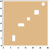
2.)

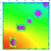
3.)

Figure 2: Two different random walks ($T^{(1)}$ and $T^{(10)}$) spread from the lower left corner of 1.) the square $30\times 30$ containing a number of obstacles located along the main diagonal. 2.) The contour density plot representing the density of random walkers spreading in accordance with the usual, nearest neighbor random walk transitions $T^{(1)},$ after 100 iterations. 3.) The contour density plot representing the density of random walkers spreading in accordance with the transitions to the 10-th neighbor $T^{(10)},$ after 100 iterations (the stationary distribution $\pi^{(10)}$ is already reached).

While the random walks $T^{(10)}$ have already reached the stationary distribution $\pi^{(10)}$ by $t=100,$ the usual, nearest neighbor random walks $T^{(1)}$ are still in spread toward an almost homogeneous distribution $\pi^{(1)}$ (which depend only upon the local connectivity of the cell, $\pi^{(1)}_{i}=\deg(i)/2E$) being less sensitive either to defects, or to the cage boundaries and covering all available space virtually uniformly, including the spaces between the obstacles. In contrast to them, the random walks $T^{(10)}$ are ”repelling” from obstacles, as the centrality measure $\pi^{(10)}$ quantifying the fraction of paths of the length $10$ traversing a square cell dramatically decreases in the vicinity of obstacles and boundaries, so that in the stationary distribution reached by $T^{(10)}$ the density of random walkers between the obstacles and along the boundaries appears to be minimal. In particular, they almost do not diffuse beyond the last obstacle, at the upper right corner of the square, and between the first obstacle and the cage boundary, at the lower left corner of the square (see Fig. 22).

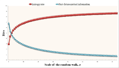
Figure 3: Left: The square $30\times 30$ containing a number of obstacles located along the main diagonal, the same we used in the previous simulation. Right: The entropy rate (marked by squares) and the past-future mutual information (marked by triangles) via the scale $n$ of the random walks defined in the square.

Since random walks at the different scales interfere with the structure differently, they can provide us with the important data on how a structure can store, organize, and transform information. It is obvious that the random walks of different scales $T^{(n)}$ are characterized by the different entropy rates,

$$H^{(n)}\,\,=\,\,-\sum_{i,j\in\mathcal{V}}\pi^{(n)}_{i}T^{(n)}_{ij}\log_{2}T^{(n)}_{ij},$$ (4)

indicating that the level of disorder in the random transitions within the given structure varies with the changing scale $n$. The complimentary information about the level of regularities or structural correlations observed at the different scales of the structure is given by the past-future mutual information (the excess entropy) introduced in Crutchfield:83 ; Shaw:1984 ,

$$C^{(n)}\,\,=\,\,\lim_{N\to\infty}\left(H^{(n)}(S^{N})-H^{(n)}\cdot N\right)\,\,=\,\,-\sum_{i\in\mathcal{V}}\pi^{(n)}_{i}\,\log_{2}\frac{\pi^{(n)}_{i}}{\,\,\prod_{j\in\mathcal{V}}\left(T^{(n)}_{ij}\right)^{T^{(n)}_{ij}}\,\,}.$$ (5)

where the block entropy is defined by

$$H^{(n)}(S^{N})\,\,=\,\,-\sum_{S^{N}}P^{(n)}(S^{N})\log_{2}P^{(n)}(S^{N}),$$ (6)

in which $P^{(n)}(S^{N})$ is the probability to find a path (a block of symbols identifying the path) $S^{N}$ of the length $N,$ in the random walks of the scale $n$. The second equality in (5) is due to the fact that the transition probability between states in a Markov chain is independent of $N$ and can be readily calculated ( see Li:1991 for details).

The excess entropy $C^{(n)}$ goes in literature by a number of different names (such as ”complexity”, Shaw:1984 ) as a measure of one type of the ”memory” that structure imposes on the process defined on that (in our case, the random walks, performing transitions of the scale $n$) and thus can serve as a measure of structural correlations presented in the environment Feldman:2008 . In Fig. 3 (Right), we have presented the entropy rates calculated accordingly to 4 and the past-future mutual information (the excess entropy) defined by 5, for the random walks of increasing scales defined on the square $30\times 30$ including a number of obstacles, the same as we used in the previous simulation (see Fig. 3 (Left)). As the scale of random walks increases, the level of transition randomness quantified by the entropy rate $H^{(n)}$ shows the almost logarithmic growth sketched on Fig. 3 (Right), gradually approaching its maximum for the maximum entropy random walks $T^{(\infty)}.$ At the same time, the behavior of the excess entropy $C^{(n)}$ is complimentary, decreasing from its maximal value attained for the nearest neighbor random walk (the maximal past-future mutual information, or the maximal complexity random walks) to the walks characterized by the minimal dependence on past path attained for the maximum entropy random walks $T^{(\infty)}.$

A.)
B.)
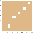
C.)

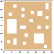
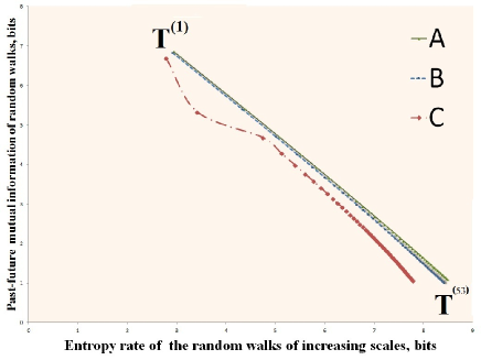
Figure 4: The complexity-entropy diagram shows the past-future mutual information (vertical axis) versus the entropy rate (horizontal axis), for the random walks of increasing scales $T^{(n)}$, for different environments: the environment (A) constitutes the $30\times 30$ square free of obstacles, the environment (B) contains five rectangular obstacles located along the diagonal of the square, the environment (C) contains 20 different rectangular obstacles distributed randomly over the available space.

It is clear that high order (i.e., low entropy) does not necessarily mean a highly correlated structure (i.e. high past-future mutual information). Obviously, the precise relation between the paces of the entropy rate and of the past-future mutual information (complexity) of transitions for the random walks across the different scales also depends upon the particular structural features of the environment. In the complexity-entropy diagram shown in Fig. 4(Right), we presented the past-future mutual information (vertical axis) versus the entropy rate (horizontal axis) for the random walks of increasing scales $T^{(n)}.$ The complexity-entropy diagram has been proposed by Crutchfield:83 and Feldman:2008 in order to demonstrate how the system stores, organizes, and transforms information. In our case, the diagram Fig. 4 (Right) indicates the complexity-entropy relationship for the random walks of increasing scales defined in three different rectangular environments of increasing structural complexity sown in Fig. 4 (Left). The environment (A) is free of obstacles, so that the difference between the centrality measures $\pi^{(n)}$ at the different scales comes merely from the boundary effects which do not essentially sound, especially for the random walks of not very large $n$. As a consequence, the complexity-entropy relation for the random walks defined in the environment (A) is almost linear, gradually deviating from linearity, for the large values of $n$. Therefore we can conclude that the relation between structure and order in the random transitions within an ”empty room” is straightforward across the different scales: the structure (provided by the walls, bounding the environment) reinforces the order. The next environment presented in Fig. 4 (Left) (B) is just the same that we used in the previous simulations; it contains five rectangular obstacles located along the diagonal of the square. As the number of obstacles increases, the centralities of cells with regard to the long paths decay dramatically, so that the departure from linearity in the complexity-entropy relation becomes even more visible, especially for the large values of $n$. Thus, we can say that in random transitions the strength of reinforcement of order by structure increases in presence of obstacles. This statement apparently holds true when the number of obstacles grows, yet other effects can come into play. Eventually, the last environment presented in Fig. 4 (Left) (C) contains 20 different rectangular obstacles distributed randomly over the available space. As we expected, the departure from linearity in the complexity-entropy relation increases for the environment (C), and an intriguing deviation also appears for $T^{(2)},$ determining the random walks based on the transitions to the second nearest neighbors. The inordinate drop of the past-future mutual information values producing the remarkable deviation of the complexity-entropy relation from linearity (see Fig. 4 (Right) (C)) for the short-range random walks obviously signifies the localization of random walkers inside the spaces formed by the filamentary sequences of the closely located obstacles. As we have already mentioned, the past-future mutual information quantifies the dependence of the forthcoming random transitions upon the past walk, and therefore the decay of that value indicates some extend of indifference of random transitions regarding the previous history, for the short-range walks. No matter how a random walker performing the short-range walk enters the locally quasi-bounded space, with the relatively high probability it remains trapped in that at least for a while.

In the next sections, we suppose that the random walk of a proper scale is chosen that eliminates the structural features of the environment or a database. We show how it is possible to geometrize the data with the use of the random walks.

3 Path integral distance and probabilistic geometry

The path integral formulation of quantum mechanics has been proposed by Richard Feynman as a description of quantum theory which generalizes the action principle of classical mechanic: the classical notion of a single, unique trajectory for a system is replaced in that with a sum, or functional integral, over an infinity of possible trajectories to compute a quantum amplitude called the propagator. The path integral also relates quantum and stochastic processes, as the Schrödinger equation is nothing else but a diffusion equation with an imaginary diffusion constant, and therefore the path integral is an analytic continuation of a method for summing up all possible random walks. The propagator resulted from the path integral calculation also can be viewed as the left inverse of the operator appropriate to the spread of particles, and is therefore considered to be the Green’s function of the Laplace operator describing the diffusion process. It is well known that if the kernel of the diffusion operator is non-trivial, then the Green’s function is not unique. However, in practice, the certain symmetry requirement imposed on the kernel will give a unique Green’s function. It is known that Green’s functions provide a powerful tool in dealing with a wide range of diffusion-type problems such as chip-firing games, load balancing algorithms, and the calculation of the so-called hitting time, the expected number of steps for a Markov chain to reach a state $y$ with an initial state $x$, Chung:2000 . Below, we briefly describe the Green’s function approach to random walks defined on graphs or databases, following Volchenkov:2011 ; Volchenkov:2013 .

Given a random walk defined by a transition matrix $T$ on a finite connected undirected weighted graph $G(\mathcal{V},\mathcal{E})$, all vertices and their subsets can be characterized by certain probability distributions and characteristic times Volchenkov:2011 . The stationary distribution of random walks (the left eigenvector of the transition matrix $T$ belonging to the maximal eigenvalue $\mu=1$) determines a unique measure on $\mathcal{V}$ with respect to which the transition operator $T$ becomes self-adjoint and is represented by a symmetric transition matrix $\widehat{T}.$ The use of self-adjoint operators (such as the normalized graph Laplacian) becomes now standard in spectral graph theory Chung:1997 and in studies devoted to random walks on graphs Lovasz:1993 . Diagonalizing the symmetric matrix $\widehat{T}$, we obtain $\widehat{T}={\Psi}{M}{\Psi}^{\top},$ where ${\Psi}$ is an orthonormal matrix, ${\Psi}^{\top}={\Psi}^{-1},$ and $M$ is a diagonal matrix with entries $1=\mu_{1}>\mu_{2}\geq\ldots\geq\mu_{N}>-1$ (here, we do not consider bipartite graphs, for which $\mu_{N}=-1$). The rows ${\psi}_{k}=\left\{\psi_{k,1},\ldots,\psi_{k,N}\right\}$ of the orthonormal matrix ${\Psi}$ are the real eigenvectors of $\widehat{T}$ that forms an orthonormal basis in Hilbert space $\mathcal{H}(\mathcal{V}),$ ${\psi}_{k}:\mathcal{V}\to S_{1}^{N-1},$ $k=1,\ldots N$, where $S_{1}^{N-1}$ is the $N-1$-dimensional unit sphere. We consider the eigenvectors ${\psi}_{k}$ ordered in accordance to the eigenvalues they belong to. For eigenvalues of algebraic multiplicity $m>1$, a number of linearly independent orthonormal ordered eigenvectors can be chosen to span the associated eigenspace. The first eigenvector ${\psi}_{1}$ belonging to the largest eigenvalue $\mu_{1}=1$ (which is simple) is the Perron-Frobenius eigenvector that determines the stationary distribution of random walks over the graph nodes, $\psi_{1,i}^{2}=\pi_{i}.$

The diffusion process is described by the irreducible Laplace operator ${L}={1}-{T}$ which has the one-dimensional null space spanned by the vector $\pi.$ As being a member of the multiplicative group under the ordinary matrix multiplication Erdelyi:1967 ; Meyer:1975 , the Laplace operator possesses a group inverse (a special case of Drazin inverse, Drazin:1958 ; Ben-Israel:2003 ; Meyer:1975 ) with respect to this group, $L^{\sharp},$ which satisfies the following conditions Erdelyi:1967 :

$${LL}^{\sharp}{L}={L},\quad{L}^{\sharp}{LL}^{\sharp}={L}^{\sharp},\quad\mathrm{and}\quad\left[{L},{L}^{\sharp}\right]=0,$$

where $[{A},{B}]={AB}-{BA}$ denotes the commutator of matrices. The last condition implies that ${L}^{\sharp}$ shares the same set of symmetries as the Laplace operator, being the Green function of the diffusion equation. The methods for computing the group generalized inverse for matrices of $\mathrm{rank}({L})=N-1$ have been developed in Robert:1968 ; Campbell:1976 and by many other authors. Perhaps, the most elegant way is by considering the eigenprojection of the matrix $L$ corresponding to the eigenvalue $\lambda_{1}=1-\mu_{1}=0$ developed in Campbell:1976 ; Hartwig:1976 ; Agaev:2002 ,

$${L}^{\sharp}\,\,=\,\,\left({L}+{Z}\right)^{-1}-{Z},\quad{Z}\,\,=\,\,\prod_{\lambda_{i}\neq 0}\left({1}-L/{\lambda_{i}}\right),\quad\lambda_{i}\,\,=\,\,1-\mu_{i}$$ (7)

where the product in the idempotent matrix ${Z}$ is taken over all nonzero eigenvalues $\lambda_{i>1}$ of $L.$ The eigenprojection (7) can be considered as a stereographic projection that projects the points ${\psi}_{k}$ on the sphere $S_{1}^{N-1}$ to a projective manifold such that all vectors collinear to the vector $\psi_{1}$ (corresponding to the stationary distribution of random walks) are projected onto a common image point. Since $\psi_{1,i}\equiv\sqrt{\pi_{i}}>0$ for any $i\in\mathcal{V},$ we can define the new basis vectors $\left\{\psi^{\prime}_{k}\right\}_{k=1}^{N},$ spanning the projection space $\mathrm{P}\mathbb{R}_{\pi}^{(N-1)},$ such that $\psi^{\prime}_{k}=\left(1,{\psi_{2,i}}/{\psi_{1,i}},\ldots,{\psi_{N,i}}/{\psi_{1,i}}\right).$ We define the inner product between any two vectors $\xi,\zeta\in\mathbb{R}^{N}$ by

$$\left(\xi,\zeta\right)_{T}\,\,=\,\,\left(\xi,{L}^{\sharp}\zeta\right).$$ (8)

The inner product (8) is a symmetric real valued scalar function that allows us to define the (squared) norm of a vector $\xi$ by

$$\left\|\,\xi\,\right\|^{2}_{T}\,\,=\,\,\left(\xi,{L}^{\sharp}\xi\right)$$ (9)

and an angle $\theta\in[0,180^{\mathrm{o}}]$ between two vectors,

$$\theta\,\,=\,\,\arccos\left(\frac{\left(\xi,\zeta\right)_{T}}{\left\|\,\xi\,\right\|_{T}\left\|\,\zeta\,\right\|_{T}}\right).$$ (10)

The Euclidean distance between two vectors is given by

$$\left\|\xi-\zeta\right\|^{2}_{T}\,\,=\,\,\left\|\,\xi\,\right\|^{2}_{T}+\left\|\,\zeta\,\right\|^{2}_{T}-2\left(\xi,\zeta\right)_{T}.$$ (11)

For instance, let us consider the vector (distribution) $\mathbf{e}_{i}=\{0,\ldots 1_{i},\ldots 0\}$ pointing at the vertex $i$ of the graph $G$ in the canonical basis. The spectral representation of the generalized inverse for undirected graphs Volchenkov:2011 is given by

$${L}^{\sharp}_{i,j}\,\,=\,\,\sum_{k=2}^{N}\frac{1}{\lambda_{k}}\frac{\psi_{i,k}}{\psi_{i,1}}\frac{\psi_{j,k}}{\psi_{j,1}},\quad i,j=1,\ldots,N,$$ (12)

in which $\lambda_{k}$ are all nontrivial eigenvalues of the Laplace operator. The matrix (12) is real symmetric semi-positive, as its smallest eigenvalue $\Lambda_{1}=0.$ Accordingly (9), the spectral representation for the squared norm of $\mathrm{e}_{i}$ equals

$$f_{i}\,\,=\,\,\left\|\,\mathrm{e}_{i}\,\right\|_{T}^{2}\,=\,\frac{1}{\pi_{i}}\,\sum_{s=2}^{N}\,\frac{\,\psi^{2}_{s,i}\,}{\,\lambda_{s}\,}.$$ (13)

In the theory of random walks on undirected graphs Lovasz:1993 , the latter result is known as the spectral representation of the first passage time to the node $i\in\mathcal{V}$, the expected number of steps required to reach the node $i$ for the first time (i.e. without visiting any node twice) starting from a node randomly chosen among all nodes of the graph accordingly to the stationary distribution $\pi$. It is important to mention that the norm (9) of the stationary distribution $\pi$ equals zero,

$$\begin{array}[]{ll}f_{\pi}\,\,=\,\,\left\|\psi_{1}^{2}\right\|_{T}^{2}&=\sum_{i=1}^{N}\psi_{1,i}^{2}\sum_{1,j}^{N}\psi_{1,j}^{2}\sum_{\alpha=2}^{N}\frac{1}{\lambda_{\alpha}}\frac{\psi_{\alpha,i}}{\psi_{1,i}}\frac{\psi_{\alpha,j}}{\psi_{1,j}}\\ &=\sum_{\alpha=2}^{N}\frac{1}{\lambda_{\alpha}}\underbrace{\sum_{j=1}^{N}\psi_{1,j}\psi_{\alpha,j}}_{0}\underbrace{\sum_{i=1}^{N}\psi_{1,i}\psi_{\alpha,i}}_{0}=0,\end{array}$$ (14)

due to the orthogonality of eigenvectors $\psi_{k}$.

The Euclidean distance between any two nodes of the graph induced by the random walk,

$$K_{i,j}\,=\,\left\|\,\mathrm{e}_{i}-\mathrm{e}_{j}\,\right\|^{2}_{T}\,=\,\sum_{s=2}^{N}\,\frac{1}{\lambda_{s}}\left(\frac{\psi_{s,i}}{\sqrt{\pi_{i}}}-\frac{\psi_{s,j}}{\sqrt{\pi_{j}}}\right)^{2},$$ (15)

is nothing else but the commute time, the expected number of steps required for a random walker starting at $i$ to visit $j$ and then to return back to $i$, without visiting any node twice Lovasz:1993 . The commute time can be represented as a sum, $K_{i,j}=H_{i,j}+H_{j,i}$, in which

$$H_{i,j}\,\,=\,\,\left\|\,\mathrm{e}_{i}\,\right\|^{2}_{T}-\left(\,\mathrm{e}_{i},\mathrm{e}_{j}\,\right)_{T}$$ (16)

is the first-hitting time which is the expected number of steps a random walker starting from the node $i$ needs to reach $j$ for the first time, Lovasz:1993 . The first-hitting time satisfies the equation

$$H_{ij}\,=\,1+\sum_{i\sim v}H_{vj}T_{vi}$$ (17)

reflecting the fact that the first step takes a random walker to a neighbor $v\,\in\,V$ of the starting node $i\,\in\,V$, and then it has to reach the node $j$ from there. In principle, the latter equation can be directly used for computing of the first-hitting times, however, $H_{ij}$ are not the unique solutions of (17); the correct definition requires an appropriate diagonal boundary condition, $H_{ii}=0$, for all $i\,\in\,V$, Lovasz:1993 .

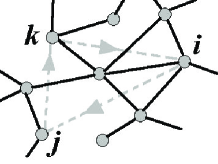
Figure 5: The triangle symmetry of the first-hitting times: the sum of first-hitting times calculated for random walks defined by the transition operator of nearest-neighbor random walks visiting any three nodes $i$, $j$, and $k$, equals to the sum of the first-hitting times in the reversing direction.

The zero-diagonal matrix of first-hitting times is not symmetric, $H_{i,j}\neq H_{j,i}$, even for a regular graph. However, a deeper triangle symmetry property (see Fig. 5) has been observed in Coopersmith:1993 for random walks defined by the transition operator of nearest-neighbor random walks. Namely, for every three nodes in the graph, the consecutive sums of the first-hitting times in the clockwise and in the counterclockwise directions are equal,

$$H_{ij}+H_{jk}+H_{ki}\,=\,H_{ik}+H_{kj}+H_{ji}.$$ (18)

We can now use the first-hitting times in order to quantify the accessibility of nodes and subgraphs for random walkers. Its average with respect to the first index equals the first-passage time to the node,

$$f_{j}\,\,=\,\,\left\|\mathrm{e}_{j}\right\|_{T}^{2}\,\,=\,\,\sum_{i\in\mathcal{V}}\pi_{i}H_{i,j}.$$ (19)

It is worth a mention that matrix (12) can be considered as the Gram matrix, $L^{\sharp}=\left({\mathbf{q}}_{i},{\mathbf{q}}_{j}\right)_{P\mathbb{R}^{(N-1)}},$ with respect to the usual dot product of vectors in the projection space $P\mathbb{R}^{(N-1)}.$ The vector

$${\mathbf{q}}_{i}\,\,=\,\,\left\{\frac{1}{\sqrt{\lambda_{2}}}\frac{\psi_{2,i}}{\psi_{1,i}},\ldots,\frac{1}{\sqrt{\lambda_{N}}}\frac{\psi_{N,i}}{\psi_{1,i}}\right\}$$ (20)

represents an image of the vertex $i\in\mathcal{V}$ in the projection space $P\mathbb{R}^{(N-1)}.$ The image of the graph $G(\mathcal{V},\mathcal{E})$ in the projection space $P\mathbb{R}^{(N-1)}$ constitutes a diffusion manifold of self-avoiding random walks (in which nodes cannot be visited twice) in affine subspace, as we can subtract vertices (by component wise subtracting of their images (20)) to get vectors, or add a vector to a vertex to get another vertex, but we cannot add new vertices. It seems natural to describe the structural properties of the graph using the topology of the manifold of self-avoiding diffusion in the projection space $P\mathbb{R}^{(N-1)}.$ The scalar product $\left(\mathbf{e}_{i},\mathbf{e}_{j}\right)_{P\mathbb{R}^{(N-1)}}$ estimates the expected overlap of random paths toward the nodes $i$ and $j$ starting from a node randomly chosen in accordance with the stationary distribution of random walks $\pi$ Volchenkov:2011 . The normalized expected overlap of random paths given by the cosine of an angle (10) calculated in the $(N-1)-$dimensional Euclidean space associated to random walks has the structure of Pearson’s coefficient of linear correlations that reveals it’s natural statistical interpretation. If the cosine of (10) is close to 1, the expected random paths toward the both nodes are mostly identical. The value of cosine is close to -1 if the walkers share the same random paths but in the opposite direction. Finally, the correlation coefficient equals 0 if the expected random paths toward the nodes do not overlap at all.

4 Maze of labyrinths

It is believed that once upon a time labyrinths had served as traps for malevolent spirits or as defined paths for ritual dances (there are surviving descriptions of French clerics performing a ritual Easter dance along the path on Easter Sunday Kern:2000 ). The present-day notion of a labyrinth is a place where one can lose his way, a confusing path, hard to follow without a thread, a intricate and inextricable path to the home of a sacred ancestor Schuster:1996 . Being a symbol of ambiguity and disorientation, the notion of a labyrinth is also used to describe a confusing logic of arguments. In Plato’s dialogue Euthydemus, Socrates describes the labyrinth in the line of a logical argument:

”Then it seemed like falling into a labyrinth: we thought we were at the finish, but our way bent round and we found ourselves as it were back at the beginning, and just as far from that which we were seeking at first.”

It is interesting to discuss the general structural properties of labyrinths that make them so difficult to navigate in and, at the same time, so mysteriously attractive to our minds. In Fig. 6 (left), we have presented the maze consisting of 45 interconnected rectangles providing the space for motion and displayed its spatial graph representing the connectivity pattern.

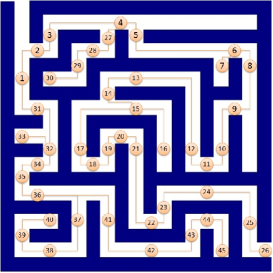
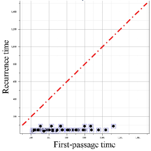
Figure 6: Left: the maze consisting of 45 interconnected rectangles providing the space for motion, along its spatial graph representing the connectivity pattern. Right: the recurrence times to all 45 rectangular spaces of the maze via the first-passage times to them (both characteristic times are calculated with regard to the nearest-neighbor random walks). The dash-dotted reference line ($x=y$) indicates the equality.

It is known that for a stationary, discrete-valued stochastic process the expected recurrence time to return to a state is the reciprocal of the probability of this state, Kac:1947 . The expected recurrence time to a node which indicates how long a random walker must wait to revisit the site is inverse proportional to the stationary distribution, $\pi_{i}$,

$$r_{i}\,\,=\,\,\frac{1}{\,\pi_{i}\,}\,\,=\,\,\frac{1}{\,\psi^{2}_{1,i}\,}.$$ (21)

It follows from the spectral representation of the first-passage time (13) that they are proportional to each other,

$$f_{i}\,\,=\,\,\left\|{\bf e}_{i}\right\|^{2}_{T}\,\,=\,\,\frac{1}{\psi^{2}_{1,i}}\sum_{k=2}^{N}\frac{\psi^{2}_{k,i}}{\lambda_{k}}\,\,=\,\,r_{i}\cdot\sum_{k=2}^{N}\frac{\psi^{2}_{k,i}}{\lambda_{k}},$$ (22)

where the proportionality coefficient can broadly vary. In particular, for the nearest-neighbor random walks, it can be seen from the Fig. 6(Right) that the first-passage times to places in mazes are systematically longer than the recurrence times to them. Although it may take a quite long time for a random walker to reach a place for the first time, the walker is doomed to revisit this place again and again, as the recurrence time to that might be quite short, as being determined (for the the nearest-neighbor random walks) merely by the local connectivity of the place (that might be quite high), but not by the integral features relating the place to the global structure of the environment. In fact, the random walker appears to be trapped within the maze environment and might find it confusing. In Fig. 6(Right), we can see that with respect to the overall structure of the maze, all spaces of movement (rectangles) constitute such the traps (as the first-passage times to all of them substantially exceed the recurrence times). It is clear that movements of a real human traveler are rather self-determined than random. However, as we have discussed in Sec. 2, the interpretation of a place with respect to the overall structure of the environment can be based on some random walks defined in that. In particular, the nearest-neighbor random walks are found practically efficient for the prediction of human navigation in urban environnements Blanchard:2009 (see also Sec. 6). In the forthcoming sections, we show that random walks can certainly inform us about the intelligibility of environments (lucidly indicated by the relative land prices) and tonality of music melodies.

5 Can we hear first-passage times?

A system for using dice to compose music randomly, without having to know neither the techniques of composition, nor the rules of harmony, named Musikalisches Würfelspiel - Musical dice game (MDG) had become quite popular throughout Western Europe in the $18^{th}$ century Noguchi:1996 . Depending upon the results of dice throws, the certain pre-composed bars of music were patched together resulting in different, but similar, musical pieces. ”The Ever Ready Composer of Polonaises and Minuets” was devised by Ph. Kirnberger, as early as in 1757. The famous chance music machine attributed to W.A. Mozart (K 516f) consisted of numerous two-bar fragments of music named after the different letters of the Latin alphabet and destined to be combined together either at random, or following an anagram of your beloved had been known since 1787.

We can consider a note as an elementary event providing a natural discretization of musical phenomena that facilitate their performance and analysis. Namely, given the entire keyboard $\mathcal{K}$ of 128 notes (standard for the MIDI representations of music) corresponding to a pitch range of 10.5 octaves, each divided into 12 semitones, we regard a note as a discrete random variable $X$ that maps the musical event to a value of a $R$-set of pitches $\mathcal{P}=\{x_{1},\ldots,x_{R}\}\subseteq\mathcal{K}.$ In the musical dice game, a piece is generated by patching notes $X_{t}$ taking values from the set of pitches $\mathcal{P}$ that sound good together into a temporal sequence $\left\{X_{t}\right\}_{t\geq 1}$. Herewith, two consecutive notes, in which the second pitch is a harmonic of the first one are considered to be pleasing to the ear, and therefore can be patched to the sequence. Harmony is based on consonance, a concept whose definition changes permanently in musical history. Two or more notes may sound consonant for various reasons such as luck of perceptual roughness, spectral similarity of the sequence to a harmonic series, familiarity of the sound combination in contemporary musical contexts, and eventually for a personal taste, as there are consonant and dissonant harmonies, both of which are pleasing to the ears of some and not others. A detailed statistical analysis of subtle harmony conveyed by melodic lines in tonal music certainly calls for the complicated stochastic models, in which successive notes in the sequence $\left\{X_{t}\right\}_{t\geq 1}$ are not chosen independently, but their probabilities depend on preceding notes. In the general case, a set of $n$-note probabilities $\Pr\left[X_{t+1}=x\mid X_{t}=y,X_{t-1}=z,\ldots,X_{t-n}=\upsilon\right]$ might be required to insure the resemblance of the musical dice games to the original compositions. However, it is rather difficult to decide a priori upon the enough memory depth $n$ in the stochastic models required to compare reliably the pieces of tonal and atonal music created by different composers, with various purposes, in different epochs, for diverse musical instruments subjected to the dissimilar tuning techniques. Under such circumstances, it is mandatory to identify some meaningful blocks of musical information and to detect the hierarchical tonality (basic for perception of harmony in Western music Dahlhaus:2007 ) in a simplified statistical model, as the first step of statistical analysis. For this purpose, in the present work, we neglect possible statistical influences extending over than the only preceding note and limit our analysis to the simplest time – homogeneous Markov chain,

$$\Pr\left[X_{t+1}=x\mid X_{t}=y,X_{t-1}=z,\ldots\right]\,=\,\Pr\left[X_{t+1}=x\mid X_{t}=y\right]\,=\,T_{yx},$$ (23)

where the elements of the stochastic transition matrix $T_{yx},$ $\sum_{x\in\mathcal{P}}T_{yx}=1,$ weights the chance of a pitch $x$ going directly to another pitch $y$ independently of time. It is worth mentioning that the model (23) obviously does not impose a severe limitation on melodic variability, since there are many possible combinations of notes considered consonant, as sharing some harmonics and making a pleasant sound together. The relations between notes in (23) are rather described in terms of probabilities and expected numbers of random steps than by physical time. Thus the actual length $N$ of a composition is formally put $N\to\infty,$ or as long as you keep rolling the dice. The examples of transition matrices generated for the different musical compositions are shown in Fig. 7. They appear to be essentially not symmetric: if $T_{xy}>0,$ for some $x,y,$ it might be that $T_{yx}=0.$ A musical composition can be represented by a weighted directed graph, in which vertices are associated with pitches and directed edges connecting them are weighted accordingly to the probabilities of the immediate transitions between those pitches. Markov’s chains determining random walks on such graphs are not ergodic: it may be impossible to go from every note to every other note following the score of the musical piece.

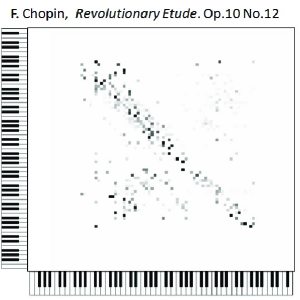
Figure 7: Transition matrices for the MDG based on the F.Chopin ”Revolutionary Etude” (Op.10, No 12) (left) and the I. Stravinsky ”The Fire-bird” suite (right).

In music theory Thomson:1999 , the hierarchical pitch relationships are introduced based on a tonic key, a pitch which is the lowest degree of a scale and that all other notes in a musical composition gravitate toward. A successful tonal piece of music gives a listener a feeling that a particular (tonic) chord is the most stable and final. The regular method to establish a tonic through a cadence, a succession of several chords which ends a musical section giving a feeling of closure, may be difficult to apply without listening to the piece.

While in a MDG, the intuitive vision of musicians describing the tonic triad as the ”center of gravity” to which other chords are to lead acquiers a quantitative expression. Every pitch in a musical piece is characterized with respect to the entire structure of the Markov chain by its level of accessibility estimated by the first passage time to it Volchenkov:2011 that is the expected length of the shortest path of a random walk toward the pitch from any other pitch randomly chosen over the musical score. Analyzing the first passage times in scores of tonal musical compositions, we have found that they can help in resolving tonality of a piece, as they precisely render the hierarchical relationships between pitches. It is interesting to note that from the physical point of view the first passage time can be naturally interpreted as a potential, as being equal to the diagonal elements of the generalized inverse of the Laplace operator. For example, the first passage time to a node precisely equals to the electric potential of the node, in an electric resistance network Volchenkov:2011 . Thus, in the framework of musical dice games, the role of a note in a tonal scale can be understood as its potential.

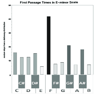
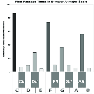
Figure 8: The histograms show the first passage times to the notes for the MDG over a part of Duet I of J.S. Bach (BWV 802) written in E minor (left) and over a part of the Cello Sonata No.3, Op.69 of L.V. Beethoven written in E major, A major (right) mapped into a single octave. Bars are shaded with the intensity of gray scale $[0-100\%]$, in proportion to the magnitude of the first passage time. Therefore, the basic pitches of a tonal scale are rendered with light gray color, as being characterized by short first passage times, and the tonic key by the smallest magnitude of all.

The majority of tonal music assumes that notes spaced over several octaves are perceived the same way as if they were played in one octave Burns:1999 .

Using this assumption of octave equivalency, we can chromatically transpose each musical piece into a single octave getting the $12\times 12$ transition matrices, uniformly for all musical pieces, independently of the actual number of pitches used in the composition. Given a stochastic matrix ${\bf T}$ describing transitions between notes within a single octave $\mathcal{O}$, the first passage time to the note $i\in\mathcal{O}$ is computed in Volchenkov:2011 .

We have shown in Fig. 8 the two examples of the arrangements of first passage times to notes in one octave, for the E minor scale (left) and E major, A major scales (right). The basic pitches for the E minor scale are E, F#, G, A, B, C, and D. The E major scale is based on E, F#, G#, A, B, C#, and D#. Finally, the A major scale consists of A, B, C#, D, E, F#, and G#. The values of first passage times are strictly ordered in accordance to their role in the tone scale of the musical composition. Herewith, the tonic key is characterized by the shortest first passage time (usually ranged from 5 to 7 random steps), and the values of first passage times to other notes collected in ascending order reveal the entire hierarchy of their relationships in the musical scale.

It is intuitive that the time of recurrence to a note estimated by $\pi_{i}^{-1}$ is related positively to the first passage time to it, $\mathcal{F}_{i}$: the faster a random walk over the score hits the pitch for the first time, the more often it might be expected to occur again. The time of recurrence equals the first passage time in a salient recurring succession of notes (a motif) - the pattern of three short notes followed by one long that opens the Fifth Symphony of L.V. Beethoven and reappears throughout the work is a classic example.

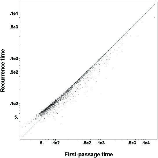
Figure 9: The log-log scatter plot contains $12\times 804$ points representing the recurrence time vs. the first passage time to the $12$ notes of one octave, over the MDG based on $804$ compositions of $29$ composers. The straight line is given for a reference indicating the horizon of intelligibility (when equality of recurrence times and first passage times is achieved); departures from linearity signify departures from intelligibility.

The log-log scatter plot shown in Fig. 9 represents the relation between the recurrence time and the first passage time to the $12$ notes of one octave in all MDG over musical compositions we studied. The straight line indicates equality of recurrence times and first passage times. The data provide convincing evidence for the systematic departure of recurrence times from first passage times for those pitches characterized by the relatively short first passage times (recurrence times to them are typically longer than first passage times). The excess of recurrence times over first passage times quantifies musical development encompassing distinct musical figures that are subsequently altered and sequenced throughout a piece of music. It is not a surprise that such a musical development is essentially visible in the range of the relatively short first passage times, as they play an important role in the tonal scale structure of a piece guaranteeing its unity.

6 Can we see first-passage times?

A belief in the influence of the built environment on humans was common in architectural and urban thinking for centuries. Cities generate more interactions with more people than rural areas because they are central places of trade that benefit those who live there. People moved to cities because they intuitively perceived the advantages of urban life. City residence brought freedom from customary rural obligations to lord, community, or state and converted a compact space pattern into a pattern of relationships by constraining mutual proximity between people. Spatial organization of a place has an extremely important effect on the way people move through spaces and meet other people by chance, Hillier:1984 ; Blanchard:2009 . Compact neighborhoods can foster casual social interactions among neighbors, while creating barriers to interaction with people outside a neighborhood. The phenomenon of clustering of minorities, especially that of newly arrived immigrants, is well documented Wirth . Clustering is considering to be beneficial for mutual support and for the sustenance of cultural and religious activities. At the same time, clustering and the subsequent physical segregation of minority groups would cause their economic marginalization. The spatial analysis of the immigrant quarters Vaughan01 and the study of London’s changes over 100 years Vaughan02 shows that they were significantly more segregated from the neighboring areas, in particular, the number of street turning away from the quarters to the city centers were found to be less than in the other inner-city areas being usually socially barricaded by railways, canals and industries. It has been suggested Language that space structure and its impact on movement are critical to the link between the built environment and its social functioning. Spatial structures creating a local situation in which there is no relation between movements inside the spatial pattern and outside it and the lack of natural space occupancy become associated with the social misuse of the structurally abandoned spaces.

In traditional urban researches, the dynamics of an urban pattern come from the landmasses, the physical aggregates of buildings delivering place for people and their activity. The relationships between certain components of the urban texture are often measured along streets and routes considered as edges of a planar graph, while the traffic end points and street junctions are treated as nodes. Such a primary graph representation of urban networks is grounded on relations between junctions through the segments of streets. The usual city map based on Euclidean geometry can be considered as an example of primary city graphs. In space syntax theory (see Hillier:1984 ), built environments are treated as systems of spaces of vision subjected to a configuration analysis. Being irrelevant to the physical distances, spatial graphs representing the urban environments are removed from the physical space. It has been demonstrated in multiple experiments that spatial perception shapes peoples understanding of how a place is organized and eventually determines the pattern of local movement, Hillier:1984 . The decomposition of urban spatial networks into the complete sets of intersecting open spaces can be based on a number of different principles. In Jiang:2004 , while identifying a street over a plurality of routes on a city map, the named-street approach has been used, in which two different arcs of the primary city network were assigned to the same identification number (ID) provided they share the same street name.

Being interested in the interpretation of urban space by pedestrians, in the present paper, we take a ”named-streets”-oriented point of view on the decomposition of urban spatial networks into the complete sets of intersecting open spaces following our previous works Volchenkov:2007a ; Volchenkov:2007b . Being interested in the statistics of random walks defined on spatial networks of urban patterns, we assign an individual street ID code to each continuous segment of a street. The spatial graph of urban environment is then constructed by mapping all edges (segments of streets) of the city map shared the same street ID into nodes and all intersections among each pair of edges of the primary graph into the edges of the secondary graph connecting the corresponding nodes. We assign an individual ID code to each continuous segment of a street or a channel. The spatial graph of urban environment is then constructed by mapping all edges (segments of streets) of the city map shared the same street ID into nodes and all intersections among each pair of edges of the primary graph into the edges of the secondary graph connecting the corresponding nodes.

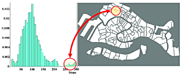
Figure 10: The Venetian Ghetto jumped out as by far the most isolated, despite being apparently well connected to the rest of the city.

We have analyzed the first-passage times to individual canals in the spatial graph of the canal network in Venice. The distribution of numbers of canals over the range of the first–passage time values is represented by a histogram shown in Fig. 10 (left). The height of each bar in the histogram is proportional to the number of canals in the canal network of Venice for which the first–passage times fall into the disjoint intervals (known as bins). Not surprisingly, the Grand Canal, the giant Giudecca Canal and the Venetian lagoon are the most connected. In contrast, the Venetian Ghetto (see Fig. 10 (right)) – jumped out as by far the most isolated, despite being apparently well connected to the rest of the city – on average, it took 300 random steps to reach, far more than the average of 100 steps for other places in Venice.

The Ghetto was created in March 1516 to separate Jews from the Christian majority of Venice. It persisted until 1797, when Napoleon conquered the city and demolished the Ghetto’s gates. Now it is abandoned.

The notion of isolation acquires the statistical interpretation by means of random walks. The first-passage times in the city vary strongly from location to location. Those places characterized by the shortest first-passage times are easy to reach while very many random steps would be required in order to get into a statistically isolated site.

Being a global characteristic of a node in the graph, the first-passage time assigns absolute scores to all nodes based on the probability of paths they provide for random walkers. The first-passage time can therefore be considered as a natural measure of statistical isolation of the node within the graph, Blanchard:2009 .

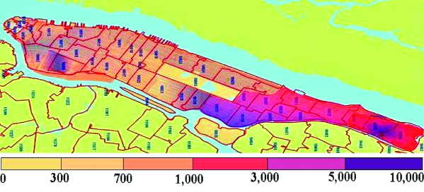
Figure 11: Isolation map of Manhattan. Isolation is measured by first-passage times to the places. Darker color corresponds to longer first-passage times.

A visual pattern displayed on Fig. 11 represents the pattern of structural isolation (quantified by the first-passage times) in Manhattan (darker color corresponds to longer first-passage times). It is interesting to note that the spatial distribution of isolation in the urban pattern of Manhattan (Fig. 11) shows a qualitative agreement with the map of the tax assessment value of the land in Manhattan reported by B. Rankin (2006) in the framework of the RADICAL CARTOGRAPHY project being practically a negative image of that.

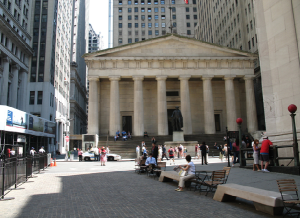
1).		2).
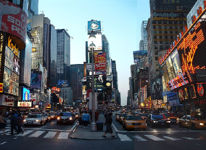
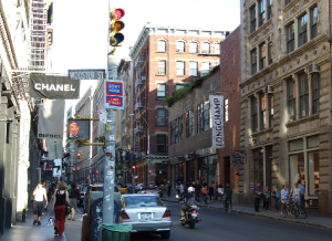
3).		4).
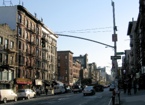
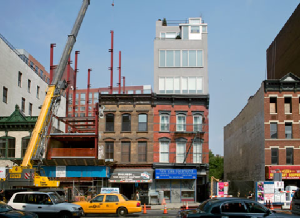
5).		6).

Figure 12: The first passage times in the borough of Manhattan, NYC: 1). the Federal Hall National Memorial $\sim$ 10 steps; 2). the Times square $\sim$ 100 steps; 3). the SoHo neighborhood, in Lower Manhattan $\sim$ 500 steps; 4). the East Village neighborhood, lying east of Greenwich Village, south of Gramercy and Stuyvesant Town $\sim$ 1,000 steps; 5). the Bowery neighborhood, in the southern portion of the New York City borough of Manhattan $\sim$ 5,000 steps; 6). the East Harlem (Spanish Harlem, El Barrio), a section of Harlem located in the northeastern extremity of the borough of Manhattan $\sim$ 10,000 steps;

The first-passage times enable us to classify all places in the spatial graph of Manhattan into four groups accordingly to the first-passage times to them Blanchard:2009 . The first group of locations is characterized by the minimal first-passage times; they are probably reached for the first time from any other place of the urban pattern in just 10 to 100 random navigational steps (the heart of the city), see Fig. 121 and Fig. 122. These locations are identified as belonging to the downtown of Manhattan (at the south and southwest tips of the island) – the Financial District and Midtown Manhattan. It is interesting to note that these neighborhoods are roughly coterminous with the boundaries of the ancient New Amsterdam settlement founded in the late 17^th century. Both districts comprise the offices and headquarters of many of the city’s major financial institutions such as the New York Stock Exchange and the American Stock Exchange (in the Financial District). Federal Hall National Memorial is also encompassed in this area that had been anchored by the World Trade Center until the September 11, 2001 terrorist attacks. We might conclude that the group of locations characterized by the best structural accessibility is the heart of the public process in the city.

The neighborhoods from the second group (the city core) comprise the locations that can be reached for the first time in several hundreds to roughly a thousand random navigational steps from any other place of the urban pattern (Fig. 123 and Fig. 124). SoHo (to the south of Houston Street), Greenwich Village, Chelsea (Hell’s Kitchen), the Lower East Side, and the East Village are among them – they are commercial in nature and known for upscale shopping and the ”Bohemian” life-style of their dwellers contributing into New York’s art industry and nightlife.

The relatively isolated neighborhoods such as Bowery (Fig. 125), some segments in Hamilton Heights and Hudson Heights, Manhattanville (bordered on the south by Morningside Heights), TriBeCa (Triangle Below Canal) and some others can be associated to the third structural category as being reached for the first time from 1,000 to 3,000 random steps starting from a randomly chosen place in the spatial graph of Manhattan. Interestingly, that many locations belonging to the third structural group comprises the diverse and eclectic mix of different social and religious groups. Many famous houses of worship had been established there during the late 19^th century – St. Mary’s Protestant Episcopal Church, Church of the Annunciation, St. Joseph’s Roman Catholic Church, and Old Broadway Synagogue in Manhattanville are among them. The neighborhood of Bowery in the southern portion of Manhattan had been most often associated with the poor and the homeless. From the early 20^th century, Bowery became the center of the so called ”b’hoy” subculture of working-class young men frequenting the cruder nightlife. Petty crime and prostitution followed in their wake, and most respectable businesses, the middle-class, and entertainment had fled the area. Nowadays, the dramatic decline has lowered crime rates in the district to a level not seen since the early 1960s and continue to fall. Although zero-tolerance policy targeting petty criminals is being held up as a major reason for the crime combat success, no clear explanation for the crime rate fall has been found.

The last structural category comprises the most isolated segments in the city mainly allocated in the Spanish and East Harlems. They are characterized by the longest first-passage times from 5,000 to 10,000 random steps (Fig. 126). Structural isolation is fostered by the unfavorable confluence of many factors such as the close proximity to Central Park (an area of 340 hectares removed from the otherwise regular street grid), the boundness by the strait of Harlem River separating the Harlem and the Bronx, and the remoteness from the main bridges (the Triborough Bridge, the Willis Avenue Bridge, and the Queensboro Bridge) that connect the boroughs of Manhattan to the urban arrays in Long Island City and Astoria. Many social problems associated with poverty from crime to drug addiction have plagued the area for some time. The haphazard change of the racial composition of the neighborhood occurred at the beginning of the 20^th century together with the lack of adequate urban infrastructure and services fomenting racial violence in deprived communities and made the neighborhood unsafe – Harlem became a slum. The neighborhood had suffered with unemployment, poverty, and crime for quite long time and even now, despite the sweeping economic prosperity and redevelopment of many sections in the district, the core of Harlem remains poor.

Recently, we have discussed in Volchenkov:2011 that distributions of various social variables (such as the mean household income and prison expenditures in different zip code areas) may demonstrate the striking spatial patterns which can be analyzed by means of random walks. In the present work, we analyze the spatial distribution of the tax assessment rate (TAR) in Manhattan.

The assessment tax relies upon a special enhancement made up of the land or site value and differs from the market value estimating a relative wealth of the place within the city commonly referred to as the ’unearned’ increment of land use, Bolton:1922 . The rate of appreciation in value of land is affected by a variety of conditions, for example it may depend upon other property in the same locality, will be due to a legitimate demand for a site, and for occupancy and height of a building upon it.

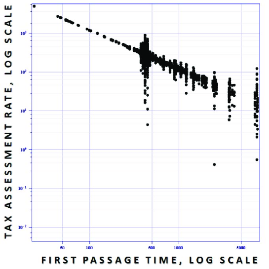
Figure 13: Tax assessment rate (TAR) of places in Manhattan (the vertical axes, in $/fit²) is shown in the logarithmic scale vs. the first–passage times (FPT) to them (the horizontal axes).

The current tax assessment system enacted in 1981 in the city of New York classifies all real estate parcels into four classes subjected to the different tax rates set by the legislature: (i) primarily residential condominiums; (ii) other residential property; (iii) real estate of utility corporations and special franchise properties; (iv) all other properties, such as stores, warehouses, hotels, etc. However, the scarcity of physical space in the compact urban pattern on the island of Manhattan will naturally set some increase of value on all desirably located land as being a restricted commodity. Furthermore, regulatory constraints on housing supply exerted on housing prices by the state and the city in the form of ’zoning taxes’ are responsible for converting the property tax system in a complicated mess of interlocking influences and for much of the high cost of housing in Manhattan, Glaeser:2003 .

Being intrigued with the likeness of the tax assessment map and the map of isolation in Manhattan, we have mapped the TAR figures publicly available through the Office of the Surveyor at the Manhattan Business Center onto the data on first-passage times to the corresponding places. The resulting plot is shown in Fig. 13, in the logarithmic scale. The data presented in Fig. 13 positively relates the geographic accessibility of places in Manhattan with their ’unearned increments’ estimated by means of the increasing burden of taxation. The inverse linear pattern dominating the data is best fitted by the simple hyperbolic relation between the tax assessment rate (TAR) and the value of first–passage time (FPT), $\mathrm{TAR}\approx{c}/{\mathrm{FPT}},$ in which $c\simeq 120,000\$\times\mathrm{Step}/\mathrm{fit}^{2}$ is a fitting constant.

7 First attaining times manifold. The Morse theory

In Sec. 3, we have shown that each node of a finite connected undirected graph, or a relational database can be described by a vector in the projective $(N-1)-$dimensional space, with the (squared) norm of the vector interpreted as the first-passage time to the node by the random walks, starting from the stationary distribution. We have shown that the first-passage time can be calculated as the mean of all first hitting times, $f_{j}=\sum_{i\geq 1}\pi_{i}H_{ij},$ with respect to the stationary distribution of random walks $\pi=\psi_{1}^{2}.$ For any given starting distribution $\phi_{1}^{2}$ that differs from the stationary one, we can also calculate the analogous quantity,

$$\tilde{f}_{j}\left(\phi_{1}\right)\,\,=\,\,\sum_{i=1}^{N}\phi_{1,i}^{2}H_{i,j},$$ (24)

which we call the first attaining time to the node $j$ by the random walks starting at the distribution $\phi_{1}.$ In the present section, we demonstrate that first attaining times of a finite undirected connected graph form a manifold (the first attaining times manifold) in the $(N-1)-$dimensional probabilistic space, for which the first-passage times $f_{j}$ calculated with respect to the stationary distribution of random walks play the role of critical values. Below, we analyze the topology of the first attaining times manifolds by calculating their Euler characteristic and show that these manifold might have a fiber topological structure.

Let us consider the random walks starting from a distribution different from the stationary one,

$$\phi_{1}\,\,=\,\,\left(1-\sum_{\kappa=2}^{N}\varepsilon_{\kappa}\right)\psi_{1}+\sum_{\kappa=2}^{N}\varepsilon_{\kappa}\psi_{\kappa},$$ (25)

in which $\varepsilon_{\kappa}>0$ is the magnitude of deviation of the vector $\phi_{1}$ from $\psi_{1}$ in the direction $\kappa$. From the natural normalization condition for distributions,

$$1\,\,=\,\,\sum_{i=1}^{N}\phi_{1,i}^{2}\,\,=\,\,\sum_{i=1}^{N}\left(\left(1-\sum_{\kappa=2}^{N}\varepsilon_{\kappa}\right)\psi_{1,i}+\sum_{\kappa=2}^{N}\varepsilon_{\kappa}\psi_{\kappa,i}\right)^{2},$$

it follows that

$$\left(1-\sum_{\kappa=2}^{N}\varepsilon_{\kappa}\right)^{2}\,\,=\,\,1-\sum_{\kappa=2}^{N}\varepsilon^{2}_{\nu},\quad|\varepsilon_{\kappa}|<1.$$ (26)

Then, the first attaining time for the node $j$ by the random walks starting from the distribution $\phi_{1}$ is given by

$$\begin{array}[]{ll}\tilde{f}_{j}\,\,=\,\,\sum_{i=1}^{N}\phi_{1,i}^{2}H_{i,j}&=f_{j}\cdot\left(1-\sum_{\kappa=2}^{N}\varepsilon_{\kappa}\right)^{2}\\ &+{\sum_{i=1}^{N}\left(2\left(1-\sum_{r=2}^{N}\varepsilon_{r}\right)\sum_{\kappa=2}^{N}\varepsilon_{\kappa}\psi_{1,i}\psi_{\kappa,i}\sum_{s=2}^{N}\frac{1}{\lambda_{s}}\left(\frac{\psi_{s,j}^{2}}{\psi_{1,j}^{2}}-\frac{\psi_{s,j}}{\psi_{1,j}}\frac{\psi_{s,i}}{\psi_{1,i}}\right)\right)}\\ &+\sum_{i=1}^{N}\left(\sum_{\kappa=2}^{N}\varepsilon_{\kappa}\psi_{\kappa,i}\right)^{2}\sum_{s=2}^{N}\frac{1}{\lambda_{s}}\left(\frac{\psi_{s,j}^{2}}{\psi_{1,j}^{2}}-\frac{\psi_{s,j}}{\psi_{1,j}}\frac{\psi_{s,i}}{\psi_{1,i}}\right).\end{array}$$ (27)

Taking into account the orthogonality condition for the eigenvectors $\psi_{k}$ and the relation (26), we further obtain,

$$\begin{array}[]{ll}\tilde{f}_{j}&{\,\,=\,\,f_{j}\cdot\left(1-\sum_{\kappa=2}^{N}\varepsilon_{\kappa}\right)^{2}+f_{j}\cdot\sum_{i=1}^{N}\left(\sum_{\kappa=2}^{N}\varepsilon_{\kappa}\psi_{\kappa,i}\right)^{2}-\sum_{i=1}^{N}\left(\sum_{\kappa=2}^{N}\varepsilon_{\kappa}\psi_{\kappa,i}\right)^{2}\sum_{s=2}^{N}\frac{1}{\lambda_{s}}\frac{\psi_{s,j}}{\psi_{1,j}}\frac{\psi_{s,i}}{\psi_{1,i}}}\\ &{\,\,=\,\,f_{j}\cdot\left(1-\sum_{\kappa=2}^{N}\varepsilon_{\kappa}\right)^{2}+f_{j}\cdot\left(2\sum_{\kappa,\nu=2}^{N}\left(1-\delta_{\kappa\nu}\right)\varepsilon_{\kappa}\varepsilon_{\nu}\underbrace{\sum_{i=1}^{N}\psi_{\kappa,i}\psi_{\nu,i}}_{0}+\sum_{\nu=2}^{N}\varepsilon_{\nu}^{2}\underbrace{\sum_{i=1}^{N}\psi_{s,i}^{2}}_{1}\right)-}\\ &{\,\,\,\,-\sum_{i=1}^{N}\left(2\sum_{\kappa,\nu=2}^{N}\left(1-\delta_{\kappa\nu}\right)\varepsilon_{\kappa}\varepsilon_{\nu}\psi_{\kappa,i}\psi_{\nu,i}\sum_{s=2}^{N}\frac{1}{\lambda_{s}}\frac{\psi_{s,j}}{\psi_{1,j}}\frac{\psi_{s,i}}{\psi_{1,i}}+\sum_{s=2}^{N}\varepsilon_{s}^{2}\psi_{s,i}^{2}\sum_{l=2}^{N}\frac{1}{\lambda_{l}}\frac{\psi_{l,j}}{\psi_{1,j}}\frac{\psi_{l,i}}{\psi_{1,i}}\right)}\\ &{\,\,=\,\,f_{j}\cdot\underbrace{\left(\left(1-\sum_{\kappa=2}^{N}\varepsilon_{\kappa}\right)^{2}+\sum_{\nu=2}^{N}\varepsilon_{\nu}^{2}\right)}_{1}-2\cdot\sum_{\kappa,\nu=2}^{N}\varepsilon_{\kappa}\varepsilon_{\nu}\sum_{s=2}^{N}\frac{1}{\lambda_{s}}\frac{\psi_{s,j}}{\psi_{1,j}}\sum_{i=1}^{N}\frac{\left(1-\delta_{\kappa\nu}\right)\psi_{\kappa,i}\psi_{\nu,i}\psi_{s,i}}{\psi_{1,i}}}\\ &{{\rm\;\;\;}-\delta_{\kappa\nu}\sum_{\kappa=2}^{N}\varepsilon_{\kappa}^{2}\sum_{s=2}^{N}\frac{1}{\lambda_{s}}\frac{\psi_{s,j}}{\psi_{1,j}}\sum_{i=1}^{N}\frac{\psi_{\kappa,i}^{2}\psi_{s,i}}{\psi_{1,i}}.}\end{array}$$

Below, we introduce the following notations for the vectors in the $(N-1)-$dimensional projective space $P\mathbb{R}^{(N-1)}$,

$${\Omega}^{\kappa,\nu}\,\,=\,\,\left\{\frac{1}{\sqrt{\lambda_{s}}}\sum_{i=1}^{N}\frac{\psi_{\kappa,i}\psi_{\nu,i}\psi_{s,i}}{\psi_{1,i}}\right\}_{s=2}^{N},\quad{\bf q}_{i}\,\,=\,\,\left\{\frac{1}{\sqrt{\lambda_{s}}}\frac{\psi_{s,i}}{\psi_{1,i}}\right\}_{s=2}^{N}\,\,\in\,\,P\mathbb{R}^{(N-1)},$$ (28)

and obtain the following expression for the first attaining times,

$$\tilde{f}_{j}\,\,=\,\,{f}_{j}-\sum_{\kappa,\nu=2}^{N}\varepsilon_{\kappa}\varepsilon_{\nu}\left({\bf q}_{j},\Omega^{\kappa,\nu}\right)_{P\mathbb{R}^{(N-1)}}\,\,=\,\,\left({\bf q}_{j},{\bf q}_{j}-\sum_{\kappa,\nu=2}^{N}\varepsilon_{\kappa}\varepsilon_{\nu}\Omega^{\kappa,\nu}\right)_{P\mathbb{R}^{(N-1)}}$$ (29)

where $(\bullet,\bullet)_{P\mathbb{R}^{(N-1)}}$ denotes the usual scalar product in $P\mathbb{R}^{(N-1)}.$ The second order derivative of the first attaining time in the directions $\kappa,\nu$ (i.e., the Hessian function) is a symmetric matrix for any node $j$,

$${\mathcal{H}}_{\kappa\nu}(j)\,\,\equiv\,\,\frac{\partial^{2}\tilde{f}_{j}}{\partial\varepsilon_{\kappa}\partial\varepsilon_{\nu}}\,\,=\,\,-\left({\bf q}_{j},\Omega^{\kappa,\nu}\right)_{P\mathbb{R}^{(N-1)}}\,\,=\,\,{\mathcal{H}}_{\nu\kappa}(j).$$ (30)

Therefore, in a neighborhood of every node $j$, the first attaining time $\tilde{f}_{j}$ can be expressed as

$$\tilde{f}_{j}\,\,=\,\,{f}_{j}+\left({\bf q}_{j},\left(\sum_{\kappa,\nu=2}^{N}\varepsilon_{\kappa}\varepsilon_{\nu}\frac{{\mathcal{H}}_{\kappa\nu}(j)}{\|{\bf q}_{j}\|_{T}}\right)\,{\bf q}_{j}\right)_{P\mathbb{R}^{(N-1)}}.$$ (31)

where the first-passage time $f_{j}=\left({\bf q}_{j},{\bf q}_{j}\right)_{P\mathbb{R}^{(N-1)}}$, explicitly establishing the homeomorphism to the Euclidean space of dimension $(N-1).$ We conclude that the first attaining times of all nodes of a finite connected undirected graph form a manifold with respect to possible starting distributions of the random walks. It is important to mention that the gradients of the first attaining times to any node $j$ uniformly equal zero at the vicinity of the stationary distribution,

$$\nabla_{\kappa}\tilde{f}_{j}\equiv\left.\frac{\partial\tilde{f}_{j}}{\partial{\varepsilon}_{\kappa}}\right|_{\varepsilon_{\nu}=0}\,\,=\,\,\left.-\sum_{\nu=2}^{N}\varepsilon_{\nu}\left({\bf q}_{j},\Omega^{\kappa,\nu}\right)_{P\mathbb{R}^{(N-1)}}\right|_{\varepsilon_{\nu}=0}\,\,=\,\,0.$$ (32)

Therefore, each node $j$ is a critical point of the manifold of first attaining times, and the first passage times $f_{j}$ are the correspondent critical values. Furthermore, following the ideas of the Morse theory Matsumoto:2002 , we can perform the standard classification of the critical points, saying that a critical point $j$ is non-degenerate if the Hessian matrix (30) is non-singular at $j$ and introducing the index $\gamma_{j}$ of the non-degenerate critical point $j$ as the number of negative eigenvalues of (30) at $j$ (i.e., the dimension of the largest subspace of the tangent space to the manifold at $j$ on which the Hessian is negative definite).

The Euler characteristic $\chi$ is an intrinsic property of a manifold that describes its topological space’s shape regardless of the way it is bent. It is known that the Euler characteristic can be calculated as the alternating sum of $C^{\gamma},$ the numbers of critical points of index $\gamma$ of the Hessian function,

$$\chi\,\,=\,\,\sum_{\gamma\geq 0}(-1)^{\gamma}C^{\gamma}.$$ (33)

In Fig. 14, we have presented the Euler characteristics for the first attaining times manifolds calculated for the webs of city canals in Amsterdam (57 canals) and Venice (96 canals).

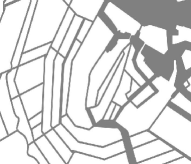
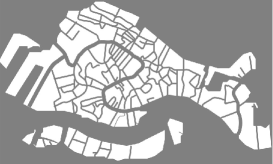
$\chi=-5$	$\chi=4$

Figure 14: The Euler characteristics for the first attaining times manifolds calculated for the webs of city canals in Amsterdam (57 canals) and Venice (96 canals).

It is interesting to note that the functions of the canal networks created in Venice and in Amsterdam were historically different. While the Venetian canals mostly serve the function of transportation routes between the distinct districts of the gradually growing naval capital of the Mediterranean region, the concentric web of Amsterdam gratchen had been built in order to defend the city. The central diamond within a walled city was thought to be a good design for defense. Many Dutch cities have been structured this way: a central square surrounded by concentric canals. The city of Amsterdam is located on the banks of the rivers Amstel and Schinkel, and the bay IJ. It was founded in the late 12th Century as a small fishing village, but the concentric canals were largely built during the Dutch Golden Age, in the 17th Century. The principal canals are three similar waterways, with their ends resting on the IJ, extending in the form of crescents nearly parallel to each other and to the outer canal. Each of these canals marks the line of the city walls at different periods. Lesser canals intersect the others along the radial direction, dividing the city into a number of islands. The resulting structure is highly symmetric, and the Euler characteristic of the corresponding first attaining times manifold is negative ($\chi=-5$). It is known that the negative Euler characteristics could either come from a pattern of symmetry in the hyperbolic surfaces, or from a manifold homeomorphic multiple tori.

In contrast to the highly symmetric and planned structure of the canal network in Amsterdam, the network of Venetian canals was developed gradually, in a long historical process of urban development started from the 6th Century, at the oldest settlements in Venice that had appeared in Dorsoduro, along the Giudecca Canal. By the 11th Century, settlement had spread to the Grand Canal. The Giudecca island was composed of eight islets separated by canals dredged in the 9th Century when the area was divided among the rebelling nobles. The primary traditional divisions of Venice into sestieri (Cannaregio, San Polo, Dorsoduro, Santa Croce, San Marco and Castello, Giudecca) was developed from the early Middle Ages to the 20th Century. The Euler characteristic of the first attaining times manifold corresponding to the resulting network of Venetian canals is $\chi=4$. The large positive value of the Euler characteristic can arise due to the well-known product property of Euler characteristics $\chi(M\times N)=\chi(M)\cdot\chi(N)$, for any product space $M\times N,$ or, more generally, from a fibration, when one topological space (called a fiber) is being ”parameterized” by another topological space (called a base).

8 Discussion and Conclusion

In the present paper, in order to geometrize and interpret the data, we propose the use of a path integral distance, in which all possible paths between any two nodes in a graph model of the data are taken into account, although some paths are more preferable than others. We have pointed out that the process of data interpretation is always based on the implicit introduction of certain equivalence relations on the set of walks over the database. It is clear that different equivalence relations might lead to the different concepts of taxonomic categories and generate the different concept for representing the data. Therefore, an interpretation process does not necessary reveal a ”true meaning” of the data, but rather represents a self-consistent point of view on that.

Given a probability measure on the set of all walks in the graph model of the database, every equivalence relation defines the discrete time random walks of a certain scale, in which all equivalent walks are equiprobable. We have shown that the random walks of different scales are dramatically dissimilar: while the nearest-neighbor random walks homogeneously cover the whole available space within the given environment, the high scale random walks are obstacle repelling, as the centrality measure (quantifying the fraction of paths of the length $n>1$ traversing the node) is sensitive to defects and dramatically decreases in the vicinity of obstacles and boundaries. As the scale of the random walk increases, the level of transition randomness quantified by the entropy rate shows almost the logarithmic growth, approaching its maximum for the maximum entropy random walks $T^{(\infty)}.$ At the same time, the behavior of the excess entropy (”complexity”, ”the past-future mutual information”) is complementary, decreasing from its maximal value attained for the nearest-neighbor random walks to the walks characterized by the minimal dependence on the past path attained for the maximum entropy random walks $T^{(\infty)}.$ In order to study the relation between the order of transitions and the structural correlations within an environment by the complexity -entropy relations in the three different environments of increasing structural complexity. We have shown that the relation between structure and order in the random transitions within an ”empty room” is straightforward across the different scales: the structure provided merely by the walls, bounding the environment reinforces the order. As the number of obstacles within the environment increases, such the reinforcement becomes even more visible, especially for the large scale random walks. As the structural complexity of the environment further increases, the phenomenon of localization of random walkers inside the spaces formed by the filamentary sequences of the closely located obstacles comes into play at the short-range random walks $T^{(2)}.$

The random walks allow us to geometrize the data by introducing the new graph distance, in which all possible paths between any two nodes are taken into account. The idea of the path integral generalizes the action principle of classical mechanics replacing a single trajectory of a particle with a sum over all possible trajectories to compute the probability amplitude (propagator). The path integral calculation can be viewed as the left inverse of the Laplace operator describing the diffusion process of particles. The inverse of the Laplace operator describing the spread of particles in an environment is not unique, however we can choose such the generalized inverse of it which share the same set of symmetries as the Laplace operator itself (the Drazin generalized inverse). It is important to mention that the calculation of the Green’s function for the diffusion process give rise to a non-trivial geometric framework for description of graphs and relational databases. In particular, each node of the finite connected undirected graphs can be described by a vector in the projective $(N-1)-$dimensional space, with the squared norm of the vector interpreted as the first-passage time to the node by the random walks, starting from the stationary distribution. The image of the graph in such the probabilistic projective space constitutes a diffusion manifold of self-avoiding random walks in affine space, as we can subtract the graph nodes (by component wise subtracting of their images) to get vectors, or add vectors to a vertex to get another vertex, but we cannot add new vertices. In our paper, we consider some examples of the use of the probabilistic geometry for the description of structural properties of mazes, musical compositions, and the various urban neighborhoods. We have found that the relation between the recurrence time and the first -passage time to the node can play the crucial role for the interpretation of its role within the structure. Namely, the isolated places for which the first-passage times are longer than the recurrence times to them might be interpreted as obscure, since the walker appears to be trapped within them. On the contrary, the nodes characterized with the first-passage times shorter than the recurrence time can play the important role, providing the guide to the environment and increasing its intelligibility. One fascinating example is the tonality structure in the western musical compositions.

Being interested in the interpretation of urban spatial patterns, we have analyzed the first-passage times in the canal network of Venice and the urban pattern on Manhattan. The first -passage times enable us to classify all places of movement in the urban spatial graph accordingly to their statistical isolations. It is remarkable that the obtained classification of places correspond to the spatial distribution of the tax assessment rate of sites that relies upon a special enhancement made up of the site value.

Finally, we consider the quantity similar to the first- passage times, which we have called the first attaining times, quantifying the first -passage time to the node by the random walk starting from a distribution that differs from the stationary one. We have shown that the set of the first attaining times form a manifold within the projective probabilistic space, for which the first-passage times plays the role of critical values. The Euler characteristics of the studied real-world graphs (canal networks in Venice and Amsterdam) show that these manifold might have a fiber topological structure.

References

- (1) SINTEF (2013, May 22). ”Big Data, for better or worse: 90% of world’s data generated over last two years”. ScienceDaily. Retrieved December 17, 2013, from http://www.sciencedaily.com/releases/2013/05/130522085217.htm.
- (2) Volchenkov, D., ”Markov Chain Scaffolding of Real World Data”, Discontinuity, Nonlinearity, and Complexity 2(3) 289-299 (2013)— DOI: 10.5890/DNC.2013.08.005.
- (3) Graham, A., 1987. Nonnegative Matrices and Applicable Topics in Linear Algebra, John Wiley & Sons, New York.
- (4) J.P. Crutchfield, N.H. Packard, Symbolic dynamics of noisy chaos, Physica D: Nonlinear Phenomena 7(1-3), 201-223 (1983).
- (5) R. Shaw, The dripping faucet as a model chaotic system, CA Aerial Press, Santa Cruz (1984).
- (6) W. Li, ”On the relationship Between Complexity and Entropy for Markov Chains and Regular Languages”, Complex systems 5, 381 (1991).
- (7) Feldman, D.P., McTague, C.S., Crutchfield, J.P., ”The organization of intrinsic computation: Complexity-entropy diagrams and the diversity of natural information processing”, Chaos 18, 043106 (2008).
- (8) Fan Chung, S.-T. Yau, ”Discrete Green’s functions”, Journal of Combinatorial Theory (A) 91, 191-214 (2000).
- (9) Blanchard,Ph., Volchenkov, D., Introduction to Random Walks on Graphs and Databases, Springer Series in Synergetics , Vol. 10, Berlin / Heidelberg, ISBN 978-3-642-19591-4 (2011).
- (10) Chung, F.R.K., 1997. Lecture notes on spectral graph theory, AMS Publications Providence.
- (11) Lovász, L., 1993. ”Random Walks On Graphs: A Survey.” Bolyai Society Mathematical Studies 2: Combinatorics, Paul Erdös is Eighty, 1, Keszthely (Hungary).
- (12) D. Coppersmith, P. Tetali, P. Winkler. ”Collisions among random walks on a graph”. SIAM J. on Discrete Math. 6(3), 363 (1993).
- (13) H. Kern, ”VIII. Church Labyrinths”. Through the Labyrinth: Designs and Meaning Over 5,000 Years. Prestel. ISBN 978-3-7913-2144-8 (2000).
- (14) C. Schuster, E. Carpenter, Patterns that Connect: Social Symbolism in Ancient & Tribal Art. Harry N. Abrams. Pub. p. 307. ISBN 978-0-8109-6326-9 (1996).
- (15) M. Kac, ”On the Notion of Recurrence in Discrete Stochastic Processes”, Bull. Am. Math. Soc. 53, 1002 (1947) [Reprinted in M. Kac Probability, Number Theory, and Statistical Physics: Selected Papers, K. Baclawski, M.D. Donsker (eds.), Cambridge, Mass.: MIT Press, Series: Mathematicians of our time Vol. 14, 231 (1979)].
- (16) Erdélyi,I., 1967. ”On the matrix equation .” J. Math. Anal. Appl. 17, 119.
- (17) Meyer, C.D., 1975. ”The role of the group generalized inverse in the theory of finite Markov chains”, SIAM Rev. 17, 443.
- (18) Drazin, M.P., 1958. ”Pseudo-inverses in associative rings and semigroups”. The American Mathematical Monthly 65, 506.
- (19) Ben-Israel, A., Greville, Th.N.E., 2003. Generalized inverses: theory and applications. Springer; 2nd edition.
- (20) Muir, T., 1960. Treatise on the Theory of Determinants (revised and enlarged by W. H. Metzler), Dover, New York.
- (21) Robert, P., 1968. ”On the group inverse of a linear transformation”, J. Math. Anal. Appl. 22, 658.
- (22) Campbell, S.L., Meyer, C.D., Rose, N.J., 1976. ”Applications of the Drazin Inverse to Linear Systems of Differential Equations with Singular Constant Coefficients”, SIAM J. Appl. Math. 31(3), 411.
- (23) Hartwig, R.E., 1976. ”More on the Souriau-Frame Algorithm and the Drazin Inverse”, SIAM J. Appl. Math. 31 (1), 42.
- (24) Agaev, R.P., Chebotarev, P.Yu., 2002. ”On Determining the Eigenprojection and Components of a Matrix”, Automation and Remote Control 63 (10), 1537.
- (25) H. Noguchi, ”Mozart: Musical game in C K.516f”. Available at http://www.asahi-net.or.jp/ rb5h-ngc/e/k516f.htm (1996).
- (26) C Dahlhaus, ”Harmony”. Grove Music Online, ed. L. Macy at www.grovemusic.com (2007).
- (27) W. Thomson, Tonality in Music: A General Theory., San Marino, Calif.: Everett Books (1999).
- (28) E.M. Burns, Intervals, Scales, and Tuning. The Psychology of Music. Second edition, Deutsch, Diana, ed. San Diego: Academic Press (1999).
- (29) B. Hillier, J. Hanson, The Social Logic of Space (1993, reprint, paperback edition ed.). Cambridge: Cambridge University Press (1984).
- (30) B. Jiang, C. Claramunt, Topological analysis of urban street networks. Environment and Planning B: Planning and Design 31, 151, Pion Ltd. (2004).
- (31) L. Wirth, The Ghetto (edition 1988) Studies in Ethnicity; Transaction Publishers, New Brunswick (USA), London (UK) (1928).
- (32) L. Vaughan, ”The relationship between physical segregation and social marginalization in the urban environment.” World Architecture, 185, 88 (2005).
- (33) L. Vaughan, D. Chatford & O. Sahbaz Space and Exclusion: The Relationship between physical segregation. economic marginalization and poverty in the city, Paper presented to Fifth Intern. Space Syntax Symposium, Delft, Holland (2005).
- (34) D. Volchenkov, Ph. Blanchard, ”Random Walks Along the Streets and Channels in Compact Cities : Spectral analysis, Dynamical Modularity, Information, and Statistical Mechanics”, Phys. Rev. E 75, 026104 (2007).
- (35) D. Volchenkov, Ph. Blanchard, Scaling and Universality in City Space Syntax: between Zipf and Matthew. Physica A 387(10), 2353 ( 2008), doi:10.1016/j.physa.2007.11.049.
- (36) Ph. Blanchard, D. Volchenkov, Mathematical Analysis of Urban Spatial Networks, Springer Series Understanding Complex Systems, Berlin / Heidelberg. ISBN 978-3-540-87828-5, 181 pages (2009).
- (37) B. Hillier, The common language of space: a way of looking at the social, economic and environmental functioning of cities on a common basis, Bartlett School of Graduate Studies, London (2004).
- (38) R.P. Bolton, Building For Profit. Reginald Pelham Bolton (1922).
- (39) E.L. Glaeser, J. Gyourko, Why is Manhattan So Expensive? Manhattan Institute for Policy Research, Civic Report 39 (2003).
- (40) Y. Matsumoto, An Introduction to Morse Theory. In Iwanami Series in Modern Mathematics, American Mathematical Soc., ISBN-13: 978-0-8218-1022-4 (2002).