Linear response of hydrodynamically-coupled particles under a nonequilibrium reservoir
Abstract
A recent experiment driving colloids electromagnetically, by Bérut et al. [1], is an ideal paradigm for illustrating a linear response theory for nonequilibrium overdamped systems including hydrodynamic interactions and, unusually, a reservoir itself out of equilibrium. Indeed, in this setup one finds a nonequilibrium environment in which the mobility and diffusivity of free particles are not simply proportional to each other. We derive both the response to a mechanical forcing and to temperature variations in terms of correlations between an observable and a path-weight action. The time-antisymmetric component of the latter turns out not to be simply proportional to the heat flowing into the environment. These results are visualized with simulations resembling conditions and protocols easily realizable in the experiment, thereby tracing a path for experimental verifications of the theory.
pacs:
05.40.-a,05.70.LnKeywords: Nonequilibrium statistical mechanics, fluctuation-response relations, hydrodynamic interactions.
1 Introduction
Objects immersed in a fluid feel the presence of each other from a distance via mediation of the fluid itself. This hydrodynamic interaction is usually much faster than the rearrangements of the objects so that it appears to be a long-range instantaneous effect, as those usually modeled with energy potentials [2].
There are hydrodynamic systems that are becoming a new paradigm of nonequilibrium, such as bacterial motion and driven colloids [3]. In colonies of bacteria one is observing an instance of active matter, where the origin of nonconservative forces is chemically-driven self-propulsion of the single “particles”, and can give rise to complex phase behaviour [4, 5]. On the other hand, colloidal systems constitute more classical examples of systems brought out of equilibrium by external forces. In particular, in the past decade, several experiments of driven colloids were performed with the aim of realizing minimal systems in which new laws of nonequilibrium could be tested [6, 7, 8, 9, 10]. With rotating lasers, a single particle was maintained out of equilibrium by confining it in a toroidal region where an additional rotational drift was imposed [10, 11, 12]. When multiple particles were included in the toroidal region, hydrodynamic effects led to forms of synchronization [13]. Another minimal system was realized recently with two colloids trapped not far from each other, by driving the first particle with a rapidly varying random electromagnetic field [1], which thus played the role of an additional component to the heat bath. The temperature of this particle effectively increased by this driving and the influence was transmitted to the second particle thanks to hydrodynamic interaction. We will use this experiment as our guideline to introduce a theory for the linear response of overdamped nonequilibrium systems, with hydrodynamic coupling and subject to a heat bath that includes a nonequilibrium component.
Knowing how a system responds to small perturbations is at the basis of linear response. In equilibrium there is a celebrated result, the fluctuation-dissipation theorem [14], which states that measuring the correlations between an observable and a specific potential in the unperturbed equilibrium regime is sufficient for predicting how the observable would react to the addition of a tiny amount of such energetic potential. In the same fashion, responses to a change in the bath temperature of a system in thermodynamic equilibrium may be related to unperturbed correlations [14]. Both scenarios are actually expressions of a general relation, known as Kubo formula. It has thus been stressed (e.g., [15, 16]) that to predict the response in equilibrium, the only relevant quantity is the entropy that the perturbing entity would produce in the dissipation toward a new equilibrium.
There are several approaches trying to generalize the fluctuation-dissipation theory to nonequilibrium conditions, see references in [17, 16]. In some cases the knowledge of the microscopic density of states is required [18, 19, 20]. In other approaches there emerges the need to understand not only entropy, which is antisymmetric with respect to time-reversal, but also other time-symmetric dynamical aspects [21, 22, 15]. The latter is not related to dissipation but rather to the “activation” of the dynamics by means of the perturbation. In fact, a perturbation may not only lead to an increased or decreased tendency to dissipate but additionally to a modified “frenesy” [15, 23, 24, 16, 25] of the system. Such frenesy quantifies how a perturbation changes the mean propensity of the system to escape from a neighborhood in state space. For instance, in the case of discrete systems, the frenesy indicates how the mean tendency to jump from state to state is modified by a perturbation. Specifically, in a given trajectory it is not proportional to the actual number of jumps, that is, to the actual dynamical activity [26, 27, 28], but it is rather an estimator of the escape rate (a kind of “wished” activity) integrated in time.
Within the scope of nonequilibrium statistical physics, one usually considers a system driven out of equilibrium by a nonconservative force, or one where degrees of freedom interact with baths under different equilibrium conditions. Multiple heat baths as in the latter situation are generally employed in the study of heat transfer between equilibrium baths at different temperatures, mediated by mechanically-interacting degrees of freedom under their influence [29, 30]. In such models, each degree of freedom is eventually thermalized by a separate equilibrium reservoir. The experimental situation briefly mentioned above [1] also exhibits a nonequilibrium maintained by a thermal reservoir with different effects on different degrees of freedom, this time introduced by the additional noise. However, the hydrodynamic coupling present puts a twist on the scenario. Now, the particles receive (and dissipate) energy from (and to) the reservoir via one another as well as directly. Therefore the action of the additional thermal component cannot be decoupled from the fluid’s, and the exchanges with the reservoir cannot be placed in the framework of equilibrium thermodynamics even from the point of view of the reservoir. However, this simple system serves as a model where the nonequilibrium, or loss of detailed balance, in the reservoir is quantifiable, as discussed in the following section.
In the present article, we develop the linear response theory for a system of hydrodynamically coupled degrees of freedom where thermal equilibrium in the reservoir is broken, in the sense described in the previous paragraph, by the presence of additional components. From the point of view of Langevin dynamics, this amounts to a diffusivity that is not proportional to the mobility, as local detailed balance would have required. We discuss first the case of perturbing the mechanical forces, generalizing, in the necessary fashion, a fluctuation-response relation based on path probabilities [15, 23]. In the colloidal model system we consider, manipulation of the artificial temperature is also an easy and natural operation. Therefore, we deal also with fluctuation response relations for temperature variations, further generalizing a recent analysis of temperature response [31]. In both of these cases, be it a perturbation of the deterministic influences or the thermal ones, we see signatures of the particular out of equilibrium condition and especially the nonvanishing correlation between the degrees of freedom due to hydrodynamic coupling. We illustrate our findings by data from numerical experiments.
Furthermore, from considering path probabilities, the nonequilibrium situation maintained by the non-proportionality between diffusivity and mobility hint at possible caveats on identifying the time-antisymmetric part of the path action with dissipated heat. Indeed, the relationship between dissipated heat and entropy is a temperature, which is not possible to identify unequivocally by simply looking at the reservoir, since the reservoir is not made up of separate heat baths at well-defined temperatures. Within the distinct framework of the experimental paradigm of Ref. [1], it is possible to write an explicit expression for the dissipation, upon which we see that it contains terms that are not of the form of heat in the sense of stochastic thermodynamics, but those that couple the forces and displacements across different particles. This seems to be a form of housekeeping entropy [32, 33, 34], incurred by the breaking of detailed balance by the artificial temperature on one particle.
The article is organized as follows: Sec. 2 establishes the Langevin dynamics framework within which we address the problem. Here, we show explicitly how the artificial noise is encoded in the diffusivity matrix, and proceed with a concise review of the experimental paradigm along with its placement into the framework. Sec. 3 begins with a review of the path integral framework in the context of linear response, and moves on to explicit expressions for the particular physical situation under consideration. From this perspective, the aforementioned peculiarities of heat and entropy production are discussed. In Sec. 4, we derive the linear response formula for deterministic perturbations and apply it to a situation where optical trap strengths are manipulated. The section ends with results and discussion of numerical experiments measuring the associated susceptibility of the energies stored in the traps. Similarly, in Sec. 5 we discuss the linear response to variations of the artificial temperature and provide results of illustrative numerical experiments, before we conclude the article.
2 Stochastic framework
Let us begin with a concise discussion on the stochastic dynamics of the type of systems investigated in this article, and establish aspects of notation. First we explain how hydrodynamic coupling and the presence of an additional (electromagnetic) random forcing should be incorporated. Afterwards, we specialize these arguments to the particular experimental situation that serves as the central physical paradigm for the scope of this article.
2.1 Langevin dynamics
The degrees of freedom describing the system are the coordinates of micrometer-sized particles in an aqueous solvent. At this scale, inertia becomes irrelevant; momenta are excluded and the dynamics is overdamped. Therefore, the dynamics will be determined by a system of coupled overdamped Langevin equations, such as
| (1) |
where time dependences of and have been omitted for brevity of notation, and Einstein’s summation convention is understood.111On occasion, we will use matrix notation instead of indices. In these instances we will use boldface symbols in place of collections of numbers, be it vectors (as in the argument of ) or matrices. The vector of colorless Gaussian differential noises has uncorrelated components, i.e., . Any correlations in the random forcing, therefore, are captured in the (force-free) diffusion matrix , which is symmetric.222The expression stands for a matrix which satisfies . As such, the matrix is not unique; there is freedom to choose with an orthogonal transformation, without affecting the physical content [35]. The symmetric (free-particle) mobility matrix embodies inverse drag coefficients originating from the dissipative nature of the fluid, and is the deterministic force on the degree of freedom . The mobility and diffusion coefficients are assumed to be state-independent. This is an approximation that is suitable for the particular physical paradigm we focus on, as explained later in Sec. 2.3.
2.2 A multicomponent bath with hydrodynamic coupling
Hydrodynamic coupling implies that forces on one degree of freedom affect the motion of other degrees of freedom via propagation through the fluid. Hence, the mobility matrix is not diagonal. Since the same applies to the random forces exerted by the fluid, the random forcing term also embodies correlation between different degrees of freedom, encoded in the off-diagonal elements of the diffusivity matrix .
In this article, we deal with an aqueous environment at a temperature . The dissipative and fluctuating effects of the fluid, namely the damping of motion (encoded in ) and the stochastic energy pumping (encoded in ), balance each other. This is formalized by the so-called second fluctuation-dissipation theorem [14, 17] (with Boltzmann’s constant set to ) as,
| (2) |
However, the aqueous environment is considered as just one component of a larger, “multicomponent” bath. This is inspired by recent experiments [1] where colloids were placed in solution via optical tweezers subjected to random oscillations, effectively thermalizing the particles at different temperatures. A conceptual description where the bath consists of aqueous and electromagnetic components suits this system. In such a case with multiple thermalizing influences, the proportionality (2) between mobility and diffusion is broken. One can separate the diffusion matrix into separate contributions from the fluid and the electromagnetic field.
The aforementioned random oscillation of the optical traps was generated through white noise, and hence enters the dynamics of the system as a stochastic force in addition to that of the aqueous environment. In other words, we have
| (3) |
appropriately labeling the parts due to the aqueous environment and the electromagnetic field of the optical traps. One can write a completely equivalent equation,
| (4) |
by adding the diffusion (or covariance) matrices, as a result of the fact that the sum of two independent Gaussian random variables is still a Gaussian random variable whose variance is the sum of the two original variances. Hence, the multicomponent reservoir is described by a diffusion matrix
| (5) |
Underlying this additive separation of diffusion matrices (5), or of stochastic forces (3), there is one assumption: Despite the influence of the electromagnetic components, the aqueous bath remains in equilibrium at temperature , still satisfying the fluctuation relation (2). This assumption was also adhered to in the analysis of Ref. [1], where agreement with experimental measurements was demonstrated using (cross-)correlations of the coordinates in a steady state.
The remaining question is the form of the diffusion matrix . In practice, it is not the components of that are under direct experimental control, but the artificial random force, , that is acting on each degree of freedom . More specifically, the experimenter knows the correlation function,
| (6) |
of the colorless Gaussian random forcing. For instance, each component might be statistically independent leading to a diagonal correlation matrix , or all but one might vanish leading to a projector-like matrix, the latter being the specific case realized in the experiment of Ref. [1]. It is then straightforward to relate the diffusion matrix to the correlation matrix by simply noting that according to the equation of motion (3), the random force is given as
| (7) |
Requiring this expression to yield the same correlations as Eq. (6) fixes the diffusion matrix to be
| (8) |
Thus, we have described a system where degrees of freedom are subject to overdamped dynamics in a fluid medium in thermal equilibrium, including hydrodynamically mediated correlations, further under the influence of stochastic forces originating from a source separate from the fluid medium. In this fashion, the resulting system is one in contact with a reservoir out of equilibrium due to multiple components. The equation of motion (1) applies to such a system when the diffusion matrix is decomposed as in Eq. (5), which reads
| (9) |
when expressed explicitly in terms of the properties of the fluid and those of the external noise. We note that the arguments above justifying this decomposition do not rely on the coefficients being position-independent, even though we will not be considering that general case.
2.3 Experimental paradigm
A recent experiment [1] is suitably described in the framework laid down above and is chosen to be our central paradigm. A pair of colloids (radius m) were held in narrow optical traps a few microns apart inside water, such that hydrodynamic coupling would not be negligible. The effective stiffness constants () of the optical traps were pN/m, placing the average deviation, , of each coordinate roughly at m, under a typical room temperature pNnm (). Denoting the inter-trap distance by , the smallness of allows an approximation to lowest order in this ratio, leading to two simplifications: (i) The two directions orthogonal to the line joining the traps can be neglected, which lessens the algebraic burden. (ii) The dependence on coordinates of the mobility and diffusion matrices can be ignored, using their values corresponding to the state when each particle is situated at the minimum of their trap (). That is, , and . For the development of the linear response to temperature variations, for the moment it seems particularly challenging to deal with a state-dependent noise prefactor, making this latter simplification useful. This is also in line with the approach taken by the authors of Ref. [1] in their theoretical analysis of the experiment.
Under this approximation, there remain only two degrees of freedom, , and the forces on the particles are described by the (potential) energy function
| (10) |
The energy is divided into two terms, each depending on either or , hence the forces are transmitted between the degrees of freedom only by the fluid, which is captured by the mobility matrix. The mobility matrix corresponding to hydrodynamically coupled identical spherical colloids was discussed, for example, in Refs. [36, 37]. Applied to the case at hand, with two particles moving along the same spatial dimension, we have
| (11) |
where is the drag coefficient for a spherical colloid of radius , and is given as [36, 37]
| (12) |
with the distance between the two colloids. These are the first two terms in a multipole expansion in the ratio , sometimes referred to respectively as Oseen, and Rotne-Prager terms [38]. However, for our purposes, the distinction will not be important.
The crucial ingredient of the experiment of Ref. [1] is the presence of the external stochastic force affecting one coordinate—say coordinate 1—realized through the application of a white noise to the circuitry responsible for positioning the first optical trap. In the framework laid down in the previous section, this amounts to an electromagnetic forcing with a correlation matrix (6) of the form unless . Further identifying an effective temperature (which was called in Ref. [1]) with the power of the noise (see Ref. [39] for further details), one has
| (13) |
In other words, the two thermalizing influences present in the problem can be described by the diffusion matrix (9)
| (14) |
which of course coincides with the analogous coefficient matrix
| (15) |
that was identified from the associated Fokker-Planck equation in Ref. [1].
We will see in further sections of the article that the “inverse temperature matrix” will play a significant role. For reference, let us provide its explicit expression corresponding to this particular situation:
| (16) |
Under equilibrium reservoir conditions (), this is simply equal to . When there is no hydrodynamic coupling (), it is diagonal but with unequal entries, which would correspond to the typical nonequilibrium situation of several decoupled heat baths at unequal (inverse) temperatures.
In the following sections we will investigate the response of a state observable of the system to a small perturbation of either the deterministic or the stochastic (thermal) forces on the degrees of freedom. For instance, a deterministic perturbation () could be realized experimentally with ease by varying the stiffness of the optical traps (). On the other hand, the experimental setup described above also allows the perturbation of the system thermally in a distinct sense: The effective temperature of external noise can in principle be varied virtually as quickly as desired. Therefore, we will investigate the response of the system to small variations of the noise amplitudes encoded in as a result of a variation of the effective temperature, , according to Eq. (14) for instance.
3 Path functionals and fluctuation-response relations
We begin this section by reviewing the path integral framework for linear response, under quite general conditions first, without referring explicitly to hydrodynamic coupling and external noise. This reduces issues of notation and makes the article more self-contained.
3.1 Linear response
The central quantity of interest is the first order change in the expectation value of an observable upon a small perturbation of parameters. Namely, we seek , where is an observable evaluated at time and the symbol for first order variation. The variation of the average arises from the modification of the associated probability weights, which becomes apparent when written as a path integral. Denoting entire trajectories with the symbol ,
| (17) |
where is the probability measure in the vicinity of in trajectory space. Reserving an explicit expression for the path probability for a subsequent subsection, the variation of the expectation value simply follows as
| (18) |
The path weight is often expressed in terms of a path action [40, 41, 15] defined as
| (19) |
upon which the response (18) assumes the form of a correlation of the observable with the action excess generated due to the perturbation:
| (20) |
The average is in the unperturbed ensemble.
In studies of linear response, it is customary to refer to a response function (or a unit-impulse response) akin to a Green function, which conceptually separates the response from the particular time-dependence of the perturbation sourcing the response. When a global scalar parameter of the system is subjected to a time-modulated perturbation , the response function is defined through
| (21) |
The integration limits reflect causality. Consequently, the response function becomes the functional derivative
| (22) |
As with the average, the derivatives are also evaluated at zero perturbation . With all variations truncated after first order in a linear response theory by construction, it is to be understood that what remains after the variation is to be evaluated at the unperturbed point.
A special case of practical interest is when the perturbation is step-like, that is, with being the Heaviside step function. The integrated response under such circumstances—see Eq. (21)— allows one to define a susceptibility,
| (23) |
more in the spirit of quantities such as compressibility, heat capacity, etc.
3.2 Path action
At this point, we give an explicit expression for the path action of our system with hydrodynamic coupling and external noise. This is done adopting the Stratonovich convention of stochastic integrals. This interpretation is commonly regarded as the “native” one for stochastic differential equations proposed for physical scenarios where the noise term signifies the accumulated microscopic forces during each time step. Although in the formal limit of infinite time resolution () it is possible to shift between different noise interpretations, in experiments one acquires trajectory data in the form of discrete time series, with a finite . We would like our expressions for the averages in Eq. (20) to be readily applicable to discrete experimental data, and hence follow the Stratonovich convention from the outset (see also the Appendix).
Based on the fact that the random variable has a Gaussian probability distribution of variance , the probability weight can be written as the exponential of a path integral quadratic in path increments. Using the equation of motion (1), the action (19) hence becomes
| (24) |
where time and coordinate dependences have been kept implicit. The last term is a consequence of the Stratonovich interpretation of the stochastic integrals. In general, without the approximation of state-independent coefficients, the expression for the Stratonovich path action is much more complicated [42, 43]. Also note that in the expression above, neither the integration limits nor an initial distribution were included explicitly, as they need not be determined at this point. Therefore, the results we obtain have an understood dependence on the initial density of states, and may be used both for steady states and for transient dynamics.
The integral above should be taken as convenient notation for the continuum limit of a sum over discrete time steps of size , rather than a standard continuum integral. With this perspective, is a normalization factor, independent of trajectory, which is regularized by a finite and depends on the dynamics only through the diffusivity :
| (25) |
Here, is an inconsequential length for correct dimensionality, and the sum is over time slices which were left without indices for the sake of notation. When the diffusion matrix is constant, this dangerously singular normalization becomes irrelevant, while it needs to be taken into account when perturbations on the temperature or diffusivity are considered [31], as we will see later.
Given this explicit form (24), it is easy to decompose the action into parts with odd () and even () parity under a time-reversal transformation: Assuming forces of even parity, one need only look at the power of in each term. The decomposition
| (26) |
yields
| (27a) | ||||
| (27b) | ||||
where the symbol denotes a Stratonovich product (which is instead understood in ). The linear response (20) can thus be inspected component-wise according to the decomposition (26).
3.3 Time-antisymmetric sector of the path action
Note that when the reservoir is in equilibrium, that is , the time-antisymmetric term (27a) becomes . According to stochastic energetics, the work done by the reservoir force () is equal to the heat absorbed by the system, thereby rendering as the entropy change of the reservoir by Clausius’ equality. If the inverse temperature matrix were not diagonal, but rather had a diagonal form (no summation) as, e.g., when there is no hydrodynamic correlation between the degrees of freedom and each one is thermalized by a reservoir that is in equilibrium at a different temperature , then the time-antisymmetric part of the action is found similarly as : Thanks to each reservoir being separately at thermal equilibrium, the total change of entropy in all reservoirs would still be given by a sum of Clausius equalities.
The situation considered in this paper instead does not fall into the previous categories. The reservoir is out of equilibrium in a more drastic (albeit quantifiable) way than multiple decoupled reservoirs thermalizing uncorrelated degrees of freedom. This is captured in the non-diagonality of the inverse temperature matrix . Under these circumstances, the time-antisymmetric part (27a) of the action does not consist of heat exchanges occurring at any well-defined temperature, and thus equilibrium thermodynamic relations become of little utility in identifying (27a) with the entropy produced in the reservoir. In the particular case of our experimental paradigm where the inverse temperature matrix is given in Eq. (16), the entropic part of the action (27a) consists of three terms,
| (28) |
The first two terms, which equal , seem to suggest that the “warmer” particle (subject to artificial noise) exchanges heat at the temperature with the reservoir, while the other does so at the cooler solvent temperature , but this simple identification of the warmer and cooler temperatures would break down if more than one particle were subject to the artificial noise.333If the two particles were subject to different nonzero noise amplitudes—diagonal entries in Eq. (13)—the inverse temperature matrix would be found as
More importantly, however, we have also the cross-term scaled by a temperature-like quantity . One observes that its inverse becomes zero when there is no external noise () or no hydrodynamic coupling (). That is, the presence of this strange cross-term owes to the combination of hydrodynamic coupling and external noise, and not a single one of these effects on its own. As such, the product with somewhat quantifies this particular manner of departure from equilibrium, whereas it does not bear a clear mechanical meaning, for instance as the power delivered by degree of freedom on . The latter interpretation was adopted in Ref. [1], in particular as a heat flux between particles, but we should note that Appendix 4.7.2 of Ref. [44] suggests a definition of heat in hydrodynamically coupled systems that does not match that used in Ref. [1].
We are finally left with the issue of consistently referring to . Having argued above in what ways it is not identifiable with an equilibrium thermodynamic entropy production, one should note that most notions of entropy extended into the nonequilibrium regime are bound to detach from equilibrium-thermodynamical underpinnings to some extent [45]. This encourages us to stick with the word “entropy” referring to time-antisymmetric part of the action, , alluding to its significance in the sense of a distinguishability between two opposite flows of time.
3.4 Time-symmetric sector of the path action
In this case we can be more liberal with names, as the time-symmetric component has no classic counterpart in equilibrium statistical mechanics. The term frenetic and the name frenesy have been recently proposed to describe the time-symmetric part of the action because of its relation to the dynamics’ volatility against remaining in a given neighborhood in state space [24, 25]. Due to its relationship with the mean number of jumps expected in a system subject to jump dynamics, it is a sort of mean dynamical activity. For the linear response (20) applied to equilibrium conditions, it can be shown [15, 23, 16] that the excess in this time-symmetric property and the excess in the entropy production make equal contributions, giving rise to the celebrated Kubo formula [14] wherein the response to a perturbation is characterized entirely by the heat dissipated into the environment in the course of accommodating for the perturbing force. For a system out of equilibrium, however, the response arising from the the symmetric and antisymmetric sectors differ from each other. Thus, the frenetic and entropic parts in general manifest distinctly different statistical properties of the microscopic dynamics underlying the system.
4 Linear response: deterministic perturbation
In this section we specialize the scheme outlined in the previous section to derive the linear response to a small variation, , of the deterministic forces acting on the system. In previous works [15, 23] one may find a scheme suitable for nonequilibrium systems with hydrodynamic interactions. Nevertheless, it was assumed that the environment satisfies the second fluctuation theorem , namely that it is an equilibrium heat bath. Here, the external noise makes this invalid, and we modify those results to accommodate the particular physical scenario discussed in this article.
4.1 Response formulas
We have already written the action—Eq. (24) or (27)—in the Stratonovich convention for state-independent coefficients. The first variation of this action with respect to a variation of the force is found simply as the first order term in after replacing :
| (29a) | ||||
| (29b) | ||||
Earlier, we have alluded to the fact that without a diagonal inverse temperature matrix , the entropic term () does not admit an equilibrium-thermodynamic interpretation in terms of temperature-scaled (excess) heat exchanges with the environment. Similarly, the frenetic term () does not admit an obvious dynamical interpretation the way it does in the case of a trivial inverse temperature matrix (proportional to identity) and conservative perturbation [23]. It is possible to see where the difficulty lies, by rewriting the integrand of Eq. (29b) in the form . Only when is equal to the gradient of a function, the integrand could be written as (with being the backward generator of the dynamics), which is a measure of the instantaneous propensity of the system towards different values of the “potential” . However, the condition of being a gradient has no general validity.
If furthermore the variation is expressed in terms of an external parameter , then connection to a response function can be made through the relation .444This is true if does not depend on time derivatives of . We assume this to be the case for the sake of simplicity, even though this is not essential. This yields
| (30) |
where the dependence on the earlier time was denoted in an overall fashion to indicate that everything inside the preceding square brackets is to be evaluated at that time. The first and second lines are the entropic and frenetic parts of the response, respectively.
4.2 Numerical experiments
We performed numerical simulations of the experimental setup described in Sec. 2.3 by generating many random trajectories according to its overdamped Langevin dynamics description given therein. Susceptibilities can be measured directly by running dynamics perturbed by a small constant parameter as well as unperturbed dynamics, and taking the difference in an observable of interest. The susceptibilities predicted by the linear response theory are instead calculated only over the unperturbed trajectories. In principle, this scheme can be employed in actual experiments which are able to record the stochastic trajectories of the particles with reasonable time-resolution.
4.2.1 Perturbing the cooler trap
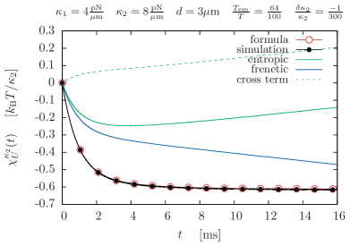
In our first example, we have the unperturbed force and we consider a perturbation on top of it. For the sake of having a scalar response function, let us assume and . That is, the “cooler” trap without the artificial noise is being perturbed. We then have for use in (the integral of) Eq. (30). As the observable of interest, we focus on the energy stored in the traps; the total energy and the energy stored in the first trap. In other words, we observed the susceptibilities
| (31) |
where the latter is interesting in that the first trap feels the perturbation on the second only via hydrodynamic coupling. The response in the first trap can be found simply by subtracting, .
 |
 |
Graphs for the susceptibilities are shown in Fig. 1, along with some technical details. At the initial time when the perturbation was turned on, the positions were effectively sampled from the nonequilibrium stationary state created by the presence of external noise on the first trap. In the example shown, the second trap was softened (), resulting in more spread of the particles, hence a larger positive value for the energies, and therefore a negative susceptibility after division by . In the bottom graph, we see how the first particle’s energy responds to a perturbation in the other trap. In particular, softening the cooler trap is seen to add energy to the warmer trap, via hydrodynamic coupling. The entropic and frenetic parts stray from each other in both observables. We have also plotted (dashed line) the part of the entropic response that is proportional to the off-diagonal entry (alternatively, according to Eq. (29a) or (30), this part arises from ). This cross-term appears to account for most of the response in the unperturbed trap, which is intuitive since the fluctuations here have to do eventually with the cross-correlation between the traps. In addition, the overall running-away between the entropic and frenetic parts appear to also be induced by this cross term. This point is further discussed in the following complementary case.
4.2.2 Perturbing the warmer trap
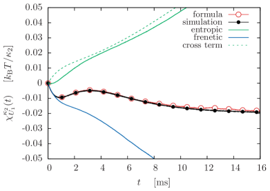
In the above example, we considered the case of the strength of the cooler optical trap being manipulated, where the perturbing force had and . Note that the nonzero component multiplies the off-diagonal entry of the inverse temperature matrix in products of the form of Eq. (29). As this off-diagonal entry is the main feature that distinguishes this nonequilibrium situation from those with decoupled reservoirs, we chose to deal with the case where this term is present first. However, the opposite case of manipulating the warmer trap has , which removes the off-diagonal entry from the evaluation of the response. Simulations pertaining to this case illustrate the distinction.

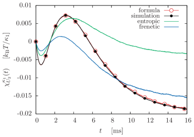
Fig. 2 depicts the associated susceptibilities of the total energy and the energy in the unperturbed trap, similar to the case above. Due to the softness of the warmer trap—which was an arbitrary choice of ours—the relaxation is seen to be slower than in the previous case. Here, we note that the runaway behaviour seen in the previous Fig. 1, of both the entropic and the frenetic parts, disappears along with the disappearance of the cross term in the inverse temperature matrix. For the entropic term, this corresponds to the removal of the cross term from the entropy production, the correlations with which had been depicted in dashed lines previously.
Following the discussion in Sec. 3.3, it is possible to argue that, at least for the case of separable potential that we have, this runaway behaviour, when it is present, has to do with the fact that the cross terms () constitute the residual housekeeping entropy production rate associated with the stationary nonequilibrium imposed by the broken proportionality between and : Each term of equals the rate of change of the energy stored in trap , which vanishes on the average in stationarity by definition, thereby rendering the remainder () proportional to the housekeeping dissipation on the average. In the present case of perturbing the warmer trap, it is the absence of correlations with (the excess in) this residual steady rate of entropy production that is apparently responsible for the disappearance of the runaway behaviour that was seen in the previous example. Similarly, the frenetic part is also stabilized or not depending on the absence of this cross term. A notion of frenetic housekeeping cost might be needed to account for this aspect.
5 Linear response: thermal perturbation
Here, we discuss the linear response to small variations in temperature, or equivalently the diffusion coefficients, in a scheme where we discretize time. A similar scheme was used in Ref. [31] for a single degree of freedom and adopting the Itô convention rather than the Stratonovich one. In the Appendix we discuss the unusual issue of needing to select from the start which convention to use, even if the stochastic equations have a constant noise prefactor.
We have seen above that how the continuum limit is taken becomes irrelevant as far as the response to mechanical perturbations was concerned, since the force-dependent terms of the action (24) are well-behaved. In contrast, we will see that varying the temperature or diffusion coefficients retains regularization-dependent parts of the action.
5.1 Response formulas
The variation of the action, Eq. (24) or (27), with respect to the diffusion matrix can be done as before by substitution () and sifting the linear order. Noting the following relations,
| (32a) | ||||
| (32b) | ||||
which can be confirmed easily by differentiating the definition , and using a Taylor series around for the logarithm, we find
| (33a) | ||||
| (33b) | ||||
Here, we have denoted as , and have refrained from substituting Eq. (32a), both for the sake of compactness. Also note that, similarly to the force perturbation case, the perturbation is in general a function of time. Finally, the first term of the symmetric part (33b)—that which depends on the regularization—has been written as a discrete sum over time slices, before the continuum limit is taken, in the spirit of Eq. (25). In the limit , the term as a result of the equation of motion to lowest order in , thereby negating the singularity coming from the normalization. Hence, the regularization-dependent term is expected to be at least as well-behaved as the stochastic integral of the entropic part (33a), with each increment being of the order .
The response function then has the form
| (34) |
where we have used a definition
| (35) |
for the regularization-dependent part. For the scenario at hand, a natural scalar parameter to perturb is the effective temperature .
5.2 Numerical experiments
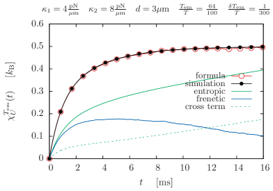
In order to check the response formulas above, we performed numerical simulations considering a perturbation applied in a stepwise fashion on our paradigmatic system in a stationary state corresponding to the original effective temperature . Considering the total energy as the observable, one obtains a susceptibility akin to a heat capacity by integrating the response function (34). The inverse of the diffusion matrix (14) for our example is found as
| (36) |
which implies (with )
| (37) |
to be used in Eq. (34).
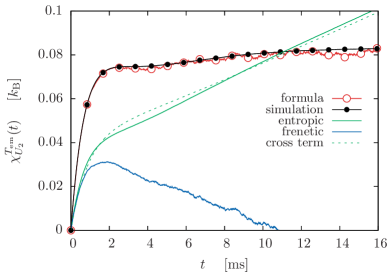
In the simulations, as before, we measured the susceptibilities of both the total energy , and the energy in the unperturbed trap, to validate the response formulas. In other words, we verified the susceptibilities and . The second susceptibility, as before, is interesting in that it is only due to hydrodynamic coupling that there is a nonzero response in this trap, as there is no mechanical coupling between the two particles. In Fig. 3 we see the susceptibilities upon an increase in the effective temperature of the external noise. The increase in the energy stored in the cooler trap due to the increased temperature difference occurs faster, since the cooler trap was arbitrarily chosen to be stiffer. We observe again that the entropic and frenetic parts diverge from each other. The parts of entropic response involving the cross-term were plotted in dashed lines, and it is seen, as before, that this part constitutes most of the response in the unperturbed trap and also that it is responsible for the run-away of the entropic part.
6 Conclusions
To sum up, we have investigated a physical situation where microscopic colloidal particles in solvent are held close to each other, enough to experience hydrodynamically mediated correlations in their fluctuation. We derived the response to small perturbations of deterministic or thermal origin, within a path-weight framework. An experiment [1] that traps the colloids at a more or less fixed distance is suitable for studying the influence of hydrodynamic coupling in isolation from other potential complications. Despite this simplification, we deal with a system driven out of equilibrium by unbalanced thermal reservoir influences, in the form of one degree of freedom being “heated up” by an artificial noise. This is absorbed into the diffusion matrix of a stochastic equation and leads to a non-diagonal “inverse temperature matrix” . Hence, the reservoir cannot be thought of as comprising components that thermalize each degree of freedom separately. A complex condition thus arises from mixing hydrodynamic interactions with the action of a nonequilibrium heat bath. There is no well-defined equilibrium temperature to scale the heat exchanges that would yield the change of entropy in the reservoir. Hence, notions as heat, power delivered, entropy, etc. need to be considered with care.
We found it more convenient to continue using the term “entropy production” for the time-antisymmetric dimensionless objects emerging from path-weights. However, this should be considered more a concession to acknowledging the property of this objects to detect time-reversal breaking rather than being true equilibrium thermodynamic entropy changes in the reservoirs. In particular, attempting to identify entropy fluxes into reservoirs is compromised by off-diagonal entries of the inverse temperature matrix endowed by the nonequilibrium heat bath with hydrodynamic coupling: Cross terms of the form () contribute as well to our results. While it is tempting to ascribe a meaning to such forms along the lines of power transfer between and , we have argued that they are rather indicators of the departure from equilibrium conditions. Since stationary averages of do vanish, the non-zero cross term should be in close relationship with the notion of housekeeping dissipation, necessary to maintain the nonequilibrium condition . It is thus possible to argue that the measurements of Ref. [1] can be interpreted as indicators of the housekeeping dissipation. Since we deal also with time-symmetric quantities, possibly concepts as housekeeping frenesy should be introduced to pair with that of housekeeping heat.
Within the path probability framework, we derived explicit expressions for the linear response of such a system to changes in the deterministic forces as well as thermal influences acting on the particles. It should be possible to verify these expressions in experiments measuring particle trajectories [1], just by following the scheme of our simulations, which perturbed either the trap strengths or the magnitude of the artificial noise (temperature).
The fixed distance between the traps allowed an approximation where diffusion and mobility coefficients were independent of coordinates. In more general situations, such as the motion of a collection of active Brownian particles, or colloidal model systems where particles are not necessarily fixed, this needs to be incorporated. It is not clear how the phase behaviour or linear response would be influenced in systems where the coordinate dependence of the reservoir forces becomes relevant.
Regarding the regularization-dependence of the temperature response formulas, Eqs. (34) and (35), we note that a reparametrization of the degrees of freedom such as that suggested in Refs. [46, 47] can remove it. This will be investigated in a future work.
Appendix: Itô and Euler vs. Stratonovich and Heun
In numerical computations, it is important to ensure consistency between the numerical integration that generates trajectories and the interpretation of the stochastic equation of motion [35], which in turn determines the form of the path weights. Accordingly, overdamped motion was generated in the simulations of Ref. [31] via (explicit) Euler integration, matching their choice of Itô convention for expressing the path weights. In the present article, instead, we adopt the Stratonovich convention for reasons explained at the beginning of Sec. 3.2. Therefore, the numerical integration we used for generating stochastic trajectories was based on Heun’s method, which is a type of semi-implicit Euler scheme agreeing with the Stratonovich interpretation, to order [35, 44]. However, it seems odd that in a scenario with state-independent coefficients this issue would become relevant.
Nonetheless, one can easily check numerically that if an Euler scheme rather than Heun is used to generate the trajectories, data depart from our analytical results in the case of temperature response. Furthermore, and somewhat surprisingly, it is not possible to shift between the two noise interpretations in the final expressions for the response in order to recover agreement: Notice that due to its lack of temperature dependence, the temperature derivative erases the last term of the path action (24), which however has to be involved in any alteration of the noise interpretation. Even though a conversion of the stochastic integrals is still permissible after this point, the trajectories must be generated by numerics respecting the original convention. Indeed, the overdamped trajectories of Ref. [31] were generated using an Euler scheme notwithstanding the final conversion of stochastic integrals from Itô to Stratonovich, which was done in order to define the time-symmetry of the integrals.
A heuristic justification of such discrepancy despite the state-independence of noise coefficients is the following: Typically, agreement between the noise interpretation and stochastic integration is sought in the path increments to order . However, in our scheme we deal with path weights that eventually rely on the square of path increments to order . As a result, any disagreement between the stochastic interpretation and integration at order of the path increment will introduce error, even if constant coefficients ensure agreement at order . Although we have not carried out a rigorous proof showing what the terms of order might be, it appears that the same rule of thumb prescribing semi-implicit integration to accompany Stratonovich interpretation appears to remain valid.
References
References
- [1] Bérut A, Petrosyan A and Ciliberto S 2014 Europhys. Lett. 107 60004
- [2] Doi M and Edwards S 1988 The Theory of Polymer Dynamics (Clarendon Press)
- [3] Ramaswamy S 2010 The mechanics and statistics of active matter (Annual Review of Condensed Matter Physics vol 1) ed Langer J p 323
- [4] Bialke J, Speck T and Loewen H 2012 Phys. Rev. Lett. 108 168301
- [5] Buttinoni I, Bialke J, Kuemmel F, Loewen H, Bechinger C and Speck T 2013 Phys. Rev. Lett. 110 238301
- [6] Wang G, Sevick E, Mittag E, Searles D and Evans D 2002 Phys. Rev. Lett. 89 050601
- [7] Trepagnier E, Jarzynski C, Ritort F, Crooks G, Bustamante C and Liphardt J 2004 Proc. Natl. Acad. Sci. 101 15038
- [8] Blickle V, Speck T, Helden L, Seifert U and Bechinger C 2006 Phys. Rev. Lett. 96
- [9] Blickle V, Speck T, Seifert U and Bechinger C 2007 Phys. Rev. E 75 060101(R)
- [10] Blickle V, Speck T, Lutz C, Seifert U and Bechinger C 2007 Phys. Rev. Lett. 98 210601
- [11] Lutz C, Reichert M, Stark H and Bechinger C 2006 Europhys. Lett. 74 719
- [12] Gomez-Solano J R, Petrosyan A, Ciliberto S, Chetrite R, and Gawȩdzki K 2009 Phys. Rev. Lett. 103 040601
- [13] Kotar J, Leoni M, Bassetti B, Cosentino Lagomarsino M and Cicuta P 2010 Proc. Natl. Acad. Sci. 107 7669–7673
- [14] Kubo R 1966 Rep. Prog. Phys. 29 255–284
- [15] Baiesi M, Maes C and Wynants B 2009 Phys. Rev. Lett. 103 010602
- [16] Baiesi M and Maes C 2013 New J. Phys. 15 013004
- [17] Marini Bettolo Marconi U, Puglisi A, Rondoni L and Vulpiani A 2008 Phys. Rep. 461 111–195
- [18] Agarwal G S 1972 Z. Physik 252 25–38
- [19] Falcioni M, Isola S and Vulpiani A 1990 Phys. Lett. A 144 341
- [20] Seifert U and Speck T 2010 Europhys. Lett. 89 10007
- [21] Cugliandolo L, Kurchan J and Parisi G 1994 J. Phys. I 4 1641
- [22] Lippiello E, Corberi F and Zannetti M 2005 Phys. Rev. E 71 036104
- [23] Baiesi M, Maes C and Wynants B 2009 J. Stat. Phys. 137 1094–1116
- [24] Baiesi M, Boksenbojm E, Maes C and Wynants B 2010 J. Stat. Phys. 139 492–505
- [25] Basu U and Maes C 2015 J. Phys. Conference Series 638 012001
- [26] Lecomte V, Appert-Rolland C and van Wijland F 2005 Phys. Rev. Lett. 95 010601
- [27] Merolle M, Garrahan J P and Chandler D 2005 Proc. Natl. Acad. Sci. 102 10837–10840
- [28] Garrahan J P, Jack R L, Lecomte V, Pitard E, van Duijvendijk K and van Wijland F 2007 Phys. Rev. Lett. 98 195702
- [29] Lepri S, Livi R and Politi A 2003 Phys. Rep. 377 1–80
- [30] Dhar A 2008 Adv. Phys. 57 457–537
- [31] Baiesi M, Basu U and Maes C 2014 Eur. Phys. J. B 87 277
- [32] Oono Y and Paniconi M 1998 Progr. Theor. Phys. Suppl. 130 29–44
- [33] Hatano T and Sasa S 2001 Phys. Rev. Lett. 86 3463––3466
- [34] Speck T and Seifert U 2006 Europhys. Lett. 74 391–396
- [35] Gardiner C W 2004 Handbook of stochastic methods for physics, chemistry and the natural sciences 3rd ed (Springer Series in Synergetics vol 13) (Berlin: Springer-Verlag) ISBN 3-540-20882-8
- [36] Tokuyama M and Oppenheim I 1994 Phys. Rev. E 50 R16
- [37] Tokuyama M and Oppenheim I 1995 Physica A 216 85
- [38] Rotne J and Prager S 1969 J. Chem. Phys. 50 4831
- [39] Martínez I A, Roldán E, Parrondo J M R and Petrov D 2013 Phys. Rev. E 87 032159
- [40] Lebowitz J L and Spohn H 1999 J. Stat. Phys. 95 333–365
- [41] Maes C 1999 J. Stat. Phys. 95 367–392
- [42] Arnold P 2000 Phys. Rev. E 61 6099
- [43] Langouche F, Roekaerts D and Tirapegui E 1982 Functional integration and semiclassical expansions (Dordrecht: Reidel)
- [44] Sekimoto K 2010 Stochastic Energetics (Lecture Notes in Physics vol 799) (Springer)
- [45] Maes C 2012 Physica Scripta 86 058509
- [46] Falasco G and Baiesi M 2016 Europhys. Lett. 113 20005
- [47] Falasco G and Baiesi M 2016 arXiv:1601.06958