Tensor decomposition and homotopy continuation

Abstract

A computationally challenging classical elimination theory problem is to compute polynomials which vanish on the set of tensors of a given rank. By moving away from computing polynomials via elimination theory to computing pseudowitness sets via numerical elimination theory, we develop computational methods for computing ranks and border ranks of tensors along with decompositions. More generally, we present our approach using joins of any collection of irreducible and nondegenerate projective varieties $X_{1},\ldots,X_{k}\subset{\mathbb{P}}^{N}$ defined over ${\mathbb{C}}$. After computing ranks over ${\mathbb{C}}$, we also explore computing real ranks. A variety of examples are included to demonstrate the numerical algebraic geometric approaches.

Key words and phrases. tensor rank, homotopy continuation, numerical elimination theory, witness sets, numerical algebraic geometry, joins, secant varieties.

2010 Mathematics Subject Classification. Primary 65H10; Secondary 13P05, 14Q99, 68W30.

Introduction

Computing tensor decompositions is a fundamental problem in numerous application areas including computational complexity, signal processing for telecommunications [36, 46], scientific data analysis [63, 84], electrical engineering [33], and statistics [72]. Some other applications include the complexity of matrix multiplication [92], the complexity problem of P versus NP [94], the study of entanglement in quantum physics [48], matchgates in computer science [94], the study of phylogenetic invariants [6], independent component analysis [35], blind identification in signal processing [83], branching structure in diffusion images [81], and other multilinear data analytic techniques in bioinformatics and spectroscopy [37].

One computational algebraic geometric approach for deciding if a decomposition can exist is to compute equations that define secant and join varieties (e.g., see [66, Chap. 7] for a general overview). This can be formulated as a classical elimination theory question which, at least in theory, can be computed using Gröbner basis methods. Moreover, the defining equations do not yield decompositions, only existential information. Rather than focusing on computing defining equations, this paper uses numerical algebraic geometry (e.g, see [14, 90] for a general overview) for performing membership tests and computing decompositions. In particular, we use numerical elimination theory to perform the computations based on the methods developed in [57, 58] (see also [14, Chap. 16]). This approach differs from several previous methods of combining numerical algebraic geometry and elimination theory, e.g., [12, § 3.3-3.4] and [88, 89], in that these previous methods relied upon interpolation.

The general setup for this paper is as follows. Let $X\subset{\mathbb{P}}^{N}$ be an irreducible and nondegenerate projective variety defined over ${\mathbb{C}}$ and ${\mathcal{C}}(X)\subset{\mathbb{C}}^{N+1}$ be the affine cone of $X$. We let a point $P$ be a nonzero vector in $\mathbb{C}^{N+1}$ while $[P]$ denotes the line in $\mathbb{C}^{N+1}$ passing through the origin and $P$, i.e., $[P]\in{\mathbb{P}}^{N}$ is the projectivization of $P\in{\mathbb{C}}^{N+1}$. The $X$-rank of $[P]\in\mathbb{P}^{N}$ (or of $P\in{\mathbb{C}}^{N+1}$), denoted $\operatorname{rk}_{X}(P)$, is the minimum $r\in\mathbb{N}$ such that $P$ can be written as a linear combination of $r$ elements of ${\mathcal{C}}(X)$:

$$P=\sum_{i=1}^{r}x_{i},\;\;\;x_{i}\in{\mathcal{C}}(X).$$ (1)

Let $\sigma_{r}^{0}(X)\subset{\mathbb{P}}^{N}$ denote the set of elements with rank at most $r$ and, for $[x_{i}]\in{\mathbb{P}}^{N}$, let $\langle[x_{1}],\ldots,[x_{r}]\rangle$ denoted the linear space spanned by $x_{1},\dots,x_{r}$. The $r^{\rm th}$ secant variety of $X$ is

$$\sigma_{r}(X)=\overline{\sigma_{r}^{0}(X)}=\overline{\bigcup_{[x_{1}],\ldots,[x_{r}]\in X}\langle[x_{1}],\ldots,[x_{r}]\rangle}.$$

In particular, if ${[P]}\in\sigma_{r}(X)$, then $[P]$ is the limit of a sequence of elements of $X$-rank at most $r$. The $X$-border rank of ${[P]}$, denoted $\operatorname{brk}_{X}(P)$, is the minimum $r\in{\mathbb{N}}$ such that ${[P]}\in\sigma_{r}(X)$. Obviously, $\operatorname{brk}_{X}({P})\leq\operatorname{rk}_{X}({P})$.

Secant varieties are just special cases of join varieties. For irreducible and nondegenerate projective varieties $X_{1},\ldots,X_{k}$, the constructible join and join variety of $X_{1},\ldots,X_{k}$, respectively, are

$$J^{0}(X_{1},\ldots,X_{k})=\bigcup_{[x_{1}]\in X_{1},\ldots,[x_{k}]\in X_{k}}\langle[x_{1}],\ldots,[x_{k}]\rangle\hbox{~{}~{}and~{}~{}}J(X_{1},\ldots,X_{k})=\overline{J^{0}(X_{1},\ldots,X_{k})}.$$ (2)

Clearly, $\sigma_{r}^{0}(X)=J^{0}(\underbrace{X,\ldots,X}_{r})$ and $\sigma_{r}(X)=J(\underbrace{X,\ldots,X}_{r})$.

As mentioned above, one can test, in principle, if an element belongs to a certain join variety (or if it has certain $X$-border rank) by computing defining equations for the join variety (or the secant variety, respectively). Unfortunately, finding defining equations for secant and join varieties is generally a very difficult elimination problem which is far from being well understood at this time.

The following summarizes the remaining sections of this paper.

The knowledge of whether an element lies in a constructible join (or if it has a certain $X$-rank) is an open condition. In fact, $\sigma_{r}^{0}(X)$ is almost always an open subset of $\sigma_{r}(X)$, so membership tests for $\sigma_{r}^{0}(X)$ based on evaluating polynomials to determine the $X$-rank of a given element do not exist in general. Currently, there are few theoretical algorithms for specific cases, e.g., [10, 17, 18, 28, 34, 62, 74, 93]. In Section 1, we present a numerical algebraic geometric approach to join varieties.

Once an element is known to be in $J(X_{1},\dots,X_{k})$ or $\sigma_{r}(X)$, numerical elimination theory can also be used to decide if the element is in the corresponding constructible set $J^{0}(X_{1},\dots,X_{k})$ or $\sigma_{r}^{0}(X)$. Rather than test a particular element, Section 2 considers the approach first presented in [57] for computing the codimension one components of the boundaries of $J^{0}(X_{1},\dots,X_{k})$ or $\sigma_{r}^{0}(X)$, namely the codimension one components of $\overline{{J(X_{1},\dots,X_{k})}\setminus{J^{0}(X_{1},\dots,X_{k})}}$ and $\overline{{\sigma_{r}(X)}\setminus{\sigma_{r}^{0}(X)}}$. For example, this allows one to compute the codimension one component of the closure of the set of points of $X$-border rank at most $r$ whose rank is strictly larger than $r$.

Another problem considered in this paper from the numerical point of view regards computing real decompositions of a real element. For example, after computing the $X$-rank $r$ of a real element ${P}$, we would like to know if it has a decomposition using $r$ real elements, that is, determine if the real $X$-rank of $P$ is the same as its complex $X$-rank. Computing the real $X$-rank has recently been studied by various authors, especially in regards to the typical ranks of symmetric tensors, i.e., $r$ such that the symmetric tensors whose real rank is $r$ is an open real set. Theoretic results in this direction are provided in [8, 11, 20, 24, 26, 32, 38]. In Section 3, we describe a method using [51] to determine the existence of real decompositions.

We emphasize that a numerical algebraic geometric approach works well for decomposing generic elements. For example, a numerical algebraic geometric based approach was presented in [56] for computing the total number of decompositions of a general element in the so-called perfect cases, i.e., when the general element has finitely many decompositions. In every case, one can track a single solution path defined by a Newton homotopy to compute a decomposition of a general element, as shown in Section 4.

Local numerical techniques exist for computing (numerically approximating) decompositions of elements, e.g., see [65, 85]. Section 4 also develops an approach for combining such local numerical techniques with Newton homotopies for deriving upper bounds on border rank over both the real and complex numbers.

The last section, Section 5, considers a variety of examples.

1 Membership tests

Let $X_{1},\dots,X_{k}\subset{\mathbb{P}}^{N}$ be irreducible and nondegenerate projective varieties. Consider the constructible join $J^{0}(X_{1},\dots,X_{k})$ and join variety $J(X_{1},\dots,X_{k})$ defined in (2). One key aspect of this numerical algebraic geometric approach is to consider the smooth irreducible variety, called the abstract join variety,

$${\mathcal{J}}=\left\{({[P]},x_{1},\dots,x_{k})~{}\left|~{}x_{i}\in{\mathcal{C}}(X_{i}),P=\sum_{i=1}^{k}x_{i}\right\}\right.\subset{\mathbb{P}}^{N}\times{\mathcal{C}}(X_{1})\times\cdots\times{\mathcal{C}}(X_{k}),$$ (3)

where ${\mathcal{C}}(X_{i})$ is the affine cone of $X_{i}$. For the projection $\pi({[P]},x_{1},\dots,x_{k})={[P]}$, it is clear that

$$\pi({\mathcal{J}})=J^{0}(X_{1},\dots,X_{k})\hbox{~{}~{}and~{}~{}}\overline{\pi({\mathcal{J}})}=J(X_{1},\dots,X_{k}).$$ (4)

The key to using the numerical elimination theory approaches of [57, 58] is to perform all computations on the abstract join variety ${\mathcal{J}}$. Moreover, one only needs a numerical algebraic geometric description, i.e., a witness set or a pseudowitness set, which we define in Section 1.1, of each irreducible variety $X_{i}$ to perform such computations on ${\mathcal{J}}$.

Since ${\mathcal{J}}$ naturally depends on affine cones, we will simplify the numerical algebraic geometric presentation by just considering affine varieties. As [58, Remark 8] states, we can naturally extend from affine varieties to projective spaces by considering coordinates as sections of the hyperplane section bundle and accounting for the fact that coordinatewise projections have a center, i.e., a set of indeterminacy, that is contained in each fiber. Another option is to restrict to a general affine coordinate patch and introduce scalars as illustrated in Section 1.3. Due to this implementation choice, there is the potential for ambiguity in Section 1.2, e.g., the dimension of the affine cone over a projective variety is one more than the dimension of the projective variety. In that section, the meaning of dimension is dependent on the implementation choice.

After defining witness sets, we explore a membership test for the join variety $J(X_{1},\dots,X_{k})$ in Section 1.2. This test uses homotopy continuation without the need for computing defining equations, e.g., via interpolation or classical elimination, for $J(X_{1},\dots,X_{k})$.

1.1 Witness and pseudowitness sets

The fundamental data structure in numerical algebraic geometry is a witness set, with numerical elimination theory relying on pseudowitness sets first described in [58]. For simplicity, we provide a brief overview of both in the affine case with more details available in [14, Chap. 8 & 16].

Let $X\subset{\mathbb{C}}^{N}$ be an irreducible variety. A witness set for $X$ is a triple $\{f,{\mathcal{L}},W\}$ where $f\subset{\mathbb{C}}[x_{1},\dots,x_{N}]$ such that $X$ is an irreducible component of $\mathcal{V}(f)=\{x\in{\mathbb{C}}^{N}~{}|~{}f(x)=0\}$, ${\mathcal{L}}$ is a linear space in ${\mathbb{C}}^{N}$ with $\dim{\mathcal{L}}=\operatorname{codim}X$ which intersects $X$ transversally, and $W:=X\cap{\mathcal{L}}$. In particular, $W$ is a collection of $\deg X$ points in ${\mathbb{C}}^{N}$, called a witness point set.

If the multiplicity of $X$ with respect to $f$ is greater than $1$, we can use, for example, isosingular deflation [61] or a symbolic null space approach of [55], to replace $f$ with another polynomial system $f^{\prime}\subset{\mathbb{C}}[x_{1},\dots,x_{N}]$ such that $X$ has multiplicity $1$ with respect to $f^{\prime}$. Therefore, without loss of generality, we will assume that $X$ has multiplicity $1$ with respect to its witness system $f$. That is, $\dim X=\dim\operatorname{null}Jf(x^{*})$ for general $x^{*}\in X$ where $Jf$ is the Jacobian matrix of $f$.

Example 1

For illustration, consider the irreducible variety $X:=\mathcal{V}(f)\subset{\mathbb{C}}^{3}$ where $f=\{x_{1}^{2}-x_{2},x_{1}^{3}+x_{3}\}$. The triple $\{f,{\mathcal{L}},W\}$ forms a witness set for $X$ where ${\mathcal{L}}:=\mathcal{V}(2x_{1}-3x_{2}-5x_{3}+1)$ and $W:=X\cap{\mathcal{L}}$ which, to 3 decimal places, is the following set of three points:

$$\left\{\begin{array}[]{l}(-0.299,0.089,0.027),(0.450\pm 0.683\cdot\sqrt{-1},-0.265\pm 0.614\cdot\sqrt{-1},0.539\mp 0.095\cdot\sqrt{-1})\end{array}\right\}$$

We note that ${\mathcal{L}}$ was defined using small integer coefficients for presentation purposes while, in practice, such coefficients are selected in the complex numbers using a random number generator.

A witness set for $X$ can be used to decide membership in $X$ [88]. Suppose that $p\in{\mathbb{C}}^{N}$ and ${\mathcal{L}}_{p}\subset{\mathbb{C}}^{N}$ is a linear space passing through $p$ which is transverse to $X$ at $p$ with $\dim{\mathcal{L}}_{p}=\dim{\mathcal{L}}=\operatorname{codim}X$. With this setup, $p\in X$ if and only if $p\in X\cap{\mathcal{L}}_{p}$ which can be decided by deforming from $X\cap{\mathcal{L}}$. That is, one computes the convergent endpoints, at $t=0$, of the $\deg X$ paths starting, at $t=1$, from the points in $W$ defined by the homotopy $X\cap(t\cdot{\mathcal{L}}+(1-t)\cdot{\mathcal{L}}_{p})$. In particular, $p\in X$ if and only if $p$ arises as an endpoint.

Suppose now that $\pi:{\mathbb{C}}^{N}\rightarrow{\mathbb{C}}^{M}$ is the projection defined by $\pi(x_{1},\dots,x_{N})=(x_{1},\dots,x_{M})$ and $Y:=\overline{\pi(X)}\subset{\mathbb{C}}^{M}$. Consider the matrix $B=[I_{M}~{}0]\in{\mathbb{C}}^{M\times N}$ so that $\pi(x)=Bx$. A pseudowitness set for $Y$ [58] is a quadruple $\{f,\pi,{\mathcal{M}},U\}$ which is built from a witness set for $X$, namely $\{f,{\mathcal{L}},W\}$, as follows. First, one computes the dimension of $Y$, for example, using [58, Lemma 3], namely

$$\dim Y=\dim X-\dim\operatorname{null}\left[\begin{array}[]{c}Jf(x^{*})\\ B\end{array}\right]$$ (5)

for general $x^{*}\in X$.

Suppose that ${\mathcal{M}}_{1}\subset{\mathbb{C}}^{M}$ is a general linear space with $\dim{\mathcal{M}}_{1}=\operatorname{codim}Y$ and ${\mathcal{M}}_{2}\subset{\mathbb{C}}^{N}$ is a general linear space with $\dim{\mathcal{M}}_{2}=\operatorname{codim}X-\operatorname{codim}Y=:\dim_{gf}(X,\pi)$, i.e., the dimension of a general fiber of $X$ with respect to $\pi$. Let ${\mathcal{M}}:=({\mathcal{M}}_{1}\times{\mathbb{C}}^{N-M})\cap{\mathcal{M}}_{2}$. We assume that ${\mathcal{M}}_{1}$ and ${\mathcal{M}}_{2}$ are chosen to be sufficiently general so that $\dim{\mathcal{M}}=\dim{\mathcal{L}}=\operatorname{codim}X$ and $U:=X\cap{\mathcal{M}}$ consists of $\deg Y\cdot\deg_{gf}(X,\pi)$ points where $\deg_{gf}(X,\pi)$ is the degree of a general fiber of $X$ with respect to $\pi$. Thus, for the pseudowitness point set $U$, $\deg Y=|\pi(U)|$ and $\deg_{gf}(X,\pi)=|U|/|\pi(U)|$.

Remark 2

Relation (5) provides an approach for determining if the join variety is defective, i.e., smaller than the expected dimension. In fact, since the abstract join ${\mathcal{J}}$ of (3) always has the expected dimension, namely $\sum_{i=1}^{k}\dim X_{i}$, we may take $Y$ to be the join so that $X={\mathcal{J}}$ with $Y=\overline{\pi({\mathcal{J}})}$.

Example 3

Continuing with the setup from Ex. 1, consider the map $\pi(x_{1},x_{2},x_{3})=(x_{1},x_{2})$. Clearly, $Y:=\overline{\pi(X)}$ is the parabola defined by $x_{2}=x_{1}^{2}$, but we will proceed from the witness set for $X$ to construct a pseudowitness set for $Y$.

We have

$$B=\left[\begin{array}[]{ccc}1&0&0\\ 0&1&0\end{array}\right]\hbox{~{}~{}and~{}~{}}\dim\operatorname{null}\left[\begin{array}[]{ccc}2x_{1}^{*}&-1&0\\ 0&3(x_{1}^{*})^{2}&x_{3}^{*}\\ 1&0&0\\ 0&1&0\end{array}\right]=0\hbox{~{}for general~{}}(x_{1}^{*},x_{2}^{*},x_{3}^{*})\in X.$$

Thus, $\dim Y=\dim X=1$ and we can take ${\mathcal{M}}:=\mathcal{V}(2x_{1}-3x_{2}+1)\times{\mathbb{C}}\subset{\mathbb{C}}^{3}$.

We can compute the pseudowitness point set $U:=X\cap{\mathcal{M}}$ starting from the three points in $W=X\cap{\mathcal{L}}$ using the homotopy defined by $X\cap(t\cdot{\mathcal{L}}+(1-t)\cdot{\mathcal{M}})$. For this homotopy, two paths converge and one diverges where the two convergent endpoints forming $U$ are

$$(1,1,-1),~{}~{}~{}~{}(-1/3,1/9,1/27).$$

In particular, $\deg Y=|\pi(U)|=2$ and $\deg_{gf}(X,\pi)=|U|/|\pi(U)|=1$, meaning that $\pi$ is generically a one-to-one map from $X$ to $Y$.

Example 4

As an example of computing a pseudowitness set for a join of varieties which are not rational, we consider curves $C_{i}\in{\mathbb{P}}^{4}$ which are defined by the intersection of $3$ random quadric hypersurfaces. Hence, $C_{i}=\mathcal{V}(f_{i1},f_{i2},f_{i3})$ where $f_{ij}$ has degree $2$ so that each $C_{i}$ is a complete intersection with $\deg C_{i}=2^{3}=8$. Consider the abstract joins

$$\begin{array}[]{rcl}{\mathcal{J}}_{12}&=&\{([P],x_{1},x_{2})~{}|~{}P=x_{1}+x_{2},f_{ij}(x_{i})=0\hbox{~{}for~{}}i=1,2\hbox{~{}and~{}}j=1,2,3\},\\ {\mathcal{J}}_{11}&=&\{([P],x_{1},x_{2})~{}|~{}P=x_{1}+x_{2},f_{1j}(x_{i})=0\hbox{~{}for~{}}i=1,2\hbox{~{}and~{}}j=1,2,3\}.\end{array}$$

That is, for $\pi([P],x_{1},x_{2})=[P]$, we have $\overline{\pi({\mathcal{J}}_{12})}=J(C_{1},C_{2})$ and $\overline{\pi({\mathcal{J}}_{11})}=J(C_{1},C_{1})=\sigma_{2}(C_{1})$.

Witness sets for ${\mathcal{J}}_{12}$ and ${\mathcal{J}}_{11}$ show that both abstract join varieties have degree $64$. Then, by converting from a witness set to a pseudowitness set as described above, we find that $J(C_{1},C_{2})$ is a hypersurface of degree $64$ while $\sigma_{2}(C_{1})$ is a hypersurface of degree $16$ with $\deg_{gf}({\mathcal{J}}_{11},\pi)=2$.

Example 5

A key component of the proof of [70, Thm. 1] is computing the dimension of

$$Y=\overline{\left\{x_{hi}^{11}x_{jk}^{12}x_{\ell m}^{13}+x_{hi}^{21}x_{jk}^{22}x_{\ell m}^{23}~{}\left|~{}x_{\alpha\beta}^{\gamma\delta}\in{\mathbb{C}},~{}h,i,j,k,\ell,m\in\{0,1\},~{}i+k+m\equiv 0\mbox{~{}mod~{}}2\right\}\right.}\subset{\mathbb{C}}^{32}$$

We can compute $\dim Y$ using (5) as follows. Let $X=\mathcal{V}(f)\subset{\mathbb{C}}^{32}\times{\mathbb{C}}^{24}$ where

$$f(z,x)=\left[\begin{array}[]{c}x_{hi}^{11}x_{jk}^{12}x_{\ell m}^{13}+x_{hi}^{21}x_{jk}^{22}x_{\ell m}^{23}-z_{hijk\ell m}\\ h,i,j,k,\ell,m\in\{0,1\},~{}i+k+m\equiv 0\mbox{~{}mod~{}}2\end{array}\right]$$

and $\pi(z,x)=z$ so that $Y=\overline{\pi(X)}$ and $B=[I_{32}~{}0]$. Thus, for general $x^{*}\in{\mathbb{C}}^{24}$ with $z^{*}\in{\mathbb{C}}^{32}$ such that $f(z^{*},x^{*})=0$, we have

$$\dim Y=\dim X-\dim\operatorname{null}\left[\begin{array}[]{c}Jf(z^{*},x^{*})\\ B\end{array}\right]=24-\dim\operatorname{null}J_{x}f(x^{*})=24-4=20$$

where $J_{x}f(x)$ is the Jacobian matrix of $f$ with respect to $x$ which only depends on $x$. In fact, this is the largest dimension possible since $Y$ arises as a projection of $\sigma_{2}({\mathbb{C}}^{4}\times{\mathbb{C}}^{4}\times{\mathbb{C}}^{4})$ with $\dim\sigma_{2}({\mathbb{C}}^{4}\times{\mathbb{C}}^{4}\times{\mathbb{C}}^{4})=20$.

In practice, we may compute a pseudowitness point set $U$ by starting with one sufficiently general point in the image and performing monodromy loops. Such an approach has been used in various applications, e.g., [45, 71], and will be used in many of the examples in Section 5. Since $Y=\overline{\pi(X)}$, we can compute a general point $y\in Y$ given a general point $x\in X$. Then, pick a general linear space $L$ passing through $y$ so that $y\in U=Y\cap L$. A random monodromy loop consists of two steps, each of which is performed using a homotopy. First, we move $L$ to some other general linear space $L^{\prime}$. Next, we move back to $L$ via a randomly chosen path. During this loop, the path starting at $y\in U$ may arrive at some other point in $U$. We repeat this process until no new points are found for several loops. The completeness of the set is verified via a trace test. More information about this procedure can be found in, e.g., [45, 71] and [42, § 2.4.2].

The following discusses extending the membership test from witness sets to pseudowitness sets.

1.2 Membership test for images

As mentioned above, we can extend the notion of pseudowitness sets from the affine to the projective case. For the join variety $J:=J(X_{1},\dots,X_{k})=\overline{\pi({\mathcal{J}})}$ where ${\mathcal{J}}$ is the abstract join variety, we will simply assume that we have a pseudowitness set $\{f,\pi,{\mathcal{M}},U\}$ for $J$. This pseudowitness set for $J$ provides the required information needed to decide membership in the join variety [57]. As with the membership test using a witness set, testing membership in $J$ requires the tracking of at most $\deg J$ many paths, i.e., one only needs $U^{\prime}\subset U$ with $\pi(U^{\prime})=\pi(U)$ as discussed in [57, Remark 2].

Let $d:=\dim J$ and suppose that ${\mathcal{M}}_{1}$ is the corresponding sufficiently general codimension $d$ linear space from the pseudowitness set with $\pi(U)=\pi(U^{\prime})=J\cap{\mathcal{M}}_{1}$.

Given a point $[P]\in J$, suppose that ${\mathcal{L}}_{P}$ is a sufficiently general linear space of codimension $d$ passing through $[P]$. As with the membership test using a witness set, we want to compute $J\cap{\mathcal{L}}_{p}$ from $J\cap{\mathcal{M}}_{1}$. That is, we consider the $\deg J$ paths starting, at $t=1$, from the points in $\pi(U^{\prime})=\pi(U)$ defined by $J\cap(t\cdot{\mathcal{M}}_{1}+(1-t)\cdot{\mathcal{L}}_{P})$. Since polynomials vanishing on $J$ are not accessible, we use the pseudowitness set for $J$ to lift these paths to the abstract join variety ${\mathcal{J}}$ which, by assumption, is an irreducible component of $\mathcal{V}(f)$. Thus, $f$ permits path tracking on the abstract join variety ${\mathcal{J}}$ and hence permits the tracking along the join variety $J$. Given $w\in U^{\prime}$, let $Z_{w}(t)$ denote the path defined on ${\mathcal{J}}$ where $Z_{w}(1)=w$. In particular, we only need to consider $U^{\prime}\subset U$ since, for any $w^{\prime}\in U$ with $\pi(w)=\pi(w^{\prime})$, $\pi(Z_{w}(t))=\pi(Z_{w^{\prime}}(t))$. With this setup we have the following membership test, which is an expanded version of [57, Lemma 1].

Proposition 6

For the setup described above with $J^{0}:=J^{0}(X_{1},\dots,X_{k})$, the following hold.

1. $[P]\in J$ if and only if there exists $w\in U^{\prime}$ such that $\lim_{t\rightarrow 0}\pi(Z_{w}(t))=[P]$. Moreover, the multiplicity of $[P]$ with respect to $J$ is equal to $\left|\{w\in U^{\prime}~{}|~{}\lim_{t\rightarrow 0}\pi(Z_{w}(t))=[P]\}\right|$.

2. $[P]\in J^{0}$ if there exists $w\in U$ such that $\lim_{t\rightarrow 0}\pi(Z_{w}(t))=[P]$ and $\lim_{t\rightarrow 0}Z_{w}(t)\in{\mathcal{J}}$.

3. If, for every $w\in U^{\prime}$, $\lim_{t\rightarrow 0}Z_{w}(t)\in{\mathcal{J}}$, then $[P]\in J^{0}$ if and only if there exists $w\in U^{\prime}$ such that $\lim_{t\rightarrow 0}\pi(Z_{w}(t))=[P]$.

4. Let $E_{P}=\{w\in U~{}|~{}[P]=\lim_{t\rightarrow 0}\pi(Z_{w}(t))\}$. If $E_{P}\neq\emptyset$ and $\lim_{t\rightarrow 0}Z_{w}(t)$ does not exist in ${\mathcal{J}}$ for every $w\in E_{P}$, then either $[P]\in{\mathcal{J}}\setminus{\mathcal{J}}^{0}$ or $\dim\left(\pi^{-1}([P])\cap{\mathcal{J}}\right)>\dim_{gf}({\mathcal{J}},\pi)$.

5. If $\dim J=1$, then $[P]\in J^{0}$ if and only if there exists $w\in U$ such that $\lim_{t\rightarrow 0}Z_{w}(t)\in{\mathcal{J}}$ with $\lim_{t\rightarrow 0}\pi(Z_{w}(t))=[P]$.

Proof.  With the setup above, we know that $J\cap{\mathcal{L}}_{P}$ consists of finitely many points. Thus, it follows from [73] that $[Q]\in J\cap{\mathcal{L}}_{P}$ if and only if there exists $w\in U^{\prime}$ such that $[Q]=\lim_{t\rightarrow 0}\pi(Z_{w}(t))$. Item 1 follows since $[P]\in J$ if and only if $[P]\in J\cap{\mathcal{L}}_{P}$ with the number of such distinct paths ending at $[P]$ being the multiplicity of $[P]$ with respect to $J$.

Item 2 follows from $\pi({\mathcal{J}})=J^{0}$. In fact, $L=\lim_{t\rightarrow 0}Z_{w}(t)\in{\mathcal{J}}$ with $[P]=\pi(L)$.

The assumption in Item 3 yields $J\cap{\mathcal{L}}_{P}=J^{0}\cap{\mathcal{L}}_{P}$. Thus, this item follows immediately from Item 1 since $[P]\in J^{0}$ if and only $[P]\in J^{0}\cap{\mathcal{L}}_{P}=J\cap{\mathcal{L}}_{P}$.

For Item 4, if $\dim\left(\pi^{-1}([P])\cap{\mathcal{J}}\right)=\dim_{gf}({\mathcal{J}},\pi)$, then it follows from [73] that there must exist $w\in U$ such that $\lim_{t\rightarrow 0}Z_{w}(t)\in{\mathcal{J}}$ with $[P]=\lim_{t\rightarrow 0}\pi(Z_{w}(t))$. The statement follows since $\dim\left(\pi^{-1}([P])\cap{\mathcal{J}}\right)<\dim_{gf}({\mathcal{J}},\pi)$ implies $\pi^{-1}([P])\cap{\mathcal{J}}=\emptyset$, i.e., $[P]\notin{\mathcal{J}}^{0}$.

For Item 5, since ${\mathcal{J}}$ is irreducible with $\dim J=1$, we know $\dim_{gf}({\mathcal{J}},\pi)=\dim{\mathcal{J}}-1$. Hence, every fiber must be either empty or have dimension equal to $\dim_{gf}({\mathcal{J}},\pi)$. $\Box$

Remark 7

In [53], the secant variety $X:=\sigma_{6}({\mathbb{P}}^{3}\times{\mathbb{P}}^{3}\times{\mathbb{P}}^{3})$ was considered. The main theoretical result of [53] was constructing an exact polynomial vanishing on $X$ which was nonzero at $M_{2}$, the $2\times 2$ matrix multiplication tensor, thereby showing that the border rank of $M_{2}$ was at least $7$. However, before searching for such a polynomial, a version of the membership test described in Prop. 6 was used in [53, § 3.1] to show that $M_{2}\notin X$ by tracking $\deg X=\hbox{15,456}$ paths.

We first illustrate Item 1 of Prop. 6 on two simple examples and then, in Section 1.3, work through a more detailed example.

Example 8

To highlight the computation of the multiplicity, we consider two illustrative examples in ${\mathbb{C}}^{3}$:

$${\mathcal{J}}_{1}=\{(x,y,s)~{}|~{}x(1+s^{2})=2s,~{}y(1+s^{2})=1-s^{2}\}\hbox{~{}~{}and~{}~{}}{\mathcal{J}}_{2}=\{(x,y,s)~{}|~{}xs^{2}=ys^{3}=1\}.$$

For $\pi(x,y,s)=(x,y)$, clearly $J_{1}:=\overline{\pi({\mathcal{J}}_{1})}=\mathcal{V}(x^{2}+y^{2}-1)$ and $J_{2}:=\overline{\pi({\mathcal{J}}_{2})}=\mathcal{V}(x^{3}-y^{2})$. Even though $P_{1}:=(0,-1)\notin\pi({\mathcal{J}}_{1})$ and $P_{2}:=(0,0)\notin\pi({\mathcal{J}}_{2})$, we can use Item 1 of Prop. 6 to show that $P_{i}\in J_{i}$ of multiplicity $i$ for $i=1,2$.

In particular, since $\deg J_{1}=2$, the membership test for $P_{1}$ with respect to $J_{1}$ requires tracking two paths on ${\mathcal{J}}_{1}$. The projection of the two paths limit to distinct points on $J_{1}$, one of which is $P_{1}$. Hence, the multiplicity of $P_{1}$ with respect to $J_{1}$ is $1$, i.e., $P_{1}$ is a smooth point on $J_{1}$. Since $P_{1}\notin\pi({\mathcal{J}}_{1})$, the path in ${\mathcal{J}}_{1}$ whose projection limits to $P_{1}$ does not have an endpoint in ${\mathcal{J}}_{1}$. This is illustrated in Figure 1.

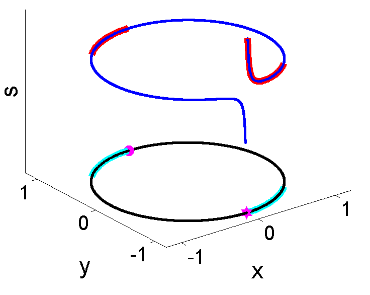
Figure 1: A plot of the two paths inside the curve ${\mathcal{J}}_{1}$, one of which diverges, and their projection into $J_{1}$ used to show that $P_{1}=(0,-1)$, the six-pointed star, is a smooth point of $J_{1}$.

Similarly, since $\deg J_{2}=3$, the membership test for $P_{2}$ with respect to $J_{2}$ requires tracking three paths on ${\mathcal{J}}_{2}$. The projection of the three paths limit to two distinct points on $J_{1}$ with the projection of two paths ending at $P_{2}$. Hence, the multiplicity of $P_{2}$ with respect to $J_{2}$ is $2$. Since $P_{2}\notin\pi({\mathcal{J}}_{2})$, the two paths in ${\mathcal{J}}_{2}$ whose projection limits to $P_{2}$ do not have an endpoint in ${\mathcal{J}}_{2}$.

1.3 Illustrative example using membership test

To demonstrate various formulations that we can utilize with Prop. 6, we consider computing the border rank of the cubic polynomial $x^{2}y$ in $\operatorname{{\rm Sym}}^{3}{\mathbb{C}}^{2}$, thereby verifying the results of [69, Table 1], namely $\operatorname{brk}(x^{2}y)=2$ (see also [93, 34, 17] for more general result). The computation also yields that either $\operatorname{rk}(x^{2}y)>2$ or $\operatorname{rk}(x^{2}y)=2$ with infinitely many decompositions. We will reconsider this example in Sections 1.4 and 1.5. This subsection ends with a general discussion of Waring problems.

Border rank 1 test using affine cones

We start our computation with the affine cone of the abstract join variety built from a parameterization:

$${\mathcal{J}}=\{(P,a)~{}|~{}P=v_{3}(a)\}\subset{\mathbb{C}}^{4}\times{\mathbb{C}}^{2}\hbox{~{}~{}where~{}~{}}v_{3}(a)=(a_{1}^{3},3a_{1}^{2}a_{2},3a_{1}a_{2}^{2},a_{2}^{3})$$

and $P=(P_{1},\ldots,P_{4})$. With $\pi(P,a)=P$, the affine cone of elements of $\operatorname{{\rm Sym}}^{3}{\mathbb{C}}^{2}$ of border rank $1$ is

$$J=\overline{\pi({\mathcal{J}})}=\overline{\{v_{3}(a)~{}|~{}a\in{\mathbb{C}}^{2}\}}\subset{\mathbb{C}}^{4}.$$

To compute $\dim J$, where $J$ is considered an affine variety in ${\mathbb{C}}^{4}$, we use (5) with $\dim{\mathcal{J}}=2$, $B=[I_{4}~{}0]$, and $f(P,a)=P-v_{3}(a)$. It is easy to verify that $\dim\operatorname{null}\left[\begin{array}[]{c}Jf(v_{3}(a^{*}),a^{*})\\ B\end{array}\right]=0$ for general $a^{*}\in{\mathbb{C}}^{2}$ thereby showing $\dim J=\dim{\mathcal{J}}=2$.

We construct a pseudowitness set for $J$, say $\{f,\pi,{\mathcal{M}},U\}$ where ${\mathcal{M}}$ is defined by

$$\left[\begin{array}[]{c}P_{1}-3P_{3}-5P_{4}-2\\ P_{2}+2P_{3}+4P_{4}-3\end{array}\right]=0\hbox{~{}~{}and~{}~{}}U=\left\{\begin{array}[]{l}(-0.754,3.29,-4.78,2.32,-0.91\omega^{k},1.32\omega^{k}),\\ (-6.01,7.99,-3.54,0.523,-1.82\omega^{k},0.806\omega^{k}),\\ (3.39,2.06,0.416,0.028,1.50\omega^{k},0.304\omega^{k})\end{array}\right\}$$

for $k=0,1,2$ where $\omega$ is the third root of unity. Hence, $\deg J=3$ meaning that we can test membership by tracking at most $3$ paths, say starting at $U^{\prime}\subset U$ obtained with $k=0$.

Since $x^{2}y$ corresponds to the point $P=(0,1,0,0)$, we consider the linear space ${\mathcal{L}}_{P}$ containing $P$ defined by the linear equations

$$\left[\begin{array}[]{c}P_{1}+(2+\sqrt{-1})P_{3}-3P_{4}\\ (P_{2}-1)+3P_{3}-(4+2\sqrt{-1})P_{4}\end{array}\right]=0.$$

The projection under $\pi$ of the endpoints of the three paths derived from deforming ${\mathcal{M}}$ to ${\mathcal{L}}_{p}$ are

$$\begin{array}[]{l}(0.181+0.284\sqrt{-1},0.120+0.313\sqrt{-1},0.054+0.330\sqrt{-1},-0.014+0.332\sqrt{-1}),\\ (-0.732+0.256\sqrt{-1},0.269+0.309\sqrt{-1},0.099-0.193\sqrt{-1},-0.114-0.010\sqrt{-1}),\\ (-0.400-0.149\sqrt{-1},0.138-0.233\sqrt{-1},0.129+0.112\sqrt{-1},-0.084+0.068\sqrt{-1}).\end{array}$$

Since $P$ is not one of these three points, we know $1<\operatorname{brk}(x^{2}y)\leq\operatorname{rk}(x^{2}y)$.

Border rank 2 test using affine cones

Every polynomial in $\operatorname{{\rm Sym}}^{3}{\mathbb{C}}^{2}$ has border rank at most $2$. We can verify this simply using (5) with

$${\mathcal{J}}=\{(P,a,b)~{}|~{}P=v_{3}(a)+v_{3}(b)\}\subset{\mathbb{C}}^{4}\times{\mathbb{C}}^{2}\times{\mathbb{C}}^{2}.$$ (6)

That is, for $\pi(P,a,b)=P$, we have that $J=\overline{\pi({\mathcal{J}})}={\mathbb{C}}^{4}$. Since $\operatorname{brk}(x^{2}y)>1$, this immediately shows that $\operatorname{brk}(x^{2}y)=2$ which we can verify by tracking one path defined by

$$P(t)=(1-t)(0,1,0,0)+t(-9\sqrt{-1},3-5\sqrt{-1},-1-11\sqrt{-1},-13)=v_{3}(a)+v_{3}(b).$$ (7)

At $t=1$, we can start with $a=(1+\sqrt{-1},1-2\sqrt{-1})$ and $b=(2-\sqrt{-1},1-\sqrt{-1})$. One clearly has $\lim_{t\rightarrow 0}P(t)=(0,1,0,0)$, but the corresponding $(a,b)$ diverge to infinity at $t\rightarrow 0$. Since starting from any of the possible decompositions of $P(1)$, namely

$$P(1)=v_{3}(\omega^{j}a)+v_{3}(\omega^{k}b)=v_{3}(\omega^{j}b)+v_{3}(\omega^{k}a)$$

where $j,k=0,1,2$ and $\omega$ is the third root of unity, yields a divergent path, Item 4 of Prop. 6 states that either $\operatorname{rk}(x^{2}y)>2$ or $\operatorname{rk}(x^{2}y)=2$ with infinitely many decompositions.

We will focus on distinguishing between these two cases in Sections 1.4 and 1.5.

Remark 9

Once (5) has been used to verify that a certain secant or join variety fill the ambient space, this technique of tracking only one path can be used in general as discussed in Section 4. Remarkably, it turns out that defective secant varieties are almost always those that one was expecting to fill the ambient space.

Border rank 2 test using affine coordinate patches

We compare the behavior of using affine cones above with the use of an affine coordinate patch with scalars. The advantage here is that, assuming sufficiently general coordinate patches, all paths will converge with this setup. The paths for which $\lim_{t\rightarrow 0}Z_{w}(t)$ does not exist in ${\mathcal{J}}$ have the corresponding scalar, namely $\lambda_{0}$, equal to zero. In particular, consider

$$Z=\left\{(P,\lambda,a,b)~{}\left|~{}\begin{array}[]{ll}P\lambda_{0}=v_{3}(a)\lambda_{1}+v_{3}(b)\lambda_{2}\\ r_{1}(P)=r_{2}(\lambda)=r_{3}(a)=r_{4}(b)=0\end{array}\right\}\right.\subset{\mathbb{C}}^{4}\times{\mathbb{C}}^{3}\times{\mathbb{C}}^{2}\times{\mathbb{C}}^{2}$$

where each $r_{i}$ is a general affine linear polynomial. The irreducible component of interest inside of $Z$ is $\overline{Z\setminus\mathcal{V}(\lambda_{0})}$. Since this irreducible set plays a similar role of the abstract join variety, we will call it ${\mathcal{J}}$. With projection $\pi(P,\lambda,a,b)=P$, we have that $\overline{\pi({\mathcal{J}})}=\mathcal{V}(r_{1}(P))$ which again verifies that every element in $\operatorname{{\rm Sym}}^{3}{\mathbb{C}}^{2}$ has border rank at most $2$.

For concreteness and simplicity, we take

$$r_{1}(P)=P_{2}-1,~{}~{}r_{2}(\lambda)=2\lambda_{0}-\lambda_{1}+3\lambda_{2}-1,~{}~{}r_{3}(a)=3a_{1}-2a_{2}-1,~{}~{}\hbox{and}~{}~{}r_{4}(b)=2b_{1}+3b_{2}-1.$$

Consider the path in $\overline{\pi({\mathcal{J}})}=\mathcal{V}(r_{1}(P))$ defined by $P(t)=(1-t)(0,1,0,0)+t(1+\sqrt{-1},1,2-\sqrt{-1},1-2\sqrt{-1})$. This path lifts to a path in ${\mathcal{J}}$, say, starting at $t=1$ with

$$\begin{array}[]{l}\lambda=(0.00145+0.000914\sqrt{-1},0.0482+0.0524\sqrt{-1},0.348+0.0169\sqrt{-1}),\\ a=(0.21+0.0532\sqrt{-1},-0.184+0.0797\sqrt{-1}),\hbox{~{}~{}and~{}~{}}\\ b=(0.157+0.0666\sqrt{-1},0.229-0.0444\sqrt{-1}).\end{array}$$

As mentioned above, the advantage is that this path is convergent, but the endpoint has $\lambda_{0}=0$ thereby showing that it would have diverged if we used an affine cone formulation.

Waring problem

This example of computing the rank and border rank of $x^{2}y$ in $\operatorname{{\rm Sym}}^{3}{\mathbb{C}}^{2}$ is an example of the so-called Waring problem, namely writing a homogeneous polynomial as a sum of powers of linear forms. We leave it as an open challenge problem to derive a general formula for the degrees of the corresponding secant varieties for these problems since this is equal to the maximum number of paths that need to be tracked in order to decide membership. We highlight some of the known partial results.

The Veronese variety that parameterizes $d^{\rm th}$ powers of linear forms in $n+1$ variables is classically known to have degree $d^{n}$.

In the binary case, the degree of $\sigma_{2}(X)$ where $X$ is the rational normal curve of degree $d$ parametrizing forms of type $(ax+by)^{d}$ is ${d-1\choose 2}$ [3, 77]. More generally in [40] it is shown that the variety parameterizing forms of type $(a_{0}x_{0}+\cdots+a_{n}x_{n})^{d}+(b_{0}x_{0}+\cdots+b_{n}x_{n})^{d}$ has degree

$$\frac{1}{2}\left(d^{2n}-\sum_{j=0}^{n}(-1)^{n-j}d^{j}{2n+1\choose j}{2n-j\choose j}\right).$$

The same paper also computes the degree of $\sigma_{2}(X)$ where $X$ is any Segre-Veronese variety which parameterizes multihomogeneous polynomials of type $L_{1}^{d_{1}}\cdots L_{k}^{d_{k}}$ where $L_{i}$ is a linear form in the variables $x_{0,i},\ldots,x_{n_{i},i}$ for $i=1,\ldots,k$. In this case, $\deg\sigma_{2}(X)$ is

$$\frac{1}{2}\left(\left((n_{1},\ldots,n_{k})!d_{1}^{n_{1}}\cdots d_{k}^{n_{k}}\right)^{2}-\sum_{l=0}^{n}{2n+1\choose l}(-1)^{n-l}\sum_{\sum j_{i}=n-l}(n_{1}-j_{1},\ldots,n_{k}-j_{k})!\prod_{i=1}^{k}{n_{i}+j_{i}\choose j_{j}}d_{i}^{n_{i}-j_{i}}\right).$$

The degree of some $k$-secants of ternary forms is known, e.g., [49, Thm. 1.4] and [62, Rem. 7.20].

1.4 Reduction to the curve case

Proposition 6 can determine membership in join varieties as well as provide some insight regarding membership in the constructible join. In particular, Item 5 of Prop. 6 shows that deciding membership in a join variety and the corresponding constructible join is equivalent when the join variety is a curve. The following describes one approach for deciding membership in the constructible join by reducing down to the curve case. Section 1.5 considers computing all decompositions of the form (1) and hence can also be used to decide membership in the constructible join by simply deciding if such a decomposition exists.

Suppose that ${\mathcal{J}}$ is the abstract join with corresponding join variety $J=\overline{\pi({\mathcal{J}})}$. Since we want to reduce down to the curve case, we will assume that $d:=\dim J>1$. Let $C$ be a general curve section of $J$, that is, $C=J\cap{\mathcal{L}}$ where ${\mathcal{L}}$ is a general linear space with $\operatorname{codim}{\mathcal{L}}=d-1$. Since $J$ is irreducible and ${\mathcal{L}}$ is general, the curve $C$ is also irreducible. Hence, ${\mathcal{J}}_{C}=\pi^{-1}(C)\cap{\mathcal{J}}$ is irreducible with $C=\overline{\pi({\mathcal{J}}_{C})}$. Therefore, one can use Item 5 of Prop. 6 to test membership in $C$ and $C^{0}=\pi({\mathcal{J}}_{C})$. However, since ${\mathcal{L}}$ is general, testing membership in $C^{0}$ and $C$ is typically not the problem of interest.

Given $[P]$, we want to decide if $[P]$ is a member of $J^{0}$ or $J$. Thus, we could modify the description above to replace ${\mathcal{L}}$ with ${\mathcal{L}}_{P}$, a general linear slice of codimension $d-1$ passing through $[P]$. If $C_{P}=J\cap{\mathcal{L}}_{P}$, then ${\mathcal{J}}_{C_{P}}=\pi^{-1}(C_{P})\cap{\mathcal{J}}$ need not be irreducible. However, since ${\mathcal{L}}_{P}$ is general through $[P]$, the closure of the images under $\pi$ of each irreducible component of ${\mathcal{J}}_{C_{P}}$ must either be the singleton $\{[P]\}$ or the curve $C_{P}$. Thus, one can apply Item 5 of Prop. 6 to each irreducible component of ${\mathcal{J}}_{C_{P}}$ whose image under $\pi$ is $C_{P}$.

The following illustrates this reduction to the curve case.

Example 10

Consider ${\mathcal{J}}$ as in (6) with $J=\overline{\pi({\mathcal{J}})}={\mathbb{C}}^{4}$ and $d=4$. Since a general curve section of $J$ is simply a general line in ${\mathbb{C}}^{4}$, we have $C={\mathcal{L}}$ where ${\mathcal{L}}\subset{\mathbb{C}}^{4}$ is a general line. It is easy to verify that ${\mathcal{J}}_{C}=\pi^{-1}(C)\cap{\mathcal{J}}$ is an irreducible curve of degree 30.

We now consider the point $P$ corresponding to $x^{2}y$, namely $(0,1,0,0)$. Hence, $C_{P}={\mathcal{L}}_{P}$ where ${\mathcal{L}}_{P}$ is a general line through this point. In this case, ${\mathcal{J}}_{C_{P}}=\pi^{-1}(C_{P})\cap{\mathcal{J}}$ is also an irreducible curve of degree 30. Hence, we can apply Item 5 of Prop. 6 to decide membership of $x^{2}y$ in $J^{0}=\pi({\mathcal{J}})$ by deciding membership in $C_{P}^{0}=\pi({\mathcal{J}}_{C_{P}})$. Since $C_{P}^{0}$ is a line, this is equivalent to tracking paths defined between a general point and $P$, as in (7). Since all paths diverge, Item 5 of Prop. 6 yields $\operatorname{rk}(x^{2}y)>2$.

For comparison, suppose that we want to consider $C_{Q}={\mathcal{L}}_{Q}$, which is a general line through $Q=(1,3,3,1)$ corresponding to $x^{3}+3\,x^{2}y+3\,xy^{2}+y^{3}$ which has rank one. The curve ${\mathcal{J}}_{C_{Q}}=\pi^{-1}(C_{Q})\cap{\mathcal{J}}$ is the union of two irreducible curves, say $V_{1}$ and $V_{2}$ with $\pi(V_{1})=\{Q\}$ and $\overline{\pi(V_{2})}=C_{Q}$, both of which yield decompositions.

1.5 Computing all decompositions

A fundamental question related to rank is to describe the set of all of decompositions of a point $[P]$. In numerical algebraic geometry, this means computing a numerical irreducible decomposition, i.e., a witness set for each irreducible component, of the fiber over $[P]$, namely

$${\mathcal{F}}_{P}:=\pi^{-1}([P])\cap{\mathcal{J}}(X_{1},\dots,X_{k}).$$

Computing ${\mathcal{F}}_{P}$ yields a membership test for $J^{0}(X_{1},\dots,X_{k})$ since $[P]\in J^{0}(X_{1},\dots,X_{k})$ if and only if ${\mathcal{F}}_{P}\neq\emptyset$. One approach is to directly compute a numerical irreducible decomposition using (1). Another approach is to perform a cascade [59, 86] starting with a witness set for ${\mathcal{J}}$. Since $\pi^{-1}([P])$ is defined by linear equations, computing ${\mathcal{F}}_{P}$ can be simply obtained by degenerating each general slicing hyperplane to a general hyperplane containing $\pi^{-1}([P])$. After each degeneration, the resulting points are either contained in $\pi^{-1}([P])$, forming witness point supersets, or not. The ones not contained in $\pi^{-1}([P])$ are used as the start points for the next degeneration. This process is described in detail in [60, § 2.2]. From the witness point supersets, standard methods in numerical algebraic geometry (e.g., see [14, Chap. 10]) are used to produce the numerical irreducible decomposition of ${\mathcal{F}}_{P}$.

After determining that $[P]\in J^{0}(X_{1},\dots,X_{k})$ by showing ${\mathcal{F}}_{P}\neq\emptyset$, a numerical irreducible decomposition of ${\mathcal{F}}_{P}$ can then be used to perform additional computations. One such computation is deciding if ${\mathcal{F}}_{P}$ contains real points, i.e., determining if there is a real decomposition, which is described in Section 3. Another application is to determine if there exist “simpler” decompositions of $[P]$, e.g., deciding if $[P]\in J^{0}(X_{1},\dots,X_{k-1})$. In the secant variety case, this is equivalent to deciding if the rank of $[P]$ is strictly less than $k$. The following illustrates this idea continuing with $x^{2}y$ considered in Section 1.3.

Example 11

With the setup from Section 1.3, consider computing all of the rank $3$ decompositions of $x^{2}y$ using affine cones. That is, we consider

$${\mathcal{J}}=\{(P,a,b,c)~{}|~{}P=v_{3}(a)+v_{3}(b)+v_{3}(c)\}\subset{\mathbb{C}}^{4}\times{\mathbb{C}}^{2}\times{\mathbb{C}}^{2}\times{\mathbb{C}}^{2}={\mathbb{C}}^{10}$$ (8)

which is irreducible of dimension 6 and degree 57. Thus, in a witness set for ${\mathcal{J}}$, we have a general linear space ${\mathcal{L}}$ of codimension 6 defined by linear polynomials $\ell_{i}(P,a,b,c)=0$, $i=1,\dots,6$ and a witness point set $W={\mathcal{J}}\cap{\mathcal{L}}$ consisting of 57 points.

For $i=1,\dots,4$, let $m_{i}(P)$ be a general linear polynomial which vanishes at $(0,1,0,0)$. The cascade simply replaces the condition $\ell_{i}=0$ with $m_{i}=0$ sequentially for $i=1,\dots,4$. For $i=1,2,3$, we have that ${\mathcal{J}}\cap\mathcal{V}(m_{1},\dots,m_{i},\ell_{i+1},\dots,\ell_{6})$ consists of 57 points, none of which are not contained in ${\mathcal{F}}_{P}$. However, ${\mathcal{J}}\cap\mathcal{V}(m_{1},\dots,m_{4},\ell_{5},\ell_{6})$ consists of 45 points, all of which are contained in ${\mathcal{F}}_{P}$. Hence, ${\mathcal{F}}_{P}\neq\emptyset$ thereby showing that $\operatorname{rk}(x^{2}y)\leq 3$. In fact, these 45 points form a witness point set for ${\mathcal{F}}_{P}$, which is an irreducible surface of degree $45$.

Even though Ex. 10 shows that $\operatorname{rk}(x^{2}y)>2$, we can verify this by showing that ${\mathcal{F}}_{P}\cap\mathcal{V}(c)=\emptyset$ using the witness point set for ${\mathcal{F}}_{P}$ computed above. To that end, let $r_{i}(c)$ for $i=1,2$ be a general linear polynomial vanishing at $c=0$. By deforming from the general linear $\ell_{5}(P,a,b,c)$ to $r_{1}(c)$, we obtain that ${\mathcal{J}}\cap\mathcal{V}(m_{1},\dots,m_{4},r_{1},\ell_{6})$ consists of 36 points, none of which satisfy $c=0$. We then deform $\ell_{6}$ to $r_{2}$ thereby computing ${\mathcal{J}}\cap\mathcal{V}(m_{1},\dots,m_{4},r_{1},r_{2})$, which is empty. Hence, ${\mathcal{F}}_{P}\cap\mathcal{V}(c)=\emptyset$ so that $\operatorname{rk}(x^{2}y)>2$.

2 Boundary

By using the various approaches described in Section 1, one is able to use numerical algebraic geometry to determine membership in both the constructible join $J^{0}(X_{1},\dots,X_{k})$ and the join variety $J(X_{1},\dots,X_{k})$. An interesting object is the boundary $\partial:=\overline{J(X_{1},\dots,X_{k})\setminus J^{0}(X_{1},\dots,X_{k})}$ which is the closure of the elements which arose by closing the constructible set $J^{0}(X_{1},\dots,X_{k})$. As a subset of $J(X_{1},\dots,X_{k})$, the boundary $\partial$ may consist of irreducible components of various codimension. In the following, we describe an approach for computing the irreducible components of $\partial$ which have codimension one with respect to $J(X_{1},\dots,X_{k})$, denoted $\partial_{1}$, derived from [57, § 3].

Following with the numerical algebraic geometric framework, we aim to compute a pseudowitness set for $\partial_{1}$. To do this, we first consider the case where ${\mathcal{C}}\subset{\mathbb{P}}^{N}\times{\mathbb{C}}^{M}$ is an irreducible curve and the projection $\pi([P],X)=[P]$ is generically finite-to-one on ${\mathcal{C}}$, i.e., $\dim{\mathcal{C}}=1$ and $\dim_{gf}({\mathcal{C}},\pi)=0$. The boundary of $C=\pi({\mathcal{C}})$ consists of at most finitely many points $\partial_{C}=\overline{C}\setminus C$.

Example 12

Consider the irreducible curve ${\mathcal{C}}=\{([a,b],x)~{}|~{}a\cdot x=b\}\subset{\mathbb{P}}^{1}\times{\mathbb{C}}$ and $\pi([a,b],x)=[a,b]$. Generically, $\pi$ is a one-to-one map from ${\mathcal{C}}$ to ${\mathbb{P}}^{1}$. Since we have $x=b/a\in{\mathbb{C}}$ when $a\neq 0$, one can easily verify that the boundary of $C=\pi({\mathcal{C}})$ is $\partial_{C}=\{[0,1]\}\subset{\mathbb{P}}^{1}$.

The first task in computing $\partial_{C}$ is to compute a superset of $\partial_{C}$ consisting of finitely many points. To that end, consider the closure of ${\mathcal{C}}\subset{\mathbb{P}}^{N}\times{\mathbb{C}}^{M}$ in ${\mathbb{P}}^{N}\times{\mathbb{P}}^{M}$, say $\overline{\mathcal{C}}$. Then, a finite superset of $\partial_{C}$ is the set of points in $\overline{C}$ whose fiber intersects “infinity.” That is, if we have coordinates $x\in{\mathbb{C}}^{M}$ and $[y]\in{\mathbb{P}}^{M}$ with the embedding given by

$$(x_{1},\dots,x_{M})\in{\mathbb{C}}^{M}\mapsto[1,x_{1},\dots,x_{M}]\in{\mathbb{P}}^{M},$$

then a finite superset of $\partial_{C}$ is $\pi(\overline{\mathcal{C}}\cap\mathcal{V}(y_{0}))$.

Example 13

Continuing with the setup from Ex. 12, one can verify that

$$\overline{\mathcal{C}}=\{([a,b],[y_{0},y_{1}])~{}|~{}a\cdot y_{1}=b\cdot y_{0}\}\subset{\mathbb{P}}^{1}\times{\mathbb{P}}^{1}\hbox{~{}~{}and~{}~{}}\pi(\overline{\mathcal{C}}\cap\mathcal{V}(y_{0}))=\{[0,1]\}.$$

In Ex. 13, it was the case that $\partial_{C}=\pi(\overline{\mathcal{C}}\cap\mathcal{V}(y_{0}))$. However, since $\partial_{C}\subset\pi(\overline{\mathcal{C}}\cap\mathcal{V}(y_{0}))$ in general, we must investigate each point in $\pi(\overline{\mathcal{C}}\cap\mathcal{V}(y_{0}))$ via Sections 1.4 and 1.5 to determine if it is contained in $\partial_{C}$.

With the special case in hand, we now turn to the general case of ${\mathcal{J}}$ as in (3). Let $J$ and $J^{0}$ be the corresponding join variety and constructible join, i.e., $J=\overline{\pi({\mathcal{J}})}$ and $J^{0}=\pi({\mathcal{J}})$, and $d=\dim J$. Since the case $d=0$ is trivial, we will assume $d\geq 1$. Since we aim to compute witness points sets for the codimension 1 components, $\partial_{1}$, of the boundary $\partial=\overline{J\setminus J^{0}}$, i.e., $\partial_{1}$ has pure-dimension $d-1$, we can restrict our attention to a general curve section of $J$, say $C$. This restriction cuts $\partial_{1}$ down to finitely many points, i.e., a witness point set for $\partial_{1}$, which we aim to compute.

Since $C$ is a general curve section, ${\mathcal{M}}=\pi^{-1}(C)\cap{\mathcal{J}}$ is irreducible. Finally, we take a general curve section of ${\mathcal{M}}$, say ${\mathcal{C}}$. Thus, ${\mathcal{C}}$ is an irreducible curve with $\overline{\pi({\mathcal{C}})}=C$ and $\dim_{gf}({\mathcal{C}},\pi)=0$. Applying the procedure described above yields a finite set of points containing $\partial_{C}$. Since the restriction from ${\mathcal{M}}$ to a general curve section ${\mathcal{C}}$ may have introduced new points in the boundary, we simply need to investigate each point with respect to ${\mathcal{M}}$ rather than ${\mathcal{C}}$ via Sections 1.4 and 1.5. In the end, we obtain the finitely many points forming a witness point set for $\partial_{1}$.

Example 14

As with Section 1.3, we use a parameterization to compute the codimension one component of the boundary, $\partial$, in $\operatorname{{\rm Sym}}^{3}{\mathbb{C}}^{2}$ of border rank $2$. Since every polynomial in $\operatorname{{\rm Sym}}^{3}{\mathbb{C}}^{2}$ has border rank $2$, the codimension one component of $\partial$ is a hypersurface: the tangential variety of the rational normal cubic curve.

Since $J=\operatorname{{\rm Sym}}^{3}{\mathbb{C}}^{2}$, a general curve section $C$ of $J$ is simply a general line. Following an affine cone formulation as in (6), we take, for exposition, $C$ defined by the equations

$$P_{1}+3P_{4}-2=P_{2}-4P_{4}+3=P_{3}-2P_{4}-4=0.$$

Since $\dim_{gf}({\mathcal{J}},\pi)=0$, we have ${\mathcal{C}}={\mathcal{M}}=\pi^{-1}(C)\cap{\mathcal{J}}$ is the curve

$${\mathcal{C}}=\{(P,a,b)~{}|~{}P=v_{3}(a)+v_{3}(b)\in C\}\subset{\mathbb{C}}^{4}\times{\mathbb{C}}^{2}\times{\mathbb{C}}^{2}.$$

Next, we compute the closure, $\overline{\mathcal{C}}$, of ${\mathcal{C}}$ in ${\mathbb{C}}^{4}\times{\mathbb{P}}^{4}$ where ${\mathbb{C}}^{2}\times{\mathbb{C}}^{2}\hookrightarrow{\mathbb{P}}^{4}$ given by

$$(a,b)\in{\mathbb{C}}^{2}\times{\mathbb{C}}^{2}\mapsto[1,a_{1},a_{2},b_{1},b_{2}]\in{\mathbb{P}}^{4}.$$

With coordinates $[y_{0},\dots,y_{4}]\in{\mathbb{P}}^{4}$, we find that $\pi(\overline{\mathcal{C}}\cap\mathcal{V}(y_{0}))$ consists of the following four points:

$$\begin{array}[]{ll}(2.308,-3.410,3.794,-0.103),&(-35.743,47.325,29.163,12.581),\\ (4.328,-6.103,2.448,-0.776),&(0.018,-0.357,5.321,0.661).\end{array}$$

Finally, we verified that each of these points corresponds to an element that has rank larger than $2$ via Sections 1.4 and 1.5. Hence, the codimension one component of $\partial$, namely $\partial_{1}$, is a degree $4$ hypersurface.

Although we can use numerical algebraic geometry to test membership in this hypersurface via Section 1, we can also easily recover the defining equation exactly in this case using [12]:

$$P_{1}^{2}P_{4}^{2}-6P_{1}P_{2}P_{3}P_{4}+4P_{1}P_{3}^{3}+4P_{2}^{3}P_{4}-3P_{2}^{2}P_{3}^{2}=0.$$

Clearly, $(0,1,0,0)$, corresponding to $x^{2}y$, lies on this hypersurface.

3 Real decompositions

For a real $[P]$, i.e., the line $[P]$ is defined by linear polynomials with real coefficients, a natural question is to determine if real decompositions exist after computing the fiber ${\mathcal{F}}_{P}$ as in Section 1.5 showing that decompositions over the complex numbers exist. With a witness set for each irreducible component of ${\mathcal{F}}_{P}$, where all general choices involve selecting real numbers, the homotopy-based approach of [51] (see also [95]) can be used to determine if the irreducible component contains real points. The techniques described in [51, 95] rely upon computing critical points of the distance function as proposed by Seidenberg [82] (see also [7, 47, 79]). For secant varieties, this yields a method to determine the real rank of a real element.

Let $F$ be a system of $n$ polynomials in $N$ variables with real coefficients and $V\subset\mathcal{V}(F)\subset{\mathbb{C}}^{N}$ be an irreducible component. Fix a real point $x^{*}\in{\mathbb{R}}^{N}$ such that $x^{*}\notin\mathcal{V}(F)$ sufficiently general. Following Seidenberg [82], we consider the optimization problem

$$\min\{\|x-x^{*}\|_{2}^{2}~{}|~{}x\in V\cap{\mathbb{R}}^{N}\}.$$ (9)

Every connected component $C$ of $V\cap{\mathbb{R}}^{N}$ has a global minimizer of the distance functions from $x^{*}$ to $C$, i.e., there exists $x\in C$ such that $\|x-x^{*}\|_{2}^{2}\leq\|z-x^{*}\|_{2}^{2}$ for every $z\in C$. Thus, there exists $\lambda\in{\mathbb{P}}^{n}$ with

$$G(x,\lambda)=\left[\begin{array}[]{c}F(x)\\ \lambda_{0}(x-x^{*})+\sum_{i=1}^{n}\lambda_{i}{\nabla}F_{i}(x)\end{array}\right]=0$$ (10)

where ${\nabla}F_{i}$ is the gradient of $F_{i}$. For the projection map $\pi(x,\lambda)=x$, the set $\pi(\mathcal{V}(G))\subset{\mathbb{C}}^{N}$ is called the set of critical points of (9) and it intersects every connected component of $V\cap{\mathbb{R}}^{N}$. Hence, $V\cap{\mathbb{R}}^{N}=\emptyset$ if and only if there are no real critical points for (9).

This method allows one to decide if a real decomposition exists by deciding if there exists a real critical point of the distance function. As a by-product, one obtains the closest decomposition to the given point. When the set of critical points may be positive-dimensional, the approach presented in [51] uses a homotopy-based approach to reduce down to testing the reality of finitely many critical points. Therefore, the problem of deciding if a real decomposition exists can be answered by deciding the reality of finitely many points.

Example 15

Consider deciding if the real rank of $x^{2}y$ in $\operatorname{{\rm Sym}}^{3}{\mathbb{C}}^{2}$ is the same as the complex rank, namely $3$. In Ex. 11, we computed ${\mathcal{F}}_{P}$, which is irreducible of dimension $2$ and degree $45$. In particular, we can take

$$F(a,b,c)=\left[\begin{array}[]{c}a_{1}^{3}+b_{1}^{3}+c_{1}^{3}\\ 3(a_{1}^{2}a_{2}+b_{1}^{2}b_{2}+c_{1}^{2}c_{2})-1\\ 3(a_{1}a_{2}^{2}+b_{1}b_{2}^{2}+c_{1}c_{2}^{2})\\ a_{2}^{3}+b_{2}^{3}+c_{2}^{3}\end{array}\right].$$

We aim to compute the critical points of the distance from

$$\alpha=(1,2),~{}~{}\beta=(-2,1),~{}~{}\gamma=(1,-1)$$ (11)

which arise from the solutions $(a,b,c)\in{\mathbb{C}}^{6}$ and $\delta\in{\mathbb{P}}^{4}$ of

$$G(a,b,c,\delta)=\left[\begin{array}[]{c}F(a,b,c)\\ \delta_{0}(a-\alpha,b-\beta,c-\gamma)+\sum_{i=1}^{4}\delta_{i}{\nabla}F_{i}(a,b,c)\end{array}\right].$$

Solving $G=0$ yields 234 critical points, of which 8 are real. Hence, the real rank of $x^{2}y$ is indeed $3$ (cfr. [27]) where the one of minimal distance from $(\alpha,\beta,\gamma)$ is the decomposition (to three digits)

$$x^{2}y=(0.721x+0.2849y)^{3}+(-1.429x+1.101y)^{3}+(1.365x-1.107y)^{3}.$$ (12)

Since minimizing the distance to a nongeneric point can yield potential issues, one should treat the center point $x^{*}$ as a parameter and utilize a parameter homotopy (e.g., see [14, Chap. 6]). The number of such paths to track with this setup is called the Euclidean distance degree [47].

Example 16

Consider solving the following optimizaton problem

$$\min\{x^{2}+(y+2)^{2}~{}|~{}(x,y)\in\overline{\pi({\mathcal{J}}_{1})}\cap{\mathbb{R}}^{2}\}$$

where ${\mathcal{J}}_{1}$ and $\pi$ as in Ex. 8. Since $\overline{\pi({\mathcal{J}}_{1})}=\mathcal{V}(x^{2}+y^{2}-1)$, it is clear that the two critical points are $(0,\pm 1)$ with $(0,-1)\notin\pi({\mathcal{J}}_{1})$. Thus, we consider this as a member of the family of optimization problems

$$\min\{(x-q_{1})^{2}+(y-q_{2})^{2}~{}|~{}(x,y)\in\overline{\pi({\mathcal{J}}_{1})}\cap{\mathbb{R}}^{2}\}$$

parameterized by $q$. The critical points are obtained by solving

$$\left[\begin{array}[]{c}x(1+s^{2})-2s\\ y(1+s^{2})-(1-s^{2})\\ \lambda_{0}\left[\begin{array}[]{c}x-q_{1}\\ y-q_{2}\\ 0\end{array}\right]+\lambda_{1}\left[\begin{array}[]{c}1+s^{2}\\ 0\\ 2sx-2\end{array}\right]+\lambda_{2}\left[\begin{array}[]{c}0\\ 1+s^{2}\\ 2sy+2s\end{array}\right]\end{array}\right]=0$$

which, for a general $q\in{\mathbb{C}}^{2}$, has two solutions. A parameter homotopy that deforms the parameters from the selected value of $q$ to $(0,-2)$ yields solution two paths. As paths in ${\mathbb{C}}^{3}\times{\mathbb{P}}^{2}$, only one of these two paths has a limit point since $(0,-1)\notin\pi({\mathcal{J}}_{1})$. However, since we are interested in $\overline{\pi({\mathcal{J}}_{1})}$, we only need to observe the limit of the projection of these two paths in $(x,y)\in{\mathbb{C}}^{2}$, which yields the two critical points $(0,\pm 1)$.

The computation of all critical points provides a global approach for deciding if a real decomposition exists. Such a global approach may be computationally expensive when the number of critical points is large. Thus, we also describe a local approach based on gradient descent homotopies [50] with the aim of computing a real critical point. Although there is no guarantee, such a local approach can provide a quick affirmation that a real decomposition exists.

With the setup as above, we consider the gradient descent homotopy

$$H(z,\delta,t)=\left[\begin{array}[]{c}F(z)-t\cdot F(x^{*})\\ \delta_{0}(z-x^{*})+\sum_{i=1}^{n}\delta_{i}{\nabla}F_{i}(z)\end{array}\right]=0.$$

Clearly, $H(x,\lambda,0)=G(x,\lambda)=0$ for $G$ as in (10). We consider the homotopy path $(z(t),\delta(t))$ where $z(1)=x^{*}\in{\mathbb{R}}^{N}$ and $\delta(1)=[1,0,\dots,0]\in{\mathbb{P}}^{n}$. If this homotopy path is smooth for $0<t\leq 1$ and converges as $t\rightarrow 0$, then $z(0)$ is a real critical point with respect to $F$. We note that $H$ is a so-called Newton homotopy since $\partial H/\partial t$ is independent of $z$ and $\delta$. Newton homotopies will also be used below in Section 4.

One can quickly try gradient descent homotopies for various $x^{*}\in{\mathbb{R}}^{N}$ with the goal of computing a real critical point, provided one exists.

Example 17

With the setup from Ex. 15 and (11), we consider the gradient descent homotopy

$$H(a,b,c,\delta,t)=\left[\begin{array}[]{c}F(a,b,c)-t\cdot F(\alpha,\beta,\gamma)\\ \delta_{0}(a-\alpha,b-\beta,c-\gamma)+\sum_{i=1}^{4}\delta_{i}\cdot\nabla F_{i}(a,b,c)\end{array}\right].$$

The path, which starts at $t=1$ with $(\alpha,\beta,\gamma,[1,0,\dots,0])$ yields a smooth and convergent path with the endpoint corresponding the decomposition of minimal distance from $(\alpha,\beta,\gamma)$ in (12).

4 Generic cases

When the join variety $J(X_{1},\dots,X_{k})$ fills the ambient projective space, the degree of the join variety is $1$. In this section, we modify the approach presented in Prop. 6 to use a Newton homotopy which can compute a decomposition of a generic tensor by tracking one path. Such paths can even be tracked certifiably [52, 54].

Let $[P]\in J(X_{1},\dots,X_{k})$ be generic. Thus, the dimension and degree of the fiber over $[P]$ is the same over a nonempty Zariski open subset of $J(X_{1},\dots,X_{k})$, i.e.,

$$d:=\dim_{gf}({\mathcal{J}},\pi)=\dim\pi^{-1}([P])\cap{\mathcal{J}}\hbox{~{}~{}and~{}~{}}\deg_{gf}(J,\pi)=\deg\pi^{-1}([P])\cap{\mathcal{J}}.$$

The first step for computing a decomposition of $[P]$ is to produce a starting point. This is performed by selecting generic $x_{i}^{*}\in{\mathcal{C}}(X_{i})$ and computing $P^{*}=\sum_{i=1}^{k}x_{i}^{*}$. That is, $([P^{*}],x_{1}^{*},\dots,x_{k}^{*})\in{\mathcal{J}}$ is sufficiently generic with respect to ${\mathcal{J}}$ and $[P]$.

With this setup, consider the homotopy that deforms the fiber as we move along the straight line from $[P^{*}]$ to $[P]$, namely $\pi^{-1}(t[P^{*}]+(1-t)[P])\cap{\mathcal{J}}$. If $d>0$, i.e., the fiber is positive-dimensional, we can reduce down to tracking along a path by simply intersecting with a generic linear space ${\mathcal{L}}$ of codimension $d$ passing through the point $([P^{*}],x_{1}^{*},\dots,x_{k}^{*})$. This results in the Newton homotopy

$$\pi^{-1}(t[P^{*}]+(1-t)[P])\cap{\mathcal{J}}\cap{\mathcal{L}}$$

where, at $t=1$, we have start point $(x_{1}^{*},\dots,x_{k}^{*})$. The endpoint of this path yields a decomposition of $[P]$ in the form (1).

4.1 Illustrative example

We demonstrate decomposing a general element via tracking one path on cubic forms in $3$ variables. For a cubic form $C(x)$, we aim to write it as

$$C(x)=Q(x)\cdot L_{1}(x)+L_{2}(x)^{3}$$ (13)

where $Q(x)=q_{0}x_{0}^{2}+q_{1}x_{0}x_{1}+\cdots+q_{5}x_{2}^{2}$ is a quadratic form and $L_{i}(x)=x_{0}+a_{i1}x_{1}+a_{i2}x_{2}$ is a linear form with $q_{k},a_{ij}\in{\mathbb{C}}$. Geometrically, this means $C(x)\in J(\mathcal{O}^{2}(\nu_{3}(\mathbb{P}^{2})),\nu_{3}(\mathbb{P}^{2}))$ where $\mathcal{O}^{2}(\nu_{3}(\mathbb{P}^{2}))$ is the second osculating variety to the Veronese surface $\nu_{3}(\mathbb{P}^{2})$. By (5), it is easy to verify that a general cubic $C(x)$ must have finitely many decompositions of the form (13). We will compute decompositions of

$$C_{1}(x)=x_{0}^{3}+x_{1}^{3}+x_{2}^{3}\hbox{~{}~{}~{}~{}and~{}~{}~{}~{}}C_{2}(x)=4x_{0}^{2}x_{2}+x_{1}^{2}x_{2}-8x_{0}^{3}$$

where the cubic $C_{2}$ defines a curve called the “witch of Agnesi.” Starting with

$$\begin{array}[]{rcl}C^{*}(x)&=&\left(x_{0}^{2}+(1+\sqrt{-1})x_{0}x_{1}+3x_{0}x_{2}-2x_{1}^{2}+(3-\sqrt{-1})x_{1}x_{2}+2x_{2}^{2}\right)(x_{0}+2x_{1}+3x_{2})\\ &&~{}~{}~{}~{}+~{}\left(x_{0}-(3+\sqrt{-1})x_{1}+5x_{2}\right)^{3},\end{array}$$

the Newton homotopy deforming from $C^{*}$ to $C_{i}$ which is obtained by taking coefficients of

$$tC^{*}(x)+(1-t)C_{i}(x)=(q_{0}x_{0}^{2}+q_{1}x_{0}x_{1}+\cdots+q_{5}x_{2}^{2})(x_{0}+a_{11}x_{1}+a_{12}x_{2})+(x_{0}+a_{21}x_{1}+a_{22}x_{2})^{3}$$

yields the following decompositions, which we have converted to exact representation using [12]:

$$\begin{array}[]{rcl}C_{1}(x)&=&(-3x_{0}x_{1}+3(1-\sqrt{-3})x_{0}x_{2}/2-3x_{1}^{2}+3(1-\sqrt{-3})x_{1}x_{2}/2)(x_{0}-(1-\sqrt{-3})x_{2}/2)\\ &&~{}~{}~{}~{}+~{}(x_{0}+x_{1}-(1-\sqrt{-3})x_{2}/2)^{3},\vskip 6.0pt plus 2.0pt minus 2.0pt\\ C_{2}(x)&=&(-9x_{0}^{2}-9x_{1}^{2}/4)(x_{0}-\sqrt{3}x_{1}/6-4x_{2}/9)+(x_{0}-\sqrt{3}x_{1}/2)^{3}.\\ \end{array}$$

4.2 Projections and Newton homotopies

When the join variety does not fill the ambient space, we will modify our approach by combining Newton homotopies, projections, and local numerical solving techniques, e.g., [65, 85]. This yields a local method which can be used to show upper bounds on rank and border rank over ${\mathbb{C}}$ and ${\mathbb{R}}$.

If $c:=\operatorname{codim}J(X_{1},\dots,X_{k})>0$, let $\psi$ be a linear map such that $\overline{\psi(J(X_{1},\dots,X_{k}))}$ fills the ambient space and $\dim_{gf}(J(X_{1},\dots,X_{k}),\psi)=0$. We could apply the method above to attempt to decompose $\psi([P])$ using a Newton homotopy in $\overline{\psi(J(X_{1},\dots,X_{k}))}$ starting from a randomly selected point. Since the fiber $\psi^{-1}(\psi([P]))\cap J(X_{1},\dots,X_{k})$ may contain many other elements in addition to $[P]$, we may need to run the Newton homotopy approach with many starting points to increase our chances of ending at a decomposition of $[P]$.

Another approach is to use [56] to compute all of the elements in a fiber over a general element $\psi([P^{*}])$ and then use the Newton homotopy to track all of the corresponding paths as $\psi([P^{*}])$ is deformed to $\psi([P])$. If $\psi$ was generic with respect to $[P]$ so that the fiber $\psi^{-1}(\psi([P]))\cap J(X_{1},\dots,X_{k})$ is zero dimensional, then tracking all of these paths and observing in any end at $[P]$ is equivalent to Item 1 of Prop. 6.

Rather than utilizing a global method, we will use local numerical decomposition methods, e.g., see [65, 85], to “seed” our Newton homotopy. Such local methods generally use optimization techniques to numerically approximate a decomposition, and these approximations typically provide excellent starting points. Moreover, if the homotopy is defined by polynomials with real coefficients and the start point is real, then the endpoint is also real provided that the path is smooth on $(0,1]$. This observation allows one to yield upper bounds on the real rank and border rank by demonstrating the existence of real paths.

Example 18

Reconsider ${\mathcal{J}}_{1}$ from Ex. 8 where $J_{1}:=\overline{\pi({\mathcal{J}}_{1})}=\mathcal{V}(x^{2}+y^{2}-1)\subset{\mathbb{C}}^{2}$. For the projection map $\psi(x,y)=2x+3y$, it is easy to verify that $\overline{\psi(J_{1})}={\mathbb{C}}$ with $\dim_{gf}(J_{1},\psi)=0$ and $\deg_{gf}(J_{1},\psi)=2$. We aim to show that there is a real path $(x(t),y(t),s(t))\in{\mathcal{J}}_{1}$ such that $\lim_{t\rightarrow 0}\pi(x(t),y(t))=(0,-1)$.

For this simple example, we can easily construct a point nearby $(0,-1)$ which has a real point in its fiber, say $(x^{*},y^{*},s^{*})=(20/101,-99/101,10)\in{\mathcal{J}}_{1}$, which we take as the start point for the Newton homotopy

$$H(x,y,s,t)=\left[\begin{array}[]{c}x(1+s^{2})-2s\\ y(1+s^{2})-(1-s^{2})\\ \psi(x,y)-(t\cdot\psi(x^{*},y^{*})+(1-t)\cdot\psi(0,-1))\end{array}\right].$$

One can easily observe that the path $(x(t),y(t),s(t))$ with $(x(1),y(1),s(1))=(x^{*},y^{*},s^{*})$ is smooth on $(0,1]$ with $(x(t),y(t))\rightarrow(0,-1)$ as $t\rightarrow 0$. Since $(0,-1)\notin\pi({\mathcal{J}}_{1})$, this path must diverge in ${\mathcal{J}}_{1}$.

For numerical computations, it can be easier to track convergent paths. In this case, one can compactify the fiber with respect to $\pi$ to yield

$$H(x,y,s,t)=\left[\begin{array}[]{c}x(s_{0}^{2}+s_{1}^{2})-2s_{0}s_{1}\\ y(s_{0}^{2}+s_{1}^{2})-(s_{0}^{2}-s_{1}^{2})\\ \psi(x,y)-(t\cdot\psi(x^{*},y^{*})+(1-t)\cdot\psi(0,-1))\end{array}\right]$$

with start point $x=x^{*}$, $y=y^{*}$, and $s=[1,s^{*}]$ at $t=1$. Thus, one is actually tracking the path on the closure of ${\mathcal{J}}_{1}$ in ${\mathbb{C}}^{2}\times{\mathbb{P}}^{1}$. The endpoint of this smooth path on $(0,1]$ is $(x,y)=(0,-1)$ with $s=[0,1]$.

5 Examples

The previous sections have described various approaches for computing information about join and secant varieties along with several illustrative examples. In this section, we present several larger examples which were computed using the methods described above with computations facilitated by Bertini [13, 14].

5.1 Complex multiplication tensor

Complex multiplication can be treated as a bilinear map from ${\mathbb{R}}^{2}\times{\mathbb{R}}^{2}\rightarrow{\mathbb{R}}^{2}$, namely

$$(a,b)\cdot(c,d)\mapsto(ac-bd,ad+bc),$$

which, using the definition, involves $4$ multiplications. Treating this as a bilinear map from ${\mathbb{C}}^{2}\times{\mathbb{C}}^{2}\rightarrow{\mathbb{C}}^{2}$, we will use the above approaches to compute the rank and border rank (over ${\mathbb{C}}$) of this bilinear map, both of which are $2$. We will then demonstrate how our method shows that the real rank of this bilinear map is $3$. In particular, the decomposition by Gauss, namely

$$ac-bd=(a+b)\cdot c-b\cdot(c+d),~{}~{}~{}~{}ad+bc=(a+b)\cdot c+a\cdot(d-c),$$ (14)

shows that the real rank is at most $3$ via the three multiplications $(a+b)\cdot c$, $b\cdot(c+d)$, and $a\cdot(d-c)$.

Over the complex numbers

Let $T:{\mathbb{C}}^{2}\times{\mathbb{C}}^{2}\rightarrow{\mathbb{C}}^{2}$ denote the complex multiplication bilinear map. We first aim to compute $\operatorname{brk}T$ and $\operatorname{rk}T$. Observe that $T\in{\mathbb{C}}^{2}\otimes{\mathbb{C}}^{2}\otimes{\mathbb{C}}^{2}$ with its rank and border rank corresponding to computing minimal decompositions with respect to the Segre variety

$$S:=Seg({\mathbb{P}}^{1}\times{\mathbb{P}}^{1}\times{\mathbb{P}}^{1})\subset{\mathbb{P}}({\mathbb{C}}^{2}\otimes{\mathbb{C}}^{2}\otimes{\mathbb{C}}^{2})={\mathbb{P}}({\mathbb{C}}^{8}).$$

To accomplish this, we compute a pseudowitness set for $S=\sigma_{1}(S)\subset{\mathbb{P}}({\mathbb{C}}^{8})$ for which $\deg\sigma_{1}(S)=6$. The membership test described in Prop. 6 tracked $6$ paths and found that each path converged to some finite endpoint which does not correspond to $T$. Therefore, $\operatorname{rk}T\geq\operatorname{brk}T>1$.

Next, we turn our attention to $\sigma_{2}(S)$, which fills the whole space. Hence, we know $\operatorname{brk}T=2$. We use the method from Section 4 to track one solution path which indeed converges to a decomposition of $T$ thereby showing $[T]\in\sigma_{2}^{0}(S)\subset\sigma_{2}(S)$, i.e., $\operatorname{rk}T=\operatorname{brk}T=2$.

For example, if we look for decompositions of the form

$$\begin{bmatrix}ac-bd\\ ad+bc\end{bmatrix}=\begin{bmatrix}x_{11}&x_{12}\\ x_{21}&x_{22}\end{bmatrix}\begin{bmatrix}(a+y_{12}b)\cdot(c+z_{12}d)\\ (y_{21}a+b)\cdot(z_{21}c+d)\end{bmatrix},$$ (15)

then our setup tracking one path yielded the decomposition

$$\begin{array}[]{rcl}ac-bd&=&~{}\left((a-ib)\cdot(c-id)-(b-ia)\cdot(d-ic)\right)/2\\ ad+bc&=&i\left((a-ib)\cdot(c-id)+(b-ia)\cdot(d-ic)\right)/2\end{array}$$

where $i=\sqrt{-1}$ with the two multiplication being $(a-ib)\cdot(c-id)$ and $(b-ia)\cdot(d-ic)$.

Over the real numbers

Since (14) shows that $\operatorname{rk}_{\mathbb{R}}T\leq 3$, we know that $\operatorname{rk}_{\mathbb{R}}T=3$ if and only if $\operatorname{rk}_{\mathbb{R}}T>2$. In (15), we used a specialized form to compute a decomposition over ${\mathbb{C}}$. In this case, there were only finitely many decompositions and all were not real.

We could also work with a fully general formulation:

$$\begin{bmatrix}ac-bd\\ ad+bc\end{bmatrix}=\begin{bmatrix}x_{11}&x_{12}\\ x_{21}&x_{22}\end{bmatrix}\begin{bmatrix}(y_{11}a+y_{12}b)\cdot(z_{11}c+z_{12}d)\\ (y_{21}a+y_{22}b)\cdot(z_{21}c+z_{22}d)\end{bmatrix}$$

which, by taking coefficients, defines a variety $V\subset{\mathbb{C}}^{12}$, the union of two irreducible varieties $V_{1}$ and $V_{2}$, each having dimension $4$ and degree $9$. Using two different approaches, we show that $V\cap{\mathbb{R}}^{12}=\emptyset$.

First, using the setup from Section 3, we compute the critical points of the distance between $V$ and a random point in $[-1,1]^{12}$. Since this yields $18$ critical points, all of which are nonreal, we know $\operatorname{rk}_{\mathbb{R}}T>2$.

Alternatively, since the two irreducible components of $V$ are complex conjugates of each other, we know that $V\cap{\mathbb{R}}^{12}$ is contained in $V_{1}\cap V_{2}$. Since $V_{1}\cap V_{2}=\emptyset$, we again see that $\operatorname{rk}_{\mathbb{R}}T>2$.

5.2 A Coppersmith-Winograd tensor

In [39], the following tensor in ${\mathbb{C}}^{3}\otimes{\mathbb{C}}^{3}\otimes{\mathbb{C}}^{3}$ is considered:

$$T=a_{1}\otimes b_{2}\otimes c_{2}+a_{2}\otimes b_{1}\otimes c_{2}+a_{2}\otimes b_{2}\otimes c_{1}+a_{1}\otimes b_{3}\otimes c_{3}+a_{3}\otimes b_{1}\otimes c_{3}+a_{3}\otimes b_{3}\otimes c_{1}$$

where $\operatorname{rk}T=\operatorname{brk}T=4$. In fact, the secant variety $\sigma_{4}({\mathbb{C}}^{3}\times{\mathbb{C}}^{3}\times{\mathbb{C}}^{3})$ is defective since it is expected to fill the ambient space but is actually a hypersurface of degree $9$ [92].

We used Prop. 6 upon computing a pseudowitness set for $\sigma_{3}({\mathbb{C}}^{3}\times{\mathbb{C}}^{3}\times{\mathbb{C}}^{3})\subset{\mathbb{C}}^{27}$, which has dimension $21$ and degree $414$, to verify that $\operatorname{rk}T\geq\operatorname{brk}T>3$. In particular, using this pseudowitness set, the method of [43] yields that $\sigma_{3}({\mathbb{C}}^{3}\times{\mathbb{C}}^{3}\times{\mathbb{C}}^{3})$ is arithmetically Cohen-Macaulay and defined by $27$ quartics.

We next compute all decompositions of $T$ of the form

$$\sum_{i=1}^{4}(r_{i1}a_{1}+r_{i2}a_{2}+r_{i3}a_{3})\otimes(b_{1}+s_{i2}b_{2}+s_{i3}b_{3})\otimes(c_{1}+t_{i2}c_{2}+t_{i3}c_{3}).$$ (16)

The tensor $T$ has a two-dimensional family of degree $30$ of decompositions of the form (16) which decomposes into $6$ irreducible components, each of degree $5$. Hence, we have verified that $\operatorname{rk}T=\operatorname{brk}T=4$. In fact, the $6$ irreducible components arise in three pairs of complex conjugates, say $V_{i}$ and $\overline{V_{i}}$ for $i=1,2,3$. Since, for each $i$, $V_{i}\cap\overline{V_{i}}=\emptyset$, $T$ does not have a real decomposition of the form (16).

5.3 Comparison with cactus rank

The following example shows that our method computes $X$-border rank and not the cactus rank, which was recently reintroduced in the literature (in [62], it was defined as “scheme length,” and the first definition of cactus rank is in [21] after paper [29] where the cactus variety was first introduced). The following example was first published in [19] thanks to a suggestion from W. Buczyńska and J. Buczyński who proved it in [29] as a very peculiar but illustrative case where the $X$-border rank of a polynomial cannot be computed from a punctual scheme of the same length:

$$T=x_{0}^{2}x_{2}+6x_{1}^{2}x_{3}-3(x_{0}+x_{1})^{2}x_{4}.$$

The $X$-border rank of $T$ with respect to $X=\nu_{3}(\mathbb{P}^{4})$ is $5$. In fact, one can explicitly write down a family $T_{\epsilon}$ having rank $5$ with $T_{\epsilon}\rightarrow T$, namely

$$T_{\epsilon}={1\over 3\epsilon}(x_{0}+\epsilon x_{2})^{3}+6(x_{1}+\epsilon x_{3})^{3}-3(x_{0}+x_{1}+\epsilon x_{4})^{3}+3(x_{0}+2\,x_{1})^{3}-(x_{0}+3x_{1})^{3}.$$

However, it is not possible to find a scheme of length $5$ apolar to $T$ so that the cactus rank (and the rank) of $T$ is at least $6$ [19, 29].

To verify that $\operatorname{brk}T>4$, we compute a pseudowitness set for $\sigma_{4}(X)$, which was accomplished by starting with one point and using $77$ random monodromy loops to generate additional points. The trace test verified that $\deg\sigma_{4}(X)=\mbox{36,505}$. Thus, upon tracking 36,505 solution paths to perform the membership test from Prop. 6, we find that all converged and none of the endpoints correspond to $T$ yielding $\operatorname{brk}T>4$.

A pseudowitness set for $\sigma_{5}(X)$ was computed using a similar approach showing $\deg\sigma_{5}(X)=\mbox{24,047}$. After tracking 24,047 paths to perform the membership test from Prop. 6, we find a nonconvergent path whose projection converges to $T$ thereby showing $\operatorname{brk}T=5$ and providing an indication that $\operatorname{rk}T>5$.

As with other examples, the pseudowitness sets computed for this example can be stored and reused to test whether other given cubic forms in $5$ variables have border rank $4$ and $5$, respectively.

5.4 Generic elements

We next compute decompositions of generic elements by tracking one path as in Section 4.

The following example was posed to one of the authors by M. Mella a few years ago when the algorithm in [74] was not developed yet. In particular, Mella asked for a decomposition of a general polynomial of degree 5 in 3 variables, such as:

$$\begin{array}[]{ll}T~{}=&17051x_{0}^{5}+41500x_{0}^{4}x_{1}+720x_{0}^{3}x_{1}^{2}+11360x_{0}^{2}x_{1}^{3}+95010x_{0}x_{1}^{4}~{}+19345x_{1}^{5}-18095x_{0}^{4}x_{2}-281420x_{0}^{3}x_{1}x_{2}\\ {}&+~{}427290x_{0}^{2}x_{1}^{2}x_{2}-367940x_{0}x_{1}^{3}x_{2}+73860x_{1}^{4}x_{2}+243470x_{0}^{3}x_{2}^{2}-533370x_{0}^{2}x_{1}x_{2}^{2}~{}+~{}518670x_{0}x_{1}^{2}x_{2}^{2}\\ {}&-~{}273140x_{1}^{3}x_{2}^{2}+156350x_{0}^{2}x_{2}^{3}-323300x_{0}x_{1}x_{2}^{3}~{}+383760x_{1}^{2}x_{2}^{3}+80245x_{0}x_{2}^{4}-277060x_{1}x_{2}^{4}+84411x_{2}^{5}.\end{array}$$

For $X=\nu_{5}({\mathbb{P}}^{2})$, $\sigma_{7}(X)$ fills the ambient space and we can compute a decomposition by tracking one solution path. Aiming to find a decomposition of the form

$$T=\sum_{j=1}^{7}\lambda_{j}(x_{0}+a_{j1}x_{1}+a_{j2}x_{2})^{5},$$

the endpoint of our path yielded the decomposition

$$\begin{array}[]{ll}T~{}=&243(x_{0}+8/3x_{1}-2/3x_{2})^{5}-32768(x_{0}-3/4x_{1}+1/8x_{2})^{5}~{}+16807(x_{0}-x_{1}+x_{2})^{5}\\ {}&-~{}32(x_{0}+2x_{1}-4x_{2})^{5}~{}+32768(x_{0}-1/2x_{2})^{5}+32(x_{0}-3/2x_{1}+5/2x_{2})^{5}+(x_{0}-5x_{1}+8x_{2})^{5}.\end{array}$$

We note that the algorithm in [74] can decompose general tensors in 3 variables up to degree 6 whereas our numerical homotopy algorithm can be used to decompose polynomials of higher degree. To illustrate, we start with a general element with a known decomposition, say

$$\begin{array}[]{rl}T~{}=&91(x_{0}-7/2x_{1}+9/2x_{2})^{7}+58(x_{0}-3/2x_{1}-4/3x_{2})^{7}-21(x_{0}+2x_{1}-9/2x_{2})^{7}+~{}33(x_{0}+3x_{1}-x_{2})^{7}\\ &~{}+54(x_{0}-3x_{1}-5/3x_{2})^{7}+88(x_{0}-3x_{1}-10/3x_{2})^{7}-~{}37(x_{0}-5x_{1}+x_{2})^{7}+93(x_{0}-x_{1}-8x_{2})^{7}\\ &~{}+12(x_{0}+9/2x_{1}+10x_{2})^{7}-~{}89(x_{0}-5x_{1}-1/2x_{2})^{7}-99(x_{0}-x_{1}-3x_{2})^{7}-22(x_{0}-1/3x_{1}+4x_{2})^{7}.\end{array}$$

After expanding $T$ to extract the coefficients, which we rescale all of them to improve numerical conditioning, we track one path in $36$ dimension. The resulting decomposition (where coefficients are rounded for readability and $i=\sqrt{-1}$) found is:

$$\begin{array}[]{rl}T~{}=&90.5217(x_{0}-1.0016x_{1}-8.0256x_{2})^{7}+133.8171(x_{0}-3.6909x_{1}-2.8478x_{2})^{7}-~{}97.4074(x_{0}-5.0606x_{1}+0.2459x_{2})^{7}\\ &+~{}89.4516(x_{0}-3.4857x_{1}+4.5217x_{2})^{7}-~{}20.6552(x_{0}-0.3125x_{1}+4.125x_{2})^{7}+12.0133(x_{0}+4.4986x_{1}+9.9992x_{2})^{7}\\ &+~{}32.5455(x_{0}+3.0145x_{1}-x_{2})^{7}+83.1754(x_{0}-2.3582x_{1}-1.5306x_{2})^{7}-~{}19.4167(x_{0}+2.0658x_{1}-4.4909x_{2})^{7}\\ &-~{}83.0069(x_{0}-4.3651x_{1}-2.1818x_{2})^{7}-~{}(30.0192+29.276i)(x_{0}-(0.95833+0.2729i)x_{1}-(3.9167+0.8299i)x_{2})^{7}\\ &-~{}(30.0192-29.276i)(x_{0}-(0.95833-0.2729i)x_{1}-(3.9167-0.8299i)x_{2})^{7}.\end{array}$$

We note that the original decomposition and this one are simply two points in the same fiber. Starting from this computed decomposition, we can use the approach of [56] to compute all of the other points in the fiber. In this case, we obtain four other decompositions, the one that we originally started with and the following three:

$$\begin{array}[]{rl}T~{}=&-80.3535(x_{0}-0.96044x_{1}-3.2042x_{2})^{7}+91.7624(x_{0}-3.4925x_{1}+4.4929x_{2})^{7}+11.9529(x_{0}+4.5041x_{1}+10.005x_{2})^{7}\\ &-~{}42.331(x_{0}-5.1095x_{1}-1.1877x_{2})^{7}+~{}58.8757(x_{0}-1.9096x_{1}-0.70898x_{2})^{7}+0.42442(x_{0}-6.5033x_{1}-3.8957x_{2})^{7}\\ &+~{}93.6035(x_{0}-1.0023x_{1}-7.9934x_{2})^{7}+33.1366(x_{0}+2.9983x_{1}-1.0053x_{2})^{7}-21.1233(x_{0}+2.0048x_{1}-4.4804x_{2})^{7}\\ &-~{}81.3951(x_{0}-4.9804x_{1}+0.50977x_{2})^{7}+~{}121.1404(x_{0}-3.0446x_{1}-3.0528x_{2})^{7}+12.4957(x_{0}+4.48x_{1}+9.9434x_{2})^{7}\\ =&-19.5517(x_{0}-0.49254x_{1}+4.36x_{2})^{7}-1.4462(x_{0}+3.3148x_{1}+5.9615x_{2})^{7}-24.6931(x_{0}-0.46377x_{1}+3.855x_{2})^{7}\\ &-~{}64.3704(x_{0}-0.73438x_{1}-3.1471x_{2})^{7}+~{}94.5455(x_{0}-0.97674x_{1}-7.9818x_{2})^{7}-18.506(x_{0}+1.7797x_{1}-4.9778x_{2})^{7}\\ &-~{}115.1045(x_{0}-5.0408x_{1}+0.0031746x_{2})^{7}+30.4559(x_{0}+3.0345x_{1}-0.70492x_{2})^{7}\\ &+~{}126.7561(x_{0}-2.5128x_{1}-1.9074x_{2})^{7}+~{}(13.1591+9.58983i)(x_{0}-(3.2017-1.1206i)x_{1}-(4.0938-0.15711i)x_{2})^{7}\\ &+~{}89.4074(x_{0}-3.4483x_{1}+4.549x_{2})^{7}+~{}(13.1591-9.58983i)(x_{0}-(3.2017+1.1206i)x_{1}-(4.0938+0.15711i)x_{2})^{7}\\ =&-19.5946(x_{0}-0.21053x_{1}+4.1273x_{2})^{7}+91.4966(x_{0}+-0.99627x_{1}+-8.0167x_{2})^{7}\\ &+~{}115.5185(x_{0}-2.7188x_{1}-3.4694x_{2})^{7}+~{}88.0263(x_{0}-3.5054x_{1}+4.5294x_{2})^{7}\\ &-~{}(3.5882+2.2523i)(x_{0}-(5.4688+0.95833i)x_{1}+(1.2571-0.93548i)x_{2})^{7}-~{}99.6415(x_{0}-5.1771x_{1}-0.12821x_{2})^{7}\\ &-~{}(3.5882-2.2523i)(x_{0}-(5.4688-0.95833i)x_{1}+(1.2571+0.93548i)x_{2})^{7}-~{}23.76(x_{0}+1.9074x_{1}-4.4706x_{2})^{7}\\ &-~{}(14.6087-73.7949i)(x_{0}-(1.6296-0.50355i)x_{1}-(2.6154+1.0169i)x_{2})^{7}+~{}33.3191(x_{0}+2.9896x_{1}-0.99711x_{2})^{7}\\ &-~{}(14.6087+73.7949i)(x_{0}-(1.6296+0.50355i)x_{1}-(2.6154-1.0169i)x_{2})^{7}+12.0313(x_{0}+4.4976x_{1}+9.9967x_{2})^{7}\\ \end{array}$$

where $i=\sqrt{-1}$ and all numbers have been rounded for readability.

5.5 A degree 110 hypersurface

In [41], the authors consider the hypersurface $\mathcal{M}\subset{\mathbb{P}}^{15}$ defined by the closure of elements of the form

$$p_{ijkl}=\left(\sum_{s=0}^{1}a_{si}b_{sj}c_{sk}d_{sl}\right)\left(\sum_{r=0}^{1}e_{ri}f_{rj}g_{rk}h_{rl}\right)\hbox{~{}for all~{}~{}}(i,j,k,l)\in\{0,1\}^{4}.$$

The variety $\mathcal{M}$ is a Hadamard product, namely $\mathcal{M}=\sigma_{2}(S).\sigma_{2}(S)$ where $S$ is the Segre embedding of $\mathbb{P}^{1}\times\mathbb{P}^{1}\times\mathbb{P}^{1}\times\mathbb{P}^{1}$ into $\mathbb{P}^{15}$. The authors used this to show that $\deg\mathcal{M}=110$ and the Newton polytope of $\mathcal{M}$ has 17,214,912 vertices. However, they were unable to compute an explicit defining equation. Since our approach is based on witness and pseudowitness sets, we do not need explicit equations to test for membership in $\mathcal{M}$.

Starting from one point on $\mathcal{M}$, we computed a pseudowitness set for $\mathcal{M}$ using $26$ monodromy loops. This computation yielded $\deg\mathcal{M}=110$, as expected. Let $\mathcal{M}^{0}$ denote the corresponding constructible set so that $\mathcal{M}=\overline{\mathcal{M}^{0}}$. To demonstrate our membership test, we consider the point

$$v=(2,3,0,-1,4,2,0,1,1,-2,2,0,1,0,-4,3)\in{\mathbb{P}}^{15}.$$

By tracking $110$ paths, we find that $v\not\in\mathcal{M}$. Next, we consider the point

$$\begin{array}[]{lcl}w&=&(2528064,-3079104,-2340576,2038176,-1804032,2398464,1539648,-1524096,\\ {}&{}\hfil&1104000,456086,-2403720,284016,-511104,-502072,1220472,-23424)\in{\mathbb{P}}^{15}.\end{array}$$

In this case, our test yields $w\in\mathcal{M}^{0}$ with $w$ arising from

$$\begin{array}[]{llll}a_{00}=-6.5220+1.8885i&c_{00}=-12.5203+0.5994i&e_{00}=-16.9364-9.3010i&g_{00}=-1.4597+9.8573i\\ a_{01}=17.1112+2.1887i&c_{01}=7.2261-2.6147i&e_{01}=-2.8396-0.2652i&g_{01}=-3.9468+8.2471i\\ a_{10}=-0.0000+0.0000i&c_{10}=-10.9459-1.5479i&e_{10}=-2.7150+6.8142i&g_{10}=-1.6724-1.2813i\\ a_{11}=4.7144+0.5813i&c_{11}=-17.8454+2.8591i&e_{11}=-0.1511-5.0503i&g_{11}=-2.9854-4.2021i\\ b_{00}=1.0901-1.3154i&d_{00}=18.1529+5.5948i&f_{00}=-3.0265-6.0562i&h_{00}=-0.3222-0.2848i\\ b_{01}=0.2466+0.3406i&d_{01}=11.1640-8.9931i&f_{01}=16.6817-14.5017i&h_{01}=-0.1314+1.0045i\\ b_{10}=-22.1726-13.8102i&d_{10}=0.0335-0.1311i&f_{10}=2.9081-0.6907i&h_{10}=-0.8416+7.6337i\\ b_{11}=0.7238-0.6901i&d_{11}=-0.0255-0.0286i&f_{11}=3.2373+6.1380i&h_{11}=3.0027-1.5781i\\ \end{array}$$

where $i=\sqrt{-1}$ and all decimals have been rounded for readability.

5.6 Joins for decomposable polynomials

Consider the closure of the spaces in ${\mathbb{P}}({\operatorname{{\rm Sym}}}^{4}{\mathbb{C}}^{4})\subset{\mathbb{P}}^{35}$ which can be written as the sum of $r$ squares of quadrics and the sum of $s$ fourth powers of linear forms:

$$f=\sum_{i=1}^{r}q_{i}^{2}+\sum_{j=1}^{s}\ell_{j}^{4},$$

i.e., $J(\sigma_{r}(\nu_{2}(\mathbb{P}(\operatorname{{\rm Sym}}^{2}\mathbb{C}^{4}))),\sigma_{s}(\nu_{4}(\mathbb{P}^{3})))$. The following lists the expected dimension, which is the minimum of the dimension of the ambient space, namely $35$, and $10r+4s$, and the actual dimension for various $r$ and $s$. The ones in bold correspond to the defective cases.

$$\begin{array}[]{|c||c|c|c|c|c|c|c|c|c|c||c|c|c|c|c|c|c|c|}\hline\cr r&\vrule\lx@intercol\hfil 0\hfil\lx@intercol\vrule\lx@intercol\vrule\lx@intercol&\lx@intercol\hfil 1\hfil\lx@intercol\vrule\lx@intercol\\ \hline\cr s&1&2&3&4&5&6&7&8&9&10&0&1&2&3&4&5&6&7\\ \hline\cr\hline\cr\hbox{Expected dim}&4&8&12&16&20&24&28&32&35&35&10&14&18&22&26&30&34&35\\ \hline\cr\hbox{Actual dim}&4&8&12&16&20&24&28&32&{\bf 34}&35&10&14&18&22&26&30&34&35\\ \hline\cr\end{array}$$

$$\begin{array}[]{|c||c|c|c|c|c||c|c|c||c|c||c|}\hline\cr r&\vrule\lx@intercol\hfil 2\hfil\lx@intercol\vrule\lx@intercol\vrule\lx@intercol&\lx@intercol\hfil 3\hfil\lx@intercol\vrule\lx@intercol\vrule\lx@intercol&\lx@intercol\hfil 4\hfil\lx@intercol\vrule\lx@intercol\vrule\lx@intercol&5\\ \hline\cr s&0&1&2&3&4&0&1&2&0&1&0\\ \hline\cr\hline\cr\hbox{Expected dim}&20&24&28&32&35&30&34&35&35&35&35\\ \hline\cr\hbox{Actual dim}&{\bf 19}&{\bf 23}&{\bf 27}&{\bf 31}&35&{\bf 27}&{\bf 31}&35&{\bf 34}&35&35\\ \hline\cr\end{array}$$

We consider the two defective hypersurface cases. For the case $(r,s)=(0,9)$, we verified this yields a degree $10$ hypersurface [5], while the case $(r,s)=(4,0)$ is a degree 38,475 hypersurface [25].

5.7 Best low rank approximation

Motivated by [75, Ex. 7 & 8], we consider $S=\sigma_{2}(\nu_{4}({\mathbb{P}}^{2}))\subset{\mathbb{P}}^{14}$. Starting with one point in $S$, we computed a pseudowitness set for $S$ using $14$ monodromy loops which yielded $\deg S=75$. Thus, we can test membership in $S$ by tracking at most $75$ paths. For example, consider the tensor from T. Schultz listed in [75, Ex. 7]:

$$\begin{array}[]{rcl}T&=&0.1023x_{0}^{4}+0.0197x_{1}^{4}+0.1869x_{2}^{4}+0.0039x_{0}^{2}x_{1}^{2}+0.0407x_{0}^{2}x_{2}^{2}-0.00017418x_{1}^{2}x_{2}^{2}\\ &&-~{}0.002x_{0}^{3}x_{1}+0.0581x_{0}^{3}x_{2}+0.0107x_{0}x_{1}^{3}+0.0196x_{0}x_{2}^{3}+0.0029x_{1}^{3}x_{2}-0.0021x_{1}x_{2}^{3}\\ &&-~{}0.00032569x_{0}^{2}x_{1}x_{2}-0.0012x_{0}x_{1}^{2}x_{2}-0.0011x_{0}x_{1}x_{2}^{2}.\end{array}$$

Following the membership test from Section 1, since all $75$ paths converged to points which did not correspond to $[T]$, we know that $[T]\notin S$.

Since it is expected that noise in the data moves an element off the variety, one often wants to compute the “best” low rank approximation. In this case, we want a real element in $S$ which minimizes the Euclidean distance of the coefficients, treated as a vector in ${\mathbb{C}}^{15}$. One approach is to compute all critical points which was performed in [75, Ex. 8]. This resulted in $195$ points outside of the set of rank $1$ elements, i.e., $\nu_{4}({\mathbb{P}}^{2})$, of which $9$ are real. In particular, there are $2$ are local minima and $7$ saddle points, with the global minimum approximately being:

$$(0.0168x_{0}-0.00189x_{1}+0.657x_{2})^{4}+(0.56x_{0}-0.00254x_{1}+0.0988x_{2})^{4}.$$

As discussed in Section 3, we can also consider using local gradient descent homotopies to attempt to compute local minimizers of the distance function. In this case, since $S$ is known to be defined by $148$ cubic polynomials, we utilized a random real combination of these polynomials. In our experiment, the path starting at $T$ produced a critical point of the distance function that was indeed the global minimizer above.

5.8 Skew-symmetric tensors

We next consider skew-symmetric tensors in $\bigwedge^{3}\mathbb{C}^{7}\subset{\mathbb{C}}^{35}$ with respect to the Grassmannian $G(3,7)$. By dimension counting, one expects a general element to have rank $3$, but one can easily verify using (5) that $\sigma_{3}(G(3,7))$ is a hypersurface. Hence, a general element has rank $4$. The defectivity of this hypersurface has already been observed in [2, 16, 31] and it is conjectured that, together with $\sigma_{3}(G(4,8))$, $\sigma_{4}(G(4,8))$, $\sigma_{4}(G(3,9))$ and their duals, they are the only defective secant varieties to a Grassmannian.

To the best of our knowledge, the degree of this hypersurface has not been computed before. By using a pseudowitness set computation, we find that this hypersurface has degree $7$. Even though a degree $7$ polynomial defining this hypersurface is not known, we are able to decide membership in this hypersurface by tracking at most $7$ paths.

We now turn to $\sigma_{2}(G(3,7))\subset{\mathbb{C}}^{35}$ which is an irreducible variety of dimension $26$ and degree $735$. In particular, we aim to compute the codimension one components of its boundary as follows. To simplify the computation, we consider the maps $A_{i}:{\mathbb{C}}^{5}\rightarrow{\mathbb{C}}^{7}$ defined by

$$A_{1}(\alpha_{1},\alpha_{2},\alpha_{3},\alpha_{4},\alpha_{5})=\left[\begin{array}[]{c}\alpha_{1}\\ 0\\ 0\\ \alpha_{2}\\ \alpha_{3}\\ \alpha_{4}\\ \alpha_{5}\end{array}\right],~{}~{}~{}A_{2}(\alpha_{1},\alpha_{2},\alpha_{3},\alpha_{4},\alpha_{5})=\left[\begin{array}[]{c}0\\ \alpha_{1}\\ 0\\ \alpha_{2}\\ \alpha_{3}\\ \alpha_{4}\\ \alpha_{5}\end{array}\right],~{}~{}~{}A_{3}(\alpha_{1},\alpha_{2},\alpha_{3},\alpha_{4},\alpha_{5})=\left[\begin{array}[]{c}0\\ 0\\ \alpha_{1}\\ \alpha_{2}\\ \alpha_{3}\\ \alpha_{4}\\ \alpha_{5}\end{array}\right].$$

Following Section 2, we slice down to the curve case. For general affine linear polynomials $\ell_{1},\dots,\ell_{25}$ in $35$ variables and $p$ in $27$ variables, we consider the irreducible curve

$${\mathcal{C}}=\overline{\left.\left\{Z\cdot h^{3}-\sum_{i=1}^{2}A_{1}(a^{i}_{1},a^{i}_{2},a^{i}_{3},a^{i}_{4},a^{i}_{5})\wedge A_{2}(a^{i}_{1},a^{i}_{6},a^{i}_{7},a^{i}_{8},a^{i}_{9})\wedge A_{3}(a^{i}_{1},a^{i}_{10},a^{i}_{11},a^{i}_{12},a^{i}_{13})~{}\right|~{}\ell_{k}(Z)=p(h,a^{i}_{j})=0\right\}}.$$

For a general $\beta\in{\mathbb{C}}$, we found that ${\mathcal{C}}\cap\mathcal{V}(h-\beta)$ consists of 48,930 points. By tracking the homotopy paths defined by ${\mathcal{C}}\cap\mathcal{V}(h-\beta\cdot t)$, 44,520 paths yielded points in ${\mathcal{C}}\cap\mathcal{V}(h)$ with the corresponding points arising in two types. The first type, which consists of 3262 distinct $Z$ coordinates, each corresponding to the endpoint of $12$ paths, either have $a^{1}_{1}=0$ or $a^{2}_{1}=0$. These points are in the boundary based on the choice of parameterization used in ${\mathcal{C}}$, but are not actually in the boundary of $\sigma_{2}(G(3,7))$. The second type, which consists of 1792 distinct $Z$ coordinates, each corresponding to the endpoint of $3$ paths, are indeed in the boundary of $\sigma_{2}(G(3,7))$. We note that $\mbox{44,520}=12\cdot 3262+3\cdot 1792$. Moreover, the 1792 points form a witness point set for the following irreducible variety of dimension $25$ and degree 1792:

$$\overline{\{v_{1}\wedge v_{2}\wedge w_{1}+v_{1}\wedge w_{2}\wedge v_{3}+w_{3}\wedge v_{2}\wedge v_{3}~{}|~{}v_{i},w_{i}\in{\mathbb{C}}^{7}\}}\subset{\mathbb{C}}^{35}$$

which is precisely the codimension one component of the boundary of $\sigma_{2}(G(3,7))$.

In [22] the authors used the technique proposed by the present paper to compute the order of magnitude of the number of decompositions of a generic skew-symmetric tensor in $\bigwedge^{4}\mathbb{C}^{9}$ that is a perfect case.

5.9 Matrix multiplication with zeros

We close with computing the border ranks of some tensors arising from the multiplication of a $2\times 2$ matrix and a $2\times 3$ matrix with zero entries. One special case of this is the matrix multiplication tensor of a $2\times 2$ matrix with a zero term and a $2\times 2$ matrix, i.e., a $2\times 3$ matrix with one column consisting of zeros. In [23], an explicit algorithm shows that its border rank is $\leq 5$ with this observation leading to an upper bound on the exponent of matrix multiplication $\omega$ of $\log_{12}1000\approx 2.7799$. Another reason for computing the border rank of such tensors arises from [68] where the border rank of the matrix multiplication tensor for matrices of size $2\times 2$ and $2\times n$ is considered. The results in [68] build on computational results in [4, 85].

The following table lists the border ranks of various matrix multiplication tensors. In each matrix, an entry is $\ast$ if that entry can take an arbitrary value while $0$ means that entry is $0$.

$$\begin{array}[]{cccc}\hbox{Number}&\hbox{Format}&\hbox{Ambient Space}&\hbox{Border Rank}\\ 1&\left[\begin{array}[]{cc}\ast&\ast\\ \ast&0\end{array}\right]\cdot\left[\begin{array}[]{ccc}\ast&\ast&0\\ \ast&\ast&0\end{array}\right]&{\mathbb{C}}^{3}\otimes{\mathbb{C}}^{4}\otimes{\mathbb{C}}^{4}&5\\ \vspace{-0.1in}\hfil\\ 2&\left[\begin{array}[]{cc}\ast&\ast\\ \ast&0\end{array}\right]\cdot\left[\begin{array}[]{ccc}\ast&0&0\\ \ast&\ast&\ast\end{array}\right]&{\mathbb{C}}^{3}\otimes{\mathbb{C}}^{4}\otimes{\mathbb{C}}^{4}&5\\ \vspace{-0.1in}\hfil\\ 3&\left[\begin{array}[]{cc}\ast&\ast\\ \ast&0\end{array}\right]\cdot\left[\begin{array}[]{ccc}\ast&0&\ast\\ \ast&\ast&0\end{array}\right]&{\mathbb{C}}^{3}\otimes{\mathbb{C}}^{4}\otimes{\mathbb{C}}^{5}&6\\ \vspace{-0.1in}\hfil\\ 4&\left[\begin{array}[]{cc}\ast&\ast\\ \ast&0\end{array}\right]\cdot\left[\begin{array}[]{ccc}\ast&\ast&\ast\\ \ast&0&0\end{array}\right]&{\mathbb{C}}^{3}\otimes{\mathbb{C}}^{4}\otimes{\mathbb{C}}^{6}&6\\ \vspace{-0.1in}\hfil\\ 5&\left[\begin{array}[]{cc}\ast&\ast\\ \ast&0\end{array}\right]\cdot\left[\begin{array}[]{ccc}\ast&\ast&0\\ \ast&\ast&\ast\end{array}\right]&{\mathbb{C}}^{3}\otimes{\mathbb{C}}^{5}\otimes{\mathbb{C}}^{5}&6\\ \vspace{-0.1in}\hfil\\ 6&\left[\begin{array}[]{cc}\ast&\ast\\ \ast&\ast\end{array}\right]\cdot\left[\begin{array}[]{ccc}\ast&\ast&\ast\\ \ast&\ast&0\end{array}\right]&{\mathbb{C}}^{4}\otimes{\mathbb{C}}^{5}\otimes{\mathbb{C}}^{6}&8\\ \vspace{-0.1in}\hfil\\ \end{array}$$

Number 1

As mentioned above, the upper bound on border rank is provided in [23]. The lower bound is provided in [68, Prop. 3.2] which is based on an equation provided in [92].

Number 2

The lower bound follows from using Prop. 6 applied to the secant variety $\sigma_{4}({\mathbb{C}}^{3}\times{\mathbb{C}}^{4}\times{\mathbb{C}}^{4})$ which has dimension $36$ and degree 252,776 [42]. Alternatively, one could have followed a similar approach as in [68, Prop. 3.2] using the defining equations for this secant variety, e.g., see [15]. The upper bound is trivial since the standard definition of matrix multiplication yields a rank $5$ decomposition. Nonetheless, we note that the secant variety $\sigma_{5}({\mathbb{C}}^{3}\times{\mathbb{C}}^{4}\times{\mathbb{C}}^{4})$ which has dimension $44$, i.e., it is defective, and degree $1716$. In particular, the methods of [43, 44] show that $\sigma_{5}({\mathbb{C}}^{3}\times{\mathbb{C}}^{4}\times{\mathbb{C}}^{4})$ is arithmetically Gorenstein and generated by 144 polynomials of degree 11.

Number 3

The upper bound is trivial since the standard definition of matrix multiplication yields a rank $6$ decomposition. Additionally, $\sigma_{6}({\mathbb{C}}^{3}\times{\mathbb{C}}^{4}\times{\mathbb{C}}^{5})$ fills the ambient space. The lower bound is shown using Prop. 6 applied to $\sigma_{5}({\mathbb{C}}^{3}\times{\mathbb{C}}^{4}\times{\mathbb{C}}^{5})$ which has dimension $50$ and degree 581,584.

Number 4

The upper bound is shown using Prop. 6 applied to $\sigma_{6}({\mathbb{C}}^{3}\times{\mathbb{C}}^{4}\times{\mathbb{C}}^{6})$ which has dimension 66 and degree 206,472. To show the lower bound, consider the problem of computing the $(1,1)$, $(1,2)$, $(2,1)$, and $(2,2)$ entries and the sum of the $(1,3)$ and $(2,3)$ entries of the matrix product. This is a problem in ${\mathbb{C}}^{3}\otimes{\mathbb{C}}^{4}\otimes{\mathbb{C}}^{5}$ whose border rank is clearly a lower bound on the border rank of the original problem. As in Number 3, $\sigma_{5}({\mathbb{C}}^{3}\times{\mathbb{C}}^{4}\times{\mathbb{C}}^{5})$ with Prop. 6 shows that a lower bound on the border rank is indeed $6$.

Number 5

The lower bound follows immediately from Number 3 while the upper bound follows from [23] with one additional multiplication.

Number 6

This was the motivating problem suggested to the first and third authors by JM Landsberg due to a gap between the upper bound of $8$ in [85, Table 5] and the lower bound of $7$ from [68, Prop. 3.2].

Similar to Number 4, we will demonstrate a lower bound by considering a subproblem. In this case, we replace each entry of the $2\times 2$ matrix with a random linear form in $3$ variables yielding a problem in ${\mathbb{C}}^{3}\otimes{\mathbb{C}}^{5}\otimes{\mathbb{C}}^{6}$. We showed the lower bound on the border rank of this subproblem is $8$ as follows.

Suppose that $a_{1},a_{2},a_{3}$, $b_{1},\dots,b_{5}$, and $c_{1},\dots,c_{6}$ are the standard basis elements for ${\mathbb{C}}^{3}$, ${\mathbb{C}}^{5}$, and ${\mathbb{C}}^{6}$, respectively. Consider the projection $\pi:{\mathbb{C}}^{90}\rightarrow{\mathbb{C}}^{89}$ that ignores the entry $a_{3}\otimes b_{5}\otimes c_{6}\in{\mathbb{C}}^{3}\otimes{\mathbb{C}}^{5}\otimes{\mathbb{C}}^{6}\simeq{\mathbb{C}}^{90}$. Then, $\overline{\pi(\sigma_{7}({\mathbb{C}}^{3}\times{\mathbb{C}}^{5}\times{\mathbb{C}}^{6}))}$ is a variety in ${\mathbb{C}}^{89}$ of dimension $84$ and degree 455,176 for which the membership test shows that it does not contain the image under $\pi$ of the subproblem tensor.

References

• [1]
• [2] H. Abo, G. Ottaviani and C. Peterson. Non-defectivity of Grassmannians of planes. J. Algebr. Geom. 21(1), 1–20, 2012.
• [3] R. Achilles, M. Manaresi and P. Schenzel. A degree formula for secant varieties of curves. Proceedings of the Edinburgh Mathematical Society, 57, 305–322, 2014.
• [4] V.B. Alekseev and A.V. Smirnov. On the exact and approximate bilinear complexities of multiplication of $4\times 2$ and $2\times 2$ matrices. Proc. Steklov Inst. Math., 282, 123–139, 2013.
• [5] J. Alexander and A. Hirschowitz. Polynomial interpolation in several variables. J. Algebr. Geom., 4(2), 201–222, 1995.
• [6] E.S. Allman and J.A. Rhodes. Phylogenetic ideals and varieties for the general Markov model. Adv. in Appl. Math., 40(2), 127–148, 2008.
• [7] P. Aubry, F. Rouillier, and M. Safey El Din. Real solving for positive dimensional systems. J. Symbolic Comput., 34 (6), 543–560, 2002.
• [8] E. Ballico. On the typical rank of real polynomials (or symmetric tensors) with a fixed border rank. Acta Mathematica Vietnamica, 39(3), 367–378, 2014.
• [9] E. Ballico and A. Bernardi. Stratification of the fourth secant variety of Veronese variety via the symmetric rank. Adv. Pure Appl. Math., 4(2), 215–250, 2013.
• [10] E. Ballico, A. Bernardi. Tensor ranks on tangent developable of Segre varieties. Linear Multilinear Algebra, 61(7), 881–984, 2013.
• [11] M. Banchi. Rank and border rank of real ternary cubics. Boll. Unione Mat. Ital., 8(1), 65–80, 2015.
• [12] D.J. Bates, J.D. Hauenstein, T.M. McCoy, C. Peterson, and A.J. Sommese. Recovering exact results from inexact numerical data in algebraic geometry. Exp. Math., 22(1), 38–50, 2013.
• [13] D.J. Bates, J.D. Hauenstein, A.J. Sommese, and C.W. Wampler. Bertini: software for numerical algebraic geometry. Available at bertini.nd.edu.
• [14] D.J. Bates, J.D. Hauenstein, A.J. Sommese, and C.W. Wampler. Numerically Solving Polynomial Systems with Bertini. Volume 25 of Software, Environments, and Tools, SIAM, Philadelphia, 2013.
• [15] D.J. Bates and L. Oeding. Toward a Salmon conjecture. Exp. Math., 20(3), 358–370, 2011.
• [16] K. Baur, J. Draisma and W. de Graaf. Secant dimensions of minimal orbits: computations and conjectures. Exp. Math. 16(2), 239–250, 2007.
• [17] A. Bernardi, A. Gimigliano and M. Idà. Computing symmetric rank for symmetric tensors. J. Symbolic Comput., 46, 34–53, 2011.
• [18] A. Bernardi, J. Brachat, P. Comon and B. Mourrain. General tensor decomposition, moment matrices and applications. J. Symbolic Comput. 52, 51–71, 2013
• [19] A. Bernardi, J. Brachat and B. Mourrain. A comparison of different notions of ranks of symmetric tensors. LAA, 460,205–230, 2014
• [20] A. Bernardi, G. Blekherman and G. Ottaviani. On real typical ranks. Preprint, arXiv:1512.01853, 2015.
• [21] A. Bernardi and K. Ranestad. On the cactus rank of cubic forms. J. Symbolic Comput. 50, 291–297, 2013.
• [22] A. Bernardi and D. Vanzo. A new class of non-identifiable skew symmetric tensors. Preprint, arXiv:1606.04158, 2016.
• [23] D. Bini, M. Capovani, F. Romani, and G. Lotti. $O(n^{2.7799})$ complexity for $n\times n$ approximate matrix multiplication, Inform. Process. Lett., 8(5), 234–235, 1979.
• [24] G. Blekherman. Typical real ranks of binary forms. Found. Comput. Math., 15(3), 793–798, 2015.
• [25] G. Blekherman, J.D. Hauenstein, J.C. Ottem, K. Ranestand, and B. Sturmfels. Algebraic boundaries of Hilbert’s SOS cones. Compositio Mathematica, 148(6), 1717–1735, 2012.
• [26] G. Blekherman and Z. Teitler. On maximum, typical, and generic ranks. Math. Ann., 362(3), 1021–1031, 2015.
• [27] M. Boji, E. Carlini and A.V. Geramita. Monomials as sums of powers: the Real binary case. Proc. Amer. Math. Soc., 139, 3039–3043, 2011.
• [28] J. Brachat, P. Comon, B. Mourrain and E.P. Tsigaridas. Symmetric tensor decomposition. Linear Algebra and Applications, Elsevier - Academic Press, 433(11–12), 1851–1872, 2010.
• [29] W. Buczyńska and J. Buczyński. On differences between the border rank and the smoothable rank of a polynomial. Glasgow Math. J., 57, 401–413, 2015.
• [30] E. Carlini, M.V. Catalisano and A.V. Geramita. The solution to the Waring problem for monomials and the sum of coprime monomials. J. of Algebra, 370, 5–14, 2012.
• [31] M.V. Catalisano, A.V. Geramita and A. Gimigliano. Secant varieties of Grassmann varieties. Proc. Amer. Math. Soc. 133(3), 633–642, 2005.
• [32] A. Causa and R. Re. On the maximum rank of a real binary form. Annali di Matematica Pura ed Applicata, 190(1), 55–59, 2011.
• [33] P. Chevalier, L. Albera, A. Ferreol, and P. Comon. On the virtual array concept for higher order array processing. IEEE Trans. Sig. Proc., 53, 1254–1271, 2005.
• [34] G. Comas and M. Seiguer. On the rank of a binary form. Found. Comput. Math., 11(1), 65–78, 2011.
• [35] P. Comon. Independent component analysis, Higher-Order Statistics, J.L.Lacoume ed., Elsevier, 29–38, 1992.
• [36] P. Comon. Tensor decompositions. In Math. Signal Processing V, J.G. Mc Whirter and I.K. Proudler eds., Clarendon press, Oxford, UK, 1–24, 2002.
• [37] P. Comon and C. Jutten. Handbook of Blind Source Separation: Independent Component Analysis and Applications. Academic Press. London, UK, 2010.
• [38] P. Comon and G. Ottaviani. On the typical rank of real binary forms. Linear Multilinear Algebra, 60(6), 657–667, 2012.
• [39] D. Coppersmith and S. Winograd. Matrix multiplication via arithmetic progressions. J. Symbolic Comput., 9(3), 251–280, 1990.
• [40] D. Cox and J. Sidman. Secant varieties of toric varieties. J. Pure Appl. Algebr., 209(3), 651–669, 2007.
• [41] M.A. Cueto, E.A. Tobis, and J. Yu. An implicitization challenge for binary factor analysis. J. Symbolic Comput., 45(12), 1296–1315, 2010.
• [42] N.S. Daleo. Algorithms and Applications in Numerical Elimination Theory. PhD dissertation. North Carolina State University, 2015.
• [43] N.S. Daleo and J.D. Hauenstein. Numerically deciding the arithmetically Cohen-Macaulayness of a projective scheme. J. Symbolic Comput., 72, 128–146, 2016.
• [44] N.S. Daleo and J.D. Hauenstein. Numerically testing generically reduced projective schemes for the arithmetic Gorenstein property. LNCS, 9582, 137–142, 2016.
• [45] N.S. Daleo, J.D. Hauenstein, and L. Oeding. Computations and equations for Segre-Grassmann hypersurfaces. Port. Math., 73(1), 71–90, 2016.
• [46] L. de Lathauwer and J. Castaing. Tensor-Based Techniques for the Blind Separation of DS-CDMA Signals. Signal Processing. 87(2), 322–336, 2007.
• [47] J. Draisma, E. Horobeţ, G. Ottaviani, B. Sturmfels, and R. Thomas. The Euclidean distance degree of an algebraic variety. Found. Comput. Math., 16(1), 99–149, 2016.
• [48] J. Eisert and D. Gross. Multiparticle entanglement. In Bruß, Dagmar (ed.) et al., Lectures on quantum information. Weinheim: Wiley-VCH. Physics Textbook, 237–252, 2007.
• [49] G. Ellingsrud and S. A. Stromme Bott’s formula and enumerative geometry. J. Amer. Math. Soc. 9 (1996), 175–193.
• [50] Z.A. Griffin and J.D. Hauenstein. Real solutions to systems of polynomial equations and parameter continuation. Adv. Geom., 15(2), 173–187, 2015.
• [51] J.D. Hauenstein. Numerically computing real points on algebraic sets. App. Math., 125(1), 105–119, 2013.
• [52] J.D. Hauenstein, I. Haywood, and A.C. Liddell, Jr. An a posteriori certification algorithm for Newton homotopies. In ISSAC 2014, ACM, New York, pp. 248–255.
• [53] J.D. Hauenstein, C. Ikenmeyer, and J.M. Landsberg. Equations for lower bounds on border rank. Exp. Math., 22(4), 372–383, 2013.
• [54] J.D. Hauenstein and A.C. Liddell, Jr. Certified predictor-corrector tracking for Newton homotopies. J. Symbolic Comput., 74, 239–254, 2016.
• [55] J.D. Hauenstein, B. Mourrain, and A. Szanto. Certifying isolated singular points and their multiplicity structure. To appear in J. Symbolic Comput..
• [56] J.D. Hauenstein, L. Oeding, G. Ottaviani, and A.J. Sommese. Homotopy techniques for tensor decomposition and perfect identifiability. Preprint, arXiv:1501.00090, 2015.
• [57] J.D. Hauenstein and A.J. Sommese. Membership tests for images of algebraic sets by linear projections. Appl. Math. Comput., 219(12), 6809–6818, 2013.
• [58] J.D. Hauenstein and A.J. Sommese. Witness sets of projections. Appl. Math. Comput., 217(7), 3349–3354, 2010.
• [59] J.D. Hauenstein, A.J. Sommese, and C.W. Wampler. Regenerative cascade homotopies for solving polynomial systems. Appl. Math. Comput. 218(4), 1240–1246, 2011.
• [60] J.D. Hauenstein and C.W. Wampler. Numerical algebraic intersection using regeneration. Preprint available at www.nd.edu/~jhauenst/preprints.
• [61] J.D. Hauenstein and C.W. Wampler. Isosingular sets and deflation. Found. Comput. Math., 13(3), 371–403, 2013.
• [62] A.A. Iarrobino and V. Kanev. Power sums, Gorenstein algebras, and determinantal loci. Lecture Notes in Mathematics, 1721, Springer-Verlag, Berlin, Appendix C by Iarrobino and Steven L. Kleiman. 1999.
• [63] T. Jiang and N.D. Sidiropoulos. Kruskal’s permutation lemma and the identification of CANDECOMP/PARAFAC and bilinear models with constant modulus constraints. IEEE Trans. Sig. Proc., 52(9), 2625–2636, 2004.
• [64] V. Kanev. Chordal varieties of Veronese varieties and catalecticant matrices. J. Math. Sci., 94 (1), 1114–1125, 1999.
• [65] T.G. Kolda and B.W. Bader. Tensor Decompositions and Applications. SIAM Review, 51(3), 455–500, 2009.
• [66] J.M. Landsberg. Tensors: geometry and applications. Graduate Studies in Mathematics, vol. 128, American Mathematical Society, Providence, RI, 2012.
• [67] J.M. Landsberg and G. Ottaviani. Equations for secant varieties of Veronese and other varieties. Annali di Matematica Pura e Applicata, 192, 569–606, 2013.
• [68] J.M. Landsberg and N. Ryder. On the geometry of border rank algorithms for $n\times 2$ and $2\times 2$ matrix multiplication. Preprint, arXiv:1509.08323, 2015.
• [69] J.M. Landsberg and Z. Teitler. On the ranks and border ranks of symmetric tensors. Found. Comput. Math., 10(3), 339–366, 2010.
• [70] C. Long and S. Sullivant. Tying up loose strands: defining equations of the strand symmetric model. J. Algebr. Stat., 6(1), 17–23, 2015.
• [71] A. Martin del Campo and J.I. Rodriguez. Critical points via monodromy and local methods. To appear in J. Symbolic Comput.
• [72] P. McCullagh. Tensor Methods in Statistics. Monographs on Statistics and Applied Probability, Chapman & Hall, London, 1987.
• [73] A.P. Morgan and A.J. Sommese. Coefficient-parameter polynomial continuation. Appl. Math. Comput., 29 (2), 123–160, 1989. Errata: Appl. Math. Comput., 51, 207, 1992.
• [74] L. Oeding and G. Ottaviani. Eigenvectors of tensors and algorithms for Waring decomposition. J. Symbolic Comput., 54, 9–35, 2013.
• [75] G. Ottaviani, P.-J. Spaenlehauer and B. Sturmfels, Exact solutions in structured low-rank approximation. SIAM J. Matrix Anal. Appl., 35(4), 1521-01542, 2014.
• [76] C. Raicu. Secant varieties of Segre–Veronese varieties. Algebra & Number Theory, 8, 1817–1868, 2012.
• [77] K. Ranestad. The degree of the secant variety and the join of monomial curves. Collect. Math. 57, 1 (2006), 27–41.
• [78] K. Ranestad and F-O. Schreyer. On the rank of a symmetric form. J. Algebra, 346(1), 340–342, 2011.
• [79] F. Rouillier, M.-F. Roy, and M. Safey El Din. Finding at least one point in each connected component of a real algebraic set defined by a single equation. J. Complexity, 16 (4), 716–750, 2000.
• [80] F.-O. Schreyer. Geometry and algebra of prime Fano 3-folds of genus 12. Compositio Math., 127(3), 297–319, 2001.
• [81] T. Schultz and H.P. Seidel. Estimating crossing fibers: a tensor decomposition approach. IEEE Trans Vis Comput Graph, 48(6), 1635–42, 2008.
• [82] A. Seidenberg. A new decision method for elementary algebra. Ann. of Math. (2), 60, 365–374, 1954.
• [83] N.D. Sidiropoulos, G.B. Giannakis and R. Bro. Blind PARAFAC Receivers for DS-CDMA Systems. IEEE Trans. on Sig. Proc., 48(3), 810–823, 2000.
• [84] A. Smilde, R. Bro and P. Geladi. Multi-Way Analysis, Wiley, 2004.
• [85] A.V. Smirnov. The bilinear complexity and practical algorithms for matrix multiplication. Zh. Vychisl. Mat. Mat. Fiz., 53(12), 1970–1984, 2013.
• [86] A.J. Sommese and J. Verschelde. Numerical homotopies to compute generic points on positive dimensional algebraic sets. J. Complexity, 16(3), 572–602, 2000.
• [87] A.J. Sommese, J. Verschelde, and C.W. Wampler. Homotopies for intersecting solution components of polynomial systems. SIAM J. Numer. Anal., 42(4), 1552–1571, 2004.
• [88] A.J. Sommese, J. Verschelde, and C.W. Wampler. Numerical irreducible decomposition using projections from points on components. Contemp. Math., 206, 37–51, 2001.
• [89] A.J. Sommese, Jan Verschelde, and C.W. Wampler. Numerical irreducible decomposition using PHCpack. In Mathematics and Visualization, ed. M. Joswig and N. Takayama, Springer-Verlag, 2003, pp. 109–130.
• [90] A.J. Sommese and C.W. Wampler. The Numerical solution of systems of polynomials arising in engineering and science. World Scientific Press, Singapore, 2005.
• [91] L. Sorber, M. Van Barel and L. De Lathauwer. Tensorlab v2.0. Available at www.tensorlab.net, 2014.
• [92] V. Strassen. Rank and optimal computation of generic tensors. Linear Algebra Appl., 52, 645–685, 1983.
• [93] J.J. Sylvester. Sur une extension d’un théorème de Clebsh relatif aux courbes du quatrième degré. Comptes Rendus, Math. Acad. Sci. Paris, 102, 1532–1534, 1886.
• [94] L.G. Valiant. Quantum computers that can be simulated classically in polynomial time. Proceedings of the Thirty-Third Annual ACM Symposium on Theory of Computing, 114–123 (electronic), ACM, New York, 2001.
• [95] W. Wu and G. Reid. Finding points on real solution components and applications to differential polynomial systems. In ISSAC 2013, ACM, New York, 2013, pp. 339–346.