A Mathematical Model for Flash Sintering

Abstract

A mathematical model is presented for the Joule heating that occurs in a ceramic powder compact during the process of flash sintering. The ceramic is assumed to have an electrical conductivity that increases with temperature, and this leads to the possibility of runaway heating that could facilitate and explain the rapid sintering seen in experiments. We consider reduced models that are sufficiently simple to enable concrete conclusions to be drawn about the mathematical nature of their solutions. In particular we discuss how different local and non-local reaction terms, which arise from specified experimental conditions of fixed voltage and current, lead to thermal runaway or to stable conditions. We identify incipient thermal runaway as a necessary condition for the flash event, and hence identify the conditions under which this is likely to occur.

Key words: flash sintering, non-local problems, non-linear heat equations, blow-up

AMS subject classification: 35K58, 35B44, 35Q79, 35Q60, 35M30, 41A60

1 Introduction

Flash sintering is a novel method for sintering ceramic materials, performed by simultaneously heating a powder compact in a furnace while passing through it an electric current [7]. At a critical furnace temperature or applied voltage, there is an electrical power spike accompanied by rapid sintering in a matter of seconds. Sintering usually occurs through grain-boundary diffusion, which transports matter from grain boundaries into pore spaces and leads to densification of the material. Its rate depends strongly on temperature, and conventional sintering (i.e. without the electric current) can take several hours at furnace temperatures $\sim 1450^{\circ}$C [7]. By contrast, flash-sintering can occur in several seconds at furnace temperatures $\sim 850^{\circ}$C. It has been estimated [24] that a temperature of $\sim 1900^{\circ}$C would be required to enable such rapid conventional sintering.

There is still uncertainty over how exactly the imposition of the electric field enables such rapid sintering. Joule heating can raise the sample temperature above the furnace temperature, and if sufficiently high temperatures were reached, the process might be explained simply by the enhanced sintering rate at higher temperatures. However, Joule heating is counteracted by radiative cooling, and some authors have suggested that it would be ineffective at increasing the temperature to the required levels [7, 24]. It has therefore been suggested that local heating at the grain boundaries may be responsible [9, 10], or that the electric field leads to new mass transport mechanisms such as greatly increased concentrations of vacancies or interstitials, [23].

On the other hand, there is considerable difficulty in measuring or estimating the sample’s actual temperature, which can vary rapidly during the process. It is possible that Joule heating could have a much more considerable effect than has been considered up to now if one accounts for the reduction in resistivity that is seen to accompany sintering.

The purpose of this paper is to provide a mathematical model for the Joule heating of sintering material that can help us to understand the flash sintering process. In order to provide some concrete statements about this factor alone, we adopt a number of simplifications; in particular we ignore any material changes that occur as a result of the sintering, and concentrate solely on the effect of an assumed temperature-dependence of the electrical conductivity. Specifically, we assume an Arrhenius form for the conductivity. The result is a mathematical model for the electric field and the temperature in the sample, with many similarities to the so-called thermistor problem [6, 8].

The model is formulated in §2 Then we study a number of reductions, in which the thermal problem is expressed as a semi-linear reaction diffusion problem with either a local or a non-local reaction term in §3 Two of the reductions are obtained in limiting cases of negligible heat loss, from either the ends (electrodes) or the sides. This allows us to cover extreme cases, each of which might be relevant in practice because of different experimental set-ups or because of poorly constrained physical parameters. We make use of a number of existing results concerning the solutions to these problems to find when rapid temperature rise will occur, and to describe the nature of the temperature evolution. We show that under a sufficiently high specified voltage, both local and non-local reaction terms can lead to ‘blow-up’ behaviour, but that under a specified current the temperature tends towards a globally-attracting steady state. Since flash sintering experiments generally involve a switch from voltage control to current control (to prevent runaway power consumption), a rapid rise in temperature is followed by relaxation towards equilibrium, as has been observed in numerical models of the process [14, 26]. We close with a discussion of how these models might be extended to help further understand the flash-sintering process in §4 Quantitative estimates suggest that Joule heating may be sufficient to explain the flash sintering process, at least in some circumstances.

2 Modelling the Process

2.1 The dimensional model

We consider an axisymmetric sample occupying the region $0<r<R(z)$, $-\mbox{$\frac{1}{2}$}L<z<\mbox{$\frac{1}{2}$}L$, see Figure 1.

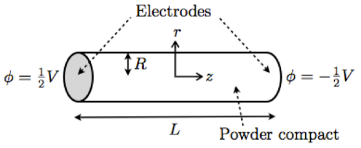
Figure 1: Model set-up considered in this paper. The powder compact is held between two electrodes, at electric potentials $\pm\mbox{$\frac{1}{2}$}V$. Radiative and convective heat loss occurs from the free sides of the cylindrical compact, and from the electrodes.

The electrical conductivity of the ceramic $\sigma(T)$ is a function of temperature $T$, so the electric potential $\phi$ satisfies

$$\nabla\cdot(\sigma(T)\nabla\phi)=0,$$ (1)

with

$$\phi_{r}-R_{z}\phi_{z}=0\quad{\rm at}\quad r=R(z),$$ (2)

$$\phi=\mp\mbox{$\frac{1}{2}$}V\quad{\rm at}\quad z=\pm\mbox{$\frac{1}{2}$}L.$$ (3)

The current is

$$I=-2\pi\int_{0}^{R}\sigma(T)\phi_{z}\,r{\,{\mathrm{d}}{r}},$$ (4)

and is seen from (1) to be independent of $z$. We prescribe either the voltage $V(t)=V_{0}$ or the current $I(t)=I_{0}$; in the latter case the voltage is determined from the integral constraint (4). The experimental procedure usually involves applying a fixed voltage $V_{0}$ initially, but once a maximum current $I_{0}$ is reached, the current is maintained at this value and the voltage is subsequently allowed to vary. Note that contact resistances, between the electrodes and the sample, have been neglected. They are expected to be small and the good agreement between the predictions of this model and the experimental results of [26] would suggest that neglecting them, as has been done by other authors, is reasonable. We should also note that this is the first stage in our investigation and such resistances could be easily included in more sophisticated models. However, their values are not known and to be included accurately these would have to be measured.

The thermal problem is

$$\rho cT_{t}=\nabla\cdot(k\nabla T)+\sigma(T)|\nabla\phi|^{2},$$ (5)

with

$$k\frac{T_{r}-R_{z}T_{z}}{\sqrt{1+R_{z}^{2}}}=-{h_{s}}(T-T_{\infty})-\epsilon S\left[T^{4}-T_{\infty}^{4}\right]\quad{\rm at}\quad r=R(z),$$ (6)

$$\pm T_{z}=-h_{e}(T-T_{\infty})\quad{\rm at}\quad z=\pm\mbox{$\frac{1}{2}$}L\,,\quad\mbox{ and }\quad T=T_{\infty}\,\mbox{ at }\,t=0.$$ (7)

Here $\rho$ is the density of the ceramic powder, $c$ is the specific heat capacity, and $k$ is the thermal conductivity. These are treated as constants. Cooling from the sides of the sample is taken to be through a combination of radiation, with emissivity $\epsilon$, Stefan-Boltzmann constant $S$, and furnace temperature $T_{\infty}$, and conduction/convection, which is parameterized by a heat transfer coefficient $h_{s}$. Cooling from the ends (at the electrodes) is described by a heat transfer coefficient $h_{e}$. The last condition in (7) assumes that the sample is initially at the furnace temperature everywhere.

The electrical conductivity is an increasing function of temperature. We assume the Arrhenius law,

$$\sigma(T)=A{\mathrm{e}}^{-E/R_{g}T},$$ (8)

where $E$ is the activation energy and $R_{g}$ the universal gas constant.

2.2 The dimensionless model

Our axisymmetric models cover some of the bone-shaped samples used in many experiments (see, for example, [7]). However, because of the preliminary nature of the present investigation, here we concentrate on the case of cylindrical symmetry so that there is uniform radius $r=R$, as in the experiments of [15] and [27]. It is intended that situations with $R$ varying with $z$ will be considered in a forthcoming work.

The variables are non-dimensionalised by putting

$$z=L\hat{z},\quad r=R\hat{z},\quad t=t_{0}\hat{t},\quad T=T_{0}+\Delta T\;\!{\theta},\quad$$

$$\phi=V_{0}\hat{\phi},\quad V=V_{0}\hat{V},\quad I=\frac{\sigma_{0}V_{0}\pi R^{2}}{L}\hat{I},\quad\sigma(T)=\sigma_{0}\hat{\sigma}(\theta),\quad$$ (9)

where we choose the thermal-conduction time scale $t_{0}={\rho cR^{2}}/{k}$, the electrical-conductivity scale $\sigma_{0}=A{\mathrm{e}}^{-E/R_{g}T_{0}}$, a sensible choice for $T_{0}$ is the furnace temperature $T_{\infty}$, and we take the temperature perturbation scale $\Delta T=R_{g}T_{0}^{2}/E$ so that the dimensionless conductivity is

$$\hat{\sigma}(\theta)={\mathrm{e}}^{\theta/(1+\nu\theta)},\qquad\nu=\frac{R_{g}T_{0}}{E}.$$ (10)

The parameter $\nu$ is typically small, so we make the approximation $\nu\to 0$, as is standard for treatments of chemical reactions (the Frank-Kamenetskii approximation).

Dropping hats, the resulting model for the electric field is

$$\delta^{2}\left[{\mathrm{e}}^{\theta}\phi_{z}\right]_{z}+\frac{1}{r}\left[r{\mathrm{e}}^{\theta}\phi_{r}\right]_{r}=0,$$ (11)

$$\phi_{r}=0\quad{\rm at}\quad r=1,$$ (12)

$$\phi=\mp\mbox{$\frac{1}{2}$}V\quad{\rm at}\quad z=\pm\mbox{$\frac{1}{2}$},$$ (13)

and for the temperature,

$$\theta_{t}=\delta^{2}\theta_{zz}+\frac{1}{r}\left[r\theta_{r}\right]_{r}+\lambda{\mathrm{e}}^{\theta}\left(\phi_{z}^{2}+\frac{1}{\delta^{2}}\phi_{r}^{2}\right),$$ (14)

$$\theta_{r}=-{\beta}\theta\quad{\rm at}\quad r=1,$$ (15)

$$\theta_{z}=\mp{\alpha}\theta\quad{\rm at}\quad z=\pm\mbox{$\frac{1}{2}$}\,,\,\mbox{ and }\quad\theta=0\,\mbox{ at }\,t=0.$$ (16)

Note that as well as neglecting terms in $\nu$ from the exponential in (14), terms in $\nu$ have also been dropped from (15).

The dimensionless current and its maximum value are given by

$$I=-2\int_{0}^{R}{\mathrm{e}}^{\theta}\phi_{z}\,r{\,{\mathrm{d}}{r}}\leq\mathcal{I},\qquad\mathcal{I}=\frac{I_{0}L}{\sigma_{0}V_{0}\pi R^{2}}.$$ (17)

The other dimensionless parameters in the model are:

$$\delta=\frac{R}{L},\qquad\lambda=\frac{\sigma_{0}V_{0}^{2}R^{2}}{k\Delta TL^{2}},\qquad{\beta=\frac{h_{s}R+4\epsilon ST_{0}^{3}R}{k},\qquad\alpha=\frac{h_{e}L}{k}}$$ (18)

representing the aspect ratio, the strength of the ohmic heating, the combined strength of conductive and radiative cooling from the sides, and strength of cooling from the ends. Typical values are shown in Table 1, although there is significant uncertainty in the values for experimental samples, particularly in the appropriate parameters for the Arrhenius law. Note that the dominant contribution to cooling from the sides comes from the radiation term.

$\rho$	Sample density	$6050\ \textrm{kg}\ \textrm{m}^{-3}$
$c$	Specific heat	$600\ \textrm{J}\ \textrm{kg}^{-1}\ \textrm{K}^{-1}$
$k$	Thermal conductivity	$2.7\ \textrm{J}\ \textrm{m}^{-1}\ \textrm{s}^{-1}\ \textrm{K}^{-1}$
$\epsilon$	Emissivity	$0.7$
$S$	Stefan-Boltzmann constant	$5.67\times 10^{-8}\ \textrm{W}\ \textrm{m}^{-2}\ \textrm{K}^{-4}$
$h_{s}$	Side heat transfer coefficient	$10\ \textrm{J}\ \textrm{m}^{-2}\ \textrm{s}^{-1}\ \textrm{K}^{-1}$
$h_{e}$	Electrode heat transfer coefficient	$10\ \textrm{J}\ \textrm{m}^{-2}\ \textrm{s}^{-1}\ \textrm{K}^{-1}$
$A$	Arrhenius rate factor	$9.3\times 10^{5}\ \textrm{S}\ \textrm{m}^{-1}$
$E$	Activation energy	$171\ \textrm{kJ}\ \textrm{mol}^{-1}$
$R_{g}$	Gas constant	$8.31\ \textrm{J}\ \textrm{K}^{-1}\ \textrm{mol}^{-1}$

$L$	Sample length	$10\ \textrm{mm}$
$R$	Sample radius	$1.5\ \textrm{mm}$
$T_{\infty}$	Furnace temperature	$1110\,{\,\mathrm{K}}$
$V_{0}$	Initial voltage	$300\ \textrm{V}$
$I_{0}$	Current limit	$0.5\ \textrm{A}$
$\sigma_{0}$	Conductivity at $T_{\infty}$	$8.30\times 10^{-3}\ \textrm{S}\ \textrm{m}^{-1}$
$t_{0}$	Time scale	$3.025\ \textrm{s}$

$\delta$	$0.15$
$\lambda$	$0.104$
$\beta$	$0.126$
$\alpha$	$0.037$
$\mathcal{I}$	$284$
$\nu$	$0.054$

Table 1: Typical parameter values and scales used for non-dimensionalisation, along with the corresponding dimensionless parameters. Experimental values for 3YSZ (3 mol % yttria stabilised zirconia) are from [26], along with their Arrhenius fit for the conductivity. An appropriate value for the electrode heat transfer coefficient may vary enormously; we take the same as for the sides for illustration.

General mathematical results on existence and blow-up of solutions of the coupled equations (1) and (5), or equivalently (11) and (14), subject to more limited boundary conditions, can be found in, for example, [2]. However, our approach here will be to simplify the model, given the sizes of parameters in Table 1, so that we can be more specific about the qualitative behaviour of temperature and electric current and obtain relatively simple criteria for the occurrence of flash. In particular, we consider two limiting cases in which the problem is effectively reduced to one spatial dimension. First, we take the case of thermally insulating electrodes, $\alpha=0$, in which case $\theta=\theta(r,t)$. Secondly, we take the case of weakly cooled sides, $\beta=0$, in which case $\theta=\theta(z,t)$. Next we consider the case (as for the estimated values in Table 1) when the heating $\lambda$, as well as the cooling rates $\alpha$ and $\beta$, are all small. Finally, we look at the high-aspect-ratio limit, $\delta$ small.

3 Reduced Models

3.1 Thermally insulating electrodes

If the electrodes remove heat slowly, or heat transfer between them and the sample is poor, we can regard them as providing thermal insulation to the ends. This corresponds to taking $\alpha=0$, and indeed the small value of $\alpha$ in Table 1 suggests this as a possible simplification. In that case there is nothing to induce any $z$-dependence of the temperature so we have $\theta=\theta(r,t)$, $\phi=\phi(z,t)$, and the aspect ratio $\delta$ is removed from the problem. Integrating (11) we obtain

$$\phi=-Vz,\qquad I=2V\int_{0}^{1}{\mathrm{e}}^{\theta}\,r{\,{\mathrm{d}}{r}}.$$ (1)

The heating term becomes $V^{2}{\mathrm{e}}^{\theta}$, and, remembering that either $V=1$ or $I=\mathcal{I}$, we have

$$V={\rm min}\left(1\,,{\mathcal{I}}\Big{/}\left(2\int_{0}^{1}{\mathrm{e}}^{\theta}r{\,{\mathrm{d}}{r}}\right)\right).$$ (2)

Thus the problem for the temperature is

$$\theta_{t}=\frac{1}{r}\left[r\theta_{r}\right]_{r}+\lambda{\mathrm{e}}^{\theta},$$ (3)

$$\mbox{with }\,\theta_{r}=-\beta\theta\quad{\rm at}\quad r=1\,,\,\mbox{ and }\quad\theta=0\,\mbox{ at }\,t=0,$$ (4)

while $2\int_{0}^{1}{\mathrm{e}}^{\theta}r{\,{\mathrm{d}}{r}}\leq\mathcal{I}$. If and when the current limit is reached, the equation switches to

$$\theta_{t}=\frac{1}{r}\left[r\theta_{r}\right]_{r}+\frac{\lambda\mathcal{I}^{2}{\mathrm{e}}^{\theta}}{4(\int_{0}^{1}{\mathrm{e}}^{\theta}r{\,{\mathrm{d}}{r}})^{2}}\,,$$ (5)

with the same boundary conditions. Apart from the switch between voltage and current control, these are standard models; to start with, a semi-linear reaction diffusion problem, and later, a similar problem but with a non-local reaction term. Many results are available concerning the existence of steady states and blow-up solutions.

In particular, for the fixed voltage problem (3)-(4), there is a critical value $\lambda_{c}$ of $\lambda$ above which there is no steady solution, [1, 19]. The critical value can be found from the exact solution,

$$\theta(r)=-2\ln(c-b+br^{2})\,,$$ (6)

where constants $b$ and $c$ are related by

$${\lambda=8b(c-b)\,\,\mbox{ and }\,b=\mbox{$\frac{1}{2}$}\beta c(-\ln c).}$$ (7)

Combining these conditions requires

$$\lambda=4\beta c^{2}(-\ln c)(1+\mbox{$\frac{1}{2}$}\beta\ln c)\,,$$ (8)

which has a solution for $c$ only if $\lambda<\lambda_{c}(\beta)$ (see also [13, 18]). This curve is shown in Figure 2. In particular, $\lambda_{c}\to 2$ for $\beta\to\infty$, while $\lambda_{c}\sim 2\beta/{\mathrm{e}}$ for $\beta\to 0$.

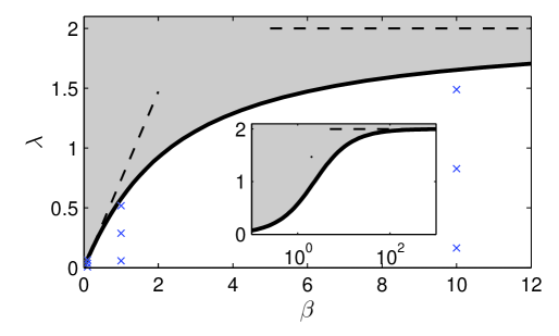
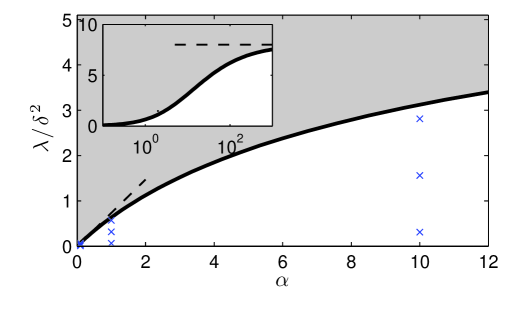
Figure 2: (a) Critical value $\lambda_{c}(\beta)$ for existence of a steady-state solution to (3)-(4). Dashed lines show the asymptotic behaviour and the inset shows the same on a logarithmic scale. (b) Critical value $\Lambda_{c}(\alpha)$ for existence of a steady-state solution to (11)-(12).

For values of $\lambda$ greater than $\lambda_{c}$, the solution to (3)-(4) blows up at a finite time, [20], and with this particular initial data it does so at the centre $r=0$, [12], and in a manner that leads to $\int{\mathrm{e}}^{\theta}r{\,{\mathrm{d}}{r}}$ becoming unbounded, [3, 16, 17]. This means, from (1), that the current $I$ would become large, and that the switch to the current-controlled problem would necessarily occur before blow-up occurs. With large values of the limiting current, so that under current control the sample is rapidly sintered, the incipient blow-up behaviour can be identified as both a necessary and a sufficient condition for the flash process in the constant-voltage phase of a typical experiment, since the rapid heating guarantees that the high temperatures are reached and is also needed to generate them. (For more related results on problems such as (3)-(4), see [5]). In § 4 we discuss the interpretation of these conclusions, and how they may be related to experimental parameters.

The problem under current control, (4)-(5), is not so well studied, since it has a non-local term, but it is known to have a solution which is global in time, and tends to a unique steady state, [4] (see also [21, 22, 11]). The steady state is given by the same formula as above, (6), but now with

$$\lambda\mathcal{I}^{2}=\frac{4\beta(-\ln c)}{c^{2}(1+\mbox{$\frac{1}{2}$}\beta\ln c)}\quad\mbox{ for }\,{\mathrm{e}}^{-2/\beta}<c<1\,.$$ (9)

Contrary to the voltage-controlled problem, this has a solution for $c$ regardless of the value of $\lambda$, so the steady state always exists.

Figure 3 shows the steady-state dimensionless temperature profiles for the voltage-controlled problem (3)-(4) for $\lambda<\lambda_{c}$, and Figure 4 shows steady states for the current-controlled problem (4)-(5). An important prediction of Figure 4 from a practical point of view is that although current control gives stability there can still be considerable temperature gradients within the specimen. Figure 5 shows results from numerical solutions to the full problem (3)-(5), showing the centre ($r=0$) and surface ($r=1$) temperatures for three different values of $\beta$. The final case is subcritical, so the switch to current control is never achieved and the temperature stays close to the furnace temperature.

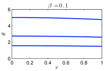
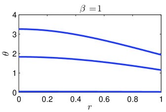
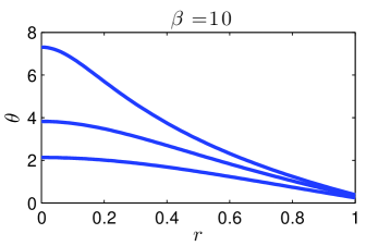
Figure 3: Steady states of the voltage-controlled problem (3)-(4) for $\beta=0.1,1,10$, and $\lambda=(0.1,0.5,0.9)\times\lambda_{c}(\beta)$, as shown by crosses on Figure 2.

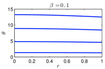
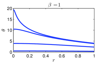
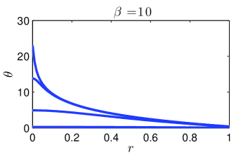
Figure 4: Steady states of the current-controlled problem (4)-(5) for $\beta=0.1,1,10$, and $\lambda\mathcal{I}^{2}=1,10^{2},10^{4},10^{6}$ (larger $\theta$ for larger $\lambda\mathcal{I}^{2}$).

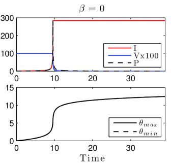
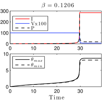
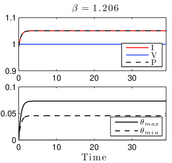
Figure 5: Numerical solutions to (2)-(4) using three different values of $\beta$, and with $\lambda=0.104$, $\mathcal{I}=284$. Top panels show evolution of current, voltage, and power $P=IV$. Lower panels show the maximum and minimum temperature (at the centre line and outer radius, respectively). Incipient blow-up, limited by the current limit, is clearly seen in the first two cases.

3.2 Thermally insulating sides

Based on the parameter values in Table 1, which indicate that cooling from the sides is rather weak, another limiting case to consider is to set $\beta=0$. For more generality, however, we now conversely allow for the possibility of cooling from the electrodes, with $\alpha>0$. If the electrodes are very good conductors of heat they may effectively be held at the furnace temperature $T_{\infty}$ in which case $\alpha\to\infty$.

In this case there is nothing to induce any $r$ dependence of the temperature, we have $\theta=\theta(z,t)$, and the electric problem (11) has solution

$$\phi_{z}=I{\mathrm{e}}^{-\theta},\qquad V=I\int_{-\mbox{$\frac{1}{2}$}}^{\mbox{$\frac{1}{2}$}}{\mathrm{e}}^{-\theta}\,{\rm d}z.$$ (10)

The initial voltage-controlled temperature problem ($V=1$) is therefore

$$\theta_{t}=\delta^{2}\theta_{zz}+\lambda\frac{{\mathrm{e}}^{-\theta}}{\left(\int_{-1/2}^{1/2}{\mathrm{e}}^{-\theta}{\,{\mathrm{d}}{z}}\right)^{2}}\,,$$ (11)

$$\theta_{z}=\mp\alpha\theta\quad{\rm at}\quad z=\pm\mbox{$\frac{1}{2}$},\qquad\theta=0\quad{\rm at}\quad t=0.$$ (12)

Unlike in the previous section, it is now this voltage-controlled regime which has a non-local term. Moreover, in this case, the non-local reaction term can lead to blow-up of $\theta$ for all $z$ and hence to blow-up of current ([21, 22]; see below also), and thus there is a switch to current control. If the end cooling is sufficiently strong, however, the problem may tend towards a steady state with no blow-up occurring.

If the switch to current-control is achieved, the equation becomes simply

$$\theta_{t}=\delta^{2}\theta_{zz}+\lambda\mathcal{I}^{2}{\mathrm{e}}^{-\theta}\,,\qquad$$ (13)

which is a standard reaction-diffusion problem. With the reaction term decreasing in $\theta$, this problem has a unique equilibrium, to which all solutions approach for large time (see [25]).

For flash to happen in this model therefore requires blow-up to occur for (11), and we determine the conditions under which this will happen by again seeking a steady-state solution. If such a solution exists, then blow-up does not occur. The steady state satisfies

$$\delta^{2}\theta_{zz}+\lambda\frac{{\mathrm{e}}^{-\theta}}{\left(\int_{-1/2}^{1/2}{\mathrm{e}}^{-\theta}{\,{\mathrm{d}}{z}}\right)^{2}}=0\,,\qquad\theta_{z}=\mp\alpha\theta\quad{\rm at}\quad z=\pm\mbox{$\frac{1}{2}$}\,,$$ (14)

and the solution is

$$\theta(z)=2\ln\left(\frac{\cos az}{\cos\mbox{$\frac{1}{2}$}a}\right)+b$$ (15)

where the constants $a$ and $b$ are related by

$$\frac{\lambda}{\delta^{2}}=8{\mathrm{e}}^{-b}\sin^{2}\mbox{$\frac{1}{2}$}a\,,\qquad b=\frac{2a}{\alpha}\tan\mbox{$\frac{1}{2}$}a.$$ (16)

There is a solution for $a$ only if $\lambda\leq\delta^{2}\Lambda_{c}(\alpha)$, where $\Lambda_{c}(\alpha)$ is shown in Figure 2. Solutions of (11)-(12) for $\lambda$ less than this critical value are displayed in Figure 6. It is straightforward to determine that $\Lambda_{c}\to 8$ for $\alpha\to\infty$, and $\Lambda_{c}\sim 2\alpha/{\mathrm{e}}$ for $\alpha\to 0$.

Steady states for (13) have the same form as in (15), but with

$$\frac{\lambda\mathcal{I}^{2}}{\delta^{2}}=\frac{2a^{2}}{\cos^{2}\mbox{$\frac{1}{2}$}a}\,e^{b},\qquad b=\frac{2a}{\alpha}\tan\mbox{$\frac{1}{2}$}a$$ (17)

and some sample cases can be seen in Figure 7.

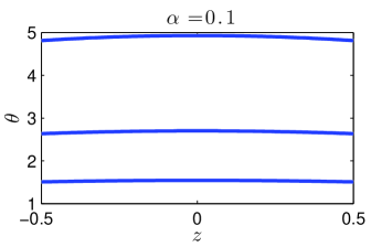
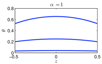
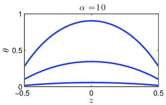
Figure 6: Steady states of the voltage-controlled problem (11)-(12) for $\alpha=0.1,1,10$, and $\lambda=(0.1,0.5,0.9)\times\lambda_{c}(\beta)$, as shown by crosses on Figure 2.

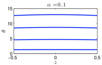
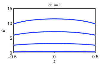
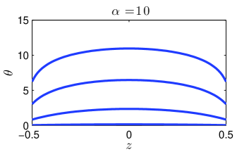
Figure 7: Steady states of the current-controlled problem (12)-(13) for $\alpha=0.1,1,10$, and $\lambda\mathcal{I}^{2}=1,10^{2},10^{4},10^{6}$ (larger $\theta$ for larger $\lambda\mathcal{I}^{2}$).

3.3 Analysis for small $\alpha$, $\beta$ and $\lambda$

If $\alpha=\beta=0$ in (11)-(16), the temperature is independent of space, and $\phi=-Vz$, with $V=\min\left(1,\mathcal{I}/e^{\theta}\right)$. Concentrating solely on the voltage-controlled regime, it is clear that the problem exhibits blow-up as $t\to 1/\lambda$ according to

$$\theta=-\log(1-\lambda t).$$ (18)

Such blow-up can only be prevented if the cooling terms are in fact non-negligible, and $\lambda$ is not too large. Thus, we consider the case when $\alpha$, $\beta$ and $\lambda$ are all comparably small. In this case the temperature is still roughly uniform over the cross-section, and it is appropriate to integrate over the whole domain, giving

$$\frac{{\rm d}\theta}{{\rm d}t}=f(\theta)-g(\theta),$$ (19)

where the ‘bulk’ heating and cooling functions are

$$f(\theta)=\lambda\min\left({\mathrm{e}}^{\theta},\mathcal{I}^{2}{\mathrm{e}}^{-\theta}\right),\qquad g(\theta)=2\left(\beta+\delta^{2}\alpha\right)\theta,$$ (20)

the cooling terms coming from the side and the ends, respectively.

The heat balance (19) provides a simple way to understand the process. Graphs of $f(\theta)$ and $g(\theta)$ are given in Figure 8 and indicate how the temperature might evolve towards a steady state for which $f(\theta)=g(\theta)$. Flash sintering requires that a sufficiently high temperature is exceeded before we reach this steady state. In practice, we expect that this temperature is high enough that the current-limited regime must always be reached, implying that there must be no steady state on the voltage-controlled portion of the heating curve. The absence of such a steady state is the condition that blow-up would occur, were it not for the current limit.

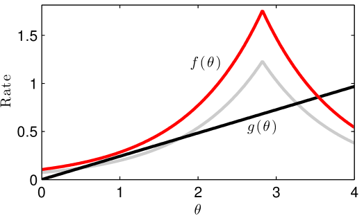
Figure 8: Heating and cooling functions from (20). The cooling curve $g(\theta)$ is shown in black, and the heating curve $f(\theta)$ is shown in red, for the parameter values in Table 1. The steady-state temperature is given by the intersection of the two curves. In grey is the heating curve for a smaller (subcritical) value of $\lambda$.

More precisely, the blow-up condition is that the increasing portion of the red curve in the Figure 8 lies above the black curve. Otherwise, a steady state will be reached at too low a temperature. This critical condition can be expressed as

$$\lambda>(2/{\mathrm{e}})(\beta+\delta^{2}\alpha)\,,$$ (21)

which is found from the condition that the $f(\theta)$ and $g(\theta)$ curves meet tangentially. This is consistent with the limiting behaviour of $\lambda_{c}(\beta)$ and $\Lambda_{c}(\alpha)$ for small $\beta$ and $\alpha$ found in the previous two sections.

If the current limit $\mathcal{I}$ is too low it is clear that even the steady state that occurs in the current-limited regime (which always exists, since $f(\theta)\to 0$ for $\theta\to\infty$) will be at too low a temperature for sintering. Thus $\mathcal{I}$ must not be made too small, but it is otherwise unimportant with regard to the occurrence of flash.

3.4 High aspect ratio

We now consider the case when $\delta$ is small, which provides a link between the previous three subsections.

If $\delta$ is small, but $\alpha$, $\beta$ and $\lambda$ are order one, then the cooling effect of the electrodes is confined to boundary layers at the edges. In that case the bulk of the sample has temperature independent of $z$ and the analysis of Subsection 3.1 applies. On the other hand, if $\alpha$, $\beta$ and $\lambda$ are also small, the problem is essentially the same as in Subsection 3.3, and that analysis applies.

If, $\delta$, $\beta$ and $\lambda$ are small, but $\alpha$ is order one (or even infinite, for the case of highly conductive electrodes held at the furnace temperature), another reduction applies. In that case the temperature is roughly uniform across the radius, and an integral over the cross-section produces the dimensionless model, in the case of voltage control,

$$\theta_{\tilde{t}}=\theta_{zz}+\Lambda\left(\int_{-1/2}^{1/2}{\mathrm{e}}^{-\theta}{\,{\mathrm{d}}{z}}\right)^{-2}{\mathrm{e}}^{-\theta}-B\theta\,,\qquad\theta_{z}=\mp\alpha\theta\quad{\rm at}\quad z=\pm\mbox{$\frac{1}{2}$},$$ (22)

where

$$\tilde{t}=\delta^{2}t,\quad{\Lambda=\lambda/\delta^{2}\quad\mbox{ and }}\quad B=2\beta/\delta^{2}\,.$$ (23)

After flash (the occurrence of which is discussed below), the current-controlled model becomes, more simply,

$$\theta_{\tilde{t}}=\theta_{zz}+\Lambda\mathcal{I}^{2}{\mathrm{e}}^{-\theta}-B\theta\,,\qquad\theta_{z}=\mp\alpha\theta\quad{\rm at}\quad z=\pm\mbox{$\frac{1}{2}$},$$ (24)

which is a standard reaction-diffusion problem. As for (13), there is a unique equilibrium for this current-controlled problem, which all solutions approach for large time (see [25]).

To determine whether flash happens, we want to know if blow-up will occur for the voltage-controlled problem (22). Once again this will occur if $\Lambda$ is sufficiently large, and the critical condition in this case becomes

$$\Lambda>{\tilde{\Lambda}}_{c}(\alpha,B)\,.$$ (25)

To determine this critical value, we seek a steady-state solution, for which

$$\theta_{zz}+\Lambda\left(\int_{-1/2}^{1/2}{\mathrm{e}}^{-\theta}{\,{\mathrm{d}}{z}}\right)^{-2}{\mathrm{e}}^{-\theta}-B\theta=0\,,\qquad\theta_{z}=\mp\alpha\theta\quad{\rm at}\quad z=\pm\mbox{$\frac{1}{2}$}\,.$$ (26)

If such a solution exists, then blow-up does not occur. Given the form of (26), it is difficult to calculate such a solution analytically and thus determine the critical value ${\tilde{\Lambda}}_{c}(\alpha,B)$ leading to flash. However, a lower bound can be obtained by neglecting either the first or third term in (26).

In the case that $B$ is large (as is the case for the data in Table 1), the cooling effect of the electrodes is again confined to diffusive boundary layers at the edges. Over most of the sample the temperature is then approximately the same as in Subsection 3.3, and that earlier analysis shows that $\tilde{\Lambda}_{c}\approx B/e$. If $B$ is small, on the other hand, then (26) reduces to the same problem as in (11)-(12), and the analysis of Subsection 3.2 applies, showing $\tilde{\Lambda}_{c}\approx\Lambda_{c}(\alpha)$.

4 Conclusions

We have described a mathematical model for the process of flash sintering based on Joule heating, and investigated its behaviour in a simple cylindrically symmetric geometry. Numerical and approximate analytical solutions are consistent with experimental results for flash sintering [26].

For certain limiting cases of the parameters, the problem may be reduced to one spatial dimension and, depending on whether voltage or current is controlled, the equations can take the form of a local or non-local reaction diffusion problem. We have made use of existing results concerning the solutions of such problems to infer that flash sintering manifests itself as incipient blow-up behaviour, and we can identify the controlling processes that determine whether such behaviour occurs. In all cases this is a competition between the rate of heating (controlled experimentally by voltage), and the rate of cooling (predominantly by radiation). An automatic switch between voltage and current control in the experiments prevents blow-up from actually occurring, and the model suggests that once this switch has occurred, the temperature distribution within the sample evolves towards a stable steady state. It is clear that the current limit must be set sufficiently high so that the temperatures needed for rapid sintering to occur are achieved.

The most appropriate of our reduced models to the experimental results appears to be the case of thermally insulating electrodes, for which we derived the condition $\lambda>\lambda_{c}(\beta)$ for a flash to occur, where $\lambda$ is the dimensionless heating parameter, $\beta$ the dimensionless cooling parameter, and the function $\lambda_{c}(\beta)$ is shown in Figure 2. Converted back into dimensional terms, this condition is given as

$$\left(\frac{R^{2}AE}{kR_{g}T_{\infty}^{2}}\right)\left(\frac{V}{L}\right)^{2}{\mathrm{e}}^{-E/(R_{g}T_{\infty})}>\lambda_{c}\left(\frac{R{h_{s}}+4R\epsilon ST_{\infty}^{3}}{k}\right).$$ (1)

This is expressed as a regime diagram in terms of furnace temperature and voltage as shown in Figure 9, where the theroretical predictions are compared with the experimental results of [26]. We note that Figure 9 is similar to Figure 5 of [26] but that there is some systematic overestimate of the critical potential gradient at lower temperatures. Observe that condition (1) also demonstrates the dependence on the geometry and other parameters. For instance, increasing the radius of the sample would make flash more likely.

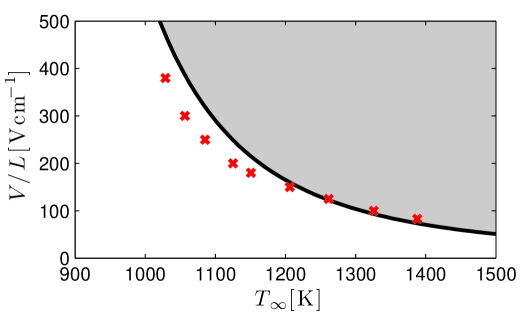
Figure 9: Critical condition (1) for blow-up of (3)-(4) in terms of dimensional furnace temperature $T_{\infty}$ and electric field $V/L$, all other parameters being held at constant values from Table 1. Flash occurs in the grey region. The red crosses indicate experimental values from [26].

The model also suggests that before any flash occurs, the temperature is fairly uniform across the sample, and in that case Figure 8 describes the essential behaviour quite succinctly. The form of the red heating curve is determined by the form of $\sigma(T)$, which was approximated, from an Arrhenius function, by an exponential. Literature estimates for the conductivity and its dependence on temperature vary considerably, however, so this simple analysis of blow-up may prove useful to investigate other functional forms for $\sigma(T)$.

If incipient ‘blow-up’ starts and the current limit is large enough not to kick in for some time, the conclusion that the temperature is almost uniform across the sample will no longer hold true. This is because the temperature is largest in the centre of the sample, and leads to faster heating there. This issue could be investigated further by studying the asymptotics of near blow-up for small $\beta$, and large $\mathcal{I}$, although the local form of such single-point blow-up has already been looked at, for example, in [3, 16, 17]: it might be expected, from consideration of a similarity solution near blow-up at $r=0$, that the solution of an equation such as (3) would have a profile at the blow-up time of $\theta\sim-2\ln r$ + constant for $r$ small; however, no suitable similarity solution exists and the usual profile at blow-up time is somewhat spikier than might be expected, $\theta\sim-2\ln r+\ln(-\ln r)$ + constant. From the experimental point of view it is of interest to know what the maximum temperature is, and what the temperature differential within the material is. In this context, it is worth noting that greater temperature variations across the sample are produced for large $\lambda$, $\mathcal{I}$ and $\beta$ (see the eventual steady states in Figures 4 and 7).

Another issue that should be studied further in the future is the effect of non-uniform cross-section. By forcing a non-uniform electric current through the sample, this may induce a more complex pattern of heating and enable understanding of experimental problems associated with partial or incomplete sintering.

References

- [1] H. Amann. Fixed point equations and nonlinear eigenvalue problems in ordered Banach spaces. SIAM Rev., 18 (1976), 620–709.
- [2] S.N. Antontsev, M. Chipot. Analysis of blowup for the thermistor problem. Siberian. Math. Jl., 38 (1997), 827–841.
- [3] J. Bebernes, S. Bricher. Final time blowup profiles for semilinear parabolic equations via center manifold theory. SIAM Jl. Math. Anal., 23 (1992), No. 4, 852–869.
- [4] J. Bebernes, A.A. Lacey. Global existence and finite-time blow-up for a class of nonlocal parabolic problems. Adv. Diff. Eqns., 2 (1997), No. 6, 927–53.
- [5] J. Bebernes, D.Eberly. Mathematical problems from combustion theory. Springer, New York, 1989.
- [6] G. Cimatti. The stationary thermistor problem with a current limiting device. Proc. Roy. Soc. Edin., 116A (1990), 79–84.
- [7] M. Cologna, B. Rashkova, R. Raj. Flash sintering of nanograin zirconia in s at C. J. Am. Ceram. Soc., 93 (2010), No. 11, 3556–3559.
- [8] A.C. Fowler, I. Frigaard, S.D. Howison. Temperature surges in current-limiting circuit devices. SIAM Jl. Appl. Math., 52 (1992), 998–1011.
- [9] J.S.C. Francis, M. Cologna, R. Raj. Particle size effects in flash sintering. J. Eur. Ceram. Soc., 32 (2012), 3129–3136.
- [10] J.S.C. Francis, R. Raj. Influence of the field and the current limit on flash sintering at isothermal furnace temperatures. J. Eur. Ceram. Soc., 96 (2013), No. 9, 2754–2758.
- [11] P. Freitas. A nonlocal Sturm-Liouville eigenvalue problem. Proc. Roy. Soc. Ed., 124A (1994), No. 1, 169–188.
- [12] A. Friedman, B. McLeod. Blowup of positive solutions of semilinear heat equations. Indiana Univ. Jl. Maths., 34 (1985), 425–477.
- [13] I.M. Gelfand. Some problems in the theory of quasilinear equations. Amer. Math. Soc. Trans., 29 (1963), 295–381.
- [14] S. Grasso, Y. Sakka, N. Redntorff, C. Hu, G. Maizza, H. Borodianska, O. Vasylkiv. Modeling of the temperature distribution of flash sintered zirconia. J. Ceram. Soc. Japan, 119 (2011), No. 2, 144–146.
- [15] S. Grasso, T. Saunders, H. Porwal, O. Cedillos-Barraza, D. D. Jayaseelan, W. E. Lee, M. J. Reece. Flash Spark Plasma Sintering (FSPS) of Pure ZrB2. J. Am. Ceram. Soc., 97 (2014), No. 8, 2405–2408.
- [16] M.A. Herrero, J.J.L. Velázquez. Blow-up profiles in one-dimensional. semilinear parabolic problems. Coms. PDEs., 17 (1992), No. 3, 205–219.
- [17] M.A. Herrero, J.J.L. Velázquez. Plane structures in thermal runaway. Israel Jl. Maths., 81 (1993), No. 3, 321–341.
- [18] D.D. Joseph, T.S. Lundgren. Quasilinear Dirichlet problems driven by positive sources. Arch. Rat. Mech. Anal., 49 (1973), 241–269.
- [19] H.B. Keller, D.S. Cohen. Some positone problems suggested by nonlinear heat generation. Jl. Math. Mech., 16 (1967), 1361–1376.
- [20] A.A. Lacey. Mathematical analysis of thermal runaway for spatially inhomogeneous reactions. SIAM Jl. Appl. Maths., 43 (1983), 1350–1366.
- [21] A.A. Lacey. Thermal runaway in a non-local problem modelling ohmic heating. I: Model derivation and some special cases. Eu. Jl. Appl. Maths., 6 (1995), 127–144.
- [22] A.A. Lacey. Thermal runaway in a non-local problem modelling ohmic heating. II: General proof of blow-up and asymptotics of runaway. Eu. Jl. Appl. Maths., 6 (1995), 201–224.
- [23] K.S. Naik, V.M. Sglavo, R. Raj. Flash sintering as a nucleation phenomenon and a model thereof. J. Eur. Ceram. Soc., 34 (2014), 4063–4067.
- [24] R. Raj. Joule heating during flash-sintering. J. Eur. Ceram. Soc., 32 (2012), 2293–2301.
- [25] D. Sattinger. Monotone methods in nonlinear elliptic and parabolic boundary value problems. Indiana Univ. Math. Jl., 21 (1972), 979–1000.
- [26] R.I. Todd, E. Zapata-Solvas, R.S. Bonilla, T. Sneddon, P.R. Wilshaw. Electrical characteristics of flash sintering: thermal runaway of Joule heating. To appear in J. Eur. Ceram. Soc. (2015).
- [27] E. Zapata-Solvas, S. Bonilla, P.R. Wilshaw, R.I. Todd. Preliminary investigation of flash sintering of SiC. J. Eur. Ceram. Soc., 33 (2013), 2811–2816.