$1/f$ noise from the nonlinear transformations of the variables

Abstract

The origin of the low-frequency noise with power spectrum $1/f^{\beta}$ (also known as $1/f$ fluctuations or flicker noise) remains a challenge. Recently, the nonlinear stochastic differential equations for modeling $1/f^{\beta}$ noise have been proposed and analyzed. Here we use the self-similarity properties of this model with respect to the nonlinear transformations of the variable of these equations and show that $1/f^{\beta}$ noise of the observable may yield from the power-law transformations of well-known standard processes, like the Brownian motion, Bessel and similar stochastic processes. Analytical and numerical investigations of such techniques for modeling processes with $1/f^{\beta}$ fluctuations is presented.

I Introduction

Different theories and models have been proposed for explanation of the ubiquitous $1/f^{\beta}$ noise phenomena, observable for about eighty years in different systems from physics to financial markets (see, e.g., Refs. Weissman1988 ; Gisiger2001 ; Li2012 ; Balandin2013 ; Paladino2014 ; Kaulakys2009 ; Ruseckas2014 ; Rodriguez2014 and references herein). Recently, the stochastic model of $1/f^{\beta}$ noise, based on the nonlinear stochastic differential equations

$$dx=\left(\eta-\frac{\lambda}{2}\right)x^{2\eta-1}dt+x^{\eta}dW_{t}\,,$$ (1)

where $x$ is the signal with $1/f^{\beta}$ spectrum, $\eta\neq 1$ is the nonlinearity exponent, $\lambda$ is the exponent of the steady-state distribution $P_{\mathrm{ss}}\sim x^{-\lambda}$, and $W_{t}$ is a Wiener process (Brownian motion), has been proposed and analyzed.Kaulakys2009 ; Ruseckas2014 The relation of the exponent $\beta$ in the spectrum to the parameters of Eq. (1) is given by

$$\beta=1+\frac{\lambda-3}{2(\eta-1)}\,.$$ (2)

Eq. (1) may be derived from the point process model Kaulakys2009 , from scaling properties of the signal Ruseckas2014 or from the agent-based herding model Ruseckas2011 .

Here we employ the self-similarity property of Eq. (1) with respect the power-law transformations of the variable. We show that processes with $1/f^{\beta}$ spectrum may yield from the nonlinear transformations of the variable of the widespread processes, e.g., from the Brownian motion, Bessel or similar familiar processes.

II Transformations

From the scaling of the power spectral density (PSD) $S(f)\sim f^{-\beta}$,

$$S(af)\sim a^{-\beta}S(f)\,,$$ (3)

according to the Wiener-Khintchine theorem yields the scaling of the autocorrelation function

$$C(at)\sim a^{\beta-1}C(t)$$ (4)

in some time interval $1/f_{\mathrm{max}}\ll t\ll 1/f_{\mathrm{min}}$. Recently Ruseckas2014 it was shown that from the scaling (4) it follows the nonlinear stochastic differential equation (SDE) (1). Due to this scaling the nonlinear SDE

$$dx=\left(\eta_{x}-\frac{\lambda_{x}}{2}\right)x^{2\eta_{x}-1}dt+x^{\eta_{x}}dW_{t}\,,$$ (5)

generating signal $x$ with PSD

$$S(f)\sim\frac{1}{f^{\beta_{x}}}\,,\qquad\beta_{x}=1+\frac{\lambda_{x}-3}{2(\eta_{x}-1)}$$ (6)

after the nonlinear transformation

$$x=\frac{1}{y^{\delta}}\,,$$ (7)

with $\delta$ being the transformation exponent, yields SDE for the variable $y$ of the same form,

$$dy=\left(\eta_{y}-\frac{\lambda_{y}}{2}\right)x^{2\eta_{y}-1}dt+y^{\eta_{y}}dW_{t}$$ (8)

with

$$\eta_{y}=1-\delta(\eta_{x}-1)\,,\qquad\lambda_{y}=1-\delta(\lambda_{x}-1)\,.$$ (9)

Eq. (8) generates signal $y$ with the PSD

$$S(f)\sim\frac{1}{f^{\beta_{y}}}\,,\qquad\beta_{y}=1+\frac{\lambda_{y}-3}{2(\eta_{y}-1)}=\beta_{x}+\frac{1+\delta}{\delta(\eta_{x}-1)}\,.$$ (10)

Therefore, $1/f^{\beta_{x}}$ noise of the observable $x$ may yield from the nonlinear dependence (7) of this observable on another variable $y$ resulted from simple or more common equation (8), where

$$\beta_{x}=\beta_{y}+\frac{1+\delta}{\eta_{y}-1}\,.$$ (11)

III Examples

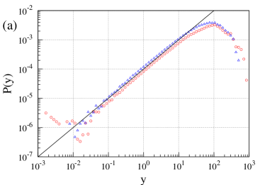
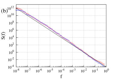
Figure 1: Steady-state distribution, (a), and approximately $1/f^{2}$ PSD, (b), of the variable $y$ generated by the simple equation (12), red circles, as well as of $y=1/x$ generated by Eq. (13), blue triangles, with the appropriate restrictionsRuseckas2014 of the diffusion intervals.

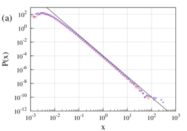
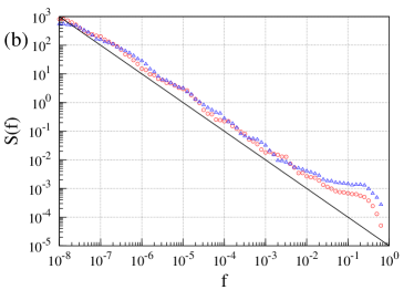
Figure 2: Steady-state distribution, (a), and $1/f$ PSD, (b), of the observable $x=1/y$, where the variable $y$ is generated by Eq. (12), red circles, as well as of $x$ generated by Eq. (13), blue triangles.

Figure 3: Examples of the signals of 1D Brownian motion of the variable $y$, (a), of the inverse 1D Brownian motion of the observable $x=1/y$ yielding in $1/\sqrt{f}$ noise, (b), and of $x=1/\sqrt{y}$ observable resulting in pure $1/f$ noise, (c).

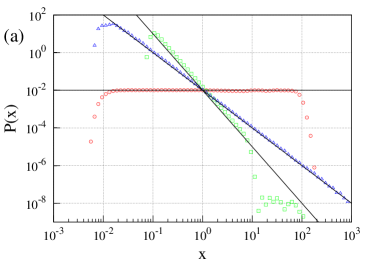
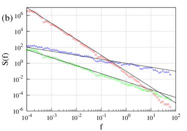
Figure 4: Steady-state distribution, (a), and PSD, (b), of 1D Brownian motion of the variable $y$, yielding $1/f^{2}$ noise, red circles, the inverse 1D Brownian motion of $x=1/y$ yielding in $1/\sqrt{f}$ noise, blue triangles, and of the observable $x=1/\sqrt{y}$ resulting in pure $1/f$ noise, green squares.

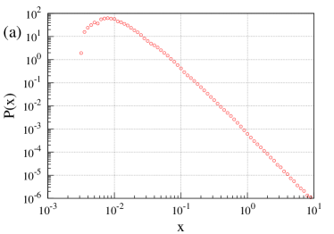
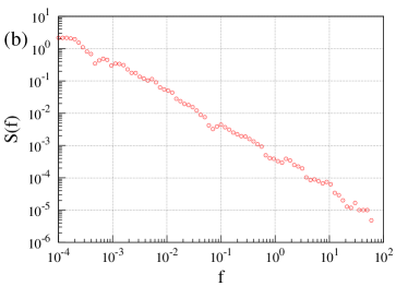
Figure 5: Steady-state distribution, (a), and PSD, (b), of the observable $x$ as inverse of the distance from the beginning, $x=1/r$, of the Brownian motion in 2D.

The simplest relation between the variable $y$ and the observable $x$ is the inverse transformation $x=1/y$. From the interrelations (10) and (11) between the parameters $\beta_{x}$ and $\beta_{y}$ we obtain that simple equation without the drift term

$$dy=\frac{1}{\sqrt{y}}dW_{t}$$ (12)

results in $1/f$ noise of the observable $x=1/y$, instead of very nonlinear equation Kaulakys2004

$$dx=x^{4}dt+x^{5/2}dW_{t}$$ (13)

for the observable $x$. It should be noted, that Eq. (12) coincides with equation for the interevent time

$$d\tau=\frac{1}{\sqrt{\tau}}dW_{t}\,,$$ (14)

obtained form the Brownian motion

$$d\tau_{k}=dW_{k}$$ (15)

of the interevent time $\tau_{k}$ in the events space or $k$-space.Kaulakys2004

Figures 1 and 2 demonstrate the appearance of $1/f$ noise of the observable $x$, as a result of the inverse transformation $x=1/y$ of the variable $y$ generated by the simple equation without the drift term (12) with approximate $1/f^{2}$ PSD of the variable $y$.

Note, that special cases of Eq. (8) are: (i) an equation with the additive noise, $\eta_{y}=0$, and nonlinear drift, i.e., the Bessel process of order $N=1-\lambda_{y}$, (ii) the order $N=2(1-\lambda_{y})$ squared Bessel process when $\eta_{y}=1/2$ and $\lambda_{y}=1-N/2$, (iii) the special exponential restrictions of the variable $y$ in Eq. (8) yield Constant Elasticity of Variance (CEV) process or (iv) Cox-Ingersoll-Ross (CIR) process when $\eta=1/2$ Ruseckas2011 ; Jeanblanc2009 .

Here we will demonstrate the possibility to obtain $1/f^{\beta}$ noise from the Bessel process and from the Brownian motion. Transformation (7) with $\delta=1/(\eta_{x}-1)$, i.e., $y=x^{1-\eta_{x}}$, yields the special form of Eq. (8), i.e., the Bessel equation

$$dy=\frac{N-1}{2}\frac{dt}{y}+dW_{t}$$ (16)

corresponding to $N$-dimensional Wiener process, or Bessel process with index $\nu=N/2-1$. Here

$$N=\frac{\lambda_{x}-1}{\eta_{x}-1}=1-\lambda_{y}\,.$$ (17)

On the other hand

$$\lambda_{x}=1+\frac{N}{\delta}\,,\qquad\beta_{x}=1+\frac{N}{2}-\delta\,.$$ (18)

Thus, the Bessel process or $N$-dimensional Brownian motion can cause $1/f^{\beta}$ fluctuations of the observable $x$ as a function (7) of this process. So, the pure $1/f$ noise yields when $N=2\delta$, e.g., from 1D Brownian motion of $y$ for the observable $x=1/\sqrt{y}$ and 2D Brownian motion of $y$ for the observable $x=1/y$.

Figure 3 demonstrates examples of the signals of 1D Brownian motion of the variable $y$, the inverse 1D Brownian motion of $x=1/y$ yielding in $1/\sqrt{f}$ noise and observable $x=1/\sqrt{y}$ resulting in pure $1/f$ noise. In figure 4 the distribution density and PSD of the corresponding observables are presented.

In figure 5 the pure $1/f$ noise of the observable $x$ as inverse of the distance from the beginning, $x=1/r$, of the Brownian motion in 2D,

$$r=\sqrt{B_{1}^{2}\left(t\right)+B_{2}^{2}\left(t\right)}\,,$$ (19)

i.e., of the Bessel process with the index $\nu=0$ is shown. Here $B_{1}\left(t\right)$ and $B_{2}\left(t\right)$ are independent Brownian motions. We see the pure $1/f$ noise.

IV Conclusions

Thus, the proper function of the widespread process, e.g., the inverse transformation of the order 2 Bessel process and the inverse square root of the Brownian motion yield the pure 1/f noise, observable, e.g., in condense matter. Possible relevancies of these transformations to $1/f$ noise in condensed matter: (i) $1/f$ fluctuations of the voltage, $U=I/G$, at constant current $I$ as a result of Brownian fluctuations of the conductivity $G$, (ii) $1/f$ fluctuations of resistivity, $\rho=1/\sigma$, as Brownian fluctuations of the conductivity $\sigma$.

References

- (1) M. B. Weissman, Rev. Mod. Phys. 60 (1988) 537.
- (2) T. Gisiger, Biol. Rev. 76 (2001) 161.
- (3) M. Li and W. Zhao, Math. Probl. Engin. 2012 (2012) 673648.
- (4) A. A. Balandin,Nature Nanotechnol. 8 (2013) 549.
- (5) E. Paladino, Y. M. Galperin, G. Falci, and B. L. Altshuler, Rev. Mod. Phys. 86 (2014) 361.
- (6) B. Kaulakys and M. Alaburda, J. Stat. Mech. 2009 (2009) P02051.
- (7) J. Ruseckas and B. Kaulakys, J. Stat. Mech. 2014 (2014) P06005.
- (8) M. A. Rodriguez, Phys. Rev. E 90 (2014) 042122.
- (9) J. Ruseckas, B. Kaulakys and V. Gontis, EPL 96 (2011) 60007.
- (10) B. Kaulakys and J. Ruseckas, Phys. Rev. E 70 (2004) 020101.
- (11) M. Jeanblanc, M. Yor and M. Chesney Mathematical Methods for Financial Markets (Springer, London, 2009).