Fully relativistic multiple scattering calculations for general potentials

Abstract

The formal basis for fully relativistic Korringa-Kohn-Rostoker (KKR) or multiple scattering calculations for the electronic Green function in case of a general potential is discussed. Simple criteria are given to identify situations that require to distinguish between right and left hand side solutions to the Dirac equation when setting up the electronic Green function. In addition various technical aspects of an implementation of the relativistic KKR for general local and non-local potentials will be discussed.

I Introduction

Recently there is strong interest in the impact of spin-orbit coupling on the electronic structure of solids and surfaces as this gives rise to many interesting and technically important phenomena. In this context one may mention the well known magneto-crystalline anisotropy but also the interesting galvano-magnetic and spin transport phenomena.RMS09 ; LGK+11 ; TGFM12 ; ZCK+14 Other examples for the central role of spin-orbit coupling can be found in the field of spectroscopy as the magneto-optical effects and the various magneto-dichroic phenomena in X-ray spectroscopy.Ebe96b ; HE02a ; VRW+04 Finally one may mention the Rashba splittingAPM+08 ; BMK+14 of surface states of transition metals as well as occurrence of the topological surface states in topological insulators.HK10 ; QZ11

Computational schemes used to describe these phenomena or materials, respectively, have to account at the same time for spin-orbit coupling, spin polarization or magnetic ordering as well as the structural properties of the investigated system in a coherent and reliable way. Among the various available schemes the Korringa-Kohn-Rostoker (KKR) or multiple scattering method is especially attractive as it gives direct access to the Green function (GF). Making use of the Dyson equation allows for example by means of the corresponding embedding technique to deal with rather complex systems.EKM11 Another important field of application for the KKR-GF method is the investigation of disordered systems usually done in combination with the Coherent Potential Approximation (CPA) Sov67 alloy theory.

The spin-polarized relativistic (SPR) version of the KKR method set up on the basis of the four-component Dirac formalism that allows to account for all relativistic effects and spin magnetism within the framework of L(S)DA (local (spin) density approximation) on equal footing was worked out by various authors.FRA83 ; SSG84 Extensions to this approach were made to deal with orbital polarization EB96 as well as the presence of a vector potential coupling to the total current of the electrons.EBG97 ; BMB+12 Corresponding implementations and applications of the KKR method were done in general making use of the ASA (Atomic Sphere Approximation) that implies spherical symmetry for the potential functions and rotational symmetry for the corresponding vector fields coupling to the spin and current of the electrons. Finally, the so-called full potential (FP) version of the SPR-KKR method that removes the mentioned geometrical restrictions was discussed and implemented by various authors.Tam92 ; LGG93 ; WZB+92 ; HZE+98

Compared to the non-relativistic version of the KKR method its fully relativistic formulation leads to a number of technical complications. The need to distinguish between right (RHS) and left hand side (LHS) solutions to the Dirac equation was discussed in particular by Tamura Tam92 for the case of a general local potential. Here we extend this work discussing among others the impact of a non-local site-diagonal potential and several practical aspects of corresponding KKR calculations.

II Relativistic Hamiltonian and Green function for general potentials

Starting point of our considerations is an effective one-electron Hamiltonian $\hat{\cal H}(z)$ that can be split into an energy-independent, Hermitian part $\hat{\cal H}^{1}$ and an energy-dependent, non-Hermitian part:

$$\hat{\cal H}(z) = \hat{\cal H}^{1}+\hat{\Sigma}(z)$$ (1)

$$= \hat{\cal H}^{0}+\hat{\cal V}+\hat{\Sigma}(z)$$ (2)

with the Hermitian adjoined operator

$$\hat{\cal H}^{\dagger}(z) = \hat{\cal H}^{0\dagger}+\hat{\cal V}^{\dagger}+\hat{\Sigma}^{\dagger}(z)$$ (3)

$$= \hat{\cal H}^{0}+\hat{\cal V}+\hat{\Sigma}(z^{*})\;.$$ (4)

Here $\hat{\cal H}^{0}$ stands for the Hamiltonian of the free-electron system, $\hat{\cal V}$ for an energy independent Hermitian potential and the non-Hermitian self-energy $\Sigma(z)$ may depend on the energy $z$. Using a fully relativistic formulation based on the four-component Dirac formalism the real space representation of $\hat{\cal H}^{1}$ takes the form:Ros61

$$\hat{\cal H}^{1}(\mathbf{r}) = -ic\mbox{\boldmath${\alpha}$}\cdot\mbox{\boldmath${\nabla}$}+\frac{1}{2}\,c^{2}(\beta-1)+V(\mathbf{r})$$ (6)

$$= i\gamma_{s}\sigma_{r}c\left(\frac{\partial}{\partial r}+\frac{1}{r}-\frac{\beta}{r}\,K\right)$$

$$\qquad\qquad\quad+\frac{1}{2}\,c^{2}(\beta-1)+V(\mathbf{r})$$

with $\alpha_{i}$ (see below) and $\beta$ the standard $4\times 4$ Dirac matrices, $K$ the spin-orbit operator, $\sigma_{r}=\mbox{\boldmath${\sigma}$}\cdot\mathbf{r}/r$ the projection of the Pauli matrices and

$$\gamma_{s}=\left(\begin{array}[]{cc}0&-I_{2}\\ -I_{2}&0\end{array}\right)\;.$$ (7)

In Eq. (6) atomic Rydberg units ($\hbar=1$, $e^{2}=2$, $m=1/2$) have been used and the rest mass energy $c^{2}/2$ has been subtracted from the energy $z$. The potential $V(\mathbf{r})$ is assumed to be local and in the most general case it will be a $4\times 4$ matrix function according to:

$$V(\mathbf{r}) = \bar{V}(\mathbf{r})+\beta\,\mbox{\boldmath${\sigma}$}\cdot\mathbf{B}(\mathbf{r})+e\mbox{\boldmath${\alpha}$}\cdot\mathbf{A}(\mathbf{r})$$ (8)

$$= \bar{V}(\mathbf{r})+\left(\begin{array}[]{cc}\mbox{\boldmath${\sigma}$}\cdot\mathbf{B}(\mathbf{r})&0\\ 0&-\mbox{\boldmath${\sigma}$}\cdot\mathbf{B}(\mathbf{r})\end{array}\right)$$ (14)

$$\quad\quad+e\left(\begin{array}[]{cc}0&\mbox{\boldmath${\sigma}$}\cdot\mathbf{A}(\mathbf{r})\\ \mbox{\boldmath${\sigma}$}\cdot\mathbf{A}(\mathbf{r})&0\end{array}\right)$$

$$= \left(\begin{array}[]{cc}V^{+}(\mathbf{r})&U(\mathbf{r})\\ U(\mathbf{r})&V^{-}(\mathbf{r})\end{array}\right)\;.$$ (17)

Here $\bar{V}(\mathbf{r})$ and $\beta\,\mbox{\boldmath${\sigma}$}\cdot\mathbf{B}(\mathbf{r})$ stand for the spin-independent and spin-dependent parts of the potential, respectively, while the term $e\mbox{\boldmath${\alpha}$}\cdot\mathbf{A}(\mathbf{r})$ represents the coupling of a vector potential $\mathbf{A}(\mathbf{r})$ to the electronic current density, with ${\alpha}$ the electronic velocity operator.Ros61 Obviously, the auxiliary potential functions $V^{\pm}(\mathbf{r})$ and $U(\mathbf{r})$ are $2\times 2$ matrix functions in spin space.Tam92

For the real space representation of the self energy $\Sigma(z)$ one again has in general a $4\times 4$ matrix function $\Sigma(\mathbf{r},\mathbf{r}\,^{\prime},z)$ that may be written in an analogous way:

$$\Sigma(\mathbf{r},\mathbf{r}\,^{\prime},z) = \Sigma^{V}\,(\mathbf{r},\mathbf{r}\,^{\prime},z)+\beta\,\mbox{\boldmath${\sigma}$}\,\mathbf{\Sigma}^{B}\,(\mathbf{r},\mathbf{r}\,^{\prime},z)$$ (18)

$$= \left(\begin{array}[]{cc}\Sigma^{+}(\mathbf{r},\mathbf{r}\,^{\prime},z)&0\\ 0&\Sigma^{-}(\mathbf{r},\mathbf{r}\,^{\prime},z)\end{array}\right)\;,$$ (21)

where we restrict to a spin-dependent self-energy. A current-dependent one coupling like $\mbox{\boldmath${\alpha}$}\cdot\mathbf{\Sigma}^{A}$ could be introduced as well and treated in analogy to the term $\mbox{\boldmath${\sigma}$}\cdot\mathbf{A}(\mathbf{r})$ in the local potential. From Eqs.  (3) and (4) one has for $\Sigma(\mathbf{r},\mathbf{r}\,^{\prime},z)$ the property:

$$\Sigma^{\dagger}(\mathbf{r},\mathbf{r}\,^{\prime},z) = \Sigma(\mathbf{r}\,^{\prime},\mathbf{r},z^{*})\;.$$ (22)

In practice it seems to be sufficient for most applications to consider a self-energy $\Sigma(\mathbf{r},\mathbf{r}\,^{\prime},z)$ that can be represented by an expansion into a product of suitable basis functions:

$$\Sigma(\mathbf{r},\mathbf{r}\,^{\prime},z) = \sum_{\Lambda\Lambda^{\prime}}\phi_{\Lambda}(\mathbf{r})\,\Sigma_{\Lambda\Lambda^{\prime}}(z)\,\phi_{\Lambda^{\prime}}^{\dagger}(\mathbf{r}\,^{\prime})\;.$$ (23)

In line with the relativistic representation the basis functions $\phi_{\Lambda}(\mathbf{r})$ are constructed here as four-component functions with the index $\Lambda$ specifying their spin-angular character Ros61 (see below).

Explicit forms for the local potential $V(\mathbf{r})$ as given by Eq. (8) can be derived within the framework of relativistic density functional theory (DFT).ED11 ; Esc96 Dealing with magnetic solids the relativistic version of the local spin density approximation (LSDA) to DFT is usually adopted.MV79 ; RR79 ; ED11 This scheme is derived by applying a Gordon decomposition of the electronic current density into its spin and orbital contribution and retaining only the corresponding spin-dependent part of the Hamiltonian.RC73 ; MV79 The term in Eq. (8) involving the vector potential $\mathbf{A}(\mathbf{r})$ may be derived within current density functional theory (CDFT) VR87 ; Die91 that in particular accounts for the electronic orbital degrees of freedom. Alternatively or in addition, it may represent the Breit interaction ED11 that plays a prominent role for the magneto-crystalline anisotropy.Jan88a

While the non-local self-energy $\Sigma(\mathbf{r},\mathbf{r}\,^{\prime},z)$ in Eq. (18) may stand for example for the energy-independent Hartree-Fock potential, it will in general represent extensions to the standard relativistic LSDA scheme. Within spectroscopic investigations, life-time effects are usually represented by an optical potential corresponding to a local but complex and energy-dependent potential.TF86 Alternatively or in addition, $\Sigma(\mathbf{r},\mathbf{r}\,^{\prime},z)$ may represent correlation effects that are not accounted for by standard LSDA. Within the rather simple L(S)DA+U scheme AZA91 , the corresponding non-local self-energy is real and energy-independent. On the other hand, the combination of the more sophisticated dynamical mean field theory (DMFT) GKKR96 ; Hel07 with the LSDA implies a complex and energy-dependent non-local self-energy. For both schemes one restricts usually to local correlations corresponding to a site-diagonal self-energy (see below). This restriction is dropped e.g. for cluster variants of the DMFT GKKR96 and does not apply to the standard formulation of the GW method.AG98

The Green function operator $\hat{G}(z)$ associated with the general Hamiltonian $\hat{\cal H}(z)$ in Eqs. (1) to (4) is defined to be simultaneously the right and left inverse of $\big{(}z-\hat{\cal H}(z)\big{)}$:

$$\left(z-\hat{\cal H}(z)\right)\,\hat{G}(z) = 1$$ (24)

$$\hat{G}(z)\,\left(z-\hat{\cal H}(z)\right) = 1$$ (25)

implying the relation:

$$\hat{G}^{\dagger}(z) = \hat{G}(z^{*})\;.$$ (26)

In their real space representation Eqs.  (24) through (26) read:

$$\left(z\,-\hat{\cal H}^{1}(\mathbf{r})\right)\,G(\mathbf{r},\mathbf{r}\,^{\prime},z)\hskip 42.67912pt$$

$$-\int d^{3}r\,^{\prime\prime}\,\Sigma(\mathbf{r},\mathbf{r}\,^{\prime\prime},z)\,G(\mathbf{r}\,^{\prime\prime},\mathbf{r}\,^{\prime},z) = {{1}}_{4}\,\delta(\mathbf{r}\,,\mathbf{r}\,^{\prime})$$ (27)

$$\delta(\mathbf{r},\mathbf{r}\,^{\prime})\,{{1}}_{4} = G(\mathbf{r},\mathbf{r}\,^{\prime},z)\left(z-\hat{\cal H}^{1}(\mathbf{r}\,^{\prime})\right)$$ (28)

$$-\int d^{3}r\,^{\prime\prime}\,G(\mathbf{r},\mathbf{r}\,^{\prime\prime},z)\,\Sigma(\mathbf{r}\,^{\prime\prime},\mathbf{r}\,^{\prime},z)$$

$$G^{\dagger}(\mathbf{r},\mathbf{r}\,^{\prime},z) = G(\mathbf{r}\,^{\prime},\mathbf{r},z^{*})\;.$$ (29)

The differential operator contained in $\hat{\cal H}^{1}(\mathbf{r}\,^{\prime})$ in Eq. (28) has to be interpreted to act to the left. The more familiar right hand side form can be obtained by taking the Hermitian adjoint of this equation and making use of Eqs. (22) and (29):

$$\left(z^{*}-\hat{\cal H}^{1}(\mathbf{r}\,^{\prime})\right)\,G(\mathbf{r}\,^{\prime},\mathbf{r},z^{*})\hskip 42.67912pt$$

$$-\int d^{3}r\,^{\prime\prime}\,\Sigma(\mathbf{r}\,^{\prime},\mathbf{r}\,^{\prime\prime},z^{*})\,G(\mathbf{r}\,^{\prime\prime},\mathbf{r},z^{*}) = \delta(\mathbf{r}\,,\mathbf{r}\,^{\prime})\,{{1}}_{4}\;.$$ (30)

Obviously, replacing $z^{*}$ by $z$ the original right hand side equation (II) is recovered.

As shown for the non-relativistic case by various authors,HFL87 ; Lay63 an expression for the Green function defined by the Eqs. (II) and (28) can be given also for the relativistic case in terms of a spectral representation:

$$G(\mathbf{r},\mathbf{r}\,^{\prime},z)=\sum_{n}\,\frac{\phi_{n}(\mathbf{r},z)\,\psi_{n}^{\dagger}(\mathbf{r}\,^{\prime},z)}{z-E_{n}(z)}\;.$$ (31)

Here the so-called right- and left-hand side solutions, $\phi_{n}(\mathbf{r},z)$ and $\psi_{n}(\mathbf{r},z)$, respectively, are four component functions (bi-spinors) and defined as solutions to the following eigenvalue equations

$$\left(E_{n}(z)-\hat{\cal H}^{1}(\mathbf{r})\right)\,\phi_{n}(\mathbf{r},z)\hskip 59.75095pt$$

$$-\int d^{3}r\,\Sigma(\mathbf{r},\mathbf{r}\,^{\prime},z)\,\phi_{n}(\mathbf{r}\,^{\prime},z) = 0$$ (32)

$$\left(E_{n}(z)^{*}-\hat{\cal H}^{1}(\mathbf{r})\right)\,\psi_{n}(\mathbf{r},z)\hskip 59.75095pt$$

$$-\int d^{3}r\,^{\prime}\,\Sigma(\mathbf{r},\mathbf{r}\,^{\prime},z^{*})\,\psi_{n}(\mathbf{r}\,^{\prime},z) = 0$$ (33)

that have in general complex eigenvalues $E_{n}(z)$. On the basis of Eqs. (II) and (II), it is straightforward to show that Eq. (31) is indeed a solution to Eqs. (II) and (28). In this context it is interesting to note that the homogeneous term ${{1}}_{4}\,\delta(\mathbf{r}\,,\mathbf{r}\,^{\prime})$ in these equations is ensured to be covered by the closure relation

$$\sum_{n}\phi_{n}(\mathbf{r},z)\,\psi_{n}^{\dagger}(\mathbf{r}\,^{\prime},z) = {1}_{4}\,\delta(\mathbf{r},\mathbf{r}\,^{\prime})\;.$$ (34)

In case of a non-vanishing energy dependent self-energy $\Sigma(\mathbf{r},\mathbf{r}\,^{\prime},z)$, the set of eigenvalue equations (II) and (II) has obviously to be solved for each value of energy $z$. For that reason the spectral representation given in Eq. (31) may not be very helpful in practice. Nevertheless, it clearly shows that even in case of a non-vanishing $\Sigma(\mathbf{r},\mathbf{r}\,^{\prime},z)$, a real space representation of the Green function can in principle be given.

III Multiple scattering or KKR representation of the Green function

The multiple scattering or KKR-GF formalism aims to supply the Green function $G(\mathbf{r},\mathbf{r}\,^{\prime},z)$ for a given energy $z$ without making use of the spectral representation given in Eq. (31). Dealing with an extended system as a cluster of atoms or a solid the problem to find the Green function is subdivided by dealing in a first step with the scattering from a single potential well associated with an atom site and treating multiple scattering in a subsequent step. According to this, the discussion below is restricted here to a self-energy $\Sigma(\mathbf{r},\mathbf{r}\,^{\prime},z)$ that is site-diagonal, i.e. $\Sigma(\mathbf{r},\mathbf{r}\,^{\prime},z)=0$ for $\mathbf{r}$ or $\mathbf{r}\,^{\prime}$ outside the regime of the considered potential well. More complex situations can nevertheless be treated by making use of the Dyson equation.NKH+12 Furthermore, only on-the-energy-shell scattering will be considered, i.e. inelastic processes will explicitly excluded.

Guided by the eigenvalue equations (II) and (II) connected with the spectral representation Eq. (31) the RHS and LHS solutions to the so-called single site Dirac equation will be considered first. From these the single-site t-matrix and Green function will be derived. Finally, the multiple scattering will be considered leading to the Green function of the total system.

III.1 RHS and LHS solutions to the Dirac equation

The RHS solutions $|\psi(z)\rangle$ to the Dirac equation for a given energy $z$ are defined by

$$\big{(}z-\hat{\cal H}(z)\big{)}\,|\psi(z)\rangle=0\;.$$ (35)

With the real space representation of the Hamilton operator $\hat{\cal H}(z)$ given by Eqs.  (6) and (18) this corresponds for the wave function $\psi_{\nu}(\mathbf{r},z)$ labeled by the index ${\nu}$ to the equation

$$\hat{\cal H}^{1}(\mathbf{r})\,\psi_{\nu}(\mathbf{r},z)-\int d^{3}r\,^{\prime}\,\Sigma(\mathbf{r},\mathbf{r}\,^{\prime},z)\,\psi_{\nu}(\mathbf{r}\,^{\prime},z) =$$

$$\Bigg{[}z-i\gamma_{s}\sigma_{r}c\left(\frac{\partial}{\partial r}+\frac{1}{r}-\frac{\beta}{r}\,K\right)\qquad\qquad$$

$$-V(\mathbf{r})-(\beta-1)\,\frac{c^{2}}{2}\Bigg{]}\psi_{\nu}(\mathbf{r},z)$$

$$-\int d^{3}r\,^{\prime}\,\Sigma(\mathbf{r},\mathbf{r}\,^{\prime},z)\,\psi_{\nu}(\mathbf{r}\,^{\prime},z) = 0\;,$$ (36)

where the general potential $V(\mathbf{r})$ and self-energy $\Sigma(\mathbf{r},\mathbf{r}\,^{\prime},z)$ are defined as in Eqs. (8) and (18). As multiple scattering is treated in a most suitable way by working with an angular momentum representation, we make for $\psi_{\nu}(\mathbf{r},z)$ the standard ansatzFRA83 ; SSG84

$$\psi_{\nu}(\mathbf{r},z) = \sum_{\Lambda}\,\psi_{\Lambda\nu}(\mathbf{r},z)$$ (37)

$$= \sum_{\Lambda}\,\left(\begin{array}[]{c}g_{\Lambda\nu}(r,z)\chi_{\Lambda}(\hat{r})\\ i\,f_{\Lambda\nu}(r,z)\chi_{-\Lambda}(\hat{r})\end{array}\right)$$ (40)

with the radial functions $g_{\Lambda\nu}(r,z)$ and $f_{\Lambda\nu}(r,z)$ connected with the large and small, respectively, components of the wave function. The spin-angular function $\chi_{\Lambda}(\hat{r})$ is an eigen function of the spin-orbit operator $K$

$$K\,\chi_{\Lambda}(\hat{r})=-\kappa\,\chi_{\Lambda}(\hat{r})$$ (41)

with the property

$$\sigma_{r}\,\chi_{\Lambda}(\hat{r})=-\chi_{-\Lambda}(\hat{r})\;.$$ (42)

Here we used the short-hand notation $\Lambda=(\kappa,\mu)$ and $-\Lambda=(-\kappa,\mu)$ to give the spin-orbit and magnetic quantum numbers $\kappa$ and $\mu$, respectively.Ros61 The index $\nu$ labeling the linearly independent solutions $\psi_{\nu}(\mathbf{r},z)$ will be dropped in this section. Later on, it will be replaced by a spin-angular index ($\Lambda^{\prime}$) that reflects the asymptotic behavior of the solution $\psi_{\Lambda^{\prime}}(\mathbf{r},z)$.

Inserting the ansatz Eq. (37) into the Dirac Eq. (III.1) one is led after some straightforward manipulations to the following set of radial Dirac equations for the RHS solutions:

$$\left(\begin{array}[]{cc}z&c\,\left(\frac{\partial}{\partial\,r}+\frac{-\kappa+1}{r}\right)\\ c\,\left(\frac{\partial}{\partial\,r}+\frac{\kappa+1}{r}\right)&-(z+c^{2})\end{array}\right)\,\left(\begin{array}[]{r}g_{\Lambda}(r,z)\\ f_{\Lambda}(r,z)\end{array}\right)-\sum_{\Lambda^{\prime}}\left(\begin{array}[]{cc}V_{\Lambda\,\Lambda^{\prime}}^{+}(r)&-i\,U_{\Lambda\,-\Lambda^{\prime}}(r)\\ i\,U_{-\Lambda\,\Lambda^{\prime}}(r)&-V_{-\Lambda\,-\Lambda^{\prime}}^{-}(r)\end{array}\right)\,\left(\begin{array}[]{c}g_{\Lambda^{\prime}}(r,z)\\ f_{\Lambda^{\prime}}(r,z)\end{array}\right)$$ (51)

$$-\sum_{\Lambda^{\prime}}\int r^{\prime 2}\,dr^{\prime}\,\left(\begin{array}[]{c}\Sigma_{\Lambda\,\Lambda^{\prime}}^{+}(r,r\,^{\prime},z)\,\,\,\,\,\,\,g_{\Lambda^{\prime}}(r^{\prime},z)\\ -\Sigma_{-\Lambda\,-\Lambda^{\prime}}^{-}(r,r\,^{\prime},z)\,\,\,f_{\Lambda^{\prime}}(r^{\prime},z)\end{array}\right) = 0\;.$$ (54)

Here we used the matrix element functions connected with the potential

$$V_{\Lambda\,\Lambda^{\prime}}^{\pm}(r) = \int d\hat{r}\,\,\chi_{\Lambda}^{\dagger}(\hat{r})\,V^{\pm}(\mathbf{r})\,\chi_{\Lambda^{\prime}}(\hat{r})$$

$$U_{\Lambda\,\Lambda^{\prime}}(r) = \int d\hat{r}\,\chi_{\Lambda}^{\dagger}(\hat{r})\,\,U(\mathbf{r})\,\chi_{\Lambda^{\prime}}(\hat{r})$$

and the self-energy

$$\Sigma_{\Lambda\,\Lambda^{\prime}}^{\pm}(r,r^{\prime},z)=\int d\hat{r}\,\int d\hat{r}^{\prime}\,\chi_{\Lambda}^{\dagger}(\hat{r})\,\,\Sigma^{\pm}(\mathbf{r},\mathbf{r}\,^{\prime},z)\,\chi_{\Lambda^{\prime}}(\hat{r}\,^{\prime})\;.$$

The LHS solution $\langle\psi^{\times}(z)|$ corresponding to the RHS solution $|\psi(z)\rangle$ is defined by the adjoined Dirac equation

$$\langle\psi^{\times}(z)|\big{(}z-\hat{\cal H}(z)\big{)}=0$$ (55)

with its real space representation given by

$$\langle\psi^{\times}(z)|\mathbf{r}\,^{\prime}\rangle\,\big{(}z-\hat{\cal H}^{1}(\mathbf{r}\,^{\prime})\big{)}\hskip 56.9055pt$$

$$-\int d^{3}r\,^{\prime\prime}\,\,\langle\psi^{\times}(z)|\mathbf{r}\,^{\prime\prime}\rangle\,\Sigma(\mathbf{r}\,^{\prime\prime},\mathbf{r}\,^{\prime},z) = 0\;.$$ (56)

To proceed, we find it more convenient to switch to the Hermitian adjoined of this equation:

$$\big{(}\hat{\cal H}^{1}(\mathbf{r})-z^{*}\big{)}\,\langle\psi^{\times}(z)|\mathbf{r}\rangle^{\dagger}\hskip 56.9055pt$$

$$+\int d^{3}r\,^{\prime}\,\,\Sigma^{\dagger}(\mathbf{r},\mathbf{r}\,^{\prime},z^{*})\,\langle\psi^{\times}(z)|\mathbf{r}\,^{\prime}\rangle^{\dagger} = 0\;,$$ (57)

where use of the relations $\hat{\cal H}^{1}(\mathbf{r})=\hat{\cal H}^{1\dagger}(\mathbf{r})$ and $\Sigma^{\dagger}(\mathbf{r},\mathbf{r}\,^{\prime},z)=\Sigma(\mathbf{r}\,^{\prime},\mathbf{r},z^{*})$ has been made.

Making for $\langle\psi^{\times}(z)|\mathbf{r}\rangle$ the ansatzTF89 ; Tam92

$$\langle\psi^{\times}(z)|\mathbf{r}\,\rangle=\sum_{\Lambda}(g_{\Lambda}^{\times}(r,z)\,\chi_{\Lambda}^{\dagger}(\hat{r}),\,-if_{\Lambda}^{\times}(r,z)\,\chi_{-\Lambda}^{\dagger}(\hat{r}))$$ (58)

one has for its adjoined wave function

$$\langle\psi^{\times}(z)|\mathbf{r}\rangle^{\dagger}=\sum_{\Lambda}\left(\begin{array}[]{r}g_{\Lambda}^{\times*}(r,z)\,\chi_{\Lambda}(\hat{r})\\ if_{\Lambda}^{\times*}(r,z)\,\chi_{-\Lambda}(\hat{r}))\end{array}\right)\;.$$ (61)

Inserting this expression into Eq. (III.1) leads to a set of radial equations that corresponds one-to-one to Eq. (54) apart from the replacements $z\rightarrow z^{*}$, $(g,f)\rightarrow(g^{\times\,*},f^{\times\,*})$, and $\Sigma(\mathbf{r},\mathbf{r}\,^{\prime},z)\rightarrow\Sigma(\mathbf{r},\mathbf{r}\,^{\prime},z^{*})$. Accordingly, Eq. (III.1) can be rearranged as Eq. (54) to lead to the radial Dirac equations for the LHS solutions

$$\left(\begin{array}[]{cc}z&c\,\left(\frac{\partial}{\partial\,r}+\frac{-\kappa+1}{r}\right)\\ c\,\left(\frac{\partial}{\partial\,r}+\frac{\kappa+1}{r}\right)&-(z+c^{2})\end{array}\right)\,\left(\begin{array}[]{r}g_{\Lambda}^{\times}(r,z)\\ f_{\Lambda}^{\times}(r,z)\end{array}\right)-\sum_{\Lambda^{\prime}}\left(\begin{array}[]{cc}V_{\Lambda^{\prime}\,\Lambda}^{+}(r)&i\,U_{-\Lambda^{\prime}\,\Lambda}(r)\\ -i\,U_{\Lambda^{\prime}\,-\Lambda}(r)&-V_{-\Lambda^{\prime}\,-\Lambda}^{-}(r)\end{array}\right)\,\left(\begin{array}[]{c}g_{\Lambda^{\prime}}^{\times}(r,z)\\ f_{\Lambda^{\prime}}^{\times}(r,z)\end{array}\right)$$ (70)

$$-\sum_{\Lambda^{\prime}}\int r^{\prime 2}\,dr^{\prime}\,\left(\begin{array}[]{c}\Sigma_{\Lambda^{\prime}\,\Lambda}^{+}(r\,^{\prime},r,z)\,\,\,\,\,\,\,g_{\Lambda^{\prime}}^{\times}(r^{\prime},z)\\ -\Sigma_{-\Lambda^{\prime}\,-\Lambda}^{-}(r\,^{\prime},r,z)\,\,\,f_{\Lambda^{\prime}}^{\times}(r^{\prime},z)\end{array}\right) = 0\;.$$ (73)

Here use of the relations

$$V_{\Lambda\,\Lambda^{\prime}}^{\pm}(r)^{*} = V_{\Lambda^{\prime}\,\Lambda}^{\pm}(r)$$ (74)

$$U_{\Lambda\,\Lambda^{\prime}}(r)^{*} = U_{\Lambda^{\prime}\,\Lambda}(r)$$ (75)

$$\Sigma_{\Lambda\,\Lambda^{\prime}}^{\pm}(r,r\,^{\prime},z^{*})^{*} = \Sigma_{\Lambda^{\prime}\,\Lambda}^{\pm}(r\,^{\prime},r,z)$$ (76)

has been made that reflect the Hermiticity of the potential (Eq. (8)) as well as the properties of the self-energy (Eq. (18)). Accordingly, the set of radial Dirac equations (54) and (73) for the RHS and LHS, respectively, solutions are identical if the following relations hold:

$$V_{\Lambda\,\Lambda^{\prime}}^{\pm}(r) = V_{\Lambda^{\prime}\,\Lambda}^{\pm}(r)$$ (77)

$$U_{\Lambda\,\Lambda^{\prime}}(r) = -U_{\Lambda^{\prime}\,\Lambda}(r)$$ (78)

$$\Sigma_{\Lambda\,\Lambda^{\prime}}^{\pm}(r,r\,^{\prime},z) = \Sigma_{\Lambda^{\prime}\,\Lambda}^{\pm}(r\,^{\prime},r,z)\;.$$ (79)

Ignoring the self-energy for the moment, the resulting set of radial Dirac equations in Eqs. (54) and (73) are completely equivalent to those obtained by Tamura Tam92 . Accordingly, the requirements given by him for the RHS and LHS equations being the same coincide with Eqs. (77) and (78). A more detailed discussion under what conditions these relations hold will be given in the next section.

Finally, it should be mentioned that in the context of the relativistic L(S)DA+U EPM03 as well as L(S)DA+DMFT MCP+05 Eq. (54) or (73), resp., has been dealt with so far in an approximate way. Because for both schemes the coupling of the self-energy is usually restricted to the d- or f-electrons and because the basis functions for the self-energy (see Eq. (23)) have the same $l$-character, it seems justified to interchange the role of the radial functions to be calculated and of the basis functions. This transfers the radial integro-differential equations into differential equations as they occur in the case of full potential type calculations HZE+98 . As a consequence, the set up of the corresponding Green function simplifies in a dramatic way as can be seen from the discussions in section III.6.

III.2 Relation between the RHS and LHS solutions

As the RHS and LHS solutions derive from the same Hamiltonian, it is obvious that they are not independent from each other. In fact, the vector space spanned by the LHS solutions is dual to that spanned by the RHS solutions. In particular, TamuraTam92 could show that the RHS and LHS solutions are connected via

$$\langle\psi^{\times}(\mathbf{B})|=\left(\hat{K}\,|\psi(-\mathbf{B})\rangle\right)^{\dagger}$$ (80)

by making use of the behavior of the Hamiltonian $\hat{\cal H}(\mathbf{B})$ under time reversal $\hat{K}$. This implies for the radial functions the relationsTam92

$$\left(\begin{array}[]{r}g_{\kappa\mu}^{\times}(r,z,\mathbf{B})\\ f_{\kappa\mu}^{\times}(r,z,\mathbf{B})\end{array}\right)=(-1)^{\mu-1/2}S_{\kappa}\,\left(\begin{array}[]{r}g_{\kappa-\mu}(r,z,-\mathbf{B})\\ f_{\kappa-\mu}(r,z,-\mathbf{B})\end{array}\right)\;,$$ (85)

where $S_{\kappa}$ stands for the sign of the quantum number $\kappa$Ros61 and the vector $\mathbf{B}$ represents also the dependence of the wave functions on the vector potential $\mathbf{A}$ as well as the spin dependent part of the self-energy $\Sigma$ that also reverse sign under time reversal.

Eq. (85) shows that for non-magnetic systems ($\mathbf{B}=0$), having time reversal symmetry, LHS radial functions for $\Lambda=({\kappa,\mu})$ that solve Eq.  (73) can easily be obtained from the RHS radial functions for $\Lambda=({\kappa,-\mu})$ by multiplying with the phase factor $(-1)^{\mu-1/2}S_{\kappa}$. For magnetic systems ($\mathbf{B}\neq 0$), on the other hand, it may happen that the two sets of radial functions have to be calculated individually (see section IV).

In both cases, however, the sets of radial differential equations for the LHS and RHS solutions, Eqs.  (54) and (73), respectively, are identical if the various potential functions $V_{\Lambda\Lambda^{\prime}}^{\pm}(r)$, $U_{\Lambda\Lambda^{\prime}}^{\pm}(r)$, and $\Sigma_{\Lambda\Lambda^{\prime}}^{\pm}(r,r^{\prime},z)$ are symmetric (see Eqs. (77) to (79)). Accordingly both sets of equations will be solved by the same set of linearly independent (unnormalized) radial functions, i.e. these have to be determined only once. To see under which conditions this favorable situation holds, we restrict for the moment to the case $\Sigma_{\Lambda\Lambda^{\prime}}^{\pm}(r,r^{\prime},z)=0$ and expand the real potentials $\bar{V}(\mathbf{r})$, $\mathbf{B}(\mathbf{r})$, and $\mathbf{A}(\mathbf{r})$ in terms of real spherical harmonics ${\cal Y}_{L}(\hat{r})$ according to:

$$\bar{V}(\mathbf{r}) = \sum_{L}\,V_{L}(r)\,{\cal Y}_{L}(\hat{r})$$ (86)

$$\mathbf{B}(\mathbf{r}) = \sum_{L}\,\sum_{\lambda}B_{L}^{\lambda}(r)\,{\cal Y}_{L}(\hat{r})\,\hat{e}_{\lambda}$$ (87)

$$\mathbf{A}(\mathbf{r}) = \sum_{L}\,\sum_{\lambda}A_{L}^{\lambda}(r)\,{\cal Y}_{L}(\hat{r})\,\hat{e}_{\lambda}$$ (88)

one has for their matrix elements:

$$V_{\Lambda\Lambda^{\prime}}^{\pm}(r) = \sum_{L}\Big{(}\bar{V}_{L}(r)\,\langle\chi_{\Lambda}|{\cal Y}_{L}|\chi_{\Lambda^{\prime}}\rangle$$ (89)

$$\qquad\quad\pm\sum_{\lambda}\,B_{L}^{\lambda}(r)\,\langle\chi_{\Lambda}|\sigma_{\lambda}\,{\cal Y}_{L}|\chi_{\Lambda^{\prime}}\rangle\Big{)}$$

$$U_{\Lambda\Lambda^{\prime}}(r) = \sum_{L}\sum_{\lambda}A_{L}^{\lambda}(r)\,\langle\chi_{\Lambda}|\sigma_{\lambda}\,{\cal Y}_{L}|\chi_{\Lambda^{\prime}}\rangle\;,$$ (90)

with real functions $\bar{V}_{L}(r)$, $B_{L}^{\lambda}(r)$ and $A_{L}^{\lambda}(r)$ and $\lambda$ indicating the components of the vector fields with $\hat{e}_{\lambda}$ the corresponding unit vector. For the angular matrix elements occurring in Eqs. (89) and (90) one has the property

$$\langle\chi_{\Lambda}|{\cal Y}_{L}|\chi_{\Lambda^{\prime}}\rangle = \langle\chi_{\Lambda^{\prime}}|{\cal Y}_{L}|\chi_{\Lambda}\rangle^{*}$$

$$\langle\chi_{\Lambda}|\sigma_{\lambda}\,{\cal Y}_{L}|\chi_{\Lambda^{\prime}}\rangle = \langle\chi_{\Lambda^{\prime}}|\sigma_{\lambda}\,{\cal Y}_{L}|\chi_{\Lambda}\rangle^{*}$$

ensuring the Hermiticity of the corresponding potential terms.

For the special cases $m(L)\geq 0$ and $\lambda=x,$ or $z$ one finds in particular that the angular matrix elements are real, implying that they are symmetric w.r.t. the indices $\Lambda$ and $\Lambda^{\prime}$. Having only such terms in the expansions in Eqs.  (89) and (90) also the corresponding potential matrix elements are symmetric, i.e. the requirement specified in Eqs.  (77) to (78) for the LHS and RHS solutions being identical are fulfilled. The conditions for this to happen are discussed in some detail in section IV.5.

Finally, Eq. (79) will in general not hold for a finite self-energy $\Sigma(\mathbf{r},\mathbf{r}\,^{\prime},z)$ and accordingly one has to determine the RHS and LHS solutions on the basis Eqs.  (54) and (73), separately. Assuming for $\Sigma(\mathbf{r},\mathbf{r}\,^{\prime},z)$ an expansion as given by Eq. (23) with the basis functions $\phi_{\Lambda}(\mathbf{r})$ involving real radial functions, the requirement expressed by Eq. (79) reduces to the simpler relation:

$$\Sigma^{\pm}_{\Lambda\Lambda^{\prime}}(z)=\Sigma^{\pm}_{\Lambda^{\prime}\Lambda}(z)\;.$$ (91)

For a complex, energy-dependent self-energy occurring within the L(S)DA+DMFT scheme this relation will in general not be fulfilled. For the L(S)DA+U scheme, on the other hand, with a real, energy-independent self-energy this relation may hold depending on the symmetry of the investigated system (see the discussion above and in section IV.5). In this case, again one does not have to distinguish between the sets of linearly independent RHS and LHS solutions to Eqs.  (54) and (73), respectively.

III.3 Green function for the free electron case

The free electron gas supplies an important reference system for the KKR-GF formalism that is used among others in connection with the Dyson equation. As shown by several authors Wei90 ; Gon92 ; Tam92 ; WZB+92 ; GB99 the corresponding relativistic free electron Green function $G^{0}(\mathbf{r},\mathbf{r}\,^{\prime},z)$ can be expressed in terms of the non-relativistic one:

$$G^{0}(\mathbf{r},\mathbf{r}\,^{\prime},z)=(z-\hat{\cal H}^{0})\,G^{0\,{\rm nrel}}(\mathbf{r},\mathbf{r}\,^{\prime},z)\,{{1}}_{4}$$

where $\hat{\cal H}^{0}$ is the free-electron Dirac operator and $G^{0\,{\rm nrel}}(\mathbf{r},\mathbf{r}\,^{\prime},z)$ is given by:GB99

$$G^{0\,{\rm nrel}}(\mathbf{r},\mathbf{r}\,^{\prime},z) = -i\,p\sum_{L}\,j_{L}(\mathbf{r}_{<},z)h_{L}^{+\times}(\mathbf{r}_{>},z)\;.$$ (92)

As indicated by the combined angular momentum index $L=(l,m)$ and arguments, the spherical Bessel functions $j_{l}(pr)$ and Hankel functions of the first kind $h_{l}^{+}(pr)$ have been combined with the complex spherical harmonics $Y_{L}(\hat{r})$. In Eq. (92) the superscript $\times$ indicates the LHS side to the free-electron Schrödinger equation. Using complex spherical harmonics this implies that the complex conjugate has to be taken for $Y_{L}(\hat{r})$. The arguments $\mathbf{r}_{<}$ and $\mathbf{r}_{>}$ in Eq. (92) coincide with the vectors $\mathbf{r}$ and $\mathbf{r}\,^{\prime}$ depending which is the shorter or longer one, respectively.

Making use of the eigen functions $\chi_{\Lambda}(\hat{r})$ of the spin-orbit operator $K$ one finds

$$G^{0}(\mathbf{r},\mathbf{r}\,^{\prime},z) = -i\,p\sum_{\Lambda}\left[j_{\Lambda}(\mathbf{r},z)\,h_{\Lambda}^{+\,\times}(\mathbf{r}\,^{\prime},z)\,\theta(r\,^{\prime}-r)\right.$$ (93)

$$\left.\quad\quad\;\;\;+\,h_{\Lambda}^{+}(\mathbf{r},z)\,j_{\Lambda}^{\times}(\mathbf{r}\,^{\prime},z)\,\theta(r-r\,^{\prime})\right]$$

where $\bar{p}=\zeta p$ is the relativistic momentum

$$p(z)=\left(z(1+z/c^{2})\right)^{1/2}$$ (94)

scaled by the energy dependent factor

$$\zeta(z)=1+z/c^{2}\;.$$ (95)

The relativistic forms of the Bessel and (outgoing) first kind Hankel functions are defined accordingly by:

$$j_{\Lambda}(\mathbf{r},z) = \left(\begin{array}[]{cc}&j_{l}(pr)\chi_{\Lambda}(\hat{r})\\ \frac{ipcS_{\kappa}}{z+c^{2}}&j_{\bar{l}}(pr)\chi_{-\Lambda}(\hat{r})\end{array}\right)$$ (98)

$$j_{\Lambda}^{\times}(\mathbf{r},z) = \left(\begin{array}[]{cc}&j_{l}(pr)\chi_{\Lambda}^{\dagger}(\hat{r})\\ \frac{-ipcS_{\kappa}}{z+c^{2}}&j_{\bar{l}}(pr)\chi_{-\Lambda}^{\dagger}(\hat{r})\end{array}\right)^{T}$$ (101)

$$h_{\Lambda}^{+}(\mathbf{r},z) = \left(\begin{array}[]{cc}&h_{l}^{+}(pr)\chi_{\Lambda}(\hat{r})\\ \frac{ipcS_{\kappa}}{z+c^{2}}&h_{\bar{l}}^{+}(pr)\chi_{-\Lambda}(\hat{r})\end{array}\right)$$ (104)

$$h_{\Lambda}^{+\times}(\mathbf{r},z) = \left(\begin{array}[]{cc}&h_{l}^{+}(pr)\chi_{\Lambda}^{\dagger}(\hat{r})\\ \frac{-ipcS_{\kappa}}{z+c^{2}}&h_{\bar{l}}^{+}(pr)\chi_{-\Lambda}^{\dagger}(\hat{r})\end{array}\right)^{T}$$ (107)

where ’$\times$’ again denotes the LHS solution to the Dirac equation, $S_{\kappa}=\mbox{\rm sign}(\kappa)$ gives the sign of $\kappa$ and ${\bar{l}}=l-S_{\kappa}$.Ros61

It should be noted that the presentation of the free electron Green function in Eq. (93) together with the definitions in Eqs. (94) to (107) is not unique. Alternatively, one may include a factor $\zeta^{1/2}$ in the definition of the Bessel and Hankel functions HZE+98 or combine the factor $-i\bar{p}$ with the Hankel functions WZB+92 as it is often done. While all definitions are fully equivalent they nevertheless influence all subsequent expressions and definitions. With respect to the connection to the non-relativistic Green function, the various Lippmann-Schwinger equations and matrix elements occurring later-on, the present settings seem to be most coherent.

Finally, in analogy to Eqs.  (98) to (107) one may introduce in addition the relativistic second kind Hankel ($h_{\Lambda}^{-}(\mathbf{r},z)$) and von Neumann ($n_{\Lambda}(\mathbf{r},z)$) functions in terms of the standard Bessel ($j_{l}(pr)$), von Neumann ($n_{l}(pr)$) and Hankel ($h_{l}^{\pm}(pr)$) functions with $h_{l}^{\pm}(pr)=j_{l}(pr)\pm in_{l}(pr)$AS64 .

III.4 Single-site t-matrix and Lippmann-Schwinger equations for a general potential

Starting point for the calculation of the single-site Green function $G^{n}(\mathbf{r},\mathbf{r}\,^{\prime},z)$ associated with a potential well located at site $n$ is the Dyson equation in terms of the single site $t$-matrix operator $\hat{t}$ that is given in its real space representation by:

$$G^{n}(\mathbf{r},\mathbf{r}\,^{\prime},z) = G^{0}(\mathbf{r},\mathbf{r}\,^{\prime},z)+\int d^{3}r\,^{\prime\prime}\int d^{3}r\,^{\prime\prime\prime}G^{0}(\mathbf{r},\mathbf{r}\,^{\prime\prime},z)\,$$ (108)

$$\qquad\qquad t(\mathbf{r}\,^{\prime\prime},\mathbf{r}\,^{\prime\prime\prime},z)\,G^{0}(\mathbf{r}\,^{\prime\prime\prime},\mathbf{r}\,^{\prime},z)\;,$$

where $G^{0}(\mathbf{r},\mathbf{r}\,^{\prime},z)$ is the free electron Green function.

As $t(\mathbf{r},\mathbf{r}\,^{\prime},z)$ is restricted to the volume $\Omega$ covered by the single site potential well that is bound by a sphere of radius $r_{\rm crit}$ the integration can be restricted to $r,\,\,r\,^{\prime}\,<r_{\rm crit}$. Making use of the expansion of $G^{0}(\mathbf{r},\mathbf{r}\,^{\prime},z)$ as given by Eq. (93) $G(\mathbf{r},\mathbf{r}\,^{\prime},z)$ can be written for $r>r_{\rm crit}$ and $r\,^{\prime}>r_{\rm crit}$ as:

$$G^{n}(\mathbf{r},\mathbf{r}\,^{\prime},z) = -i\bar{p}\sum_{\Lambda\Lambda^{\prime}}\big{(}j_{\Lambda}(\mathbf{r},z)\,\delta_{\Lambda\Lambda^{\prime}}-i\bar{p}\,h_{\Lambda}^{+}(\mathbf{r},z)\,t_{\Lambda\Lambda^{\prime}}(z)\big{)}\,h_{\Lambda^{\prime}}^{+\times}(\mathbf{r}\,^{\prime},z)\,\theta(r^{\prime}-r)$$ (109)

$$\quad\qquad+h_{\Lambda}^{+}(\mathbf{r},z)\,\big{(}j_{\Lambda}^{\times}(\mathbf{r}\,^{\prime},z)\,\delta_{\Lambda\Lambda^{\prime}}-i\bar{p}\,t_{\Lambda\Lambda^{\prime}}(z)\,h_{\Lambda^{\prime}}^{+\times}(\mathbf{r}\,^{\prime},z)\big{)}\theta(r-r^{\prime})\;,$$

where we introduced the formal definition for the single-site $t$-matrix

$$t_{\Lambda\Lambda^{\prime}}(z)=\int d^{3}r\int d^{3}r\,^{\prime}j_{\Lambda}^{\times}(\mathbf{r},z)\,t(\mathbf{r},\mathbf{r}\,^{\prime},z)\,j_{\Lambda^{\prime}}(\mathbf{r}\,^{\prime},z)\;.$$ (110)

Eq. (109) suggests to introduce special RHS and LHS solutions to the radial Dirac equations (54) and (73), respectively, by specifying their asymptotic behavior for $r>r_{\rm crit}$ according to:

$$R_{\Lambda}(\mathbf{r},z) = \sum_{\Lambda^{\prime}}j_{\Lambda}(\mathbf{r},z)\,\delta_{\Lambda\Lambda^{\prime}}-i\bar{p}\,h_{\Lambda^{\prime}}^{+}(\mathbf{r},z)\,t_{\Lambda^{\prime}\Lambda}(z)$$ (111)

$$H_{\Lambda}(\mathbf{r},z) = h_{\Lambda}^{+}(\mathbf{r},z)$$ (112)

$$R_{\Lambda}^{\times}(\mathbf{r},z) = \sum_{\Lambda^{\prime}}j_{\Lambda}^{\times}(\mathbf{r},z)\,\delta_{\Lambda\Lambda^{\prime}}-i\bar{p}\,t_{\Lambda\Lambda^{\prime}}(z)\,h_{\Lambda^{\prime}}^{+\times}(\mathbf{r},z)$$ (113)

$$H_{\Lambda}^{\times}(\mathbf{r},z) = h_{\Lambda}^{+\times}(\mathbf{r},z)\;,$$ (114)

with the label $\Lambda$ used to specify the boundary conditions for these functions (see Eq. (37)).

The functions $R_{\Lambda}(\mathbf{r},z)$ and $R_{\Lambda}^{\times}(\mathbf{r},z)$ in Eqs. (111) and (113), respectively, can also be seen as solutions to a corresponding Lippmann-Schwinger equation. For the RHS case the two equivalent forms of this equation in terms of the potential and the t-matrix operator, respectively, are given by:

$$|R(z)\rangle = |R^{0}(z)\rangle+\hat{G}^{0}(z)\,\big{(}\hat{V}+\hat{\Sigma}(z)\big{)}\,|R(z)\rangle$$ (115)

$$= |R^{0}(z)\rangle+\hat{G}^{0}(z)\,\hat{t}(z)\,|R^{0}(z)\rangle\;,$$ (116)

with $|R^{0}(z)\rangle$ the solution for the free electron case as given by Eq. (98). Adopting again a real space angular momentum representation these equations correspond to

$$R_{\Lambda}(\mathbf{r},z) = j_{\Lambda}(\mathbf{r},z)+\int d^{3}r\,^{\prime}\int d^{3}r\,^{\prime\prime}\,G^{0}(\mathbf{r},\mathbf{r}\,^{\prime},z)\,\big{(}V(\mathbf{r}\,^{\prime})\delta(\mathbf{r}\,^{\prime},\mathbf{r}\,^{\prime\prime})+\Sigma(\mathbf{r}\,^{\prime},\mathbf{r}\,^{\prime\prime},z)\big{)}\,R_{\Lambda}(\mathbf{r}\,^{\prime\prime},z)$$ (117)

$$= j_{\Lambda}(\mathbf{r},z)+\int d^{3}r\,^{\prime}\int d^{3}r\,^{\prime\prime}\,G^{0}(\mathbf{r},\mathbf{r}\,^{\prime},z)\,t(\mathbf{r}\,^{\prime},\mathbf{r}\,^{\prime\prime},z)\,j_{\Lambda}(\mathbf{r}\,^{\prime\prime},z)\;.$$ (118)

From the boundary conditions reflected by these equations it is obvious that the function $R_{\Lambda}(\mathbf{r},z)$ will be regular at the origin ($r=0$). On the other hand, Eq. (108) implies that the function $H_{\Lambda}(\mathbf{r},z)$ will in general be irregular at the origin. The same applies to the LHS functions $R_{\Lambda}^{\times}(\mathbf{r},z)$ and $H_{\Lambda}^{\times}(\mathbf{r},z)$ (see below).

Making use of the explicit expression for the free-electron Green function given in Eq. (93) one has for $\mathbf{r}$ outside the potential regime ($r>r_{\rm crit}$) the asymptotic behavior:

$$R_{\Lambda}(\mathbf{r},z) = j_{\Lambda}(\mathbf{r},z)-i\bar{p}\sum_{\Lambda^{\prime}}\,h_{\Lambda^{\prime}}^{+}(\mathbf{r},z)\int d^{3}r\,^{\prime}\int d^{3}r\,^{\prime\prime}\,j_{\Lambda^{\prime}}^{\times}(\mathbf{r}\,^{\prime},z)\,\big{(}V(\mathbf{r}\,^{\prime})\delta(\mathbf{r}\,^{\prime},\mathbf{r}\,^{\prime\prime})+\Sigma(\mathbf{r}\,^{\prime},\mathbf{r}\,^{\prime\prime},z)\big{)}\,R_{\Lambda}(\mathbf{r}\,^{\prime\prime},z)$$ (119)

$$= j_{\Lambda}(\mathbf{r},z)-i\bar{p}\sum_{\Lambda^{\prime}}\,h_{\Lambda^{\prime}}^{+}(\mathbf{r},z)\int d^{3}r\,^{\prime}\int d^{3}r\,^{\prime\prime}\,j_{\Lambda^{\prime}}^{\times}(\mathbf{r}\,^{\prime},z)\,t(\mathbf{r}\,^{\prime},\mathbf{r}\,^{\prime\prime},z)\,j_{\Lambda}(\mathbf{r}\,^{\prime\prime},z)$$ (120)

implying for the $t$-matrix the relation:

$$t_{\Lambda^{\prime}\Lambda}(z) = \int d^{3}r\,\int d^{3}r\,^{\prime}\,j_{\Lambda^{\prime}}^{\times}(\mathbf{r},z)\,$$ (121)

$$\;\big{(}V(\mathbf{r})\delta(\mathbf{r},\mathbf{r}\,^{\prime})+\Sigma(\mathbf{r},\mathbf{r}\,^{\prime},z)\big{)}\,R_{\Lambda}(\mathbf{r}\,^{\prime},z)\;.$$

Dealing with the LHS solutions $\langle R^{\times}(z)|$ to the Dirac equation one is led to the two equivalent forms of the Lippmann-Schwinger equation:

$$\langle R^{\times}(z)| = \langle R^{0\times}(z)|+\langle R^{\times}(z)|\,\big{(}\hat{V}+\hat{\Sigma}(z)\big{)}\,\hat{G}^{0}(z)$$ (122)

$$= \langle R^{0\times}(z)|+\langle R^{0\times}(z)|\,\hat{t}(z)\,\hat{G}^{0}(z)$$ (123)

with their real space angular momentum representation given by:

$$R_{\Lambda}^{\times}(\mathbf{r},z) = j_{\Lambda}^{\times}(\mathbf{r},z)-i\bar{p}\sum_{\Lambda^{\prime}}\,\int d^{3}r\,^{\prime}\int d^{3}r\,^{\prime\prime}\,R_{\Lambda}^{\times}(\mathbf{r}\,^{\prime},z)\,\big{(}V(\mathbf{r}\,^{\prime})\delta(\mathbf{r}\,^{\prime},\mathbf{r}\,^{\prime\prime})+\Sigma(\mathbf{r}\,^{\prime},\mathbf{r}\,^{\prime\prime},z)\big{)}\,j_{\Lambda^{\prime}}(\mathbf{r}\,^{\prime\prime},z)\,h_{\Lambda^{\prime}}^{+\times}(\mathbf{r},z)$$ (124)

$$= j_{\Lambda}^{\times}(\mathbf{r},z)-i\bar{p}\sum_{\Lambda^{\prime}}\,\int d^{3}r\,^{\prime}\int d^{3}r\,^{\prime\prime}\,j_{\Lambda}^{\times}(\mathbf{r}\,^{\prime},z)\,t(\mathbf{r}\,^{\prime},\mathbf{r}\,^{\prime\prime},z)\,j_{\Lambda^{\prime}}(\mathbf{r}\,^{\prime\prime},z)\,h_{\Lambda^{\prime}}^{+\times}(\mathbf{r},z)\;.$$ (125)

This implies for the $t$-matrix the alternative and completely equivalent expression in terms of the LHS solution $\langle R^{\times}(z)|$:

$$t_{\Lambda\Lambda^{\prime}}(z) = \int d^{3}r\int d^{3}r\,^{\prime}\,R_{\Lambda}^{\times}(\mathbf{r},z)$$ (126)

$$\;\big{(}V(\mathbf{r})\delta(\mathbf{r},\mathbf{r}\,^{\prime})+\Sigma(\mathbf{r},\mathbf{r}\,^{\prime},z)\big{)}\,j_{\Lambda^{\prime}}(\mathbf{r}\,^{\prime},z)\;.$$

To see that Eqs. (121) and (126) are indeed equivalent one can insert repeatedly Eq. (115) and (122), respectively. The resulting series can be replaced by the t-matrix that satisfies the relations

$$\hat{t}(z) = \Big{(}1-\big{(}\hat{V}+\hat{\Sigma}(z)\big{)}\,\hat{G}^{0}(z)\Big{)}^{-1}\,\big{(}\hat{V}+\hat{\Sigma}(z)\big{)}$$ (127)

$$= \big{(}\hat{V}+\hat{\Sigma}(z)\big{)}\,\Big{(}1-\hat{G}^{0}(z)\,\big{(}\hat{V}+\hat{\Sigma}(z)\big{)}\Big{)}^{-1}\;.$$ (128)

In both cases one is led this way to Eq. (110). It should be noted that this manipulation in addition implies the helpful relations:

$$\big{(}\hat{V}+\hat{\Sigma}(z)\big{)}\,|R(z)\rangle = \hat{t}(z)\,|R^{0}(z)\rangle$$ (129)

$$\langle R^{\times}(z)|\,\big{(}\hat{V}+\hat{\Sigma}(z)\big{)} = \langle R^{0\times}(z)|\,\hat{t}(z)\;.$$ (130)

The Lippmann-Schwinger equations (117) and (124) for the RHS and LHS solutions $R_{\Lambda}(\mathbf{r},z)$ and $R_{\Lambda}^{\times}(\mathbf{r},z)$, respectively, together with the expression (93) for the free electron Green function $G^{0}(\mathbf{r},\mathbf{r}\,^{\prime},z)$ imply that these functions have for $r\rightarrow 0$ the asymptotic behavior

$$R_{\Lambda}(\mathbf{r},z) = \sum_{\Lambda^{\prime}}\,j_{\Lambda^{\prime}}(\mathbf{r},z)\,\alpha_{\Lambda^{\prime}\Lambda}(z)$$ (131)

$$R_{\Lambda}^{\times}(\mathbf{r},z) = \sum_{\Lambda^{\prime}}\,\alpha^{\times}_{\Lambda\Lambda^{\prime}}(z)\,j_{\Lambda^{\prime}}^{\times}(\mathbf{r},z)\;.$$ (132)

Here the so-called enhancement factors have been introduced, that play an important role for the so-called Lloyd formula for the integrated density of states.KB90 ; TK94 ; Zel05 Due to Eqs. (117) and (124) as well as Eqs. (118) and (125) or alternatively Eqs.  (129) and (130), respectively, these quantities are given by:

$$\alpha_{\Lambda^{\prime}\Lambda}(z) = \delta_{\Lambda^{\prime}\Lambda}-i\bar{p}\int d^{3}r\int d^{3}r\,^{\prime}\,h_{\Lambda^{\prime}}^{+\times}(\mathbf{r},z)\,\big{(}V(\mathbf{r})\delta(\mathbf{r},\mathbf{r}\,^{\prime})+\Sigma(\mathbf{r},\mathbf{r}\,^{\prime},z)\big{)}\,R_{\Lambda}(\mathbf{r}\,^{\prime},z)$$ (133)

$$= \delta_{\Lambda^{\prime}\Lambda}-i\bar{p}\int d^{3}r\int d^{3}r\,^{\prime}\,h_{\Lambda^{\prime}}^{+\times}(\mathbf{r},z)\,t(\mathbf{r},\mathbf{r}\,^{\prime},z)\,j_{\Lambda}(\mathbf{r}\,^{\prime},z)$$ (134)

$$\alpha^{\times}_{\Lambda\Lambda^{\prime}}(z) = \delta_{\Lambda\Lambda^{\prime}}-i\bar{p}\int d^{3}r\int d^{3}r\,^{\prime}\,R_{\Lambda}^{\times}(\mathbf{r},z)\,\big{(}V(\mathbf{r})\delta(\mathbf{r},\mathbf{r}\,^{\prime})+\Sigma(\mathbf{r},\mathbf{r}\,^{\prime},z)\big{)}\,h_{\Lambda^{\prime}}^{+}(\mathbf{r}\,^{\prime},z)$$ (135)

$$= \delta_{\Lambda\Lambda^{\prime}}-i\bar{p}\int d^{3}r\int d^{3}r\,^{\prime}\,j_{\Lambda}^{\times}(\mathbf{r},z)\,t(\mathbf{r},\mathbf{r}\,^{\prime},z)\,h_{\Lambda^{\prime}}^{+}(\mathbf{r}\,^{\prime},z)\;.$$ (136)

The simple behavior given in terms of the relativistic spherical Bessel functions expressed by Eqs. (131) and (132) clearly shows that $R_{\Lambda}(\mathbf{r},z)$ and $R_{\Lambda}^{\times}(\mathbf{r},z)$ are indeed regular solutions at the origin ($r=0$).

As the regular RHS and LHS solutions $R_{\Lambda}(\mathbf{r},z)$ and $R_{\Lambda}^{\times}(\mathbf{r},z)$, respectively, also their irregular counterparts $H_{\Lambda}(\mathbf{r},z)$ and $H_{\Lambda}^{\times}(\mathbf{r},z)$ can be expressed in terms of a corresponding Lippmann-Schwinger equation. Taking into account their asymptotic behavior for $r>r_{\rm crit}$ as expressed by Eqs. (112) and (114), respectively, one is led to the expressions:

$$H_{\Lambda}(\mathbf{r},z) = \sum_{\Lambda^{\prime}}h_{\Lambda^{\prime}}^{+}(\mathbf{r},z)\Bigg{[}\delta_{\Lambda\Lambda^{\prime}}-i\bar{p}\int d^{3}r\,^{\prime}\int d^{3}r\,^{\prime\prime}\,j_{\Lambda^{\prime}}(\mathbf{r}\,^{\prime},z)\,\big{(}V(\mathbf{r}\,^{\prime})\delta(\mathbf{r}\,^{\prime},\mathbf{r}\,^{\prime\prime})+\Sigma(\mathbf{r}\,^{\prime},\mathbf{r}\,^{\prime\prime},z)\big{)}\,H_{\Lambda}(\mathbf{r}\,^{\prime\prime},z)\Bigg{]}$$ (137)

$$\qquad+\int d^{3}r\,^{\prime}\int d^{3}r\,^{\prime\prime}\,G^{0}(\mathbf{r},\mathbf{r}\,^{\prime},z)\,\big{(}V(\mathbf{r}\,^{\prime})\delta(\mathbf{r}\,^{\prime},\mathbf{r}\,^{\prime\prime})+\Sigma(\mathbf{r}\,^{\prime},\mathbf{r}\,^{\prime\prime},z)\big{)}\,H_{\Lambda}(\mathbf{r}\,^{\prime\prime},z)$$

$$H_{\Lambda}^{\times}(\mathbf{r},z) = \sum_{\Lambda^{\prime}}\Bigg{[}\delta_{\Lambda\Lambda^{\prime}}-i\bar{p}\,\int d^{3}r\,^{\prime}\int d^{3}r\,^{\prime\prime}\,H_{\Lambda}^{\times}(\mathbf{r}\,^{\prime},z)\,\big{(}V(\mathbf{r}\,^{\prime})\delta(\mathbf{r}\,^{\prime},\mathbf{r}\,^{\prime\prime})+\Sigma(\mathbf{r}\,^{\prime},\mathbf{r}\,^{\prime\prime},z)\big{)}\,j_{\Lambda^{\prime}}(\mathbf{r}\,^{\prime\prime},z)\Bigg{]}h_{\Lambda}^{+\times}(\mathbf{r},z)$$ (138)

$$\qquad+\int d^{3}r\,^{\prime}\int d^{3}r\,^{\prime\prime}\,H_{\Lambda}^{\times}(\mathbf{r}\,^{\prime},z)\,\big{(}V(\mathbf{r}\,^{\prime})\delta(\mathbf{r}\,^{\prime},\mathbf{r}\,^{\prime\prime})+\Sigma(\mathbf{r}\,^{\prime},\mathbf{r}\,^{\prime\prime},z)\big{)}\,G^{0}(\mathbf{r}\,^{\prime\prime},\mathbf{r},z)\;.$$

Again these Lippmann-Schwinger equations imply for the RHS and LHS solutions $H_{\Lambda}(\mathbf{r},z)$ and $H_{\Lambda}^{\times}(\mathbf{r},z)$, respectively, a simple asymptotic behavior for $r\rightarrow 0$:

$$H_{\Lambda}(\mathbf{r},z) = \sum_{\Lambda^{\prime}}\,h_{\Lambda^{\prime}}^{+}(\mathbf{r},z)\,\beta_{\Lambda^{\prime}\Lambda}(z)$$ (139)

$$H_{\Lambda}^{\times}(\mathbf{r},z) = \sum_{\Lambda^{\prime}}\,\beta^{\times}_{\Lambda\Lambda^{\prime}}(z)\,h_{\Lambda^{\prime}}^{+\times}(\mathbf{r},z)\;,$$ (140)

with the corresponding enhancement factors

$$\beta_{\Lambda^{\prime}\Lambda}(z) = \delta_{\Lambda\Lambda^{\prime}}-i\bar{p}\int d^{3}r\int d^{3}r\,^{\prime}\,j_{\Lambda^{\prime}}(\mathbf{r},z)\,\big{(}V(\mathbf{r}\,^{\prime})\delta(\mathbf{r},\mathbf{r}\,^{\prime})+\Sigma(\mathbf{r},\mathbf{r}\,^{\prime},z)\big{)}\,H_{\Lambda}(\mathbf{r}\,^{\prime},z)$$ (141)

$$\beta^{\times}_{\Lambda\Lambda^{\prime}}(z) = \delta_{\Lambda\Lambda^{\prime}}-i\bar{p}\,\int d^{3}r\int d^{3}r\,^{\prime}\,H_{\Lambda}^{\times}(\mathbf{r},z)\,\big{(}V(\mathbf{r})\delta(\mathbf{r},\mathbf{r}\,^{\prime})+\Sigma(\mathbf{r},\mathbf{r}\,^{\prime},z)\big{)}\,j_{\Lambda^{\prime}}(\mathbf{r}\,^{\prime},z)\;.$$ (142)

Again, the simple behavior in terms of the relativistic Hankel functions clearly shows that $H_{\Lambda}(\mathbf{r},z)$ and $H_{\Lambda}^{\times}(\mathbf{r},z)$ are indeed irregular solutions at the origin ($r=0$).

Finally, it should be emphasized here that the self-energy $\Sigma(\mathbf{r},\mathbf{r}\,^{\prime},z)$ enters the expressions for the various enhancement factors $\alpha^{(\times)}_{\Lambda\Lambda^{\prime}}(z)$, and $\beta^{(\times)}_{\Lambda\Lambda^{\prime}}(z)$, but does not alter the scaling behavior as such for the corresponding wave functions for $r\rightarrow 0$ as given by Eqs. (131), (132), (139), and (140), respectively.

III.5 Relativistic Wronskian

The relativistic form of the Wronskian for arbitrary RHS and LHS solutions $\psi_{\nu}$ and $\phi^{\times}_{\nu^{\prime}}$ to the corresponding Dirac equations (III.1) and (III.1), respectively, is obtained by multiplying the radial RHS equation (54) from the left with the matrix $A=\Big{(}\begin{array}[]{cc}1&\leavevmode\nobreak\ \leavevmode\nobreak\ 0\\[-8.61108pt] 0&-1\end{array}\Big{)}$ and then with the row vector of LHS radial functions $\mbox{\bf\sf x}_{\Lambda^{\prime\prime}\nu^{\prime}}^{\times T}(r,z)=\big{(}g_{\Lambda^{\prime\prime}\nu^{\prime}}^{\times}(r,z)\,f_{\Lambda^{\prime\prime}\nu^{\prime}}^{\times}(r,z)\big{)}$. Analogously, the radial LHS equation (73) is also multiplied from the left with the matrix $A$ and then with the row vector of RHS radial functions $\mbox{\bf\sf x}_{\Lambda^{\prime\prime}\nu}^{T}(r,z)=\big{(}g_{\Lambda^{\prime\prime}\nu}(r,z)\,f_{\Lambda^{\prime\prime}\nu}(r,z)\big{)}$. Both resulting equations are subtracted from each other and finally a sum is taken over $\Lambda^{\prime\prime}$. Representing the first $2\times 2$ matrix occurring in Eqs. (54) and (73) involving the differential operator $\partial/\partial r$ by the symbol $\mbox{\bf\sf D}_{\kappa^{\prime\prime}}(r)$ one finds for this term:

$$\sum_{\Lambda^{\prime\prime}}\mbox{\bf\sf x}_{\Lambda^{\prime\prime}\nu^{\prime}}^{\times T}(r,z)\,\mbox{\bf\sf D}_{\kappa^{\prime\prime}}(r)\,\mbox{\bf\sf x}_{\Lambda^{\prime\prime}\nu}(r,z)\qquad\qquad$$

$$\qquad-\mbox{\bf\sf x}_{\Lambda^{\prime\prime}\nu}^{T}(r,z)\,\mbox{\bf\sf D}_{\kappa^{\prime\prime}}(r)\,\mbox{\bf\sf x}_{\Lambda^{\prime\prime}\nu^{\prime}}^{\times}(r,z)\qquad\qquad$$

$$=\frac{\partial}{\partial\,r}\sum_{\Lambda^{\prime\prime}}\,cr^{2}\Big{(}g_{\Lambda^{\prime\prime}\nu^{\prime}}^{\times}(r,z)\,f_{\Lambda^{\prime\prime}\nu}(r,z)\quad$$

$$\hskip 113.81102pt-g_{\Lambda^{\prime\prime}\nu}(r,z)\,f_{\Lambda^{\prime\prime}\nu^{\prime}}^{\times}(r,z)\Big{)}\;.$$ (143)

Dealing with the terms connected with the local potential functions $\mbox{\bf\sf V}_{\Lambda^{\prime\prime}\Lambda^{\prime\prime\prime}}^{(\times)}(r)$ (second term in Eqs. (54) and (73), respectively) one finds by making use of their Hermiticity:

$$\sum_{\Lambda^{\prime\prime}\Lambda^{\prime\prime\prime}}\mbox{\bf\sf x}_{\Lambda^{\prime\prime}\nu^{\prime}}^{\times T}(r,z)\,\mbox{\bf\sf V}_{\Lambda^{\prime\prime}\Lambda^{\prime\prime\prime}}(r)\,\mbox{\bf\sf x}_{\Lambda^{\prime\prime\prime}\nu}(r,z)\quad$$

$$\;-\mbox{\bf\sf x}_{\Lambda^{\prime\prime}\nu}^{T}(r,z)\,\mbox{\bf\sf V}_{\Lambda^{\prime\prime}\Lambda^{\prime\prime\prime}}^{\times}(r)\,\mbox{\bf\sf x}_{\Lambda^{\prime\prime\prime}\nu^{\prime}}^{\times}(r,z) = 0\;.$$ (144)

Restricting for the moment to the case of a local potential Eqs. (III.5) and (III.5) imply for the relativistic Wronskian of the RHS and LHS functions $\psi_{\nu}(\mathbf{r},z)$ and $\phi^{\times}_{\nu^{\prime}}(\mathbf{r},z)$, respectively, defined by:Tam82-WRONSKIAN

$$\left[\phi^{\times}_{\nu^{\prime}},\psi_{\nu}\right] = \sum_{\Lambda^{\prime\prime}}c\Big{(}g_{\Lambda^{\prime\prime}\nu^{\prime}}^{\times}(r,z)\,f_{\Lambda^{\prime\prime}\nu}(r,z)$$ (145)

$$\quad\quad-f_{\Lambda^{\prime\prime}\nu^{\prime}}^{\times}(r,z)\,g_{\Lambda^{\prime\prime}\nu}(r,z)\Big{)}$$

the simple expression

$$\left[\phi^{\times}_{\nu^{\prime}},\psi_{\nu}\right]=-\left[\psi_{\nu},\phi^{\times}_{\nu^{\prime}}\right]=\frac{C}{r^{2}}\;,$$ (146)

where $C$ is a constant.

To fix the constant $C$ in Eq. (146) one considers the free-electron solutions $\psi_{\nu}(\mathbf{r},z)=j_{\Lambda}(\mathbf{r},z)$ or $h_{\Lambda}^{+}(\mathbf{r},z)$ and $\phi^{\times}_{\nu^{\prime}}(\mathbf{r},z)=j^{\times}_{\Lambda^{\prime}}(\mathbf{r},z)$ or $h_{\Lambda^{\prime}}^{+\times}(\mathbf{r},z)$, respectively, given in Eqs.  (98) to (107) for which one can identify the label $\nu$ ($\nu^{\prime}$) with $\Lambda$ ($\Lambda^{\prime}$). Furthermore, these functions have pure spin-angular character $\Lambda^{\prime\prime}$. For that reason there is only one contribution to the sum in Eq. (146) with $\Lambda^{\prime\prime}=\Lambda^{\prime}=\Lambda$. Making use of the standard Wronskian of the non-relativistic spherical Bessel and Hankel functions AS64 that is leading to the relation

$$S_{\kappa}\Big{(}j_{l}(x)\,h_{\bar{l}}^{+}(x)-j_{\bar{l}}(x)\,h_{l}^{+}(x)\Big{)}=\frac{i}{x^{2}}$$ (147)

one finds for their relativistic counterparts as defined by Eqs.  (98) to (107):

$$\left[j_{\Lambda}^{\times},j_{\Lambda^{\prime}}\right] = \quad\left[h_{\Lambda}^{\times},h_{\Lambda^{\prime}}\right]=0$$ (148)

$$\left[j_{\Lambda}^{\times},h_{\Lambda^{\prime}}\right] = -\left[h_{\Lambda}^{\times},j_{\Lambda^{\prime}}\right]\,=w\,\delta_{\Lambda\Lambda^{\prime}}\;,$$ (149)

with

$$w=\frac{i}{\zeta pr^{2}}=\frac{i}{\bar{p}r^{2}}$$ (150)

where $\zeta(z)=1+z/c^{2}$ (see Eq. (95)).

With the asymptotic behavior of the normalized functions $R_{\Lambda}(\mathbf{r},z)$, $H_{\Lambda}(\mathbf{r},z)$, $R_{\Lambda}^{\times}(\mathbf{r},z)$ and $H_{\Lambda}^{\times}(\mathbf{r},z)$ given by Eqs. (111) to (114) one has accordingly for $\Sigma(\mathbf{r},\mathbf{r}\,^{\prime},z)=0$:

$$\left[R_{\Lambda}^{\times},R_{\Lambda^{\prime}}\right] = \quad\left[H_{\Lambda}^{\times},H_{\Lambda^{\prime}}\right]=0$$ (151)

$$\left[R_{\Lambda}^{\times},H_{\Lambda^{\prime}}\right] = -\left[H_{\Lambda}^{\times},R_{\Lambda^{\prime}}\right]\,=w\,\delta_{\Lambda\Lambda^{\prime}}\;.$$ (152)

Because of the relation given by Eq. (III.5) this holds not only for $r>r_{\rm crit}$, but for all $r$.

As pointed out by Tamura Tam92 , any general RHS and LHS solutions, $\psi_{\nu}(\mathbf{r},z)$ and $\phi^{\times}_{\nu^{\prime}}(\mathbf{r},z)$, can be expanded in terms of the normalized solutions $R_{\Lambda}(\mathbf{r},z)$ and $H_{\Lambda}(\mathbf{r},z)$, respectively,

$$\psi_{\nu}(\mathbf{r},z) = \sum_{\Lambda}R_{\Lambda}(\mathbf{r},z)\,C_{\Lambda\nu}(z)+H_{\Lambda}(\mathbf{r},z)\,S_{\Lambda\nu}(z)$$ (153)

$$\phi^{\times}_{\nu^{\prime}}(\mathbf{r},z) = \sum_{\Lambda}C_{\nu^{\prime}\Lambda}^{\times}(z)\,R_{\Lambda}^{\times}(\mathbf{r},z)+S_{\nu^{\prime}\Lambda}^{\times}(z)\,H_{\Lambda}^{\times}(\mathbf{r},z)$$ (154)

with the expansion coefficients given by the Wronski relations

$$C_{\Lambda\nu}(z) = -\frac{1}{w}\,[H_{\Lambda}^{\times},\psi_{\nu}]$$ (155)

$$S_{\Lambda\nu}(z) = \;\;\;\frac{1}{w}\,[R_{\Lambda}^{\times},\psi_{\nu}]$$ (156)

$$C_{\nu^{\prime}\Lambda}^{\times}(z) = \;\;\;\frac{1}{w}\,[\phi^{\times}_{\nu^{\prime}},H_{\Lambda}]$$ (157)

$$S_{\nu^{\prime}\Lambda}^{\times}(z) = -\frac{1}{w}\,[\phi^{\times}_{\nu^{\prime}},R_{\Lambda}]\;.$$ (158)

Because of the asymptotic behavior of $R_{\Lambda}(\mathbf{r},z)$ and $H_{\Lambda}(\mathbf{r},z)$ (see Eqs. (111) to (114)) and the Wronski relations (148) and (149) for the spherical functions one has for the Wronski relation of the solutions $\psi_{\nu}(\mathbf{r},z)$ and $\phi^{\times}_{\nu^{\prime}}(\mathbf{r},z)$:

$$[\phi^{\times}_{\nu^{\prime}},\psi_{\nu}] = w\,\sum_{\Lambda}C_{\nu^{\prime}\Lambda}^{\times}(z)\,S_{\Lambda\nu}(z)-S_{\nu^{\prime}\Lambda}^{\times}(z)\,C_{\Lambda\nu}(z)$$ (159)

that at the same time is given by Eq.  (145). Imposing at an arbitrary point $\mathbf{r}$ suitable values for the small and large components of $\phi_{\Lambda}^{\times}(\mathbf{r},z)$ and $\psi_{\Lambda^{\prime}}(\mathbf{r},z)$, respectively, (indicated by ${\Lambda}$ and ${\Lambda^{\prime}}$), Tamura could derive the following additional Wronski relations of the second kind for the case of a local potential ($\Sigma(\mathbf{r},\mathbf{r}\,^{\prime},z)=0$):Tam92

$$w\,\delta_{\Lambda\Lambda^{\prime}} = c\sum_{\Lambda^{\prime\prime}}g_{\Lambda^{\prime}\Lambda^{\prime\prime}}^{R\times}(r,z)\,f_{\Lambda\Lambda^{\prime\prime}}^{H}(r,z)$$ (160)

$$\qquad-f_{\Lambda\Lambda^{\prime\prime}}^{R\times}(r,z)\,g_{\Lambda^{\prime}\Lambda^{\prime\prime}}^{H}(r,z)$$

$$-w\,\delta_{\Lambda\Lambda^{\prime}} = c\sum_{\Lambda^{\prime\prime}}f_{\Lambda^{\prime}\Lambda^{\prime\prime}}^{R\times}(r,z)\,g_{\Lambda\Lambda^{\prime\prime}}^{H}(r,z)$$ (161)

$$\qquad-f_{\Lambda^{\prime}\Lambda^{\prime\prime}}^{H\times}(r,z)\,g_{\Lambda\Lambda^{\prime\prime}}^{R}(r,z)$$

$$0 = c\sum_{\Lambda^{\prime\prime}}g_{\Lambda^{\prime}\Lambda^{\prime\prime}}^{R\times}(r,z)\,g_{\Lambda\Lambda^{\prime\prime}}^{H}(r,z)$$ (162)

$$\qquad-g_{\Lambda^{\prime}\Lambda^{\prime\prime}}^{H\times}(r,z)\,g_{\Lambda\Lambda^{\prime\prime}}^{R}(r,z)$$

$$0 = c\sum_{\Lambda^{\prime\prime}}f_{\Lambda^{\prime}\Lambda^{\prime\prime}}^{R\times}(r,z)\,f_{\Lambda\Lambda^{\prime\prime}}^{H}(r,z)$$ (163)

$$\qquad-f_{\Lambda^{\prime}\Lambda^{\prime\prime}}^{H\times}(r,z)\,f_{\Lambda\Lambda^{\prime\prime}}^{R}(r,z)\;,$$

where the superscript $R$ indicates for example that the small component $f_{\Lambda^{\prime}\Lambda}^{R}(r,z)$ belongs to the normalized function $R_{\Lambda}(\mathbf{r},z)$ .

If one considers finally for the arbitrary RHS and LHS functions $\psi_{\nu}(\mathbf{r},z)$ and $\phi^{\times}_{\nu^{\prime}}(\mathbf{r},z)$ the case of a finite self-energy represented by a $2\times 2$ matrix function $\Sigma(\mathbf{r},\mathbf{r}\,^{\prime},z)$ (third term in Eqs. (54) and (73), respectively) one finds for the terms related to this the contribution:

$$\sum_{\Lambda\Lambda^{\prime}}\mbox{\bf\sf x}_{\Lambda\nu^{\prime}}^{\times T}(r,z)\,\int r^{\prime 2}\,dr^{\prime}\,\mbox{\boldmath{$\Sigma$}}_{\Lambda\Lambda^{\prime}}(r,r\,^{\prime},z)\,\mbox{\bf\sf x}_{\Lambda^{\prime}\nu}(r^{\prime},z)\quad$$

$$\;-\mbox{\bf\sf x}_{\Lambda\nu}^{T}(r,z)\,\int r^{\prime 2}\,dr^{\prime}\,\mbox{\boldmath{$\Sigma$}}_{\Lambda\Lambda^{\prime}}^{\times}(r,r\,^{\prime},z)\,\mbox{\bf\sf x}_{\Lambda^{\prime}\nu^{\prime}}^{\times}(r^{\prime},z) \;.$$ (164)

This expression obviously vanishes only if $g_{\Lambda\nu}(r,z)=g_{\Lambda\nu^{\prime}}^{\times}(r,z)$, $f_{\Lambda\nu}(r,z)=f_{\Lambda\nu^{\prime}}^{\times}(r,z)$ and $\Sigma_{\Lambda\Lambda^{\prime}}^{\pm}(\mathbf{r},\mathbf{r}\,^{\prime},z)=\Sigma_{\Lambda^{\prime}\Lambda}^{\pm}(\mathbf{r}\,^{\prime},\mathbf{r},z)$. This means that the Wronskian of a RHS and LHS solution will in general not be given by the simple relation in Eq. (152). Due to this, the Wronskian relations of second kind given by Eqs.  (160) to (163) will also not hold with important consequences for the expression for the single site Green function $G^{n}(\mathbf{r},\mathbf{r}\,^{\prime},z)$ (see below).

Obviously, the expression in (164) involving the self-energy $\Sigma(\mathbf{r},\mathbf{r}\,^{\prime},z)$ vanishes for $r>r_{\rm crit}$. For that reason the Wronski relation in Eq. (152) holds for $r>r_{\rm crit}$ even for a non-local potential, i.e. in case of $\Sigma(\mathbf{r},\mathbf{r}\,^{\prime},z)\neq 0$ for $r$ and $r^{\prime}<r_{\rm crit}$. This property can be exploited when calculating the t-matrix $t_{\Lambda\Lambda^{\prime}}$ (see below). Assuming in addition that $\Sigma(\mathbf{r},\mathbf{r}\,^{\prime},z)=0$ in the limit $r$ and $r^{\prime}\rightarrow 0$, Eq. (152) holds also for this regime. Expressing the asymptotic behavior of the wave functions $R_{\Lambda}(\mathbf{r},z)$, $H_{\Lambda}(\mathbf{r},z)$, $R_{\Lambda}^{\times}(\mathbf{r},z)$ and $H_{\Lambda}^{\times}(\mathbf{r},z)$ in terms of the enhancement factors $\alpha_{\Lambda^{\prime}\Lambda}(z)$, $\alpha^{\times}_{\Lambda\Lambda^{\prime}}(z)$, $\beta_{\Lambda^{\prime}\Lambda}(z)$, and $\beta^{\times}_{\Lambda\Lambda^{\prime}}(z)$, as given by Eqs. (131), (132), (139), and (140), respectively one is led for these factors to the relations:

$$\sum_{\Lambda^{\prime\prime}}\alpha^{\times}_{\Lambda\Lambda^{\prime\prime}}(z)\,\beta_{\Lambda^{\prime\prime}\Lambda^{\prime}}(z) = \delta_{\Lambda\Lambda^{\prime}}$$ (165)

$$\sum_{\Lambda^{\prime\prime}}\beta^{\times}_{\Lambda\Lambda^{\prime\prime}}(z)\,\alpha_{\Lambda^{\prime\prime}\Lambda^{\prime}}(z) = \delta_{\Lambda\Lambda^{\prime}}\;.$$ (166)

These relations hold in particular for a local potential ($\Sigma(\mathbf{r},\mathbf{r}\,^{\prime},z)=0$ for any $\mathbf{r}$ and $\mathbf{r}\,^{\prime}$) and connect the asymptotic behavior of the regular and irregular wave functions $R_{\Lambda}^{\times}(\mathbf{r},z)$ and $H_{\Lambda}(\mathbf{r},z)$ as well as $H_{\Lambda}^{\times}(\mathbf{r},z)$ and $R_{\Lambda}(\mathbf{r},z)$, respectively.

When dealing with matrix elements of the potential $V(\mathbf{r})\delta(\mathbf{r},\mathbf{r}\,^{\prime})+\Sigma(\mathbf{r},\mathbf{r}\,^{\prime},z)$ as occurring in Eqs. (110), (121), (133), or (141), that involve a LHS free electron like solution $\phi_{\Lambda^{\prime}}^{\times}(\mathbf{r},z)$ as given in Eqs.  (98) to (107), i.e. $\phi_{\Lambda^{\prime}}^{\times}(\mathbf{r},z)=j_{\Lambda}^{\times}(\mathbf{r},z)$, $n_{\Lambda}^{\times}(\mathbf{r},z)$ or $h_{\Lambda}^{\pm\times}(\mathbf{r},z)$, it is in general possible to convert the volume integral into a surface integral that in turn can be expressed by a corresponding Wronskian. This is achieved by expressing the integral $\int d^{3}r\,^{\prime}\,\big{(}V(\mathbf{r})\delta(\mathbf{r},\mathbf{r}\,^{\prime})+\Sigma(\mathbf{r},\mathbf{r}\,^{\prime},z)\big{)}\,\psi_{\Lambda}(\mathbf{r}\,^{\prime},z)$ by means of the RHS Dirac equation (III.1) and using the LHS Dirac equation (III.1) for the free electron solution $\phi_{\Lambda^{\prime}}^{\times}(\mathbf{r},z)$ ($\hat{\cal H}^{1}(\mathbf{r})=\hat{\cal H}^{0}(\mathbf{r})$):

$$I_{\Lambda^{\prime}\Lambda}(z) = \int d^{3}r\int d^{3}r\,^{\prime}\,\phi_{\Lambda^{\prime}}^{\times}(\mathbf{r},z)\,$$ (169)

$$\qquad\big{(}V(\mathbf{r})\delta(\mathbf{r},\mathbf{r}\,^{\prime})+\Sigma(\mathbf{r},\mathbf{r}\,^{\prime},z)\big{)}\,\psi_{\Lambda}(\mathbf{r}\,^{\prime},z)$$

$$= ic\Bigg{\{}\int_{r=r_{\rm crit}}d\hat{r}\,r^{2}\,\phi_{\Lambda^{\prime}}^{\times}(\mathbf{r},z)\,\alpha_{r}\,\psi_{\Lambda}(\mathbf{r},z)$$

$$\quad-\lim_{r\rightarrow 0}\int d\hat{r}\,r^{2}\,\phi_{\Lambda^{\prime}}^{\times}(\mathbf{r},z)\,\alpha_{r}\,\psi_{\Lambda}(\mathbf{r},z)\Bigg{\}}$$

$$= c\Bigg{\{}r_{\rm crit}^{2}\,\Big{(}g_{\Lambda^{\prime}}^{\phi\times}(r,z)\,f_{\Lambda^{\prime}\Lambda}^{\psi}(r,z)$$

$$\qquad\qquad-f_{\Lambda^{\prime}}^{\phi\times}(r,z)\,g_{\Lambda^{\prime}\Lambda}^{\psi}(r,z)\Big{)}_{r=r_{\rm crit}}$$

$$\quad-\lim_{r\rightarrow 0}r^{2}\,\Big{(}g_{\Lambda^{\prime}}^{\phi\times}(r,z)\,f_{\Lambda^{\prime}\Lambda}^{\psi}(r,z)$$

$$\qquad\qquad\quad-f_{\Lambda^{\prime}}^{\phi\times}(r,z)\,g_{\Lambda^{\prime}\Lambda}^{\psi}(r,z)\Big{)}\Bigg{\}}$$

$$= r_{\rm crit}^{2}\,\Big{[}\phi_{\Lambda^{\prime}}^{\times},\psi_{\Lambda}\Big{]}_{r=r_{\rm crit}}$$

$$\quad-\lim_{r\rightarrow 0}r^{2}\,\Big{[}\phi_{\Lambda^{\prime}}^{\times},\psi_{\Lambda}\Big{]}_{r}\;,$$

with $g_{\Lambda^{\prime}}^{\phi\times}(r,z)=g_{\Lambda^{\prime\prime}\Lambda^{\prime}}^{\phi\times}(r,z)\,\delta_{\Lambda^{\prime\prime}\Lambda^{\prime}}$ and $f_{\Lambda^{\prime}}^{\phi\times}(r,z)=f_{\Lambda^{\prime\prime}\Lambda^{\prime}}^{\phi\times}(r,z)\,\delta_{\Lambda^{\prime\prime}\Lambda^{\prime}}$. In an analogous way one finds the relation:

$$I^{\times}_{\Lambda\Lambda^{\prime}}(z) = \int d^{3}r\int d^{3}r\,^{\prime}\,\psi_{\Lambda}^{\times}(\mathbf{r},z)\,$$ (171)

$$\qquad\big{(}V(\mathbf{r})\delta(\mathbf{r},\mathbf{r}\,^{\prime})+\Sigma(\mathbf{r},\mathbf{r}\,^{\prime},z)\big{)}\,\phi_{\Lambda^{\prime}}(\mathbf{r}\,^{\prime},z)$$

$$= c\Bigg{\{}r_{\rm crit}^{2}\,\Big{(}g_{\Lambda^{\prime}\Lambda}^{\psi\times}(r,z)\,f_{\Lambda^{\prime}}^{\phi}(r,z)$$

$$\qquad\qquad-f_{\Lambda^{\prime}\Lambda}^{\psi\times}(r,z)\,g_{\Lambda^{\prime}}^{\phi}(r,z)\Big{)}_{r=r_{\rm crit}}$$

$$\quad-\lim_{r\rightarrow 0}r^{2}\,\Big{(}g_{\Lambda^{\prime}\Lambda}^{\psi\times}(r,z)\,f_{\Lambda^{\prime}}^{\phi}(r,z)$$

$$\qquad\qquad\quad-f_{\Lambda^{\prime}\Lambda}^{\psi\times}(r,z)\,g_{\Lambda^{\prime}}^{\phi}(r,z)\Big{)}\Bigg{\}}$$

$$= r_{\rm crit}^{2}\,\Big{[}\psi_{\Lambda}^{\times},\phi_{\Lambda^{\prime}}\Big{]}_{r=r_{\rm crit}}$$

$$\quad-\lim_{r\rightarrow 0}r^{2}\,\Big{[}\psi_{\Lambda}^{\times},\phi_{\Lambda^{\prime}}\Big{]}_{r}\;.$$

It should be mentioned that converting the volume integrals over an atomic cell (in general a polyhedron) by means of Gauss theorem one is led to a complicated integral over the surface of the cell.WZB+92 As one has $V(\mathbf{r})\delta(\mathbf{r},\mathbf{r}\,^{\prime})+\Sigma(\mathbf{r},\mathbf{r}\,^{\prime},z)=0$ for $\mathbf{r}$ or $\mathbf{r}\,^{\prime}$ outside the cell the volume integral can be performed over a sphere of radius $r_{\rm crit}$ that circumscribes the cell. Accordingly, in this case the surface normal is always parallel to $\hat{r}$ leading to a very simple surface integral. The same applies to the surface integral over the sphere with $r\rightarrow 0$.

Applying Eq. (169) when dealing with the t-matrix $t_{\Lambda^{\prime}\Lambda}(z)$ via Eq. (121) one has $\phi_{\Lambda}^{\times}(\mathbf{r},z)=j_{\Lambda}^{\times}(\mathbf{r},z)$ and $\psi_{\Lambda}(\mathbf{r},z)=R_{\Lambda}(\mathbf{r},z)$. In this case the second term in Eq. (169) does not contribute. Making use of the asymptotic behavior of $R_{\Lambda}(\mathbf{r},z)$ for $r>r_{\rm crit}$ as given by Eq. (111) one is led to the identity $t_{\Lambda^{\prime}\Lambda}(z)=t_{\Lambda^{\prime}\Lambda}(z)$. This obviously confirms the consistency of the various transformations leading to Eq. (169). In a similar way one can deal with the enhancement factor $\alpha_{\Lambda^{\prime}\Lambda}(z)$ as given by Eq. (133). In this case one has $\phi_{\Lambda}^{\times}(\mathbf{r},z)=h_{\Lambda^{\prime}}^{+\times}(\mathbf{r},z)$ and $\psi_{\Lambda}(\mathbf{r},z)=R_{\Lambda}(\mathbf{r},z)$. Expressing the asymptotic behavior of $R_{\Lambda}(\mathbf{r},z)$ for $r\rightarrow 0$ by means of Eq. (131) one gets $\alpha_{\Lambda^{\prime}\Lambda}(z)=\alpha_{\Lambda^{\prime}\Lambda}(z)$ confirming once more the coherence of the various expressions. The same is true when dealing with Eqs. (135), (141) and (142) for $\alpha^{\times}_{\Lambda^{\prime}\Lambda}(z)$, $\beta_{\Lambda^{\prime}\Lambda}(z)$, and $\beta^{\times}_{\Lambda^{\prime}\Lambda}(z)$, respectively, using Eqs. (169) and (171). However, it should be stressed that these equations are nevertheless quite helpful (see for example section IV).

III.6 Single-site Green function for a general potential

Inserting the regular and irregular solutions to the RHS and LHS Dirac equations, $R(\mathbf{r},z)$, $H(\mathbf{r},z)$, $R^{\times}(\mathbf{r},z)$ and $H^{\times}(\mathbf{r},z)$, respectively, specified by their asymptotic behavior $r>r_{\rm crit}$ given by Eqs. (111) to (114) one can write the expression for the single site Green function $G^{n}(\mathbf{r},\mathbf{r}\,^{\prime},z)$ in Eq. (109) in a compact way:

$$G^{n}(\mathbf{r},\mathbf{r}\,^{\prime},z)=-i\bar{p}\sum_{\Lambda}\,R_{\Lambda}(\mathbf{r},z)\,H_{\Lambda}^{\times}(\mathbf{r}\,^{\prime},z)\,\theta(r^{\prime}-r)$$

$$+H_{\Lambda}(\mathbf{r},z)\,R_{\Lambda}^{\times}(\mathbf{r}\,^{\prime},z)\,\theta(r-r^{\prime})\;.$$ (172)

Eq. (III.6) holds by construction for $r>r_{\rm crit}$ and $r\,^{\prime}>r_{\rm crit}$, i.e. it is a solution to the defining equations (28) and (29) for the regime with $V(\mathbf{r})=0$ and $\Sigma(\mathbf{r},\mathbf{r}\,^{\prime},z)=0$.

For $r<r_{\rm crit}$ and $r\,^{\prime}>r_{\rm crit}$ or $r>r_{\rm crit}$ and $r\,^{\prime}<r_{\rm crit}$ Eq. (III.6) gives still the proper solution to Eqs. (II) and (28) as the inhomogeneous term, i.e. the $\delta$-function does not show up and the functions $R_{\Lambda}(\mathbf{r},z)$, $H_{\Lambda}(\mathbf{r},z)$, $R_{\Lambda}^{\times}(\mathbf{r},z)$ and $H_{\Lambda}^{\times}(\mathbf{r},z)$ solve the corresponding RHS and LHS Dirac equations (III.1) and (III.1), respectively. In addition, the Green function adopts this way the required regular asymptotic behavior for $r\rightarrow 0$. For $r<r_{\rm crit}$ and $r\,^{\prime}<r_{\rm crit}$, however, the last property is no more sufficient as the inhomogeneous term has to be recovered when inserting Eq. (III.6) into Eq. (II) or (28). A proof that this additional requirement is indeed satisfied by the product representation for $G^{n}(\mathbf{r},\mathbf{r}\,^{\prime},z)$ in Eq. (III.6) has been given by Tamura Tam92 for the case of a local potential $V(\mathbf{r})$; i.e. $\Sigma(\mathbf{r},\mathbf{r}\,^{\prime},z)=0$. This proof relies on the fact that the RHS and LHS solutions to the Dirac equation satisfy the Wronski relation of second kind given by Eq. (160). This in turn is ensured by the validity of the Wronski relation of the first kind in Eqs. (151) and (152) that hold for any local potential. For a non-local self-energy $\Sigma(\mathbf{r},\mathbf{r}\,^{\prime},z)$ present, however, the Wronski relation of first kind given by Eq. (146) does not hold anymore because of the non-vanishing term in Eq. (III.5). As a consequence one has to conclude that the product ansatz for the Green function given in Eq. (III.6) is no more acceptable for a non-local self-energy. The same conclusion can be drawn from an alternative proof that Eq. (III.6) is acceptable for a local potential given in appendix A.

As suggested by Eq. (108) an on-the-energy-shell representation of the Green function can nevertheless be given within the framework of scattering theory also for a finite non-local self-energy $\Sigma(\mathbf{r},\mathbf{r}\,^{\prime},z)$ without making use of the spectral representation (see Eq. (31)). Starting again from Eq. (108) without restrictions concerning $\mathbf{r}$ and $\mathbf{r}\,^{\prime}$ one is led to an expansion of the Green function in terms of the Bessel and Hankel functions

$$G(\mathbf{r},\mathbf{r}\,^{\prime}) = \sum\limits_{\Lambda\Lambda^{\prime}}j_{\Lambda}(\mathbf{r})\,G_{\Lambda\Lambda^{\prime}}^{jj}(r,r^{\prime})\,j_{\Lambda^{\prime}}^{\times}(\mathbf{r}\,^{\prime})$$ (173)

$$\quad+j_{\Lambda}(\mathbf{r})\,G_{\Lambda\Lambda^{\prime}}^{jh}(r,r^{\prime})\,h_{\Lambda^{\prime}}^{\times}(\mathbf{r}\,^{\prime})$$

$$\quad+h_{\Lambda}(\mathbf{r})\,G_{\Lambda\Lambda^{\prime}}^{hj}(r,r^{\prime})\,j_{\Lambda^{\prime}}^{\times}(\mathbf{r}\,^{\prime})$$

$$\quad+h_{\Lambda}(\mathbf{r})\,G_{\Lambda\Lambda^{\prime}}^{hh}(r,r^{\prime})\,h_{\Lambda^{\prime}}^{\times}(\mathbf{r}\,^{\prime})\;,$$

with the expansion coefficient functions $G_{\Lambda\Lambda^{\prime}}^{\alpha\beta}(r,r^{\prime})$ ($\alpha\,(\beta)=j,\,h$) given as integrals involving the real space representation $t(\mathbf{r},\mathbf{r}\,^{\prime},z)$ of the t-operator (see right hand side of Eqs. (268) to (271) for explicit expressions). While Eq. (173) clearly shows that a scattering representation of the Green function can indeed be given, it is not very helpful for practical applications as it requires an explicit expression for $t(\mathbf{r},\mathbf{r}\,^{\prime},z)$. A useful expression for the single site Green function $G^{n}(\mathbf{r},\mathbf{r}\,^{\prime},z)$ for the case $\Sigma(\mathbf{r},\mathbf{r}\,^{\prime},z)\neq 0$ can nevertheless be deduced by making use of the Dyson equation. Denoting $G^{1}(z)$ the Green function operator connected with the Hamiltonian ${\cal H}^{1}$ that contains only the local potential one has:

$$\hat{G}^{n}(z) = \hat{G}^{1}(z)+\hat{G}^{1}(z)\,\hat{\Sigma}(z)\,\hat{G}^{n}(z)\;.$$ (174)

This equation can be solved by a series expansion, i.e. by inserting the equation repeatedly into itself leading to:

$$\hat{G}^{n}(z) = \hat{G}^{1}(z)+\hat{G}^{1}(z)\,\hat{\Sigma}(z)\,\hat{G}^{1}(z)$$ (175)

$$\;+\hat{G}^{1}(z)\,\hat{\Sigma}(z)\,\hat{G}^{1}(z)\hat{\Sigma}(z)\,\hat{G}^{1}(z)+...$$

$$= \hat{G}^{1}(z)+\hat{G}^{1}(z)\,\Delta\hat{t}(z)\,\hat{G}^{1}(z)\;.$$

with

$$\Delta\hat{t}(z) = \hat{\Sigma}(z)+\hat{\Sigma}(z)\,\hat{G}^{1}(z)\hat{\Sigma}(z)$$ (176)

$$\;+\hat{\Sigma}(z)\,\hat{G}^{1}(z)\hat{\Sigma}(z)\,\hat{G}^{1}(z)\hat{\Sigma}(z)$$

$$\;+\hat{\Sigma}(z)\,\hat{G}^{1}(z)\hat{\Sigma}(z)\,\hat{G}^{1}(z)\hat{\Sigma}(z)\,\hat{G}^{1}(z)\hat{\Sigma}(z)+...$$

$$= \hat{\Sigma}(z)+\hat{\Sigma}(z)\,\hat{G}^{1}(z)\,\Delta\hat{t}(z)$$

$$= \big{(}1-\hat{\Sigma}(z)\,\hat{G}^{1}(z)\big{)}^{-1}\,\hat{\Sigma}(z)$$

$$= \hat{\Sigma}(z)\,\big{(}1-\hat{G}^{1}(z)\,\hat{\Sigma}(z)\big{)}^{-1}\;,$$ (177)

where $\Delta\hat{t}(z)$ represents the correction to the single site t-matrix operator due to the non-local self-energy $\hat{\Sigma}(z)$.

The real space representation of Eq. (174) can be reformulated as follows:

$$G^{n}(\mathbf{r},\mathbf{r}\,^{\prime},z) = G^{1}(\mathbf{r},\mathbf{r}\,^{\prime},z)+\int d^{3}r\,^{\prime\prime}\int d^{3}r\,^{\prime\prime\prime}\,G^{1}(\mathbf{r},\mathbf{r}\,^{\prime\prime},z)\,\Sigma(\mathbf{r}\,^{\prime\prime},\mathbf{r}\,^{\prime\prime\prime},z)\,G^{n}(\mathbf{r}\,^{\prime\prime\prime},\mathbf{r}\,^{\prime},z)$$ (179)

$$= G^{1}(\mathbf{r},\mathbf{r}\,^{\prime},z)\,-i\bar{p}\sum_{\Lambda}\Bigg{[}R_{\Lambda}^{1}(\mathbf{r},z)\int_{r}^{r_{\rm crit}}d^{3}r\,^{\prime\prime}\int d^{3}r\,^{\prime\prime\prime}H_{\Lambda}^{1\times}(\mathbf{r}\,^{\prime\prime},z)\,\Sigma(\mathbf{r}\,^{\prime\prime},\mathbf{r}\,^{\prime\prime\prime},z)\,G^{n}(\mathbf{r}\,^{\prime\prime\prime},\mathbf{r}\,^{\prime},z)$$

$$\qquad\qquad\qquad\qquad\qquad+H_{\Lambda}^{1}(\mathbf{r},z)\int_{0}^{r}d^{3}r\,^{\prime\prime}\int d^{3}r\,^{\prime\prime\prime}R_{\Lambda}^{1\times}(\mathbf{r}\,^{\prime\prime},z)\,\Sigma(\mathbf{r}\,^{\prime\prime},\mathbf{r}\,^{\prime\prime\prime},z)\,G^{n}(\mathbf{r}\,^{\prime\prime\prime},\mathbf{r}\,^{\prime},z)\Bigg{]}$$

$$= G^{1}(\mathbf{r},\mathbf{r}\,^{\prime},z)\,+\sum_{\Lambda}R_{\Lambda}^{1}(\mathbf{r},z)\,A_{\Lambda}^{1\times}(r,\mathbf{r}\,^{\prime},z)+H_{\Lambda}^{1}(\mathbf{r},z)\,B_{\Lambda}^{1\times}(r,\mathbf{r}\,^{\prime},z)\;.$$ (180)

with the auxiliary functions

$$A_{\Lambda}^{1\times}(r,\mathbf{r}\,^{\prime},z) = -i\bar{p}\int_{r}^{r_{\rm crit}}d^{3}r\,^{\prime\prime}\int d^{3}r\,^{\prime\prime\prime}\,H_{\Lambda}^{1\times}(\mathbf{r}\,^{\prime\prime},z)\,$$ (181)

$$\qquad\Sigma(\mathbf{r}\,^{\prime\prime},\mathbf{r}\,^{\prime\prime\prime},z)\,G^{n}(\mathbf{r}\,^{\prime\prime\prime},\mathbf{r}\,^{\prime},z)$$

$$B_{\Lambda}^{1\times}(r,\mathbf{r}\,^{\prime},z) = -i\bar{p}\int_{0}^{r}d^{3}r\,^{\prime\prime}\int d^{3}r\,^{\prime\prime\prime}\,R_{\Lambda}^{1\times}(\mathbf{r}\,^{\prime\prime},z)\,$$ (182)

$$\qquad\Sigma(\mathbf{r}\,^{\prime\prime},\mathbf{r}\,^{\prime\prime\prime},z)\,G^{n}(\mathbf{r}\,^{\prime\prime\prime},\mathbf{r}\,^{\prime},z)\;.$$

Here we used the explicit expression for $G^{1}(\mathbf{r},\mathbf{r}\,^{\prime},z)$

$$G^{1}(\mathbf{r},\mathbf{r}\,^{\prime},z)=-i\bar{p}\sum_{\Lambda}\,R_{\Lambda}^{1}(\mathbf{r},z)\,H_{\Lambda}^{1\times}(\mathbf{r}\,^{\prime},z)\,\theta(r^{\prime}-r)$$

$$+H_{\Lambda}^{1}(\mathbf{r},z)\,R_{\Lambda}^{1\times}(\mathbf{r}\,^{\prime},z)\,\theta(r-r^{\prime})$$ (183)

in terms of the regular and irregular wave functions $R_{\Lambda}^{1}(\mathbf{r},z)$, $H_{\Lambda}^{1}(\mathbf{r},z)$, $R_{\Lambda}^{1\times}(\mathbf{r},z)$ and $H_{\Lambda}^{1\times}(\mathbf{r},z)$ connected with the local Hamiltonian ${\cal H}^{1}(\mathbf{r})$ in correspondence to Eq. (III.6) that holds for any $\mathbf{r}$ and $\mathbf{r}\,^{\prime}$.

For $r>r_{\rm crit}$ and $r\,^{\prime}>r_{\rm crit}$ one may use for $G^{n}(\mathbf{r},\mathbf{r}\,^{\prime},z)$ the representation given in Eq. (III.6) in terms of the regular and irregular wave functions $R_{\Lambda}(\mathbf{r},z)$, $H_{\Lambda}(\mathbf{r},z)$, $R_{\Lambda}^{\times}(\mathbf{r},z)$ and $H_{\Lambda}^{\times}(\mathbf{r},z)$ connected with the full Hamiltonian ${\cal H}(\mathbf{r},\mathbf{r}\,^{\prime},z)$. With this one finds immediately an explicit expression for the angular momentum representation of $\Delta\hat{t}(z)$:

$$\Delta t_{\Lambda\Lambda^{\prime}}(z) = \int d^{3}r\int d^{3}r\,^{\prime}$$ (184)

$$\quad R_{\Lambda}^{1\times}(\mathbf{r},z)\,\Sigma(\mathbf{r},\mathbf{r}\,^{\prime},z)\,R_{\Lambda^{\prime}}(\mathbf{r}\,^{\prime},z)\;.$$

Accordingly, the full t-matrix $t_{\Lambda\Lambda^{\prime}}(z)$ can be obtained from

$$t_{\Lambda\Lambda^{\prime}}(z) = t_{\Lambda\Lambda^{\prime}}^{1}(z)+\Delta t_{\Lambda\Lambda^{\prime}}(z)\;,$$ (185)

with $t_{\Lambda\Lambda^{\prime}}^{1}(z)$ the t-matrix corresponding to the local Hamiltonian ${\cal H}^{1}(\mathbf{r})$. These relations fully coincide with those one is led to if one calculates the regular function $R_{\Lambda}(\mathbf{r},z)$ connected with the full Hamiltonian ${\cal H}(\mathbf{r},\mathbf{r}\,^{\prime},z)$ via the Lippmann-Schwinger equation with the reference system referring to the local Hamiltonian ${\cal H}^{1}(\mathbf{r})$ with its associated solutions $R_{\Lambda}^{1}(\mathbf{r},z)$, $H_{\Lambda}^{1}(\mathbf{r},z)$, $R_{\Lambda}^{1\times}(\mathbf{r},z)$ and $H_{\Lambda}^{1\times}(\mathbf{r},z)$ (see section IV.4). Furthermore, one may note that Eq. (184) is obviously the counterpart to Eq. (121) for the full t-matrix.

Obviously, the representation of the single site Green function $G^{n}(\mathbf{r},\mathbf{r}\,^{\prime},z)$ given by Eq. (180) is not unique. Starting from the alternative form of the Dyson equation,

$$\hat{G}(z)=\hat{G}^{1}(z)+\hat{G}(z)\,\hat{\Sigma}(z)\,\hat{G}^{1}(z)\;,$$ (186)

one would get the corresponding expressions:

$$G^{n}(\mathbf{r},\mathbf{r}\,^{\prime},z) = G^{1}(\mathbf{r},\mathbf{r}\,^{\prime},z)\,$$ (187)

$$+\sum_{\Lambda}A_{\Lambda}^{1}(\mathbf{r},r^{\prime},z)\,R_{\Lambda}^{1\times}(\mathbf{r}\,^{\prime},z)$$

$$\qquad+B_{\Lambda}^{1}(\mathbf{r},r^{\prime},z)\,H_{\Lambda}^{1\times}(\mathbf{r}\,^{\prime},z)\;.$$

with

$$A_{\Lambda}^{1}(\mathbf{r},r^{\prime},z) = -i\bar{p}\int_{r^{\prime}}^{r_{\rm crit}}d^{3}r\,^{\prime\prime}\int d^{3}r\,^{\prime\prime\prime}G^{n}(\mathbf{r},\mathbf{r}\,^{\prime\prime},z)\,$$ (188)

$$\qquad\quad\Sigma(\mathbf{r}\,^{\prime\prime},\mathbf{r}\,^{\prime\prime\prime},z)\,H_{\Lambda}^{1}(\mathbf{r}\,^{\prime\prime\prime},z)$$

$$B_{\Lambda}^{1}(\mathbf{r},r^{\prime},z) = -i\bar{p}\int_{0}^{r^{\prime}}d^{3}r\,^{\prime\prime}\int d^{3}r\,^{\prime\prime\prime}\,G^{n}(\mathbf{r},\mathbf{r}\,^{\prime\prime},z)\,$$ (189)

$$\qquad\quad\Sigma(\mathbf{r}\,^{\prime\prime},\mathbf{r}\,^{\prime\prime\prime},z)\,R_{\Lambda}^{1\times}(\mathbf{r}\,^{\prime\prime\prime},z)$$

$$\Delta t_{\Lambda\Lambda^{\prime}}(z) = \int d^{3}r\int d^{3}r\,^{\prime}$$ (190)

$$\qquad R_{\Lambda}^{\times}(\mathbf{r},z)\,\Sigma(\mathbf{r},\mathbf{r}\,^{\prime},z)\,R_{\Lambda}^{1}(\mathbf{r}\,^{\prime},z)\;,$$

where again one may note that Eq. (190) is obviously the counterpart to Eq. (126) for the full t-matrix.

As Eq. (175) indicates, one can get a more symmetric representation for the single site Green function $G^{n}(\mathbf{r},\mathbf{r}\,^{\prime},z)$ in terms of the solutions $R_{\Lambda}^{1}(\mathbf{r},z)$, $H_{\Lambda}^{1}(\mathbf{r},z)$, $R_{\Lambda}^{1\times}(\mathbf{r},z)$ and $H_{\Lambda}^{1\times}(\mathbf{r},z)$ associated with the local Hamiltonian ${\cal H}^{1}(\mathbf{r})$ than given by Eqs. (180) and (187). Performing a series expansion w.r.t. the self-energy one is led to:

$$G^{n}(\mathbf{r},\mathbf{r}\,^{\prime},z) = \quad\sum_{\Lambda\Lambda^{\prime}}R_{\Lambda}^{1}(\mathbf{r},z)\,G_{\Lambda\Lambda^{\prime}}^{RR}(r,r^{\prime},z)\,R_{\Lambda^{\prime}}^{1\times}(\mathbf{r}\,^{\prime},z)$$ (191)

$$+\sum_{\Lambda\Lambda^{\prime}}R_{\Lambda}^{1}(\mathbf{r},z)\,G_{\Lambda\Lambda^{\prime}}^{RH}(r,r^{\prime},z)\,H_{\Lambda^{\prime}}^{1\times}(\mathbf{r}\,^{\prime},z)$$

$$+\sum_{\Lambda\Lambda^{\prime}}H_{\Lambda}^{1}(\mathbf{r},z)\,G_{\Lambda\Lambda^{\prime}}^{HR}(r,r^{\prime},z)\,R_{\Lambda^{\prime}}^{1\times}(\mathbf{r}\,^{\prime},z)$$

$$+\sum_{\Lambda\Lambda^{\prime}}H_{\Lambda}^{1}(\mathbf{r},z)\,G_{\Lambda\Lambda^{\prime}}^{HH}(r,r^{\prime},z)\,H_{\Lambda^{\prime}}^{1\times}(\mathbf{r}\,^{\prime},z)\;.$$

with

$$G_{\Lambda\Lambda^{\prime}}^{RR}(r,r^{\prime},z) = (-i\bar{p})^{2}\int_{r}^{r_{\rm crit}}d^{3}r_{1}\int_{r^{\prime}}^{r_{\rm crit}}d^{3}r_{2}\,H_{\Lambda}^{1\times}(\mathbf{r}_{1},z)\,\Sigma(\mathbf{r}_{1},\mathbf{r}_{2},z)\,H_{\Lambda^{\prime}}^{1}(\mathbf{r}_{2},z)$$ (192)

$$+(-i\bar{p})^{2}\int_{r}^{r_{\rm crit}}d^{3}r_{1}\int d^{3}r_{2}\int d^{3}r_{3}\int_{r^{\prime}}^{r_{\rm crit}}d^{3}r_{4}\,H_{\Lambda}^{1\times}(\mathbf{r}_{1},z)\,$$

$$\qquad\qquad\qquad\qquad\qquad\qquad\qquad\Sigma(\mathbf{r}_{1},\mathbf{r}_{2},z)\,G^{1}(\mathbf{r}_{2},\mathbf{r}_{3},z)\,\Sigma(\mathbf{r}_{3},\mathbf{r}_{4},z)\,H_{\Lambda^{\prime}}^{1}(\mathbf{r}_{4},z)+...$$

$$G_{\Lambda\Lambda^{\prime}}^{RH}(r,r^{\prime},z) = (-i\bar{p})^{2}\int_{r}^{r_{\rm crit}}d^{3}r_{2}\int_{0}^{r^{\prime}}d^{3}r_{1}\,H_{\Lambda}^{1}(\mathbf{r}_{1},z)\,\Sigma(\mathbf{r}_{1},\mathbf{r}_{2},z)\,R_{\Lambda^{\prime}}^{1\times}(\mathbf{r}_{2},z)+...-i\bar{p}\,\delta_{\Lambda\Lambda^{\prime}}\,\theta(r^{\prime}-r)$$ (193)

$$G_{\Lambda\Lambda^{\prime}}^{HR}(r,r^{\prime},z) = (-i\bar{p})^{2}\int_{0}^{r}d^{3}r_{1}\int_{r^{\prime}}^{r_{\rm crit}}d^{3}r_{2}\,R_{\Lambda}^{1\times}(\mathbf{r}_{1},z)\,\Sigma(\mathbf{r}_{1},\mathbf{r}_{2},z)\,H_{\Lambda^{\prime}}^{1}(\mathbf{r}_{2},z)+...-i\bar{p}\,\delta_{\Lambda\Lambda^{\prime}}\,\theta(r-r^{\prime})$$ (194)

$$G_{\Lambda\Lambda^{\prime}}^{HH}(r,r^{\prime},z) = (-i\bar{p})^{2}\int_{0}^{r}d^{3}r_{2}\int_{0}^{r^{\prime}}d^{3}r_{1}\,R_{\Lambda}^{1}(\mathbf{r}_{1},z)\,\Sigma(\mathbf{r}_{1},\mathbf{r}_{2},z)\,R_{\Lambda^{\prime}}^{1\times}(\mathbf{r}_{2},z)+...\;,$$ (195)

where the terms involving $\delta_{\Lambda\Lambda^{\prime}}$ represent the contributions connected with $G^{1}(\mathbf{r},\mathbf{r}\,^{\prime},z)$ (see Eq.  (III.6)).

Eq.  (191) together with Eqs. (192) to (195)) obviously provides an explicit expression for the Green function in terms of the solutions $R_{\Lambda}^{1}(\mathbf{r},z)$, $H_{\Lambda}^{1}(\mathbf{r},z)$, $R_{\Lambda}^{1\times}(\mathbf{r},z)$ and $H_{\Lambda}^{1\times}(\mathbf{r},z)$ associated with ${\cal H}^{1}(\mathbf{r})$. As these in turn can be expanded w.r.t. the Bessel and Hankel functions (see the corresponding expressions in Eqs. (255), (256), (263) and (264)) Eq. (191) could be expressed as well in terms of the Bessel and Hankel functions. The new expansion coefficient functions obviously correspond to those used in Eq. (173).

While Eqs. (180), (187) and (191) may be solved iteratively or by summing up the series expansion, respectively, one notes that the single site Green function is not obtained as a simple product representation as in Eq. (III.6) that completely decouples the dependency on $\mathbf{r}$ and $\mathbf{r}\,^{\prime}$. In fact, ZellerZel15 has given arguments that this convenient representation should not exist for a self-energy that has no restrictions concerning its dependency on $\mathbf{r}$ and $\mathbf{r}\,^{\prime}$.

In the following the special case of a self-energy $\Sigma(\mathbf{r},\mathbf{r}\,^{\prime},z)$ is considered that is represented by an expansion into a product of basis functions $\phi_{\Lambda}(\mathbf{r})$ according to Eq. (23). Inserting this expression into Eq. (179) for the single site Green function $G(\mathbf{r},\mathbf{r}\,^{\prime},z)$ one gets together with Eq. (III.6) for $G^{1}(\mathbf{r},\mathbf{r}\,^{\prime},z)$:

$$G^{n}(\mathbf{r},\mathbf{r}\,^{\prime},z) = G^{1}(\mathbf{r},\mathbf{r}\,^{\prime},z)\,+\sum_{\Lambda\Lambda^{\prime}}\Bigg{[}\int d^{3}r\,^{\prime\prime}\,G^{1}(\mathbf{r},\mathbf{r}\,^{\prime\prime},z)\,\phi_{\Lambda}(\mathbf{r}\,^{\prime\prime})\Bigg{]}\,\Sigma_{\Lambda\Lambda^{\prime}}(z)\Bigg{[}\int d^{3}r\,^{\prime\prime\prime}\,\phi_{\Lambda^{\prime}}^{\dagger}(\mathbf{r}\,^{\prime\prime\prime})\,G^{n}(\mathbf{r}\,^{\prime\prime\prime},\mathbf{r}\,^{\prime},z)\Bigg{]}$$ (196)

$$= G^{1}(\mathbf{r},\mathbf{r}\,^{\prime},z)\,+\sum_{\Lambda\Lambda^{\prime}}\rho_{\Lambda}^{1}(\mathbf{r},z)\,\Sigma_{\Lambda\Lambda^{\prime}}(z)\,\rho_{\Lambda^{\prime}}^{\times}(\mathbf{r}\,^{\prime},z)$$ (197)

with the auxiliary function

$$\rho_{\Lambda}^{1}(\mathbf{r},z) = \int d^{3}r\,^{\prime}\,G^{1}(\mathbf{r},\mathbf{r}\,^{\prime},z)\,\phi_{\Lambda}(\mathbf{r}\,^{\prime})$$ (198)

$$= -i\bar{p}\sum_{\Lambda_{1}}\Bigg{[}R_{\Lambda_{1}}^{1}(\mathbf{r},z)\int_{r}^{r_{\rm crit}}d^{3}r\,^{\prime}\,H_{\Lambda_{1}}^{1\times}(\mathbf{r}\,^{\prime},z)\,\phi_{\Lambda}(\mathbf{r}\,^{\prime\prime})+H_{\Lambda_{1}}^{1}(\mathbf{r},z)\int_{0}^{r}d^{3}r\,^{\prime}\,R_{\Lambda_{1}}^{1\times}(\mathbf{r}\,^{\prime},z)\,\phi_{\Lambda}(\mathbf{r}\,^{\prime})\Bigg{]}$$ (199)

$$= \sum_{\Lambda_{1}}\Bigg{[}R_{\Lambda_{1}}^{1}(\mathbf{r},z)\,C_{\Lambda_{1}\Lambda}^{1}(r,z)+H_{\Lambda_{1}}^{1}(\mathbf{r},z)\,S_{\Lambda_{1}\Lambda}^{1}(r,z)\Bigg{]}\;.$$ (200)

that can be calculated directly for a self-energy as given by Eq. (23). The remaining function $\rho_{\Lambda}^{\times}(\mathbf{r},z)$ can be obtained iteratively from the following expression:

$$\rho_{\Lambda}^{\times}(\mathbf{r},z) = \int d^{3}r\,^{\prime}\,\phi_{\Lambda}^{\dagger}(\mathbf{r}\,^{\prime})\,G^{n}(\mathbf{r}\,^{\prime},\mathbf{r},z)$$ (201)

$$= \int d^{3}r\,^{\prime}\,\phi_{\Lambda}^{\dagger}(\mathbf{r}\,^{\prime})\,G^{1}(\mathbf{r}\,^{\prime},\mathbf{r},z)+\sum_{\Lambda_{2}}\sum_{\Lambda_{1}}\Bigg{[}\int d^{3}r\,^{\prime}\,\phi_{\Lambda}^{\dagger}(\mathbf{r}\,^{\prime})\,\rho_{\Lambda_{1}}(\mathbf{r}\,^{\prime},z)\Bigg{]}\,\Sigma_{\Lambda_{1}\Lambda_{2}}(z)\,\rho_{\Lambda_{2}}^{\times}(\mathbf{r},z)$$ (202)

$$= \rho_{\Lambda}^{1\times}(\mathbf{r},z)+\sum_{\Lambda_{1}\Lambda_{2}}\langle\phi_{\Lambda}|\rho_{\Lambda_{1}}(z)\rangle\,\Sigma_{\Lambda_{1}\Lambda_{2}}(z)\,\rho_{\Lambda_{2}}^{\times}(\mathbf{r},z)\;,$$ (203)

where $\rho_{\Lambda}^{1\times}(\mathbf{r},z)$ is defined in analogy to Eqs. (198) and (201).

As in the case of Eq. (180) the representation for the single site Green function in Eq. (197) is obviously not unique. Starting from the alternative form of the Dyson equation given by Eq. (186) one would fix $\rho_{\Lambda}^{1\times}(\mathbf{r},z)$ but would have to determine $\rho_{\Lambda}(\mathbf{r},z)$, in analogy to Eq. (187), where $\rho_{\Lambda}^{1\times}(\mathbf{r},z)$ and $\rho_{\Lambda}(\mathbf{r},z)$ are again defined in analogy to Eqs. (198) and (201).

To get to a symmetric form for the single site Green function $G(\mathbf{r},\mathbf{r}\,^{\prime},z)$ one may start from Eq. (179). Making use of the expansion for the self-energy $\Sigma(\mathbf{r},\mathbf{r}\,^{\prime},z)$ given by Eq. (23) and inserting Eqs. (179) again and again into itself one is led to the following series expansion:

$$G^{n}(\mathbf{r},\mathbf{r}\,^{\prime},z) = G^{1}(\mathbf{r},\mathbf{r}\,^{\prime},z)\,+\sum_{\Lambda\Lambda^{\prime}}\rho_{\Lambda}^{1}(\mathbf{r},z)\,\Sigma_{\Lambda\Lambda^{\prime}}(z)\,\rho_{\Lambda^{\prime}}^{\times}(\mathbf{r}\,^{\prime},z)$$ (204)

$$= G^{1}(\mathbf{r},\mathbf{r}\,^{\prime},z)\,+\sum_{\Lambda\Lambda^{\prime}}\rho_{\Lambda}^{1}(\mathbf{r},z)\,\Sigma_{\Lambda\Lambda^{\prime}}(z)\,\rho_{\Lambda^{\prime}}^{1\times}(\mathbf{r}\,^{\prime},z)$$

$$\qquad+\sum_{\Lambda\Lambda^{\prime}}\sum_{\Lambda_{1}\Lambda_{2}}\rho_{\Lambda}^{1}(\mathbf{r},z)\,\Sigma_{\Lambda\Lambda_{1}}(z)\,\tilde{G}^{1}_{\Lambda_{1}\Lambda_{2}}(z)\,\Sigma_{\Lambda_{2}\Lambda^{\prime}}(z)\,\rho_{\Lambda^{\prime}}^{1\times}(\mathbf{r}\,^{\prime},z)+...$$

$$= G^{1}(\mathbf{r},\mathbf{r}\,^{\prime},z)\,+\sum_{\Lambda\Lambda^{\prime}}\rho_{\Lambda}^{1}(\mathbf{r},z)\,\Big{[}\underline{\Sigma}(z)+\underline{\Sigma}(z)\,\tilde{\underline{G}}^{1}(z)\,\underline{\Sigma}(z)+\underline{\Sigma}(z)\,\tilde{\underline{G}}^{1}(z)\,\underline{\Sigma}(z)\,\tilde{\underline{G}}^{1}(z)\,\underline{\Sigma}(z)+...\Big{]}_{\Lambda\Lambda^{\prime}}\,\rho_{\Lambda^{\prime}}^{1\times}(\mathbf{r}\,^{\prime},z)$$

$$= G^{1}(\mathbf{r},\mathbf{r}\,^{\prime},z)\,+\sum_{\Lambda\Lambda^{\prime}}\rho_{\Lambda}^{1}(\mathbf{r},z)\,\Gamma_{\Lambda\Lambda^{\prime}}(z)\,\rho_{\Lambda^{\prime}}^{1\times}(\mathbf{r}\,^{\prime},z)\;,$$

where the underline indicates matrices w.r.t. the spin-angular index $\Lambda$. The auxiliary Green function matrix $\tilde{\underline{G}}^{1}(z)$ is defined by the projection of the single site Green function $G^{1}(\mathbf{r},\mathbf{r}\,^{\prime},z)$ on to the basis functions $\phi_{\Lambda}(\mathbf{r})$

$$\tilde{G}^{1}_{\Lambda\Lambda^{\prime}}(z) = \int d^{3}r\int d^{3}r\,^{\prime}\phi_{\Lambda}^{\dagger}(\mathbf{r})\ G^{1}(\mathbf{r},\mathbf{r}\,^{\prime},z)\,\phi_{\Lambda^{\prime}}(\mathbf{r}\,^{\prime})\;,$$ (205)

while the matrix $\underline{\Gamma}(z)$ is given by

$$\underline{\Gamma}(z) = \underline{\Sigma}(z)+\underline{\Sigma}(z)\,\tilde{\underline{G}}^{1}(z)\,\underline{\Sigma}(z)+\underline{\Sigma}(z)\,\tilde{\underline{G}}^{1}(z)\,\underline{\Sigma}(z)\,\tilde{\underline{G}}^{1}(z)\,\underline{\Sigma}(z)+...$$ (206)

$$= \underline{\Sigma}(z)+\underline{\Sigma}(z)\,\tilde{\underline{G}}^{1}(z)\,\Big{[}\underline{\Sigma}(z)+\underline{\Sigma}(z)\,\tilde{\underline{G}}^{1}(z)\,\underline{\Sigma}(z)+\underline{\Sigma}(z)\,\tilde{\underline{G}}^{1}(z)\,\underline{\Sigma}(z)\,\tilde{\underline{G}}^{1}(z)\,\underline{\Sigma}(z)+...\Big{]}$$

$$= \underline{\Sigma}(z)+\underline{\Sigma}(z)\,\tilde{\underline{G}}^{1}(z)\,\underline{\Gamma}(z)$$

$$= \Big{(}\underline{1}+\underline{\Sigma}(z)\,\tilde{\underline{G}}^{1}(z)\Big{)}^{-1}\,\underline{\Sigma}(z)\;.$$

Using now the expansion of $\rho_{\Lambda}^{1}(\mathbf{r},z)$ in terms of $R_{\Lambda_{1}}^{1}(\mathbf{r},z)$ and $H_{\Lambda_{1}}^{1}(\mathbf{r},z)$ as given in Eq. (200) together with its counterpart for $\rho_{\Lambda}^{1\times}(\mathbf{r},z)$ one can give the expansion coefficient functions in Eq. (191) explicitly as:

$$G_{\Lambda\Lambda^{\prime}}^{RR}(r,r^{\prime}) = (-i\bar{p})^{2}\sum_{\Lambda^{\prime\prime}\Lambda^{\prime\prime\prime}}C_{\Lambda\Lambda^{\prime\prime}}^{1}(r,z)\,\Gamma_{\Lambda^{\prime\prime}\Lambda^{\prime\prime\prime}}(z)\,C_{\Lambda^{\prime\prime\prime}\Lambda^{\prime}}^{1\times}(r^{\prime},z)$$ (207)

$$G_{\Lambda\Lambda^{\prime}}^{RH}(r,r^{\prime}) = (-i\bar{p})^{2}\sum_{\Lambda^{\prime\prime}\Lambda^{\prime\prime\prime}}C_{\Lambda\Lambda^{\prime\prime}}^{1}(r,z)\,\Gamma_{\Lambda^{\prime\prime}\Lambda^{\prime\prime\prime}}(z)\,S_{\Lambda^{\prime\prime\prime}\Lambda^{\prime}}^{1\times}(r^{\prime},z)-i\bar{p}\,\delta_{\Lambda\Lambda^{\prime}}\,\theta(r^{\prime}-r)$$ (208)

$$G_{\Lambda\Lambda^{\prime}}^{HR}(r,r^{\prime}) = (-i\bar{p})^{2}\sum_{\Lambda^{\prime\prime}\Lambda^{\prime\prime\prime}}S_{\Lambda\Lambda^{\prime\prime}}^{1}(r,z)\,\Gamma_{\Lambda^{\prime\prime}\Lambda^{\prime\prime\prime}}(z)\,C_{\Lambda^{\prime\prime\prime}\Lambda^{\prime}}^{1\times}(r^{\prime},z)-i\bar{p}\,\delta_{\Lambda\Lambda^{\prime}}\,\theta(r-r^{\prime})$$ (209)

$$G_{\Lambda\Lambda^{\prime}}^{HH}(r,r^{\prime}) = (-i\bar{p})^{2}\sum_{\Lambda^{\prime\prime}\Lambda^{\prime\prime\prime}}S_{\Lambda\Lambda^{\prime\prime}}^{1}(r,z)\,\Gamma_{\Lambda^{\prime\prime}\Lambda^{\prime\prime\prime}}(z)\,S_{\Lambda^{\prime\prime\prime}\Lambda^{\prime}}^{1\times}(r^{\prime},z)\;.$$ (210)

Comparing Eq.  (206) with Eq.  (176) one can see that the renormalized self-energy matrix $\underline{\Gamma}(z)$ essentially corresponds to the change in the t-matrix $\Delta\underline{t}(z)$ caused by the self-energy matrix w.r.t. that for the local Hamiltonian.

Furthermore, one should mention that Eqs.  (197) and (204) clearly show that in case of a product representation of the self-energy (see Eq. (23)), a product representation of the Green function can be given as well. In fact in this case the arguments Zel15 given against a product representation as in Eq. (III.6) don’t apply anymore.

Finally, it should be noted that instead of working with the set of functions $R_{\Lambda}(\mathbf{r},z)$, $H_{\Lambda}(\mathbf{r},z)$, $R_{\Lambda}^{\times}(\mathbf{r},z)$ and $H_{\Lambda}^{\times}(\mathbf{r},z)$ specified by Eqs. (111) to (114) it is sometimes more convenient to work with an alternative set of regular ($Z_{\Lambda}(\mathbf{r},z)$, $Z_{\Lambda}^{\times}(\mathbf{r},z)$) and irregular ($J_{\Lambda}(\mathbf{r},z)$, $J_{\Lambda}^{\times}(\mathbf{r},z)$) functions that are related to the original ones by the relations:

$$R_{\Lambda}(\mathbf{r},z) = \sum_{\Lambda^{\prime}}Z_{\Lambda^{\prime}}(\mathbf{r},z)\,t_{\Lambda^{\prime}\Lambda}(z)$$ (211)

$$-i\bar{p}H_{\Lambda}(\mathbf{r},z) = Z_{\Lambda}(\mathbf{r},z)-\sum_{\Lambda^{\prime}}J_{\Lambda^{\prime}}(\mathbf{r},z)\,\,m_{\Lambda^{\prime}\Lambda}(z)$$ (212)

$$R_{\Lambda}^{\times}(\mathbf{r},z) = \sum_{\Lambda^{\prime}}t_{\Lambda\Lambda^{\prime}}(z)\,Z_{\Lambda^{\prime}}^{\times}(\mathbf{r},z)$$ (213)

$$-i\bar{p}H_{\Lambda}^{\times}(\mathbf{r},z) = Z_{\Lambda^{\prime}}^{\times}(\mathbf{r},z)-\sum_{\Lambda^{\prime}}m_{\Lambda\Lambda^{\prime}}(z)\,J_{\Lambda^{\prime}}^{\times}(\mathbf{r},z)$$ (214)

where the matrix $\underline{m}(z)$ is the inverse of the single site $t$-matrix, i.e. $m_{\Lambda\Lambda^{\prime}}(z)=\Big{(}\underline{t}^{-1}(z)\Big{)}_{\Lambda\Lambda^{\prime}}$. The alternative set of functions obviously have the asymptotic behavior for $r>r_{\rm crit}$:

$$Z_{\Lambda}(\mathbf{r},z) = \sum_{\Lambda^{\prime}}j_{\Lambda^{\prime}}(\mathbf{r},z)\,m_{\Lambda^{\prime}\Lambda}(z)-i\bar{p}\,h_{\Lambda}^{+}(\mathbf{r},z)$$ (215)

$$J_{\Lambda}(\mathbf{r},z) = j_{\Lambda}(\mathbf{r},z)$$ (216)

$$Z_{\Lambda}^{\times}(\mathbf{r},z) = \sum_{\Lambda^{\prime}}m_{\Lambda\Lambda^{\prime}}(z)\,j_{\Lambda^{\prime}}^{\times}(\mathbf{r},z)-i\bar{p}\,h_{\Lambda}^{+\times}(\mathbf{r},z)$$ (217)

$$J_{\Lambda}^{\times}(\mathbf{r},z) = j_{\Lambda}^{\times}(\mathbf{r},z)\;.$$ (218)

Starting from Eq. (III.6) and using the relations (211) - (214) the single site Green function $G^{n}(\mathbf{r},\mathbf{r}\,^{\prime},z)$ can now be written as

$$G^{n}(\mathbf{r},\mathbf{r}\,^{\prime},z) = \sum\limits_{\Lambda\Lambda^{\prime}}\,Z_{\Lambda}(\mathbf{r},z)\,t_{\Lambda\Lambda^{\prime}}(z)\,Z_{\Lambda^{\prime}}^{\times}(\mathbf{r}\,^{\prime},z)$$

$$-\sum\limits_{\Lambda}\,\big{(}Z_{\Lambda}(\mathbf{r},z)\,J_{\Lambda}^{\times}(\mathbf{r}\,^{\prime},z)\,\theta(r^{\prime}-r)$$

$$\,\qquad+\,J_{\Lambda}(\mathbf{r},z)\,Z_{\Lambda}^{\times}(\mathbf{r}\,^{\prime},z)\,\theta(r-r^{\prime})\big{)}$$ (219)

Here it is interesting to note that Eq. (219) that is based on the so-called Oak-Ridge-Bristol convention, i.e. normalization of the wave function according to Eqs. (215) to (218), holds for the case of an arbitrary $t$-matrix. Originally, its non-relativistic counterpart was derived by assuming explicitly a symmetric $t$-matrix FS80 . If one coherently distinguishes between the RHS and LHS solutions and their associated Lippmann-Schwinger equations, this restriction is obviously not necessary.

It should be emphasized once more that Eq. (219) as Eq. (III.6) holds for any $\mathbf{r}$ and $\mathbf{r}\,^{\prime}$ in case of a local Hamiltonian $\hat{\cal H}^{1}$. In case of a non-local self-energy involved in $\hat{\cal H}$ both equations hold only if at least $r$ or $r\,^{\prime}$ is larger than $r_{\rm crit}$.

Finally, it should be noted that the normalization of the regular and irregular wave functions according to Eqs. (111) to (114) or alternatively according to Eqs. (215) to (218) are not the only possible ones. Other sets of functions and with this other representations of the Green function can be obtained by imposing a suitable asymptotic behavior for the regular functions and constructing the irregular functions accordingly.BGZ92 ; WZB+92 See also appendix A concerning this.

III.7 Green function for extended systems

The multiple scattering or KKR formalism allows to obtain the Green function of an extended system by introducing the corresponding (total) t-matrix operator $\hat{T}(z)$ and its decomposition into the site ($i,j$) resolved scattering path operator $\hat{\tau}^{ij}(z)$:FS80

$$\hat{G}(z) = \hat{G}^{0}(z)+\hat{G}^{0}(z)\,\hat{T}(z)\,\hat{G}^{0}(z)$$ (220)

$$\hat{T}(z) = \sum_{i,j}\hat{\tau}^{ij}(z)$$ (221)

with the equations of motion

$$\hat{\tau}^{ij}(z) = \hat{t}^{i}(z)\,\delta_{ij}+\hat{t}^{i}(z)\,\hat{G}^{0}(z)\,\sum_{k\neq i}\,\hat{\tau}^{kj}(z)$$ (222)

$$= \hat{t}^{i}(z)\,\delta_{ij}+\sum_{k\neq j}\,\hat{\tau}^{ik}(z)\,\hat{G}^{0}(z)\,\hat{t}^{j}(z)\;$$ (223)

and the free electron Green operator $\hat{G}^{0}(z)$. In terms of the single-site Green function for site $n$ Eq. (220) can be rewritten as:FS80

$$\hat{G}(z) = \hat{G}^{n}(z)+\hat{G}^{n}(z)\,\hat{T}_{nn}(z)\,\hat{G}^{n}(z)$$ (224)

with the auxiliary operator

$$\hat{T}_{nn}(z) = \sum_{{i\neq n\atop j\neq m}}\hat{\tau}^{ij}(z)\;.$$ (225)

To get the real space representation of this expression one makes use of the single site Green function connected with site $n$ according to Eqs.  (III.6), (112) and (114):

$$G^{n}(\mathbf{r},\mathbf{r}\,^{\prime},z) = -i\bar{p}\sum\limits_{\Lambda}\,R_{\Lambda}(\mathbf{r},z)\,h_{\Lambda}^{+\times}(\mathbf{r}\,^{\prime},z)\,\theta(r^{\prime}-r)$$ (226)

$$\;\;\;\qquad+\,h_{\Lambda}^{+}(\mathbf{r},z)\,R_{\Lambda}^{\times}(\mathbf{r}\,^{\prime},z)\,\theta(r-r^{\prime})$$

that is valid for either $r^{\prime}$ or $r$ being outside the potential well centered at site $n$. This leads to:

$$G(\mathbf{r},\mathbf{r}\,^{\prime},z) = G^{n}(\mathbf{r},\mathbf{r}\,^{\prime},z)+(-i\bar{p})^{2}\int dr\,^{\prime\prime}\int dr\,^{\prime\prime\prime}$$ (227)

$$\quad\sum\limits_{\Lambda}R_{\Lambda}(\mathbf{r},z)\,h_{\Lambda}^{+\times}(\mathbf{r}\,^{\prime\prime},z)\,\sum\limits_{{i\neq n\atop j\neq n}}\tau^{ij}(\mathbf{r}\,^{\prime\prime},\mathbf{r}\,^{\prime\prime\prime},z)$$

$$\hskip 14.22636pt\sum\limits_{\Lambda^{\prime}}h_{\Lambda^{\prime}}^{+}(\mathbf{r}\,^{\prime\prime\prime},z)\,R_{\Lambda^{\prime}}^{\times}(\mathbf{r}\,^{\prime},z)\;.$$

Taking into account that $\tau^{ij}(\mathbf{r},\mathbf{r}\,^{\prime},z)$ is zero for $\mathbf{r}$ ($\mathbf{r}\,^{\prime}$) being outside the atomic cell $i$ ($j$) and re-expanding the Hankel functions $h_{\Lambda}^{+\times}(\mathbf{r}\,^{\prime\prime},z)$ and $h_{\Lambda^{\prime}}^{+}(\mathbf{r}\,^{\prime\prime\prime},z)$ around the sites $i$ and $j$, respectively, making use of the so-called real space KKR structure constants $G_{\Lambda\Lambda^{\prime}}^{0\,nm}(z)$ Wei90 ; Gon92 ; GB99 one gets finally for the site-diagonal Green function:

$$G(\mathbf{r},\mathbf{r}\,^{\prime},z) = G^{n}(\mathbf{r},\mathbf{r}\,^{\prime},z)+\sum\limits_{\Lambda\Lambda^{\prime}}R_{\Lambda}(\mathbf{r},z)\,G_{\Lambda\Lambda^{\prime}}^{nn}(z)R_{\Lambda^{\prime}}^{\times}(\mathbf{r}\,^{\prime},z)$$ (228)

$$= G^{n}(\mathbf{r},\mathbf{r}\,^{\prime},z)+\sum\limits_{\Lambda\Lambda^{\prime}}Z_{\Lambda}(\mathbf{r},z)$$ (229)

$$\qquad\quad\big{(}\tau_{\Lambda\Lambda^{\prime}}^{nn}(z)-t_{\Lambda\Lambda^{\prime}}^{n}(z)\big{)}Z_{\Lambda^{\prime}}^{\times}(\mathbf{r}\,^{\prime},z)\;,$$

with $\mathbf{r}$ and $\mathbf{r}\,^{\prime}$ lying both within the cell $n$. In the first expression we used the so-called structural Green function matrix $\underline{G}^{nm}(z)$ that is connected to the scattering path operator matrix by the expression:ZDU+95

$$\underline{\tau}^{nm}(z) = \underline{t}^{n}(z)\,\underline{G}^{nm}(z)\,\underline{t}^{m}(z)+\underline{t}^{n}(z)\,\delta_{nm}\;.$$ (230)

The second term in Eqs. (228) and (229) represents the so-called back scattering contribution to the Green function, that is given in terms of the regular RHS and LHS solutions to the full Hamiltonian $\hat{\cal H}(z)$ that may contain a non-local self-energy. This means, that in contrast to the single site Green function $G^{n}(\mathbf{r},\mathbf{r}\,^{\prime},z)$, the conventional expression for the back scattering Green function FS80 is not affected by the presence of a non-local but site-diagonal self-energy.

An expression for the so-called site-off-diagonal Green function $G(\mathbf{r}_{n},\mathbf{r}_{m},z)$ connected with sites $n$ and $m$ is derived in analogy to the site-diagonal one FS80 leading to:

$$G(\mathbf{r}_{n},\mathbf{r}_{m},z) = \sum\limits_{\Lambda\Lambda^{\prime}}R_{\Lambda}^{n}(\mathbf{r}_{n},z)\,G_{\Lambda\Lambda^{\prime}}^{nm}(z)\,R_{\Lambda^{\prime}}^{\times m}(\mathbf{r}_{m},z)$$ (231)

$$= \sum\limits_{\Lambda\Lambda^{\prime}}Z_{\Lambda}^{n}(\mathbf{r}_{n},z)\,\tau_{\Lambda\Lambda^{\prime}}^{nm}(z)\,Z_{\Lambda^{\prime}}^{\times m}(\mathbf{r}_{m},z)\;,$$ (232)

where cell centered coordinates $\mathbf{r}_{n}$ and $\mathbf{r}_{m}$ have been used. Again, the Green function is expressed in terms of the regular RHS and LHS solutions to the full Hamiltonian $\hat{\cal H}(z)$ that may contain a non-local self-energy.

For the sake of completeness we give the equation of motion for the scattering path operator in its angular momentum representation used in practice:

$$\underline{\tau}^{ij}(z) = \underline{t}^{i}(z)\,\delta_{ij}+\underline{t}^{i}(z)\,\underline{G}^{0}(z)\,\sum_{k\neq i}\,\underline{\tau}^{kj}(z)$$ (233)

$$= \underline{t}^{i}(z)\,\delta_{ij}+\sum_{k\neq j}\,\underline{\tau}^{ik}(z)\,\underline{G}^{0}(z)\,\underline{t}^{j}(z)\;.$$ (234)

For a finite system these equations can be solved by a simple matrix inversion. For a periodic system a solution is obtained by Fourier transformation. For other, more complex geometries, corresponding techniques are available to solve the multiple scattering problem Wei90 ; Gon92 ; GB99 ; EKM11 .

IV Practical aspects

IV.1 Computer codes to deal simultaneously with the RHS and LHS radial equations

From the form of the radial Dirac equations (54) and (73) for the RHS and LHS, respectively, solutions it is obvious that the two sets of solutions can be obtained with one and the same radial differential equation solver. Dealing with the LHS equation one has just to do the replacement

$$V_{\Lambda\,\Lambda^{\prime}}^{\pm}(r) \rightarrow V_{\Lambda^{\prime}\,\Lambda}^{\pm}(r)$$ (235)

$$U_{\Lambda\,\Lambda^{\prime}}(r) \rightarrow -U_{\Lambda^{\prime}\,\Lambda}(r)$$ (236)

$$\Sigma_{\Lambda\,\Lambda^{\prime}}^{\pm}(r,r\,^{\prime},z) \rightarrow \Sigma_{\Lambda^{\prime}\,\Lambda}^{\pm}(r\,^{\prime},r,z)\;.$$ (237)

Dealing with the regular solutions one has to impose the proper boundary conditions according to Eqs. (111) and (113), respectively. To have the same form for these equations for the RHS and LHS solutions, one may introduce for the sake of convenience the auxiliary LHS t-matrix $t_{\Lambda\Lambda^{\prime}}^{\times}(z)$ by the definition

$$t_{\Lambda\Lambda^{\prime}}^{\times}(z)=t_{\Lambda^{\prime}\Lambda}(z)\;,$$ (238)

that has no real physical meaning. Using $t_{\Lambda\Lambda^{\prime}}^{\times}(z)$ within Eq. (113) one gets the same form as Eq. (111). As a consequence making the replacement for the potential matrix element functions one can use one and the same computer routine dealing with the RHS and LHS solutions including the normalization of the wave function. In this case, Eq. (238) can be used to check the consistency of the numerical results. However, it should be stressed that the LHS t-matrix $t_{\Lambda\Lambda^{\prime}}^{\times}(z)$ has no other meaning and for that reason does not show up otherwise as it can be clearly seen in particular from Eqs. (121), (126), (233), and (234).

IV.2 Direct solution of the radial Dirac equations and calculation of the single site t-matrix

In the following some schemes to deal with the RHS and LHS radial Dirac equations given by Eqs. (54) and (73) are briefly discussed (for alternative schemes and numerical aspects see also Refs. Kordt12, ; GAK+15, ). In the beginning we restrict to the case of a local potential, i.e. $\Sigma(\mathbf{r},\mathbf{r}\,^{\prime},z)=0$. In this case one has to deal with sets of couples differential equations, that can be handled by standard techniques.

Starting the direct integration PFTV86 of Eq. (54) or (73) imposing regular boundary conditions at $r=0$ FRA83 ; SSG84 one may get the unnormalized regular wave functions:

$$\phi_{\Lambda}(\mathbf{r},z)=\sum_{\Lambda^{\prime}}\,\phi_{\Lambda^{\prime}\Lambda}(\mathbf{r},z)\;.$$

Using the auxiliary quantities

$$a_{\Lambda^{\prime}\Lambda}(z) =- i\bar{p}r^{2}_{\rm crit}\,\left[h_{\Lambda^{\prime}}^{-},\phi_{\Lambda^{\prime}\Lambda}\right]_{r=r_{\rm crit}}$$

$$b_{\Lambda^{\prime}\Lambda}(z) = i\bar{p}r^{2}_{\rm crit}\,\left[h_{\Lambda^{\prime}}^{+},\phi_{\Lambda^{\prime}\Lambda}\right]_{r=r_{\rm crit}}$$

one can express the $t$-matrix as EG88 :

$$\underline{t}(z)=\frac{i}{2\bar{p}}\,\bigg{(}\underline{a}(z)\,\Big{(}{\underline{b}}(z)\Big{)}^{-1}-\underline{1}\bigg{)}\;.$$ (239)

Using an alternative complete and linearly independent set of arbitrarily normalized functions $\psi_{\Lambda}$ defined by

$$\phi_{\Lambda}(\mathbf{r},z)=\sum_{\Lambda^{\prime}}\,\psi_{\Lambda^{\prime}}(\mathbf{r},z)\,\gamma_{\Lambda^{\prime}\Lambda}(z)$$

one can straightforwardly show that:

$$\underline{t}\{\phi\}(z) = \frac{i}{2\bar{p}}\,\bigg{(}{\underline{a}}\{\phi\}(z)\,\Big{(}{\underline{b}}\{\phi\}(z)\Big{)}^{-1}-\underline{1}\bigg{)}$$

$$= \frac{i}{2\bar{p}}\,\bigg{(}{\underline{a}}\{\psi\}(z)\,\Big{(}{\underline{b}}\{\psi\}(z)\Big{)}^{-1}-\underline{1}\bigg{)}$$

with

$${\underline{a}}\{\phi\}(z) = {\underline{a}}\{\psi\}(z)\,\underline{\gamma}(z)$$

$${\underline{b}}\{\phi\}(z) = {\underline{b}}\{\psi\}(z)\,\underline{\gamma}(z)\;.$$

This implies that Eq. (239) leads to the proper $t$-matrix as long as it is derived from a complete set of solutions being regular at the origin.

IV.3 Solution of the radial Dirac equations using the variable-phase approach

As an alternative to the direct integration of Eqs. (54) and (73) one may extend the variable-phase approach of Calogero Cal67 in an appropriate way.

Starting with the Lippmann-Schwinger equation (117)

$$R_{\Lambda}(\mathbf{r},z)=j_{\Lambda}(\mathbf{r},z)+\int\limits_{0}^{r_{\rm crit}}d^{3}r^{\prime}\,G^{0}(\mathbf{r},\mathbf{r}\,^{\prime},z)\,V(\mathbf{r}\,^{\prime})\,R_{\Lambda}(\mathbf{r}\,^{\prime},z)$$

one may introduce a set of auxiliary functions $\tilde{R}_{\Lambda}$ by the definition

$$R_{\Lambda}(\mathbf{r},z)=\sum_{\Lambda^{\prime}}\,\tilde{R}_{\Lambda^{\prime}}(\mathbf{r},z)\,A_{\Lambda^{\prime}\Lambda}(z)\;.$$

Setting for the unknown expansion coefficients

$$A_{\Lambda^{\prime}\Lambda}(z) = \delta_{\Lambda^{\prime}\Lambda}-i\bar{p}\,\int\limits_{0}^{r_{\rm crit}}d^{3}r^{\prime}\,h_{\Lambda^{\prime}}^{+\times}(\mathbf{r}\,^{\prime},z)\,V(\mathbf{r}\,^{\prime})\,$$ (240)

$$\qquad\qquad\sum_{\Lambda^{\prime\prime}}\,\tilde{R}_{\Lambda^{\prime\prime}}(\mathbf{r}\,^{\prime},z)\,A_{\Lambda^{\prime\prime}\Lambda}(z)$$

one gets a Volterra type of integral equations:

$$\tilde{R}_{\Lambda}(\mathbf{r},z) = j_{\Lambda}(\mathbf{r},z)$$

$$\;+\bar{p}\,\sum_{\Lambda^{\prime}}\int\limits_{0}^{r}d^{3}r^{\prime}\,N_{\Lambda^{\prime}}(\mathbf{r},\mathbf{r}\,^{\prime},z)\,V(\mathbf{r}\,^{\prime})\,\tilde{R}_{\Lambda}(\mathbf{r}\,^{\prime},z)$$

with the auxiliary functions:

$$N_{\Lambda}(\mathbf{r},\mathbf{r}\,^{\prime},z)=n_{\Lambda}(\mathbf{r},z)\,j_{\Lambda}^{\times}(\mathbf{r}\,^{\prime},z)-j_{\Lambda}(\mathbf{r},z)\,n_{\Lambda}^{\times}(\mathbf{r}\,^{\prime},z)\;,$$

where $n_{\Lambda}(\mathbf{r},z)$ and $n_{\Lambda}^{\times}(\mathbf{r},z)$ are relativistic von Neumann functions defined in analogy to Eqs. (98) through (107). Introducing in addition the auxiliary functions

$$C_{\Lambda^{\prime}\Lambda}(r,z) =\delta_{\Lambda^{\prime}\Lambda} -\,\bar{p}\,\int\limits_{0}^{r}d^{3}r^{\prime}\,n^{\times}_{\Lambda^{\prime}}(\mathbf{r}\,^{\prime},z)\,V(\mathbf{r}\,^{\prime})\,\tilde{R}_{\Lambda}(\mathbf{r}\,^{\prime},z)$$

$$S_{\Lambda^{\prime}\Lambda}(r,z) = -\,\bar{p}\,\int\limits_{0}^{r}d^{3}r^{\prime}\,j^{\times}_{\Lambda^{\prime}}(\mathbf{r}\,^{\prime},z)\,V(\mathbf{r}\,^{\prime})\,\tilde{R}_{\Lambda}(\mathbf{r}\,^{\prime},z)$$

one finds the relation

$$\tilde{R}_{\Lambda}(\mathbf{r},z)=\sum_{\Lambda^{\prime}}j_{\Lambda^{\prime}}(\mathbf{r},z)\,C_{\Lambda^{\prime}\Lambda}(r,z)-n_{\Lambda^{\prime}}(\mathbf{r},z)\,S_{\Lambda^{\prime}\Lambda}(r,z)\;.$$

With the definition of $A$ given by Eq. (240) one has:

$$A_{\Lambda^{\prime}\Lambda}^{-1}(z) = \delta_{\Lambda^{\prime}\Lambda}+i\bar{p}\,\int\limits_{0}^{r_{\rm crit}}d^{3}r^{\prime}\,h_{\Lambda^{\prime}}^{+\times}(\mathbf{r}\,^{\prime},z)\,$$

$$\qquad\qquad\qquad V(\mathbf{r}\,^{\prime})\,\sum_{\Lambda^{\prime\prime}}\,\tilde{R}_{\Lambda^{\prime\prime}}(\mathbf{r}\,^{\prime},z)$$

$$= C_{\Lambda^{\prime}\Lambda}(r,z)-i\,S_{\Lambda^{\prime}\Lambda}(r,z)\hskip 39.83368pt\text{for}\hskip 8.5359ptr\geq r_{\rm crit}$$

or in matrix notation

$$\underline{A}(z) = \big{(}{\underline{C}}(r_{\rm crit},z)-i\,{\underline{S}}(r_{\rm crit},z)\big{)}^{-1}\;.$$

From the asymptotic form of the Lippmann-Schwinger equation one finally finds for the $t$-matrix:

$${\underline{t}}(z) = -\frac{1}{\bar{p}}\,{\underline{S}}(r_{\rm crit},z)\,\big{(}{\underline{C}}(r_{\rm crit},z)-i\,{\underline{S}}(r_{\rm crit},z)\big{)}^{-1}\;.$$

It can be shown straightforwardly that this expression is completely equivalent to that given by Eq. (239).

Here it should be noted that Calogero extended the variable-phase approach to deal with non-local potentials Cal67 . However, he considered only the non-relativistic case with no coupling of angular momentum channels. In fact the treatment of a non-spherical non-local potential by using the variable-phase approach is not straightforward.

IV.4 Solution of the radial Dirac equations via Born series expansion

The Lippmann-Schwinger equation for the RHS and LHS solutions can be solved alternatively by means of a Born series as was demonstrated for the non-relativistic Dri90 ; OA05 as well as relativistic HZE+98 case. Here we give the extension of this approach to the case of a finite self-energy. To make use of this scheme it is convenient to define the intermediate reference (r) system by restricting to a local spherical symmetric scalar potential and rotational symmetric vector fields (see Eqs. (252) to (254)). This means that the remaining local potential functions $\Delta V(\mathbf{r})$ and the self-energy are seen as an additional potential for the single-site problem. Having solved the radial equations for the regular and irregular solutions $R_{\Lambda}^{r}(r,z)$ and $H_{\Lambda}^{r}(r,z)$ for the reference system, its single-site Green function is given by

$$G^{r}(\mathbf{r},\mathbf{r}\,^{\prime},z) = -i\bar{p}\sum\limits_{\Lambda}\,R_{\Lambda}^{r}(\mathbf{r},z)\,H_{\Lambda}^{r\times}(\mathbf{r}\,^{\prime},z)\,\theta(r^{\prime}-r)$$

$$\;\;\;\qquad+\,H_{\Lambda}^{r}(\mathbf{r},z)\,R_{\Lambda}^{r\times}(\mathbf{r}\,^{\prime},z)\,\theta(r-r^{\prime})\;,$$

where one doesn’t have to distinguish the radial functions for the RHS and LHS solutions, i.e. $g^{r}_{\Lambda^{\prime}\Lambda}(r,z)\equiv g_{\Lambda^{\prime}\Lambda}^{r\times}(r,z)$, etc. (see below). Using the auxiliary radial functions $P^{r}_{\Lambda^{\prime}\Lambda}(r,z)=rg^{r}_{\Lambda^{\prime}\Lambda}(r,z)$ and $Q^{r}_{\Lambda^{\prime}\Lambda}(r,z)=crf^{r}_{\Lambda^{\prime}\Lambda}(r,z)$ one finds for the regular RHS solution the following radial Lippmann-Schwinger equation:

$$\left(\begin{array}[]{c}P_{\Lambda^{\prime}\Lambda}(r,z)\\ Q_{\Lambda^{\prime}\Lambda}(r,z)\end{array}\right)=\left(\begin{array}[]{c}P_{\Lambda^{\prime}\Lambda}^{r}(r,z)\\ Q_{\Lambda^{\prime}\Lambda}^{r}(r,z)\end{array}\right)+\sum\limits_{\Lambda^{\prime\prime}}\left\{\left(\begin{array}[]{c}P_{\Lambda^{\prime}\Lambda^{\prime\prime}}^{r}(r,z)\\ Q_{\Lambda^{\prime}\Lambda^{\prime\prime}}^{r}(r,z)\end{array}\right)\,A_{\Lambda^{\prime\prime}\Lambda}(r,z)+\left(\begin{array}[]{c}\tilde{P}_{\Lambda^{\prime}\Lambda^{\prime\prime}}^{r}(r,z)\\ \tilde{Q}_{\Lambda^{\prime}\Lambda^{\prime\prime}}^{r}(r,z)\end{array}\right)\,B_{\Lambda^{\prime\prime}\Lambda}(r,z)\right\}$$ (249)

where $\tilde{P}_{\Lambda^{\prime}\Lambda}^{r}(r,z)$ and $\tilde{Q}_{\Lambda^{\prime}\Lambda}^{r}(r,z)$ denote the radial functions connected with the large and small components of the irregular solution $H_{\Lambda}^{r\times}(\mathbf{r},z)$ and the phase functional matrices:

$$A_{\Lambda^{\prime}\Lambda}(r,z) = -i\bar{p}\int\limits_{r}^{r_{\rm crit}}dr^{\prime}\!\!\sum\limits_{\Lambda^{\prime\prime}\Lambda^{\prime\prime\prime}}\bigg{\{}\tilde{P}_{\Lambda^{\prime\prime}\Lambda}^{r}(r\,^{\prime},z)\Delta V_{\Lambda^{\prime\prime}\Lambda^{\prime\prime\prime}}^{+}(r\,^{\prime})P_{\Lambda^{\prime\prime\prime}\Lambda}(r\,^{\prime},z)+\frac{1}{c^{2}}\tilde{Q}_{\Lambda^{\prime\prime}\Lambda}^{r}(r\,^{\prime},z)\Delta V_{\Lambda^{\prime\prime}\Lambda^{\prime\prime\prime}}^{-}(r\,^{\prime})Q_{\Lambda^{\prime\prime\prime}\Lambda}(r\,^{\prime},z)$$

$$\qquad\qquad\qquad\quad+\tilde{P}_{\Lambda^{\prime\prime}\Lambda_{G}}^{r}(r\,^{\prime})\int dr^{\prime\prime}\,\Sigma_{\Lambda^{\prime\prime}\Lambda^{\prime\prime\prime}}^{+}(r\,^{\prime},r\,^{\prime\prime})\,P_{\Lambda^{\prime\prime\prime}\Lambda}(r\,^{\prime\prime})$$

$$\qquad\qquad\qquad\quad+\frac{1}{c^{2}}\,\tilde{Q}_{\Lambda^{\prime\prime}\Lambda_{G}}^{r}(r\,^{\prime})\int dr^{\prime\prime}\,\Sigma_{-\Lambda^{\prime\prime}-\Lambda^{\prime\prime\prime}}^{-}(r\,^{\prime},r\,^{\prime\prime})\,Q_{\Lambda^{\prime\prime\prime}\Lambda}(r\,^{\prime\prime})\bigg{\}}$$

$$B_{\Lambda^{\prime}\Lambda}(r,z) = -i\bar{p}\int\limits_{0}^{r}dr^{\prime}\!\!\sum\limits_{\Lambda^{\prime\prime}\Lambda^{\prime\prime\prime}}\bigg{\{}P_{\Lambda^{\prime\prime}\Lambda^{\prime}}^{r}(r\,^{\prime},z)\Delta V_{\Lambda^{\prime\prime}\Lambda^{\prime\prime\prime}}^{+}(r\,^{\prime})P_{\Lambda^{\prime\prime\prime}\Lambda}(r\,^{\prime},z)+\frac{1}{c^{2}}Q_{\Lambda^{\prime\prime}\Lambda^{\prime}}^{r}(r\,^{\prime},z)\Delta V_{\Lambda^{\prime\prime}\Lambda^{\prime\prime\prime}}^{-}(r\,^{\prime})Q_{\Lambda^{\prime\prime\prime}\Lambda}(r\,^{\prime},z)$$

$$\qquad\qquad\qquad\quad+{P}_{\Lambda^{\prime\prime}\Lambda_{G}}^{r}(r\,^{\prime})\int dr^{\prime\prime}\,\Sigma_{\Lambda^{\prime\prime}\Lambda^{\prime\prime\prime}}^{+}(r\,^{\prime},r\,^{\prime\prime})\,P_{\Lambda^{\prime\prime\prime}\Lambda}(r\,^{\prime\prime})$$

$$\qquad\qquad\qquad\quad+\frac{1}{c^{2}}\,\,{Q}_{\Lambda^{\prime\prime}\Lambda_{G}}^{r}(r\,^{\prime})\int dr^{\prime\prime}\,\Sigma_{-\Lambda^{\prime\prime}-\Lambda^{\prime\prime\prime}}^{-}(r\,^{\prime},r\,^{\prime\prime})\,Q_{\Lambda^{\prime\prime\prime}\Lambda}(r\,^{\prime\prime})\bigg{\}}$$

have been introduced.

Comparing the asymptotic behavior of the regular solutions $R_{\Lambda}^{r}$ for the reference system to that for the system including $\Delta V$ and $\Sigma$ one is led to the simple expression for the $t$-matrix

$$t_{\Lambda\Lambda^{\prime}}(z)=t_{\Lambda\Lambda^{\prime}}^{r}(z)+\Delta t_{\Lambda\Lambda^{\prime}}(z)$$ (250)

with

$$-i\bar{p}\,\Delta t_{\Lambda\Lambda^{\prime}}(z)=B_{\Lambda\Lambda^{\prime}}(r_{\rm crit},z)$$ (251)

where $t_{\Lambda\Lambda^{\prime}}^{r}$ is the $t$-matrix of the reference system.

IV.5 Wave function coupling scheme and full-potential picking rules

Making use of a muffin-tin or ASA geometry implies a spherical symmetric spin-independent potential and rotational symmetric vector fields according to:

$$\bar{V}(\mathbf{r}) = \bar{V}(r)$$ (252)

$$\mathbf{B}(\mathbf{r}) = \hat{B}\,B(r)$$ (253)

$$\mathbf{A}(\mathbf{r}) = \hat{A}\,A(r)\;.$$ (254)

Having the vectors $\hat{B}$ and $\hat{A}$ along $\hat{z}$ or $\hat{x}$ the potential matrix functions are symmetric implying that one has not to distinguish between RHS and LHS radial solutions. This favorable situation can always be achieved by working in a local frame with $\hat{B}||\hat{A}||\hat{z}^{\prime}$ or $||\hat{x}^{\prime}$. Choosing $\hat{z}^{\prime}$ has the great advantage that one has the most simple coupling scheme for the wave functions

$$\phi_{\Lambda}(\mathbf{r},z)=\sum_{\Lambda^{\prime}}\,\phi_{\Lambda^{\prime}\Lambda}(\mathbf{r},z)\hskip 14.22636pt\phi=R,\,H,\,Z\text{ or }J\;.$$

Allowing only coupling with $\Delta\,l=0$ one has at most 2 terms in the summation $\sum_{\Lambda^{\prime}}$ FRA83 ; SSG84 (see also Eq. (54)).

In case of a full-potential type calculation the non-vanishing terms $\bar{V}_{L}(r)$, $B_{L}^{\lambda}(r)$ and $A_{L}^{\lambda}(r)$ occurring in Eqs. (86) to (88) reflect the local symmetry of an atomic site. Accordingly, the corresponding sets can be determined by application of the so-called picking rules that depend on the various symmetry operations being present in the local point group.Kur77 Table 1 gives for the various possible symmetry elements the resulting restriction for the non-vanishing expansion terms with angular character $L=(l,m)$.

Symmetry element		Picking rule for $L=(lm)$
Inversion center		$(2\lambda,\pm\mu)$
$n$-fold rotation $\parallel\hat{z}$		$(l,\pm n\mu)$
$n$-fold rotation-inversion $\parallel\hat{z}$
$n:$ even		$(2\lambda,\pm n\mu)$;
		$(2\lambda+1,\pm n(\mu+\frac{1}{2}))$
$n:$ odd		$(2\lambda,\pm n\mu)$
$2$-fold axis $\parallel\,\hat{y}$		$(2\lambda,+\mu)$; $(2\lambda+1,-\mu)$
$2$-fold axis $\parallel\,\hat{x}$		$(l,l-2\mu)$; $(l,-(l-2\mu+1))$
Symmetry plane
$\perp\,\hat{z}$		$(l,\pm(l-2\mu))$
$\perp\,\hat{y}$		$(l,+\mu)$
$\perp\,\hat{x}$		$(l,+2\mu)$; $(l,-2\mu-1)$

Table 1: Picking rule for $L=(lm)$ for the expansion of a scalar function in terms of real spherical harmonics ${\cal Y}_{lm}\left(\hat{r}\right)$ imposed by a symmetry element. The parameters $\lambda$ and $\mu$ specifying the allowed quantum numbers $(lm)$ in column 2 are integer numbers $\geq\ 0$ with $\mu$ taking all values for which $|m(\mu)|\leq l$ holds.Kur77

From this table one can see that for the presence of a mirror plane perpendicular to $\hat{y}$ all expansion terms with $m(L)<0$ have to vanish. Thus, if there is a local mirror plane $\sigma$ one can work with a local frame of reference for which $\sigma\perp\hat{y}^{\prime}$. As a consequence of this choice one has again the situation that all potential matrix elements are symmetric and for that reason one has not to distinguish between RHS and LHS solutions. This is illustrated by Fig. 1, that gives the unit cell of a hcp solid for two different choices of the coordinate system.

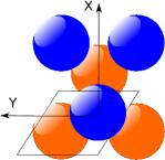
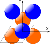
Figure 1: Unit cell of a hcp solid with two different choices of the coordinate system. In both cases the z-axis points out of the plane.

According to the picking rules given in Table 1 there will be only positive $m$-values if the xz-plane is a mirror plane (left), while there will be positive, even and negative, odd $m$-values if the yz-plane is a mirror plane (right). This is confirmed by Table 2 that gives the allowed $(l,m)$-values for an expansion of the potential according to Eq. (86) for this two equivalent descriptions of the system.

	$l$	$0$	$2$	$3$	$4$	$5$	$6$	$7$	$8$
$\sigma_{y}$	$m$	$0$	$0$	$+3$	$0$	$+3$	$0$	$+3$	$0$
(xz)							$+6$		$+6$
$\sigma_{x}$	$m$	$0$	$0$	$-3$	$0$	$-3$	$0$	$-3$	$0$
(yz)							$+6$		$+6$

Table 2: Non-vanishing elements $V_{L}(r)$ for the expansion of the potential according to Eq. (86) for the atom shown in Fig. 1 at the origin with the magnetization along the $\hat{z}$ direction given for a maximum angular momentum $l_{max}=8$. The first and second rows give the allowed values for $m$ for the xz- and yz-planes, respectively, being a mirror plane ($\sigma_{y}$ and $\sigma_{x}$, respectively).

Obviously, the non-vanishing potential terms $V_{L}(r)$ determine which potential matrix element functions $V_{\Lambda\,\Lambda^{\prime}}^{\pm}(r)$ are non-zero. These in turn determine which $\Lambda$-channels are coupled in the radial Dirac equations (54) and (73), i.e. which $\Lambda$-channels contribute to the expansion of the RHS and LHS solutions in Eqs. (37) and (58). This information is given by the wave function coupling scheme shown in Fig. 2.

	$s_{1/2}$		$p_{1/2}$		$p_{3/2}$				$d_{3/2}$				$d_{5/2}$
$s_{1/2}$	A									A					A
		B									B					B
$p_{1/2}$			C			C												C
				D			D						D
					E							E					E
$p_{3/2}$			C			C												C
				D			D						D
								F	F					F
								F	F					F
$d_{3/2}$	A									A					A
		B									B					B
					E							E					E
				D			D						D
								F	F					F
$d_{5/2}$	A									A					A
		B									B					B
					E							E					E
			C			C												C

Figure 2: Wave function coupling scheme for the atom shown in Fig. 1 at the origin with the magnetization along the $\hat{z}$ direction in the spin angular representation, i.e. the rows and columns are indexed with $\Lambda=(\kappa,\mu)$ given for a maximum angular momentum $l_{max}=2$. The sub-blocks denoted by $s_{1/2}$ and so on correspond to $\kappa=+1,\,-1,\,+2,\,-2$ and $+3$. Within each sub-block the magnetic quantum number $\mu$ runs from $-j$ to $+j$ with $j=|\kappa|-1/2$. For each column the occurring letter indicates the non-vanishing contributions $\phi_{\Lambda^{\prime}\Lambda}(\mathbf{r},z)$ to the sum $\sum_{\Lambda^{\prime}}\,\phi_{\Lambda^{\prime}\Lambda}(\mathbf{r},z)$. All columns having the same letter contribute to a corresponding sub-block of the t-matrix.

Each letter within a column ($\Lambda$) indicates a contribution $\phi_{\Lambda^{\prime}\Lambda}(\mathbf{r},z)$ to the wave function expansion. Columns with the same letter have the same coupling sequence. In case of regular functions these solutions contribute to a common sub-block of the t-matrix.

V Summary

The full potential version of relativistic multiple scattering theory has been reviewed in detail and an extension to the case of a non-local but site-diagonal complex self-energy $\Sigma(\mathbf{r},\mathbf{r}\,^{\prime},z)$ has been discussed. The properties of the right- (RHS) and left-hand side (LHS) solutions to the corresponding single-site problem have been worked out. It was demonstrated that the presence of a non-local self-energy has far reaching consequences for the construction of the associated single-site Green function. In particular, it turned out that a simple product representation of the single-site Green function in terms of the RHS and LHS solutions can be given only if the self-energy $\Sigma(\mathbf{r},\mathbf{r}\,^{\prime},z)$ can be written as a product of suitable basis functions w.r.t. its dependence on the spatial variables $\mathbf{r}$ and $\mathbf{r}\,^{\prime}$. Furthermore, it was shown that in contrast to the single-site Green function the back-scattering Green function representing the effect of the environment can still be expressed as a product of RHS and LHS solutions as in the case of a local potential. Finally, some practical aspects of relativistic calculations for a general potential have been discussed. In particular the use of symmetry when dealing with the coupled radial equations for the RHS and LHS solutions has been demonstrated.

Appendix A Product representation of the single site Green function

In the following, we consider first the single site Green function $G(\mathbf{r},\mathbf{r}\,^{\prime},z)$ for the case of a general but local potential $V(\mathbf{r})$, i.e. $\Sigma(\mathbf{r},\mathbf{r}\,^{\prime},z)=0$ will be assumed. Butler et al. BGZ92 showed for the corresponding non-relativistic case that the product representation for $G(\mathbf{r},\mathbf{r}\,^{\prime},z)$ as given by Eq. (III.6) is indeed a proper solution for the corresponding defining Eq. (II) for any $\mathbf{r}$ and $\mathbf{r}\,^{\prime}$. For the relativistic case, this proof can be given in an analogous way, as it is shown in the following. To simplify notation the energy argument $z$ will be omitted throughout and the frequent factor $-i\bar{p}$ will be combined with the Hankel function (i.e., $-i\bar{p}h_{\Lambda}(\mathbf{r})\rightarrow h_{\Lambda}(\mathbf{r})$) and correspondingly with all other irregular functions ($H_{\Lambda}(\mathbf{r})$ and $F_{\Lambda}(\mathbf{r})$) used below. In contrast to the non-relativistic case, the RHS and LHS solutions to the Dirac equations have to be distinguished properly, with all quantities referring to the LHS solution indicated by “$\times$”.

Following the scheme of Butler et al. BGZ92 we introduce an alternative RHS solution $\phi_{\Lambda}(\mathbf{r})$ to the Dirac equation (III.1) by imposing the boundary condition

$$\phi_{\Lambda}(\mathbf{r})\rightarrow j_{\Lambda}(\mathbf{r})\qquad\text{for}\qquad\mathbf{r}\rightarrow 0\;.$$

Setting up the Lippmann-Schwinger equation for $\phi_{\Lambda}(\mathbf{r})$ that accounts for that asymptotic behavior one may express it in terms of the Bessel and Hankel functions $j_{\Lambda}(\mathbf{r})$ and $h_{\Lambda}(\mathbf{r})$, respectively, as:

$$\phi_{\Lambda}(\mathbf{r})=\sum\limits_{\Lambda^{\prime}}\,j_{\Lambda^{\prime}}(\mathbf{r})\,C_{\Lambda^{\prime}\Lambda}(r)+h_{\Lambda^{\prime}}(\mathbf{r})\,S_{\Lambda^{\prime}\Lambda}(r)$$ (255)

with the expansion coefficients:

$$C_{\Lambda^{\prime}\Lambda}(r)= \delta_{\Lambda^{\prime}\Lambda} -\int\limits_{0}^{r}d^{3}r\,^{\prime}h_{\Lambda^{\prime}}^{\times}(\mathbf{r}\,^{\prime})\,V(\mathbf{r}\,^{\prime})\,\phi_{\Lambda}(\mathbf{r}\,^{\prime})$$

$$= \,\,C_{\Lambda^{\prime}\Lambda}(r_{\rm crit})\,\, +\int\limits_{r}^{r_{\rm crit}}d^{3}r\,^{\prime}h_{\Lambda^{\prime}}^{\times}(\mathbf{r}\,^{\prime})\,V(\mathbf{r}\,^{\prime})\,\phi_{\Lambda}(\mathbf{r}\,^{\prime})$$

$$S_{\Lambda^{\prime}\Lambda}(r)= \int\limits_{0}^{r}d^{3}r\,^{\prime}j_{\Lambda^{\prime}}^{\times}(\mathbf{r}\,^{\prime})\,V(\mathbf{r}\,^{\prime})\,\phi_{\Lambda}(\mathbf{r}\,^{\prime})$$

and a corresponding expansion for the LHS regular solution $\phi_{\Lambda}^{\times}(\mathbf{r})$:

$$\phi_{\Lambda}^{\times}(\mathbf{r})=\sum\limits_{\Lambda^{\prime}}\,C_{\Lambda\Lambda^{\prime}}^{\times}(r)\,j_{\Lambda^{\prime}}^{\times}(\mathbf{r})+S_{\Lambda\Lambda^{\prime}}^{\times}(r)\,h_{\Lambda^{\prime}}^{\times}(\mathbf{r})$$ (256)

with

$$C_{\Lambda\Lambda^{\prime}}^{\times}(r)= \delta_{\Lambda\Lambda^{\prime}} -\int\limits_{0}^{r}d^{3}r\,^{\prime}\phi_{\Lambda}^{\times}(\mathbf{r}\,^{\prime})\,V(\mathbf{r}\,^{\prime})\,h_{\Lambda^{\prime}}(\mathbf{r}\,^{\prime})$$

$$= \,\,C_{\Lambda^{\prime}\Lambda}^{\times}(r_{\rm crit})\,\, +\int\limits_{r}^{r_{\rm crit}}d^{3}r\,^{\prime}\phi_{\Lambda}^{\times}(\mathbf{r}\,^{\prime})\,V(\mathbf{r}\,^{\prime})\,h_{\Lambda^{\prime}}(\mathbf{r}\,^{\prime})$$

$$S_{\Lambda\Lambda^{\prime}}^{\times}(r)= \int\limits_{0}^{r}d^{3}r\,^{\prime}\phi_{\Lambda}^{\times}(\mathbf{r}\,^{\prime})\,V(\mathbf{r}\,^{\prime})\,j_{\Lambda^{\prime}}(\mathbf{r}\,^{\prime})\;.$$

It should be mentioned that the expansion used here is completely equivalent to that in terms of the Bessel and von Neumann functions used in context of the variable-phase approach of Calogero with the expansion coefficients $C_{\Lambda^{\prime}\Lambda}(r)$ and $S_{\Lambda^{\prime}\Lambda}(r)$ redefined (see section IV.3).

Considering the behavior of these functions for $r>r_{\rm crit}$ one finds the connection to the regular functions $R_{\Lambda}(\mathbf{r})$ and $R_{\Lambda}^{\times}(\mathbf{r})$ introduced in Eqs.(111) and (113), respectively:

$$R_{\Lambda}(\mathbf{r}) = \sum\limits_{\Lambda^{\prime}}\,\phi_{\Lambda^{\prime}}(\mathbf{r})\,C_{\Lambda\Lambda^{\prime}}^{-1}(r)$$ (257)

$$R_{\Lambda}^{\times}(\mathbf{r}) = \sum\limits_{\Lambda^{\prime}}\,C_{\Lambda\Lambda^{\prime}}^{\times-1}(r)\,\phi_{\Lambda^{\prime}}^{\times}(\mathbf{r})$$ (258)

as well as an expression for the $t$-matrix in terms of the expansion coefficients for $r>r_{\rm crit}$:

$$t_{\Lambda^{\prime}\Lambda^{\prime\prime}} = \sum\limits_{\Lambda}\,S_{\Lambda^{\prime}\Lambda}(r_{\rm crit})\,C_{\Lambda\Lambda^{\prime\prime}}^{-1}(r_{\rm crit})$$ (259)

$$t_{\Lambda^{\prime\prime}\Lambda^{\prime}} = \sum\limits_{\Lambda}\,C_{\Lambda^{\prime\prime}\Lambda}^{\times-1}(r_{\rm crit})\,S_{\Lambda\Lambda^{\prime}}^{\times}(r_{\rm crit})\;.$$ (260)

Replacing the regular function $R_{\Lambda}(\mathbf{r})$ ($R_{\Lambda}^{\times}(\mathbf{r})$) in Eq. (III.6) for the Green function by $\phi_{\Lambda}(\mathbf{r})$ ($\phi_{\Lambda}^{\times}(\mathbf{r})$) via Eqs.  (257) and (258) implies a corresponding replacement of the irregular function $H_{\Lambda}^{\times}(\mathbf{r})$ ($H_{\Lambda}(\mathbf{r})$) by its counterpart $F_{\Lambda}^{\times}(\mathbf{r})$ ($F_{\Lambda}(\mathbf{r})$) defined by

$$F_{\Lambda^{\prime}}(\mathbf{r}) = \sum\limits_{\Lambda}\,H_{\Lambda}(\mathbf{r})\,C_{\Lambda\Lambda^{\prime}}^{\times-1}(r)$$ (261)

$$F_{\Lambda^{\prime}}^{\times}(\mathbf{r}) = \sum\limits_{\Lambda}\,C_{\Lambda^{\prime}\Lambda}^{-1}(r)\,H_{\Lambda}^{\times}(\mathbf{r})\;.$$ (262)

Again an expansion of these functions in terms of $j_{\Lambda}(\mathbf{r})$ and $h_{\Lambda}(\mathbf{r})$ can be given starting from the corresponding Lippmann-Schwinger equation and imposing the appropriate boundary conditions:

$$F_{\Lambda}(\mathbf{r})=\sum\limits_{\Lambda^{\prime}}\,j_{\Lambda^{\prime}}(\mathbf{r})\,\bar{C}_{\Lambda^{\prime}\Lambda}(r)+h_{\Lambda^{\prime}}(\mathbf{r})\,\bar{S}_{\Lambda^{\prime}\Lambda}(r)$$ (263)

with

$$\bar{C}_{\Lambda^{\prime}\Lambda}(r)= \int\limits_{r}^{r_{\rm crit}}d^{3}r\,^{\prime}h_{\Lambda^{\prime}}^{\times}(\mathbf{r}\,^{\prime})\,V(\mathbf{r}\,^{\prime})\,F_{\Lambda}(\mathbf{r}\,^{\prime})$$

$$\bar{S}_{\Lambda^{\prime}\Lambda}(r)= \,\,C_{\Lambda^{\prime}\Lambda}^{\times-1}(r_{\rm crit})\,\, -\int\limits_{r}^{r_{\rm crit}}d^{3}r\,^{\prime}j_{\Lambda^{\prime}}^{\times}(\mathbf{r}\,^{\prime})\,V(\mathbf{r}\,^{\prime})\,F_{\Lambda}(\mathbf{r}\,^{\prime})$$

$$F_{\Lambda}^{\times}(\mathbf{r})=\sum\limits_{\Lambda^{\prime}}\,\bar{C}_{\Lambda\Lambda^{\prime}}^{\times}(r)\,j_{\Lambda^{\prime}}^{\times}(\mathbf{r})+\bar{S}_{\Lambda\Lambda^{\prime}}^{\times}(r)\,h_{\Lambda^{\prime}}^{\times}(\mathbf{r})$$ (264)

with

$$\bar{C}_{\Lambda\Lambda^{\prime}}^{\times}(r)= \int\limits_{r}^{r_{\rm crit}}d^{3}r\,^{\prime}F_{\Lambda}^{\times}(\mathbf{r}\,^{\prime})\,V(\mathbf{r}\,^{\prime})\,h_{\Lambda^{\prime}}(\mathbf{r}\,^{\prime})$$

$$\bar{S}_{\Lambda\Lambda^{\prime}}^{\times}(r)= \,\,C_{\Lambda\Lambda^{\prime}}^{-1}(r_{\rm crit})\,\, -\int\limits_{r}^{r_{\rm crit}}d^{3}r\,^{\prime}F_{\Lambda}^{\times}(\mathbf{r}\,^{\prime})\,V(\mathbf{r}\,^{\prime})\,j_{\Lambda^{\prime}}(\mathbf{r}\,^{\prime})\;.$$

Inserting now the expansion given in Eqs.  (255), (256), (263) and (264) into the expression for the Green function

$$G(\mathbf{r},\mathbf{r}\,^{\prime})=\sum\limits_{\Lambda} \phi_{\Lambda}(\mathbf{r})\,F_{\Lambda}^{\times}(\mathbf{r}\,^{\prime})\,\theta(r^{\prime}-r)$$

$$+ F_{\Lambda}(\mathbf{r})\phi_{\Lambda}^{\times}(\mathbf{r}\,^{\prime})\,\theta(r-r^{\prime})$$ (265)

one is led to a corresponding expansion for the Green function in terms of $j_{\Lambda}(\mathbf{r})$ and $h_{\Lambda}(\mathbf{r})$:

$$G(\mathbf{r},\mathbf{r}\,^{\prime})=\sum\limits_{\Lambda^{\prime\prime}\Lambda^{\prime\prime\prime}} \Bigg{\{} j_{\Lambda^{\prime\prime}}(\mathbf{r})\,\Bigg{[}\sum\limits_{\Lambda}C_{\Lambda^{\prime\prime}\Lambda}(r)\bar{C}_{\Lambda\Lambda^{\prime\prime\prime}}^{\times}(r^{\prime})\Bigg{]}j_{\Lambda^{\prime\prime\prime}}^{\times}(\mathbf{r}\,^{\prime})$$

$$+ j_{\Lambda^{\prime\prime}}(\mathbf{r})\,\Bigg{[}\sum\limits_{\Lambda}C_{\Lambda^{\prime\prime}\Lambda}(r)\bar{S}_{\Lambda\Lambda^{\prime\prime\prime}}^{\times}(r^{\prime})\Bigg{]}h_{\Lambda^{\prime\prime\prime}}^{\times}(\mathbf{r}\,^{\prime})$$

$$+ h_{\Lambda^{\prime\prime}}(\mathbf{r})\,\Bigg{[}\sum\limits_{\Lambda}S_{\Lambda^{\prime\prime}\Lambda}(r)\bar{C}_{\Lambda\Lambda^{\prime\prime\prime}}^{\times}(r^{\prime})\Bigg{]}j_{\Lambda^{\prime\prime\prime}}^{\times}(\mathbf{r}\,^{\prime})$$

$$+ h_{\Lambda^{\prime\prime}}(\mathbf{r})\,\Bigg{[}\sum\limits_{\Lambda}S_{\Lambda^{\prime\prime}\Lambda}(r)\bar{S}_{\Lambda\Lambda^{\prime\prime\prime}}^{\times}(r^{\prime})\Bigg{]}h_{\Lambda^{\prime\prime\prime}}^{\times}(\mathbf{r}\,^{\prime})\Bigg{\}}$$

$$\times \theta(r^{\prime}\!\!-\!r)$$

$$+\sum\limits_{\Lambda^{\prime\prime}\Lambda^{\prime\prime\prime}} \Bigg{\{} j_{\Lambda^{\prime\prime}}(\mathbf{r})\,\Bigg{[}\sum\limits_{\Lambda}\bar{C}_{\Lambda^{\prime\prime}\Lambda}(r)\,C_{\Lambda\Lambda^{\prime\prime\prime}}^{\times}(r^{\prime})\Bigg{]}j_{\Lambda^{\prime\prime\prime}}^{\times}(\mathbf{r}\,^{\prime})$$ (266)

$$+ j_{\Lambda^{\prime\prime}}(\mathbf{r})\,\Bigg{[}\sum\limits_{\Lambda}\bar{C}_{\Lambda^{\prime\prime}\Lambda}(r)\,S_{\Lambda\Lambda^{\prime\prime\prime}}^{\times}(r^{\prime})\Bigg{]}h_{\Lambda^{\prime\prime\prime}}^{\times}(\mathbf{r}\,^{\prime})$$

$$+ h_{\Lambda^{\prime\prime}}(\mathbf{r})\,\Bigg{[}\sum\limits_{\Lambda}\bar{S}_{\Lambda^{\prime\prime}\Lambda}(r)\,C_{\Lambda\Lambda^{\prime\prime\prime}}^{\times}(r^{\prime})\Bigg{]}j_{\Lambda^{\prime\prime\prime}}^{\times}(\mathbf{r}\,^{\prime})$$

$$+ h_{\Lambda^{\prime\prime}}(\mathbf{r})\,\Bigg{[}\sum\limits_{\Lambda}\bar{S}_{\Lambda^{\prime\prime}\Lambda}(r)\,S_{\Lambda\Lambda^{\prime\prime\prime}}^{\times}(r^{\prime})\Bigg{]}h_{\Lambda^{\prime\prime\prime}}^{\times}(\mathbf{r}\,^{\prime})\Bigg{\}}$$

$$\times \theta(r\!\!-\!r^{\prime})\;.$$

To evaluate these expressions it is helpful to use in addition the following Lippmann-Schwinger equations

$$R_{\Lambda}(\mathbf{r})=j_{\Lambda}(\mathbf{r})+\int\limits_{0}^{r_{\rm crit}}d^{3}r^{\prime}\,G(\mathbf{r},\mathbf{r}\,^{\prime})\,V(\mathbf{r}\,^{\prime})\,j_{\Lambda}(\mathbf{r}\,^{\prime})\$$

$$F_{\Lambda}(\mathbf{r})=h_{\Lambda}(\mathbf{r})+\int\limits_{0}^{r_{\rm crit}}d^{3}r^{\prime}\,G(\mathbf{r}\,^{\prime},\mathbf{r})\,V(\mathbf{r}\,^{\prime})\,h_{\Lambda}(\mathbf{r}\,^{\prime})$$

as well as their counterparts for the LHS solutions $R_{\Lambda}^{\times}(\mathbf{r})$ and $F_{\Lambda}^{\times}(\mathbf{r})$ together with the relation for the $t$-matrix operator

$$\hat{t}=\hat{V}+\hat{V}\,\hat{G}\,\hat{V}.$$ (267)

The sums […] in Eq. (A) can now be reformulated more or less the same way as sketched in the appendix of Ref. BGZ92, for the non-relativistic case, however, taking the difference between RHS and LHS solutions into account. This way one can express the various sums […] in Eq. (A) in terms of the real space representation of the $t$-matrix operator

$$\sum\limits_{\Lambda^{\prime\prime}}C_{\Lambda\Lambda^{\prime\prime}}(r)\,\bar{C}_{\Lambda^{\prime\prime}\Lambda^{\prime}}^{\times}(r^{\prime})=\sum\limits_{\Lambda^{\prime\prime}}\bar{C}_{\Lambda\Lambda^{\prime\prime}}(r)\,C_{\Lambda^{\prime\prime}\Lambda^{\prime}}^{\times}(r^{\prime}) =\int\limits_{r}^{r_{\rm crit}}d^{3}r_{1}\int\limits_{r^{\prime}}^{r_{\rm crit}}d^{3}r_{2}\,h_{\Lambda}^{\times}(\mathbf{r}_{1})\,t(\mathbf{r}_{1},\mathbf{r}_{2})\,h_{\Lambda^{\prime}}(\mathbf{r}_{2}) =G_{\Lambda\Lambda^{\prime}}^{jj}(r,r^{\prime})$$ (268)

$$\sum\limits_{\Lambda^{\prime\prime}}C_{\Lambda\Lambda^{\prime\prime}}(r)\,\bar{S}_{\Lambda^{\prime\prime}\Lambda^{\prime}}^{\times}(r^{\prime})=\sum\limits_{\Lambda^{\prime\prime}}\bar{C}_{\Lambda\Lambda^{\prime\prime}}(r)\,S_{\Lambda^{\prime\prime}\Lambda^{\prime}}^{\times}(r^{\prime}) =\int\limits_{r}^{r_{\rm crit}}d^{3}r_{1}\int\limits_{0}^{r^{\prime}}d^{3}r_{2}\,h_{\Lambda}^{\times}(\mathbf{r}_{1})\,t(\mathbf{r}_{1},\mathbf{r}_{2})\,j_{\Lambda^{\prime}}(\mathbf{r}_{2})$$ (269)

$$+\,\,\delta_{\Lambda\Lambda^{\prime}}\,\theta(r^{\prime}-r) =G_{\Lambda\Lambda^{\prime}}^{jh}(r,r^{\prime})$$

$$\sum\limits_{\Lambda^{\prime\prime}}S_{\Lambda\Lambda^{\prime\prime}}(r)\,\bar{C}_{\Lambda^{\prime\prime}\Lambda^{\prime}}^{\times}(r^{\prime})=\sum\limits_{\Lambda^{\prime\prime}}\bar{S}_{\Lambda\Lambda^{\prime\prime}}(r)\,C_{\Lambda^{\prime\prime}\Lambda^{\prime}}^{\times}(r^{\prime}) =\int\limits_{0}^{r}d^{3}r_{1}\int\limits_{r^{\prime}}^{r_{\rm crit}}d^{3}r_{2}\,j_{\Lambda}^{\times}(\mathbf{r}_{1})\,t(\mathbf{r}_{1},\mathbf{r}_{2})\,h_{\Lambda^{\prime}}(\mathbf{r}_{2})$$ (270)

$$+\,\,\delta_{\Lambda\Lambda^{\prime}}\,\theta(r-r^{\prime}) =G_{\Lambda\Lambda^{\prime}}^{hj}(r,r^{\prime})$$

$$\sum\limits_{\Lambda^{\prime\prime}}S_{\Lambda\Lambda^{\prime\prime}}(r)\,\bar{S}_{\Lambda^{\prime\prime}\Lambda^{\prime}}^{\times}(r^{\prime})=\sum\limits_{\Lambda^{\prime\prime}}\bar{S}_{\Lambda\Lambda^{\prime\prime}}(r)\,S_{\Lambda^{\prime\prime}\Lambda^{\prime}}^{\times}(r^{\prime}) =\int\limits_{0}^{r}d^{3}r_{1}\int\limits_{0}^{r^{\prime}}d^{3}r_{2}\,j_{\Lambda}^{\times}(\mathbf{r}_{1})\,t(\mathbf{r}_{1},\mathbf{r}_{2})\,j_{\Lambda^{\prime}}(\mathbf{r}_{2}) =G_{\Lambda\Lambda^{\prime}}^{hh}(r,r^{\prime})\;.$$ (271)

This result is exactly what has to be expected on the basis of the representation of the Green function $G(\mathbf{r},\mathbf{r}\,^{\prime})$ in terms of the $t$-matrix and the free electron Green function $G^{0}(\mathbf{r},\mathbf{r}\,^{\prime})$ as given in Eq. (108). Inserting the explicit expression for $G^{0}(\mathbf{r},\mathbf{r}\,^{\prime})$ in terms of the Bessel and Hankel functions (see Eq. (93)) into Eq. (108) one is led to the expression for the Green function $G(\mathbf{r},\mathbf{r}\,^{\prime})$ in terms of $j_{\Lambda}(\mathbf{r})$ and $h_{\Lambda}(\mathbf{r})$ with the expansion coefficients given by the integrals as listed in Eqs.  (268) to (271). This direct derivation of the integral form of the expansion coefficients $G_{\Lambda\Lambda^{\prime}}^{\alpha\beta}(r,r^{\prime})$ ($\alpha,\,\beta=j,\,h$) does obviously not depend on the specific form of the potential. For that reason these expressions have to hold also for the more general situation of a non-local potential (see below).

The expansion of the Green function given by Eq. (A) allows now straight forwardly to demonstrate that Eq. (II) is solved for any $\mathbf{r}$ and $\mathbf{r}\,^{\prime}$. For $\mathbf{r}\neq\mathbf{r}\,^{\prime}$ this is ensured by constructing $G(\mathbf{r},\mathbf{r}\,^{\prime})$ in terms of RHS and LHS solutions to the corresponding Dirac equations. For $\mathbf{r}=\mathbf{r}\,^{\prime}$ the inhomogeneity represented by the $\delta$-function has to be recovered in addition. To demonstrate this one integrates Eq. (II) w.r.t. $r$ over the interval $[r^{\prime}-\epsilon,r^{\prime}+\epsilon]$ and takes the limit $\epsilon\rightarrow 0$ afterwards. For this purpose it is advantageous to split the Dirac Hamiltonian in Eq. (III.1) into the term involving the radial derivative $\hat{\cal H}_{\rm rad}(\mathbf{r})=-ic\,\alpha_{r}\frac{\partial}{\partial r}$ and the remaining rest $\hat{\cal H}_{\rm rest}(\mathbf{r})=\hat{\cal H}(\mathbf{r})-\hat{\cal H}_{\rm rad}(\mathbf{r})$. Here we combined $\gamma_{s}\,\sigma_{r}$ used in Eq. (6) to $-\alpha_{r}=-\mathbf{\alpha}\cdot\mathbf{r}/r$ Ros61 . With this one has:

$$-\int\limits_{r^{\prime}-\epsilon}^{r^{\prime}+\epsilon}dr\,\hat{\cal H}_{\rm rad}(\mathbf{r})\,G(\mathbf{r},\mathbf{r}\,^{\prime})+\int\limits_{r^{\prime}-\epsilon}^{r^{\prime}+\epsilon}dr\,\Big{(}z-\hat{\cal H}_{\rm rest}(\mathbf{r})\Big{)}G(\mathbf{r},\mathbf{r}\,^{\prime})=\int\limits_{r^{\prime}-\epsilon}^{r^{\prime}+\epsilon}dr\,\delta(\mathbf{r}-\mathbf{r}\,^{\prime}){{1}}_{4}\;.$$

As $G(\mathbf{r},\mathbf{r}\,^{\prime})$ is continuous at $r=r^{\prime}$ w.r.t. $r$ the second integral will vanish for $\epsilon\rightarrow 0$. Using the relation $\delta(\mathbf{r}-\mathbf{r}\,^{\prime})=\frac{1}{r^{2}}\,\delta(r-r^{\prime})\,\delta(\hat{r},\hat{r}^{\prime})$ for the $\delta$-function one gets

$$-\!\!\int\limits_{r^{\prime}-\epsilon}^{r^{\prime}+\epsilon}\!\!dr\Big{(}-ic\,\alpha_{r}\frac{\partial}{\partial r}\Big{)}\,G(\mathbf{r},\mathbf{r}\,^{\prime})=\!\!\int\limits_{r^{\prime}-\epsilon}^{r^{\prime}+\epsilon}\!\!dr\,\frac{1}{r^{2}}\delta(r-r\,^{\prime})\delta(\hat{r},\hat{r}^{\prime}){{1}}_{4}$$

$$-ic\,\alpha_{r}\Big{[}G(\mathbf{r}\,^{\prime}+\epsilon,\mathbf{r}\,^{\prime})-G(\mathbf{r}\,^{\prime}-\epsilon,\mathbf{r}\,^{\prime})\Big{]}=\frac{1}{r^{\prime 2}}\,\delta(\hat{r},\hat{r}^{\prime}){{1}}_{4}\;.$$

Inserting now the expansion of $G(\mathbf{r},\mathbf{r}\,^{\prime})$ in terms of $j_{\Lambda}$ and $h_{\Lambda}$ as given by Eq. (A) and making use of Eqs. (268) to (271) one is led in the limit $\epsilon\rightarrow 0$ to:

$$-ic\,\alpha_{r}\sum\limits_{\Lambda}\Big{(}j_{\Lambda}(\mathbf{r})h_{\Lambda}^{\times}(\mathbf{r}\,^{\prime})-h_{\Lambda}(\mathbf{r})j_{\Lambda}^{\times}(\mathbf{r}\,^{\prime})\Big{)}=\frac{1}{r^{\prime 2}}\,\delta(\hat{r},\hat{r}^{\prime}){{1}}_{4}\;.$$

The expression on the left hand side can be evaluated straight forwardly using the definition of $\alpha_{r}$ together with Eq. (41). Finally, making use of the Wronskian of the Bessel and Hankel functions (with the later ones including in this section the factor $-i\bar{p}$) given by Eq. (149) together with the relations

$$\sum\limits_{\Lambda}\chi_{\Lambda}(\hat{r})\,\chi_{\Lambda}^{\dagger}(\hat{r}^{\prime})=\sum\limits_{\Lambda}\chi_{-\Lambda}(\hat{r})\,\chi_{-\Lambda}^{\dagger}(\hat{r}^{\prime})=\delta(\hat{r},\hat{r}^{\prime}){{1}}_{2}$$

the equivalency of the left and right hand side of Eq. (A) can be demonstrated completing the proof this way.

To investigate whether the product representation of $G(\mathbf{r},\mathbf{r}\,^{\prime})$ given by Eq. (III.6) is also a proper solution for the defining Eq. (II) for a non-local potential ${\cal V}(\mathbf{r},\mathbf{r}\,^{\prime})=V(\mathbf{r})\,\delta(\mathbf{r}-\mathbf{r}\,^{\prime})+\Sigma(\mathbf{r},\mathbf{r}\,^{\prime})$ one may generalize the expansion of the various wave functions in terms of $j_{\Lambda}(\mathbf{r})$ and $h_{\Lambda}(\mathbf{r})$ in an appropriate way. For example for the expansion coefficient $C_{\Lambda^{\prime}\Lambda}(r)$ of $\phi_{\Lambda}(\mathbf{r})$ in Eq. (255) one gets:

$$C_{\Lambda^{\prime}\Lambda}(r)=\delta_{\Lambda\Lambda^{\prime}}-\int\limits_{0}^{r}d^{3}r^{\prime}h_{\Lambda^{\prime}}^{\times}(\mathbf{r}\,^{\prime})\int\limits_{0}^{r_{\rm crit}}d^{3}r^{\prime\prime}{\cal V}(\mathbf{r}\,^{\prime},\mathbf{r}\,^{\prime\prime})\,\phi_{\Lambda}(\mathbf{r}\,^{\prime\prime})\;.$$

Considering now for example the case $r^{\prime}>r$, this together with a corresponding expression for $\bar{C}_{\Lambda^{\prime}\Lambda}^{\times}(r)$ leads to:

$$\sum\limits_{\Lambda^{\prime\prime}}C_{\Lambda\Lambda^{\prime\prime}}(r)\,\bar{C}_{\Lambda^{\prime\prime}\Lambda^{\prime}}^{\times}(r^{\prime}) = \sum\limits_{\Lambda^{\prime\prime}}\Bigg{[}\delta_{\Lambda^{\prime\prime}\Lambda}-\int\limits_{0}^{r}d^{3}r_{1}\,h_{\Lambda}^{\times}(\mathbf{r}_{1})\int\limits_{0}^{r_{\rm crit}}d^{3}r_{2}{\cal V}(\mathbf{r}_{1},\mathbf{r}_{2})\phi_{\Lambda^{\prime\prime}}(\mathbf{r}_{2})\Bigg{]}\,$$

$$\qquad\qquad\Bigg{[}\int\limits_{r^{\prime}}^{r_{\rm crit}}d^{3}r_{3},F_{\Lambda^{\prime\prime}}^{\times}(\mathbf{r}_{3})\!\!\int\limits_{0}^{r_{\rm crit}}d^{3}r_{4}{\cal V}(\mathbf{r}_{3},\mathbf{r}_{4})h_{\Lambda^{\prime}}(\mathbf{r}_{4})\Bigg{]}\;.$$

In contrast to the case of a local potential $V(\mathbf{r})$ the restriction $r_{3}\geq r^{\prime}>r\geq r_{2}$ does not hold anymore. As a consequence the combined term $\sum\limits_{\Lambda^{\prime\prime}}\phi_{\Lambda^{\prime\prime}}(\mathbf{r}_{2})F_{\Lambda^{\prime\prime}}^{\times}(\mathbf{r}_{3})$ cannot be identified with the Green function $G(\mathbf{r}_{2},\mathbf{r}_{3})$ anymore. Due to this, the sum $\sum\limits_{\Lambda^{\prime\prime}}C_{\Lambda\Lambda^{\prime\prime}}(r)\,\bar{C}_{\Lambda^{\prime\prime}\Lambda^{\prime}}^{\times}(r^{\prime})$ is not identical to the integral $\int\limits_{r}^{r_{\rm crit}}d^{3}r_{1}\int\limits_{r^{\prime}}^{r_{\rm crit}}d^{3}r_{2}\,h_{\Lambda}^{\times}(\mathbf{r}_{1})\,t(\mathbf{r}_{1},\mathbf{r}_{2})\,h_{\Lambda^{\prime}}(\mathbf{r}_{2})$. As this is required also for the case of a non-local potential (see above) the product representation for the Green function given in Eq. (A) cannot be valid in case of a non-local potential. This obviously also applies if an expansion of the self-energy in terms of basis functions as given by Eq. (23) is assumed. In this case the double integral over $\mathbf{r}_{1}$ and $\mathbf{r}_{2}$ and also that over $\mathbf{r}_{3}$ and$\mathbf{r}_{4}$ factorize, but the above mentioned necessary restriction concerning $r_{2}$ and $r_{3}$ still does not hold.

- (1) E. Roman, Y. Mokrousov, and I. Souza, Phys. Rev. Lett. 103(9), 097203 (2009), URL http://link.aps.org/doi/10.1103/PhysRevLett.103.097203.
- (2) S. Lowitzer, M. Gradhand, D. Ködderitzsch, D. V. Fedorov, I. Mertig, and H. Ebert, Phys. Rev. Lett. 106(5), 056601 (2011), URL http://link.aps.org/doi/10.1103/PhysRevLett.106.056601.
- (3) K. Tauber, M. Gradhand, D. V. Fedorov, and I. Mertig, Phys. Rev. Lett. 109, 026601 (2012), URL http://link.aps.org/doi/10.1103/PhysRevLett.109.026601.
- (4) B. Zimmermann, K. Chadova, D. Ködderitzsch, S. Blügel, H. Ebert, D. V. Fedorov, N. H. Long, P. Mavropoulos, I. Mertig, Y. Mokrousov, and M. Gradhand, Phys. Rev. B 90, 220403 (2014), URL http://link.aps.org/doi/10.1103/PhysRevB.90.220403.
- (5) H. Ebert, Rep. Prog. Phys. 59(12), 1665 (1996), URL http://stacks.iop.org/0034-4885/59/i=12/a=003.
- (6) T. Huhne and H. Ebert, Europhys. Lett. 59(4), 612 (2002), URL http://stacks.iop.org/0295-5075/59/i=4/a=612.
- (7) A. Vernes, I. Reichl, P. Weinberger, L. Szunyogh, and C. Sommers, Phys. Rev. B 70(19), 195407 (2004), ISSN 0163-1829, URL http://dx.doi.org/10.1103/PhysRevB.70.195407.
- (8) C. R. Ast, D. Pacile, L. Moreschini, M. C. Falub, M. Papagno, K. Kern, M. Grioni, J. Henk, A. Ernst, S. Ostanin, and P. Bruno, Phys. Rev. B 77(8), 081407 (2008), ISSN 1098-0121, URL http://dx.doi.org/10.1103/PhysRevB.77.081407.
- (9) J. Braun, K. Miyamoto, A. Kimura, T. Okuda, M. Donath, H. Ebert, and J. Minár, New Journal of Physics 16(1), 015005 (2014), URL http://stacks.iop.org/1367-2630/16/i=1/a=015005.
- (10) M. Z. Hasan and C. L. Kane, Rev. Mod. Phys. 82(4), 3045 (2010), URL http://link.aps.org/doi/10.1103/RevModPhys.82.3045.
- (11) X.-L. Qi and S.-C. Zhang, Rev. Mod. Phys. 83, 1057 (2011), URL http://link.aps.org/doi/10.1103/RevModPhys.83.1057.
- (12) H. Ebert, D. Ködderitzsch, and J. Minár, Rep. Prog. Phys. 74(9), 096501 (2011), URL http://stacks.iop.org/0034-4885/74/i=9/a=096501.
- (13) P. Soven, Phys. Rev. 156(3), 809 (1967), URL http://link.aps.org/doi/10.1103/PhysRev.156.809.
- (14) R. Feder, F. Rosicky, and B. Ackermann, Z. Physik B 52, 31 (1983), URL http://dx.doi.org/10.1007/BF01305895.
- (15) P. Strange, J. Staunton, and B. L. Gyorffy, J. Phys. C: Solid State Phys. 17(19), 3355 (1984), ISSN 0022-3719, URL http://dx.doi.org/10.1088/0022-3719/17/19/011.
- (16) H. Ebert and M. Battocletti, Solid State Commun. 98, 785 (1996), URL http://www.sciencedirect.com/science/article/B6TVW-3VR9T62-15/2/52da5f6831b941392e8f11eec2d42002.
- (17) H. Ebert, M. Battocletti, and E. K. U. Gross, Europhys. Lett. 40(5), 545 (1997), URL http://stacks.iop.org/0295-5075/40/i=5/a=545.
- (18) S. Bornemann, J. Minár, J. Braun, D. Ködderitzsch, and H. Ebert, Solid State Commun. 152, 85 (2012), URL http://www.sciencedirect.com/science/article/pii/S0038109811005977.
- (19) E. Tamura, Phys. Rev. B 45(7), 3271 (1992), URL http://link.aps.org/doi/10.1103/PhysRevB.45.3271.
- (20) S. C. Lovatt, B. L. Gyorffy, and G. Y. Guo, J. Phys.: Cond. Mat. 5(43), 8005 (1993), ISSN 0953-8984, URL http://dx.doi.org/10.1088/0953-8984/5/43/014.
- (21) X. Wang, X.-G. Zhang, W. H. Butler, G. M. Stocks, and B. N. Harmon, Phys. Rev. B 46(15), 9352 (1992), URL http://link.aps.org/doi/10.1103/PhysRevB.46.9352.
- (22) T. Huhne, C. Zecha, H. Ebert, P. H. Dederichs, and R. Zeller, Phys. Rev. B 58(16), 10236 (1998), URL http://link.aps.org/doi/10.1103/PhysRevB.58.10236.
- (23) M. E. Rose, Relativistic Electron Theory (Wiley, New York, 1961), URL http://openlibrary.org/works/OL3517103W/Relativistic_electron_theory.
- (24) E. Engel and R. M. Dreizler, Density Functional Theory – An advanced course (Springer, Berlin, 2011), URL http://www.springerlink.com/content/m246q2.
- (25) H. Eschrig, The Fundamentals of Density Functional Theory (B G Teubner Verlagsgesellschaft, Stuttgart, Leipzig, 1996).
- (26) A. H. MacDonald and S. H. Vosko, J. Phys. C: Solid State Phys. 12, 2977 (1979), URL http://iopscience.iop.org/0022-3719/12/15/007.
- (27) M. V. Ramana and A. K. Rajagopal, J. Phys. C: Solid State Phys. 12, L845 (1979).
- (28) A. K. Rajagopal and J. Callaway, Phys. Rev. B 7(5), 1912 (1973), URL http://link.aps.org/doi/10.1103/PhysRevB.7.1912.
- (29) G. Vignale and M. Rasolt, Phys. Rev. Lett. 59(20), 2360 (1987), URL http://link.aps.org/doi/10.1103/PhysRevLett.59.2360.
- (30) G. Diener, J. Phys.: Cond. Mat. 3(47), 9417 (1991), URL http://stacks.iop.org/0953-8984/3/i=47/a=014.
- (31) H. J. F. Jansen, Phys. Rev. B 38(12), 8022 (1988), URL http://link.aps.org/doi/10.1103/PhysRevB.38.8022.
- (32) E. Tamura and R. Feder, Solid State Commun. 58(10), 729 (1986), ISSN 0038-1098, URL http://www.sciencedirect.com/science/article/pii/0038109886905119.
- (33) V. I. Anisimov, J. Zaanen, and O. K. Andersen, Phys. Rev. B 44(3), 943 (1991), URL http://link.aps.org/doi/10.1103/PhysRevB.44.943.
- (34) A. Georges, G. Kotliar, W. Krauth, and M. J. Rozenberg, Rev. Mod. Phys. 68(1), 13 (1996), URL http://link.aps.org/doi/10.1103/RevModPhys.68.13.
- (35) K. Held, Adv. Phys. 56, 829 (2007).
- (36) F. Aryasetiawan and O. Gunnarsson, Rep. Prog. Phys. 61(3), 237 (1998), URL http://stacks.iop.org/0034-4885/61/i=3/a=002.
- (37) W. van Haeringen, B. Farid, and D. Lenstra, Physica Scripta 1987(T19A), 282 (1987), URL http://stacks.iop.org/1402-4896/1987/i=T19A/a=039.
- (38) A. J. Layzer, Phys. Rev. 129, 897 (1963), URL http://link.aps.org/doi/10.1103/PhysRev.129.897.
- (39) C. R. Natoli, P. Krüger, K. Hatada, K. Hayakawa, D. Sébilleau, and O. Šipr, J. Phys.: Cond. Mat. 24(36), 365501 (2012), URL http://stacks.iop.org/0953-8984/24/i=36/a=365501.
- (40) E. Tamura and R. Feder, Solid State Commun. 70(2), 205 (1989), ISSN 0038-1098, URL http://www.sciencedirect.com/science/article/pii/0038109889909757.
- (41) H. Ebert, A. Perlov, and S. Mankovsky, Solid State Commun. 127, 443 (2003), URL http://www.sciencedirect.com/science/article/pii/S0038109803004551.
- (42) J. Minár, L. Chioncel, A. Perlov, H. Ebert, M. I. Katsnelson, and A. I. Lichtenstein, Phys. Rev. B 72, 045125 (2005), URL http://link.aps.org/doi/10.1103/PhysRevB.72.045125.
- (43) P. Weinberger, Electron Scattering Theory for Ordered and Disordered Matter (Oxford University Press, Oxford, 1990).
- (44) A. Gonis, Green functions for ordered and disordered systems (North-Holland, Amsterdam, 1992).
- (45) A. Gonis and W. H. Butler, Multiple scattering in solids, Graduate Texts in Contemporary Physics (Springer, Berlin, 1999), URL http://www.springer.com/materials/book/978-0-387-98853-5.
- (46) Abramowitz and Stegun, Handbook of mathematical functions (1964), URL URL.
- (47) S. Kaprzyk and A. Bansil, Phys. Rev. B 42(12), 7358 (1990), URL http://link.aps.org/doi/10.1103/PhysRevB.42.7358.
- (48) A. F. Tatarchenko and N. I. Kulikov, Phys. Rev. B 50(12), 8266 (1994), URL http://link.aps.org/doi/10.1103/PhysRevB.50.8266.
- (49) R. Zeller, J. Phys.: Cond. Mat. 17(35), 5367 (2005), URL http://stacks.iop.org/0953-8984/17/i=35/a=005.
- (50) It should be noted that the definition for the relativistic Wronskian given here deviates from that of Tamura Tam92 by the factor that is not included in Eq. (145). This definition for the relativistic Wronskian leads in the non-relativistic limit () to its conventional counterpart if the small component is eliminated by means of the radial Dirac equation.
- (51) R. Zeller, private communication (2015).
- (52) J. S. Faulkner and G. M. Stocks, Phys. Rev. B 21(8), 3222 (1980), URL http://link.aps.org/doi/10.1103/PhysRevB.21.3222.
- (53) W. H. Butler, A. Gonis, and X.-G. Zhang, Phys. Rev. B 45(20), 11527 (1992), URL http://link.aps.org/doi/10.1103/PhysRevB.45.11527.
- (54) R. Zeller, P. H. Dederichs, B. Újfalussy, L. Szunyogh, and P. Weinberger, Phys. Rev. B 52(12), 8807 (1995), URL http://link.aps.org/doi/10.1103/PhysRevB.52.8807.
- (55) P. Kordt, Single-Site Green Function of the Dirac Equation for Full-Potential Electron Scattering, Key Technologies, Volume 34, Tech. Rep., Forschungszentrum Jülich GmbH (2012).
- (56) M. Geilhufe, S. Achilles, M. A. Köbis, M. Arnold, I. Mertig, W. Hergert, and A. Ernst, J. Phys.: Cond. Mat. 27(43), 435202 (2015), URL http://stacks.iop.org/0953-8984/27/i=43/a=435202.
- (57) W. H. Press, B. P. Flannery, S. A. Teukolsky, and W. T. Vetterling, The Art of Scientific Computing (Cambridge University Press, London, 1986).
- (58) H. Ebert and B. L. Gyorffy, J. Phys. F: Met. Phys. 18(3), 451 (1988), URL http://stacks.iop.org/0305-4608/18/i=3/a=015.
- (59) F. Calogero, Variable Phase Approach to Potential Scattering (Academic Press, New York, 1967).
- (60) B. Drittler, KKR-Greensche Funktionsmethode fuer das volle Zellpotential, Ph.D. thesis, RWTH Aachen (1990), URL URL.
- (61) M. Ogura and H. Akai, J. Phys.: Cond. Mat. 17(37), 5741 (2005), URL http://stacks.iop.org/0953-8984/17/i=37/a=011.
- (62) K. Kurki-Suonio, Isr. J. Chem. 16, 115 (1977).