Derivation of instanton rate theory from first principles

Abstract

Instanton rate theory is used to study tunneling events in a wide range of systems including low-temperature chemical reactions. Despite many successful applications, the method has never been obtained from first principles, relying instead on the “$\operatorname{Im}F$” premise. In this paper, the same expression for the rate of barrier penetration at finite temperature is rederived from quantum scattering theory [W. H. Miller, S. D. Schwartz, and J. W. Tromp, J. Chem. Phys. 79, 4889 (1983)] using a semiclassical Green’s function formalism. This justifies the instanton approach and provides a route to deriving the rate of other processes.

Nuclear tunneling can significantly affect chemical reactivity Bell (1980); Carpenter (2011); Ley et al. (2012), but the most common theoretical methods for estimating reaction rates Pechukas (1981); Truhlar et al. (1983); *Truhlar1996TST; Hänggi et al. (1990) treat the nuclear dynamics using classical principles, which neglect these important effects. In large complex systems, quantum dynamics is far more difficult to simulate than its classical counterpart. However, using semiclassical considerations, one can describe certain quantum effects with an efficiency similar to that of a classical calculation. Here, a first-principles derivation is presented for semiclassical instanton theory which describes the rate of quantum-mechanical tunneling through an energy barrier, such as occur in low-temperature chemical reactions.

Despite the wide use of instanton rate theory in various scientific disciplines from subnuclear physics to cosmology Coleman (1977a); Benderskii et al. (1994); Caldeira and Leggett (1983); Siebrand et al. (1999); Gibbons and Hawking (1993), its derivation is not well understood. The traditional route is based on the premise that the rate, $k$, is related to the system’s free-energy, $F$, by $k\approx-(2/\hbar)\operatorname{Im}F$ Langer (1967); *Langer1969ImF; Stone (1977); Coleman (1977b); *Callan1977ImF, and its application to finite-temperature reactions Benderskii et al. (1994) is understood simply as an approximate interpolation between known low and high-temperature limits Affleck (1981). The imaginary part of an energy is not a well-defined concept, especially in a bound system Gillan (1987); Aoyama et al. (1997). It is obtained by conjecture Langer (1967) using an analytic continuation of a divergent integral Kleinert (2006). An alternative (and earlier) formulation of instanton theory by Miller Miller (1975); Chapman et al. (1975) employs the heuristic Weyl correspondence rule Miller (1974) in a transition-state theory (TST) approximation Miller (1975). This gives, as an intermediate step in the derivation, an expression first given by Wigner Wigner (1932), which is not valid Hele and Althorpe (2013) at the low temperatures where the instanton is applied. In both cases, however, semiclassical approximations to the expressions result in the same instanton rate Althorpe (2011).

Recently it has become possible to evaluate these tunneling rates in complex molecular systems using the ring-polymer instanton (RPI) method Richardson and Althorpe (2009). This approach locates the instanton on the full potential-energy surface by searching for stationary points of the discretized action using multidimensional optimization techniques. It has been applied successfully to many problems of interest from reactive scattering to diffusion on metal surfaces and hydrogen transfers in enzymes Andersson et al. (2009); *Andersson2011HCO; *Jonsson2011surface; Pérez de Tudela et al. (2014); Goumans and Kästner (2010); *Goumans2011Hmethanol; *Meisner2011isotope; *Rommel2011locating; *Rommel2011grids; *Rommel2012enzyme; *Kaestner2013carbenes; *Kaestner2014review. Other related approaches are also based on $\operatorname{Im}F$ Makarov and Topaler (1995); Cao and Voth (1996); Mills et al. (1997); Kryvohuz (2011); *Kryvohuz2012abinitio; *Kryvohuz2012instanton; *Kryvohuz2013derivation; *Kryvohuz2014KIE; Shushkov (2013). Note that instanton theory describing tunneling splitting between degenerate minima is not discussed here as its derivation is already rigorous Coleman (1977a); Benderskii et al. (1994); Richardson and Althorpe (2011); *water; *octamer. The RPI method also plays a significant role in explaining the success of the ring-polymer molecular dynamics (RPMD) method Habershon et al. (2013) for computing reaction rates in the deep-tunneling regime Richardson and Althorpe (2009); Hele and Althorpe (2013). The quantum instanton (QI) approach is also related, although its applicability is somewhat hampered by the requirement to locate two optimal dividing surfaces Miller et al. (2003); Vaníček et al. (2005).

It is well established that the instanton describes the correct physics Weiss (2008) and rates compare favorably with exact quantum calculations Chapman et al. (1975); Andersson et al. (2009); Pérez de Tudela et al. (2014). However, despite these successes, no first-principles derivation of instanton rate theory has been presented up till now. Here, a formalism is used based on recently obtained expressions for semiclassical approximations to the Green’s functions in the classically forbidden region Richardson et al. (2015). The same approach can be used to derive a golden-rule instanton approach for nonadiabatic electron-transfer reactions Richardson et al. (2015); Richardson (2015), and thus unifies the adiabatic (where the Born-Oppenheimer approximation is valid) and nonadiabatic limits of reaction rates into one theory.

Consider the dynamics of an adiabatic chemical reaction. The Hamiltonian is $\hat{H}=|\hat{\mathsf{p}}|^{2}/2m+V(\hat{\mathsf{x}})$, where $\mathsf{x}=(x_{1},\dots,x_{f})$ are the Cartesian coordinates of $f$ nuclear degrees of freedom. These nuclei move on the potential-energy surface $V(\mathsf{x})$ with conjugate momenta $\mathsf{p}=(p_{1},\dots,p_{f})$. Without loss of generality, the degrees of freedom have been mass-weighted such that each has the same mass, $m$. For simplicity it will be assumed that the Hamiltonian is neither translationally nor rotationally invariant, but the following arguments can easily be generalized for this case Eyring (1938).

An $(f-1)$-dimensional dividing surface, defined by $\sigma(\mathsf{x})=0$, separates reactants, $\sigma<0$, from products, $\sigma>0$. The reaction probability at energy $E$ is Miller et al. (1983)

$$P(E) =2\hbar^{2}\operatorname{Tr}\left[\hat{F}\operatorname{Im}\hat{G}(E)\hat{F}\operatorname{Im}\hat{G}(E)\right],$$ (1)

where $\hat{G}(E)=\lim_{\eta\rightarrow 0^{+}}(E+\mathrm{i}\eta-\hat{H})^{-1}$ is the Green’s function. The flux from reactants to products is Miller (1974); Miller et al. (1983)

$$\hat{F} =\frac{\mathrm{i}}{\hbar}\left[\hat{H},\theta[\sigma(\hat{\mathsf{x}})]\right]=\frac{\delta[\sigma(\hat{\mathsf{x}})]\,\hat{p}_{\sigma}+\hat{p}_{\sigma}^{\dagger}\,\delta[\sigma(\hat{\mathsf{x}})]}{2m},$$ (2)

where $\hat{p}_{\sigma}=\frac{\partial\sigma}{\partial\hat{\mathsf{x}}}\cdot\hat{\mathsf{p}}$ and $\theta$ is the Heaviside step function. The exact reaction probability is invariant to $\sigma(\mathsf{x})$ Miller et al. (1983) but it is normally sensible to choose it such that it cuts through the barrier. It is

$$P(E) =\frac{\hbar^{2}}{m^{2}}\iint\rho(\mathsf{x}^{\prime},\mathsf{x}^{\prime\prime})\delta[\sigma(\mathsf{x}^{\prime})]\delta[\sigma(\mathsf{x}^{\prime\prime})]\mathrm{d}\mathsf{x}^{\prime}\mathrm{d}\mathsf{x}^{\prime\prime},$$ (3)

where

$$\rho(\mathsf{x}^{\prime},\mathsf{x}^{\prime\prime})=\braket{\mathsf{x}^{\prime}}{\hat{p}_{\sigma}\operatorname{Im}\hat{G}(E)}{\mathsf{x}^{\prime\prime}}\braket{\mathsf{x}^{\prime\prime}}{\hat{p}_{\sigma}\operatorname{Im}\hat{G}(E)}{\mathsf{x}^{\prime}}\\ +\braket{\mathsf{x}^{\prime}}{\hat{p}_{\sigma}\operatorname{Im}\hat{G}(E)\,\hat{p}_{\sigma}^{\dagger}}{\mathsf{x}^{\prime\prime}}\braket{\mathsf{x}^{\prime\prime}}{\operatorname{Im}\hat{G}(E)}{\mathsf{x}^{\prime}}.$$ (4)

The thermal reaction rate, $k$, is given by

$$kZ_{\mathrm{r}}=\frac{1}{2\pi\hbar}\int P(E)\,\mathrm{e}^{-\beta E}\,\mathrm{d}E,$$ (5)

where $Z_{\mathrm{r}}=\operatorname{Tr}\left[\mathrm{e}^{-\beta\hat{H}}\theta[-\sigma(\hat{\mathsf{x}})]\right]$ is the partition function of the reactants at reciprocal temperature $\beta=1/k_{\mathrm{B}}T$. Assuming an appropriate separation of time-scales Chandler (1987), this problem also describes the rate of escape from a metastable well and thus condensed-phase reactions.

The formulation presented so far defines the quantum reaction rate but cannot be applied to complex systems due to the difficulty of obtaining the exact multidimensional Green’s functions. Instead, they will be treated by the semiclassical approximation described in LABEL:GoldenGreens, which gives the asymptotic result in the $\hbar\rightarrow 0$ limit Bender and Orszag (1999). This is an extension of Gutzwiller’s formulation Gutzwiller (1967); *Gutzwiller1971orbits; *GutzwillerBook to the classically forbidden region where $V(\mathsf{x}^{\prime}),V(\mathsf{x}^{\prime\prime})>E$. Here the imaginary part of the semiclassical Green’s functions can be written as a sum over imaginary-time classical trajectories that bounce at a point where $V(\mathsf{x})=E$. Imaginary-time trajectories have equations of motion equivalent to Newtonian dynamics in an upside-down potential Miller (1971). Complex-time trajectories that enter the classically allowed region can be ignored, as these add phase oscillations to the Green’s functions and give a subdominant contribution to the integral in Eq. (5) Richardson et al. (2015).

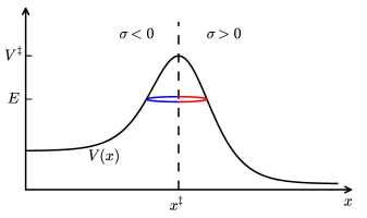
Figure 1: Schematic showing the instanton orbit modeling tunneling through a reaction barrier of height $V^{\ddagger}$. The orbit is made up of two trajectories that both start and end at the dividing surface $\sigma=x-x^{\ddagger}$ (dashed line) but bounce either on the left or right and contribute to $\Gamma^{-}$ or $\Gamma^{+}$ respectively.

Only trajectories starting and ending at the dividing surface contribute to Eq. (3). For a tunneling reaction, such as that depicted in Fig. 1, where the energy is lower than the barrier height, there will be two bouncing trajectories that encounter a turning point either on the $+$ or $-$ side of the dividing surface, where $\pm\sigma>0$. Those that bounce more than once can be ignored, as they have larger actions and therefore exponentially smaller contributions. The imaginary part of the Green’s function is then $\braket{\mathsf{x}^{\prime}}{\operatorname{Im}\hat{G}(E)}{\mathsf{x}^{\prime\prime}}\simeq\Gamma^{-}+\Gamma^{+}$, where the contribution from each trajectory is Richardson et al. (2015)

$$\Gamma^{\pm}\equiv\Gamma^{\pm}(\mathsf{x}^{\prime},\mathsf{x}^{\prime\prime},E)=-\frac{\pi\sqrt{\bar{D}^{\pm}}}{(2\pi\hbar)^{(f+1)/2}}\,\mathrm{e}^{-\bar{W}^{\pm}/\hbar}.$$ (6)

The abbreviated action is the following line integral along the respective classical trajectory:

$$\bar{W}^{\pm} \equiv\bar{W}^{\pm}(\mathsf{x}^{\prime},\mathsf{x}^{\prime\prime},E)=\int_{\mathsf{x}(q)=\mathsf{x}^{\prime\prime}}^{\mathsf{x}(q)=\mathsf{x}^{\prime}}\bar{p}(\mathsf{x})\,\mathrm{d}q,$$ (7)

$$\bar{p}(\mathsf{x}) =\sqrt{2m[V(\mathsf{x})-E]},$$ (8)

and the prefactors are

$$\bar{D}^{\pm} =(-1)^{f+1}\left|\begin{matrix}\frac{\partial^{2}{\bar{W}^{\pm}}}{\partial{\mathsf{x}^{\prime}}\partial{\mathsf{x}^{\prime\prime}}}&\frac{\partial^{2}{\bar{W}^{\pm}}}{\partial{\mathsf{x}^{\prime}}\partial{E}}\\ \frac{\partial^{2}{\bar{W}^{\pm}}}{\partial{E}\partial{\mathsf{x}^{\prime\prime}}}&\frac{\partial^{2}{\bar{W}^{\pm}}}{\partial{E}^{2}}\end{matrix}\right|=\frac{m^{2}}{\bar{p}(\mathsf{x}^{\prime})\bar{p}(\mathsf{x}^{\prime\prime})}A^{\pm},$$ (9)

$$A^{\pm} =\left|-\frac{\partial^{2}{\bar{W}^{\pm}}}{\partial{\mathsf{Q}^{\prime}}\partial{\mathsf{Q}^{\prime\prime}}}\right|,$$ (10)

where the coordinate system has been transformed from $\mathsf{x}$ to $(q,\mathsf{Q})$ Gutzwiller (1971), defined such that $q$ is parallel to the trajectory and equal to 0 at the dividing surface, and $\mathsf{Q}=(Q_{1},\dots,Q_{f-1})$ are the perpendicular modes .

The reaction probability, Eq. (3), requires not only matrix elements of the Green’s function but also the application of momentum operators on them. These operators can be written in the position basis as $\hat{p}_{j}=-\mathrm{i}\hbar\frac{\partial{}}{\partial{\hat{x}_{j}}}$, such that their effect is that of differentiation of the Green’s function Miller et al. (1983). However, because only the terms of the lowest order in $\hbar$ are required for the semiclassical approximation, the differentiation can be applied only to the exponential. The operator thus simply multiplies the Green’s function by $\pm\mathrm{i}\bar{p}(\mathsf{x}^{\prime})\frac{\partial{x_{j}^{\prime}}}{\partial{q^{\prime}}}$ (or the equivalent with double primes), which are the momentum components at the end points of the trajectory; they are imaginary and the sign depends on the direction traveled. Within the semiclassical approximation, therefore, the momentum operators act like classical variables.

Using the symmetry of $\Gamma^{\pm}(\mathsf{x}^{\prime},\mathsf{x}^{\prime\prime},E)=\Gamma^{\pm}(\mathsf{x}^{\prime\prime},\mathsf{x}^{\prime},E)$,

$$\rho(\mathsf{x}^{\prime},\mathsf{x}^{\prime\prime}) \simeq\mathrm{i}^{2}\Big{[}(\bar{p}_{\sigma}^{\prime}\Gamma^{-}-\bar{p}_{\sigma}^{\prime}\Gamma^{+})(\bar{p}_{\sigma}^{\prime\prime}\Gamma^{-}-\bar{p}_{\sigma}^{\prime\prime}\Gamma^{+})$$

$$\qquad+(-\bar{p}_{\sigma}^{\prime}\Gamma^{-}\bar{p}_{\sigma}^{\prime\prime}-\bar{p}_{\sigma}^{\prime}\Gamma^{+}\bar{p}_{\sigma}^{\prime\prime})(\Gamma^{-}+\Gamma^{+})\Big{]}$$ (11)

$$=4\bar{p}_{\sigma}^{\prime}\bar{p}_{\sigma}^{\prime\prime}\Gamma^{-}\Gamma^{+},$$ (12)

where $\bar{p}_{\sigma}^{\prime}=\left|\frac{\partial{\sigma}}{\partial{q^{\prime}}}\right|\bar{p}(\mathsf{x}^{\prime})$ is the magnitude of the momentum normal to the dividing surface at the end point $\mathsf{x}^{\prime}$; the definition with double primes is equivalent. All terms cancel except the cross term with trajectories that bounce once on the left and once on the right. Unlike for the QI method Miller et al. (2003), it was not necessary to introduce a second dividing surface to ensure this outcome . This is because spurious half-instantons, which cause Wigner’s TST to fail at low temperature Hele and Althorpe (2013), cannot form as trajectories contributing to $\operatorname{Im}\hat{G}(E)$ are required to bounce.

Therefore, using $\delta[\sigma(\mathsf{x})]=\delta(q)\left|\frac{\partial{\sigma}}{\partial{q}}\right|^{-1}$​, the semiclassical reaction probability is

$$P_{\text{SC}}(E)=(2\pi\hbar)^{1-f}\!\!\iiiint_{\text{SD}}\!\frac{\bar{p}(\mathsf{x}^{\prime})\bar{p}(\mathsf{x}^{\prime\prime})}{m^{2}}\sqrt{\bar{D}^{-}\bar{D}^{+}}\,\mathrm{e}^{-\bar{W}/\hbar}\\ \times\delta(q^{\prime})\delta(q^{\prime\prime})\,\mathrm{d}q^{\prime}\mathrm{d}q^{\prime\prime}\mathrm{d}\mathsf{Q}^{\prime}\mathrm{d}\mathsf{Q}^{\prime\prime},$$ (13)

where $\bar{W}=\bar{W}^{-}\!+\bar{W}^{+}$ is the total action along both trajectories. Performing the integrals over $\mathsf{Q}^{\prime}$ and $\mathsf{Q}^{\prime\prime}$ by the method of steepest descent (SD) gives

$$P_{\text{SC}}(E) =Z^{\ddagger}\,\mathrm{e}^{-\bar{W}/\hbar}$$ (14)

$$Z^{\ddagger} =\sqrt{A^{-}A^{+}}\begin{vmatrix}\frac{\partial^{2}{\bar{W}}}{\partial{\mathsf{Q}^{\prime}}\partial{\mathsf{Q}^{\prime}}}&\frac{\partial^{2}{\bar{W}}}{\partial{\mathsf{Q}^{\prime}}\partial{\mathsf{Q}^{\prime\prime}}}\\ \frac{\partial^{2}{\bar{W}}}{\partial{\mathsf{Q}^{\prime\prime}}\partial{\mathsf{Q}^{\prime}}}&\frac{\partial^{2}{\bar{W}}}{\partial{\mathsf{Q}^{\prime\prime}}\partial{\mathsf{Q}^{\prime\prime}}}\end{vmatrix}^{-{\frac{1}{2}}}\!\!.$$ (15)

All quantities are evaluated at the stationary point $\mathsf{x}^{\prime}=\mathsf{x}^{\prime\prime}=\mathsf{x}^{\ddagger}$ on the dividing surface where $\frac{\partial{\bar{W}}}{\partial{\mathsf{Q}^{\prime}}}=\frac{\partial{\bar{W}}}{\partial{\mathsf{Q}^{\prime\prime}}}=\mathsf{0}$. Here the trajectories join smoothly into each other to form a continuous periodic orbit, known as an instanton.

In the one-dimensional case, the formula reduces to $P_{\text{SC}}(E)=\mathrm{e}^{-\bar{W}/\hbar}$, which is the well-known WKB result Bell (1935). The appendix outlines a proof that $Z^{\ddagger}$ is a particular generalization of the partition function of the instanton such that $P_{\text{SC}}(E)$ is equivalent to an expression given by Miller in LABEL:Miller1975semiclassical. The final result is therefore independent of the choice of dividing surface and requires only that the instanton orbit intersects the surface at some point. The instanton could be thought of as defining a dividing region around the barrier Miller (1993).

Note that the short-time approximation inherent in the semiclassical Green’s functions is not necessarily valid when computing microcanonical rates as it cannot describe nuclear coherences leading, for instance, to discrete densities of states in a reactant well. The approximation is however asymptotically correct when energy is integrated over a smooth distribution such as the thermal distribution considered next.

The semiclassical thermal rate is found by evaluating the integral in Eq. (5) by steepest-descent Miller (1975) to give

$$k_{\text{SC}}Z_{\mathrm{r}} =(2\pi\hbar)^{-{\frac{1}{2}}}P_{\text{SC}}(E)\left(\frac{\mathrm{d}^{2}{\bar{W}}}{\mathrm{d}{E}^{2}}\right)^{-{\frac{1}{2}}}\mathrm{e}^{-\beta E},$$ (16)

where $E$ solves $\frac{\partial{\bar{W}}}{\partial{E}}=\beta\hbar$. As the imaginary time taken by each trajectory is $\tau^{\pm}=-\frac{\partial{\bar{W}^{\pm}}}{\partial{E}}$, the total time is $\beta\hbar$. The total derivatives are found using $q^{\prime}=q^{\prime\prime}=0$ and recognizing that $\mathsf{Q}^{\prime}$ and $\mathsf{Q}^{\prime\prime}$ are functions of $E$.

Assuming the barrier approximates the parabola $V(x)=-m\bar{\omega}^{2}x^{2}$ in one degree of freedom near its top, it cannot support periods less than $2\pi/\bar{\omega}$. The instanton approach is thus only defined for low temperatures when the periodic orbit exists. Extensions of the approach to treat higher temperatures, and involving terms with higher orders of $\hbar$, have been suggested Weiss (2008); Kryvohuz (2011); Zhang et al. (2014).

The result can be converted to the Lagrangian formulation using a Legendre transformation similar to that in LABEL:GoldenGreens. This is based on the full action,

$$\bar{S}^{\pm}\equiv\bar{S}^{\pm}(\mathsf{x}^{\prime},\mathsf{x}^{\prime\prime},\tau^{\pm})=\bar{W}^{\pm}(\mathsf{x}^{\prime},\mathsf{x}^{\prime\prime},E)+E\tau^{\pm},$$ (17)

where $E$ is defined such that the trajectories from $\mathsf{x}^{\prime\prime}$ to $\mathsf{x}^{\prime}$ are completed in imaginary time $\tau^{\pm}$. Using $\bar{S}=\bar{S}^{-}+\bar{S}^{+}$, and $\frac{\mathrm{d}^{2}{\bar{W}}}{\mathrm{d}{E}^{2}}=-\hbar\frac{\mathrm{d}{\beta}}{\mathrm{d}{E}}=-\hbar\big{(}\frac{\mathrm{d}{E}}{\mathrm{d}{\beta}}\big{)}^{-1}$​​, Eq. (16) becomes

$$k_{\text{SC}}Z_{\mathrm{r}} =(2\pi\hbar^{2})^{-\frac{1}{2}}\,Z^{\ddagger}\left(-\frac{\mathrm{d}{E}}{\mathrm{d}{\beta}}\right)^{{\frac{1}{2}}}\mathrm{e}^{-\bar{S}/\hbar},$$ (18)

which was also obtained by Miller Miller (1975), or equivalently

$$k_{\text{SC}}Z_{\mathrm{r}} =(2\pi\hbar)^{-{\frac{1}{2}}}\sqrt{\frac{\Sigma^{-}\Sigma^{+}}{-\Sigma}}\,\mathrm{e}^{-\bar{S}/\hbar},$$ (19)

where $\tau=\tau^{+}=\beta\hbar-\tau^{-}$ and, from LABEL:GoldenGreens,

$$\Sigma^{\pm}=\begin{vmatrix}\frac{\partial^{2}{\bar{S}^{\pm}}}{\partial{\mathsf{Q}^{\prime}}\partial{\mathsf{Q}^{\prime\prime}}}&\frac{\partial^{2}{\bar{S}^{\pm}}}{\partial{\mathsf{Q}^{\prime}}\partial{\tau^{\pm}}}\\ \frac{\partial^{2}{\bar{S}^{\pm}}}{\partial{\tau^{\pm}}\partial{\mathsf{Q}^{\prime\prime}}}&\frac{\partial^{2}{\bar{S}^{\pm}}}{\partial{\tau^{\pm}}\partial{\tau^{\pm}}}\end{vmatrix}=(-1)^{f-1}A^{\pm}\frac{\partial^{2}{\bar{S}^{\pm}}}{\partial{\tau^{\pm}}^{2}},$$

$$\Sigma=\frac{\mathrm{d}^{2}{\bar{S}}}{\mathrm{d}{\tau}^{2}}\begin{vmatrix}\frac{\partial^{2}{\bar{S}}}{\partial{\mathsf{Q}^{\prime}}\partial{\mathsf{Q}^{\prime}}}&\frac{\partial^{2}{\bar{S}}}{\partial{\mathsf{Q}^{\prime}}\partial{\mathsf{Q}^{\prime\prime}}}\\ \frac{\partial^{2}{\bar{S}}}{\partial{\mathsf{Q}^{\prime\prime}}\partial{\mathsf{Q}^{\prime}}}&\frac{\partial^{2}{\bar{S}}}{\partial{\mathsf{Q}^{\prime\prime}}\partial{\mathsf{Q}^{\prime\prime}}}\end{vmatrix}=\frac{\mathrm{d}^{2}{\bar{W}}}{\mathrm{d}{E}^{2}}\begin{vmatrix}\frac{\partial^{2}{\bar{W}}}{\partial{\mathsf{Q}^{\prime}}\partial{\mathsf{Q}^{\prime}}}&\frac{\partial^{2}{\bar{W}}}{\partial{\mathsf{Q}^{\prime}}\partial{\mathsf{Q}^{\prime\prime}}}\\ \frac{\partial^{2}{\bar{W}}}{\partial{\mathsf{Q}^{\prime\prime}}\partial{\mathsf{Q}^{\prime}}}&\frac{\partial^{2}{\bar{W}}}{\partial{\mathsf{Q}^{\prime\prime}}\partial{\mathsf{Q}^{\prime\prime}}}\end{vmatrix}.$$

Equation (19) can be evaluated numerically using the RPI algorithms to obtain the instanton and its action Richardson and Althorpe (2009) and derivatives Richardson (2015). This may lead to a better strategy for evaluating instanton rates in multidimensional complex systems than the standard RPI approach, Eq. (22), for which an $Nf\times Nf$ matrix must be diagonalized. Other approaches for locating the instanton orbit are also naturally suggested such as using the Hamilton-Jacobi formulation with end points constrained to bounce Richardson (2015) or modifications of the nudged-elastic-band method Einarsdóttir et al. (2012).

Following LABEL:Althorpe2011ImF, it can be shown that the semiclassical result Eq. (19) is equivalent to the RPI rate in the $N\rightarrow\infty$ limit Richardson and Althorpe (2009) and hence to the standard instanton rate theories Coleman (1977b); *Callan1977ImF; Affleck (1981); Benderskii et al. (1994). These are based on the $\operatorname{Im}F$ premise, $kZ_{\text{r}}\approx\frac{2}{\beta\hbar}\operatorname{Im}Z(\beta)$ Langer (1969); Weiss (2008) and the partition function can be evaluated in ring-polymer form as

$$Z(\beta) \equiv\mathrm{e}^{-\beta F}=\Lambda^{-Nf}\idotsint\mathrm{e}^{-\beta_{N}U_{N}(\mathbf{x})}\,\mathrm{d}\mathbf{x}.$$ (20)

Here, the integration is over $N$ ring-polymer beads $\mathbf{x}=\{\mathsf{x}_{1},\dots,\mathsf{x}_{N}\}$; $\beta_{N}=\beta/N$, $\Lambda=\sqrt{2\pi\beta_{N}\hbar^{2}/m}$ and the ring-polymer potential is

$$U_{N}(\mathbf{x})=\sum_{i=1}^{N}\frac{m}{2\beta_{N}^{2}\hbar^{2}}|\mathsf{x}_{i}-\mathsf{x}_{i+1}|^{2}+V(\mathsf{x}_{i}),$$ (21)

where the indices are cyclic such that $\mathsf{x}_{0}\equiv\mathsf{x}_{N}$. This is a discretization of the path-integral approach to quantum statistics Feynman and Hibbs (1965), and in the $N\rightarrow\infty$ limit, gives the partition function exactly.

The imaginary part of the partition function is, however, not well defined and it can only be obtained using analytic continuation. In practice, one takes a steepest-descent integral about the saddle point of $U_{N}(\mathbf{x})$ Richardson and Althorpe (2009); Althorpe (2011), but reverses the sign of the negative eigenvalue and multiplies the integral by a half Coleman (1977a); Kleinert (2006). There is also a zero-eigenvalue mode that is integrated out analytically. This procedure gives the RPI rate Richardson and Althorpe (2009),

$$k_{\text{RPI}}Z_{\text{r}} =\frac{\Lambda^{-1}}{\beta_{N}\hbar}\sqrt{\scriptsize{\sum\nolimits_{i=1}^{N}|\mathsf{x}_{i}-\mathsf{x}_{i-1}|^{2}}}\sideset{}{{}^{\prime}}{\prod}_{k}\left|\frac{1}{\beta_{N}\hbar\eta_{k}}\right|\mathrm{e}^{-\beta_{N}U_{N}}\!,$$ (22)

where $m\eta_{k}^{2}$ are the $Nf$ eigenvalues of the ring-polymer Hessian $\mathbf{\nabla}^{2}U_{N}$; the prime indicates that the mode for which $\eta_{k}=0$ is not included in the product.

Although Eq. (22) is the form employed in RPI calculations, equivalent expressions are found by taking the integrals in a different order Althorpe (2011). Steepest-descent integration of Eq. (20) over all beads but the two on the dividing surface gives

$$Z(\beta) \simeq 2\Lambda^{-2f}\iint\frac{1}{\sqrt{|\mathbf{J}^{-}||\mathbf{J}^{+}|}}\,\mathrm{e}^{-\bar{S}(\mathsf{x}^{\prime},\mathsf{x}^{\prime\prime})/\hbar}\,\mathrm{d}\mathsf{x}^{\prime}\mathrm{d}\mathsf{x}^{\prime\prime},$$ (23)

where the factor of 2 appears because of the degeneracy of the ring-polymer space, as the order of the beads along the orbit can be reversed. The square Hessian matrices $\mathbf{J}^{\pm}$ are defined as in LABEL:GoldenRPI from second-derivatives of $U_{N}(\mathbf{x})$ with respect to the beads on the $\pm\sigma>0$ side of the dividing surface. A further coordinate transformation, $\mathrm{d}\mathsf{x}^{\prime}=\mathrm{d}q^{\prime}\mathrm{d}\mathsf{Q}^{\prime}=\dot{q}^{\prime}\mathrm{d}\tau^{\prime}\mathrm{d}\mathsf{Q}^{\prime}$, describes the position along the trajectory using imaginary time. The instanton orbit folds back on itself so $\tau^{\prime}$ has a range of ${\frac{1}{2}}\beta\hbar$ and $\dot{q}^{\prime}=\left|\frac{\mathrm{d}{q^{\prime}}}{\mathrm{d}{\tau^{\prime}}}\right|$, which could be estimated using $|\mathsf{x}_{i+1}-\mathsf{x}_{i}|/\beta_{N}\hbar$ and the appropriate index $i$. The equivalent holds for double primes. Due to the cyclic permutational symmetry around the ring polymer Richardson and Althorpe (2009), the integral over one time variable is simple giving

$$Z(\beta) \simeq 2\Lambda^{-2f}\iiint\frac{{\frac{1}{2}}\beta\hbar\dot{q}^{\prime}\dot{q}^{\prime\prime}}{\sqrt{|\mathbf{J}^{-}||\mathbf{J}^{+}|}}\,\mathrm{e}^{-\bar{S}/\hbar}\,\mathrm{d}\tau\mathrm{d}\mathsf{Q}^{\prime}\mathrm{d}\mathsf{Q}^{\prime\prime},$$ (24)

whereas the second over the remaining $\tau$ is completed, according to the usual $\operatorname{Im}F$ procedure, using analytic continuation of steepest-descent over an imaginary mode and multiplying by a factor of half:

$$\operatorname{Im}Z(\beta) \simeq\frac{\sqrt{2\pi\hbar}}{\Lambda^{2f}}\!\iint\!\frac{{\frac{1}{2}}\beta\hbar\dot{q}^{\prime}\dot{q}^{\prime\prime}}{\sqrt{|\mathbf{J}^{-}||\mathbf{J}^{+}|}}\left|\frac{\mathrm{d}^{2}{\bar{S}}}{\mathrm{d}{\tau}^{2}}\right|^{-{\frac{1}{2}}}\!\mathrm{e}^{-\bar{S}/\hbar}\,\mathrm{d}\mathsf{Q}^{\prime}\mathrm{d}\mathsf{Q}^{\prime\prime}.$$

The remaining integrals over the perpendicular directions are performed using steepest-descent to give

$$k_{\text{RPI}}Z_{\text{r}} =(2\pi\hbar)^{-{\frac{1}{2}}}\left(\frac{m}{\beta_{N}\hbar}\right)^{f}\frac{\dot{q}^{2}|\Sigma|^{-1/2}}{\sqrt{|\mathbf{J}^{-}||\mathbf{J}^{+}|}}\,\mathrm{e}^{-\bar{S}/\hbar},$$ (25)

where at the stationary point $\dot{q}^{\prime}=\dot{q}^{\prime\prime}=\dot{q}$. In the $N\rightarrow\infty$ limit, this formulation is equivalent to all $\operatorname{Im}F$ instanton rates Coleman (1977b); *Callan1977ImF; Affleck (1981); Benderskii et al. (1994); Richardson and Althorpe (2009); Andersson et al. (2009); *Andersson2011HCO; *Jonsson2011surface; Pérez de Tudela et al. (2014); Goumans and Kästner (2010); *Goumans2011Hmethanol; *Meisner2011isotope; *Rommel2011locating; *Rommel2011grids; *Rommel2012enzyme; *Kaestner2013carbenes; *Kaestner2014review including Eq. (22).

It is now a simple matter to show that Eq. (25) is equivalent to the first-principles rate derived above from the semiclassical Green’s functions, i.e. $k_{\text{SC}}=\lim_{N\rightarrow\infty}k_{\text{RPI}}$. From Eq. (9), and using a number of relations stated in Refs. Richardson et al. (2015); Richardson (2015), the necessary equations are

$$(-1)^{f+1}\Sigma^{\pm}/\dot{q}^{2} =\left|-\frac{\partial^{2}{\bar{S}^{\pm}}}{\partial{\mathsf{x}^{\prime}}\partial{\mathsf{x}^{\prime\prime}}}\right|=\left(\frac{m}{\beta_{N}\hbar}\right)^{f}|\mathbf{J}^{\pm}|^{-1}.$$ (26)

In summary, the instanton method for computing the rate of tunneling through a barrier on a Born-Oppenheimer potential-energy surface has been rederived from a semiclassical limit of scattering theory Miller et al. (1983). The final form is exactly equivalent to the usual expression given by the $\operatorname{Im}F$ premise, although the derivation is more rigorous. The semiclassical instanton appears from the reaction probability at a given energy before temperature has been introduced. This is in contrast with other path-integral rate theories based on the Boltzmann operator Gillan (1987); Voth et al. (1989); Makarov and Topaler (1995); Cao and Voth (1996); Mills et al. (1997); Habershon et al. (2013); Hele and Althorpe (2013). Real-time dynamical information does not contribute, as is appropriate for a complex dissipative system where nuclear coherence is washed out. However, unlike TST or QI methods Gillan (1987); Voth et al. (1989); Makarov and Topaler (1995); Cao and Voth (1996); Mills et al. (1997); Hele and Althorpe (2013); Miller et al. (2003); Vaníček et al. (2005), the instanton rate remains independent of the dividing surface so long as the instanton orbit intersects it. In light of this new derivation, applications of instanton methods can be better understood and the development of new RPMD and QI approaches advanced. Generalizations of the new derivation provide a new route to solving novel problems such as nonadiabatic reaction rates Richardson et al. (2015).

The author would like to thank Stuart C. Althorpe and William H. Miller for helpful comments on the manuscript. This work was supported by the Alexander von Humboldt Foundation and a European Union COFUND/Durham Junior Research Fellowship.

Appendix A Appendix

In the main text it was claimed that the instanton partition function $Z^{\ddagger}$ is equivalent to that given by Miller Miller (1975), which is expressed in terms of the stability parameters, $u_{j}(E)$, of the instanton orbit Whittaker (1917); Pars (1965); Gutzwiller (1971); Miller (1975). This can be shown indirectly using the results from the main text that the semiclassical rate, $k_{\text{SC}}$, is equivalent to the $\operatorname{Im}F$ form, $k_{\text{RPI}}$, and the proof in LABEL:Althorpe2011ImF that $k_{\text{RPI}}$ is equivalent to Miller’s rate Miller (1975). However, it is also possible to provide a more direct proof as outlined in this appendix.

The instanton was derived as the conjunction of two imaginary-time trajectories. In order to make the connection with stability parameters, it will be necessary to make a transformation of the defining variables to describe the instanton as a single periodic orbit. The following derivation is similar to that followed in Section 4.4 of LABEL:Kleinert. The analysis applies equally to real-time and imaginary-time trajectories and the notation of a bar over the action is dropped here.

Consider first a classical trajectory with fixed energy, $E$, traveling from $(q_{a},\mathsf{Q}_{a})$ to $(q_{b},\mathsf{Q}_{b})$ with abbreviated action $W^{-}\equiv W^{-}(\mathsf{Q}_{a},\mathsf{Q}_{b})$ and then continuing from $(q_{b},\mathsf{Q}_{b})$ to $(q_{c},\mathsf{Q}_{c})$ with abbreviated action $W^{+}\equiv W^{+}(\mathsf{Q}_{b},\mathsf{Q}_{c})$. The coordinate system is chosen such that the $q$ coordinate is parallel to the trajectory and $\mathsf{Q}$ perpendicular and $q_{a}$, $q_{b}$ and $q_{c}$ are fixed. In order that the two parts of the trajectory join correctly, $\mathsf{Q}_{b}=\mathsf{Q}_{b}(\mathsf{Q}_{a},\mathsf{Q}_{c})$ must be defined such that

$$\frac{\partial{W^{-}}}{\partial{\mathsf{Q}_{b}}}+\frac{\partial{W^{+}}}{\partial{\mathsf{Q}_{b}}}=\mathsf{0}.$$ (27)

Thus the two trajectories combine to give one classical trajectory from $(q_{a},\mathsf{Q}_{a})$ to $(q_{c},\mathsf{Q}_{c})$ with abbreviated action

$$\tilde{W}\equiv\tilde{W}(\mathsf{Q}_{a},\mathsf{Q}_{c})=W^{-}(\mathsf{Q}_{a},\mathsf{Q}_{b})+W^{+}(\mathsf{Q}_{b},\mathsf{Q}_{c}).$$ (28)

This situation is summarized in Fig. 2.

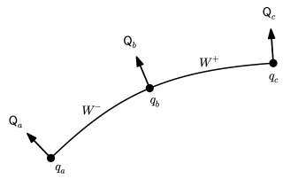
Figure 2: Schematic showing a classical trajectory traveling between points $(q_{a},\mathsf{Q}_{a})$ and $(q_{c},\mathsf{Q}_{c})$ and which passes through $(q_{b},\mathsf{Q}_{b})$. The coordinates are parallel ($q$) and perpendicular ($\mathsf{Q}$) to the trajectory. The abbreviated action $W^{\pm}$ along each segment is marked.

Partial differentiation of Eq. (28) using the chain rule gives

$$\frac{\partial^{2}{\tilde{W}}}{\partial{\mathsf{Q}_{a}}\partial{\mathsf{Q}_{c}}}=\frac{\partial^{2}{W^{-}}}{\partial{\mathsf{Q}_{a}}\partial{\mathsf{Q}_{b}}}\frac{\partial{\mathsf{Q}_{b}}}{\partial{\mathsf{Q}_{c}}}=\frac{\partial^{2}{W^{+}}}{\partial{\mathsf{Q}_{c}}\partial{\mathsf{Q}_{b}}}\frac{\partial{\mathsf{Q}_{b}}}{\partial{\mathsf{Q}_{a}}}$$ (29)

and of Eq. (27) gives

$$-\left.\frac{\partial^{2}{W^{+}}}{\partial{\mathsf{Q}_{b}}\partial{\mathsf{Q}_{b}}}\right|_{\mathsf{Q}_{c}} =\left.\frac{\partial^{2}{W^{-}}}{\partial{\mathsf{Q}_{b}}\partial{\mathsf{Q}_{b}}}\right|_{\mathsf{Q}_{c}}=\frac{\partial^{2}{W^{-}}}{\partial{\mathsf{Q}_{b}}\partial{\mathsf{Q}_{a}}}\frac{\partial{\mathsf{Q}_{a}}}{\partial{\mathsf{Q}_{b}}}+\left.\frac{\partial^{2}{W^{-}}}{\partial{\mathsf{Q}_{b}}\partial{\mathsf{Q}_{b}}}\right|_{\mathsf{Q}_{a}},$$ (30a)

$$-\left.\frac{\partial^{2}{W^{-}}}{\partial{\mathsf{Q}_{b}}\partial{\mathsf{Q}_{b}}}\right|_{\mathsf{Q}_{a}} =\left.\frac{\partial^{2}{W^{+}}}{\partial{\mathsf{Q}_{b}}\partial{\mathsf{Q}_{b}}}\right|_{\mathsf{Q}_{a}}=\frac{\partial^{2}{W^{+}}}{\partial{\mathsf{Q}_{b}}\partial{\mathsf{Q}_{c}}}\frac{\partial{\mathsf{Q}_{c}}}{\partial{\mathsf{Q}_{b}}}+\left.\frac{\partial^{2}{W^{+}}}{\partial{\mathsf{Q}_{b}}\partial{\mathsf{Q}_{b}}}\right|_{\mathsf{Q}_{c}}.$$ (30b)

In combination, they give

$$\frac{\partial^{2}{\tilde{W}}}{\partial{\mathsf{Q}_{a}}\partial{\mathsf{Q}_{a}}} =\frac{\partial^{2}{W^{-}}}{\partial{\mathsf{Q}_{a}}\partial{\mathsf{Q}_{a}}}-\frac{\partial^{2}{W^{-}}}{\partial{\mathsf{Q}_{a}}\partial{\mathsf{Q}_{b}}}\left(\frac{\partial^{2}{W^{-}}}{\partial{\mathsf{Q}_{b}}\partial{\mathsf{Q}_{b}}}+\frac{\partial^{2}{W^{+}}}{\partial{\mathsf{Q}_{b}}\partial{\mathsf{Q}_{b}}}\right)^{-1}\frac{\partial^{2}{W^{-}}}{\partial{\mathsf{Q}_{b}}\partial{\mathsf{Q}_{a}}}$$ (31a)

$$\frac{\partial^{2}{\tilde{W}}}{\partial{\mathsf{Q}_{a}}\partial{\mathsf{Q}_{c}}} =-\frac{\partial^{2}{W^{-}}}{\partial{\mathsf{Q}_{a}}\partial{\mathsf{Q}_{b}}}\left(\frac{\partial^{2}{W^{-}}}{\partial{\mathsf{Q}_{b}}\partial{\mathsf{Q}_{b}}}+\frac{\partial^{2}{W^{+}}}{\partial{\mathsf{Q}_{b}}\partial{\mathsf{Q}_{b}}}\right)^{-1}\frac{\partial^{2}{W^{+}}}{\partial{\mathsf{Q}_{b}}\partial{\mathsf{Q}_{c}}}$$ (31b)

$$\frac{\partial^{2}{\tilde{W}}}{\partial{\mathsf{Q}_{c}}\partial{\mathsf{Q}_{a}}} =-\frac{\partial^{2}{W^{+}}}{\partial{\mathsf{Q}_{c}}\partial{\mathsf{Q}_{b}}}\left(\frac{\partial^{2}{W^{-}}}{\partial{\mathsf{Q}_{b}}\partial{\mathsf{Q}_{b}}}+\frac{\partial^{2}{W^{+}}}{\partial{\mathsf{Q}_{b}}\partial{\mathsf{Q}_{b}}}\right)^{-1}\frac{\partial^{2}{W^{-}}}{\partial{\mathsf{Q}_{b}}\partial{\mathsf{Q}_{a}}}$$ (31c)

$$\frac{\partial^{2}{\tilde{W}}}{\partial{\mathsf{Q}_{c}}\partial{\mathsf{Q}_{c}}} =\frac{\partial^{2}{W^{+}}}{\partial{\mathsf{Q}_{c}}\partial{\mathsf{Q}_{c}}}-\frac{\partial^{2}{W^{+}}}{\partial{\mathsf{Q}_{c}}\partial{\mathsf{Q}_{b}}}\left(\frac{\partial^{2}{W^{-}}}{\partial{\mathsf{Q}_{b}}\partial{\mathsf{Q}_{b}}}+\frac{\partial^{2}{W^{+}}}{\partial{\mathsf{Q}_{b}}\partial{\mathsf{Q}_{b}}}\right)^{-1}\frac{\partial^{2}{W^{+}}}{\partial{\mathsf{Q}_{b}}\partial{\mathsf{Q}_{c}}},$$ (31d)

and thus

$$\frac{\partial^{2}{\tilde{W}}}{\partial{\mathsf{Q}_{a}}\partial{\mathsf{Q}_{a}}}+\frac{\partial^{2}{\tilde{W}}}{\partial{\mathsf{Q}_{a}}\partial{\mathsf{Q}_{c}}}+\frac{\partial^{2}{\tilde{W}}}{\partial{\mathsf{Q}_{c}}\partial{\mathsf{Q}_{a}}}+\frac{\partial^{2}{\tilde{W}}}{\partial{\mathsf{Q}_{c}}\partial{\mathsf{Q}_{c}}}\\ =\frac{\partial^{2}{W^{-}}}{\partial{\mathsf{Q}_{a}}\partial{\mathsf{Q}_{a}}}+\frac{\partial^{2}{W^{+}}}{\partial{\mathsf{Q}_{c}}\partial{\mathsf{Q}_{c}}}-\left(\frac{\partial^{2}{W^{-}}}{\partial{\mathsf{Q}_{a}}\partial{\mathsf{Q}_{b}}}+\frac{\partial^{2}{W^{+}}}{\partial{\mathsf{Q}_{c}}\partial{\mathsf{Q}_{b}}}\right)\left(\frac{\partial^{2}{W^{-}}}{\partial{\mathsf{Q}_{b}}\partial{\mathsf{Q}_{b}}}+\frac{\partial^{2}{W^{+}}}{\partial{\mathsf{Q}_{b}}\partial{\mathsf{Q}_{b}}}\right)^{-1}\left(\frac{\partial^{2}{W^{-}}}{\partial{\mathsf{Q}_{b}}\partial{\mathsf{Q}_{a}}}+\frac{\partial^{2}{W^{+}}}{\partial{\mathsf{Q}_{b}}\partial{\mathsf{Q}_{c}}}\right).$$ (32)

These are the transformation equations for the general case of a trajectory split into two components.

The periodic instanton orbit is a special case of the trajectory considered above as its end points meet. Using the notation from the main text, it is defined with abbreviated action

$$W(\mathsf{Q}^{\prime},\mathsf{Q}^{\prime\prime})=W^{-}(\mathsf{Q}^{\prime},\mathsf{Q}^{\prime\prime})+W^{+}(\mathsf{Q}^{\prime\prime},\mathsf{Q}^{\prime}),$$ (33)

where $q_{a}=q_{b}=q_{c}=0$, $\mathsf{Q}_{a}=\mathsf{Q}_{c}=\mathsf{Q}^{\prime}$ and $\mathsf{Q}_{b}=\mathsf{Q}^{\prime\prime}$.

The instanton partition function, from Eq. (15), is therefore

$$Z^{\ddagger} =\sqrt{A^{-}A^{+}}\begin{vmatrix}\frac{\partial^{2}{W}}{\partial{\mathsf{Q}^{\prime}}\partial{\mathsf{Q}^{\prime}}}&\frac{\partial^{2}{W}}{\partial{\mathsf{Q}^{\prime}}\partial{\mathsf{Q}^{\prime\prime}}}\\ \frac{\partial^{2}{W}}{\partial{\mathsf{Q}^{\prime\prime}}\partial{\mathsf{Q}^{\prime}}}&\frac{\partial^{2}{W}}{\partial{\mathsf{Q}^{\prime\prime}}\partial{\mathsf{Q}^{\prime\prime}}}\end{vmatrix}^{-{\frac{1}{2}}}$$ (34)

$$=\sqrt{\frac{\Psi}{\Phi}}$$ (35)

where

$$\Phi =\left|\frac{\partial^{2}{W}}{\partial{\mathsf{Q}^{\prime}}\partial{\mathsf{Q}^{\prime}}}-\frac{\partial^{2}{W}}{\partial{\mathsf{Q}^{\prime}}\partial{\mathsf{Q}^{\prime\prime}}}\left(\frac{\partial^{2}{W}}{\partial{\mathsf{Q}^{\prime\prime}}\partial{\mathsf{Q}^{\prime\prime}}}\right)\frac{\partial^{2}{W}}{\partial{\mathsf{Q}^{\prime\prime}}\partial{\mathsf{Q}^{\prime}}}\right|$$ (36)

$$=\left|\frac{\partial^{2}{\tilde{W}}}{\partial{\mathsf{Q}_{a}}\partial{\mathsf{Q}_{a}}}+2\frac{\partial^{2}{\tilde{W}}}{\partial{\mathsf{Q}_{a}}\partial{\mathsf{Q}_{c}}}+\frac{\partial^{2}{\tilde{W}}}{\partial{\mathsf{Q}_{c}}\partial{\mathsf{Q}_{c}}}\right|$$ (37)

and

$$\Psi =A^{-}\left|\frac{\partial^{2}{W}}{\partial{\mathsf{Q}^{\prime\prime}}\partial{\mathsf{Q}^{\prime\prime}}}\right|^{-1}A^{+}$$ (38)

$$=\left|\frac{\partial^{2}{W^{-}}}{\partial{\mathsf{Q}_{a}}\partial{\mathsf{Q}_{b}}}\left(\frac{\partial^{2}{W^{-}}}{\partial{\mathsf{Q}_{b}}\partial{\mathsf{Q}_{b}}}+\frac{\partial^{2}{W^{+}}}{\partial{\mathsf{Q}_{b}}\partial{\mathsf{Q}_{b}}}\right)^{-1}\frac{\partial^{2}{W^{+}}}{\partial{\mathsf{Q}_{b}}\partial{\mathsf{Q}_{c}}}\right|$$ (39)

$$=\left|-\frac{\partial^{2}{\tilde{W}}}{\partial{\mathsf{Q}_{a}}\partial{\mathsf{Q}_{c}}}\right|$$ (40)

Section 4 of LABEL:Gutzwiller1971orbits shows that the ratio of these determinants gives

$$Z^{\ddagger} =\prod_{j=1}^{f-1}\frac{1}{2\sinh[u_{j}(E)/2]}$$ (41)

where $u_{j}(E)$ are the non-zero stability parameters of the periodic orbit. It is known that the stability parameters do not depend on the position $q_{a}=q_{c}$ around the orbit Gutzwiller (1971) and thus it is proved that, as stated in the main text, the semiclassical reaction probability is independent of the form of the dividing surface. The same stability parameters also appear in Miller’s instanton theory Miller (1975) which is therefore equal to the semiclassical rate derived in the main text.