Global existence for a degenerate haptotaxis model of cancer invasion

Abstract

We propose and study a strongly coupled PDE-ODE system with tissue-dependent degenerate diffusion and haptotaxis that can serve as a model prototype for cancer cell invasion through the extracellular matrix. We prove the global existence of weak solutions and illustrate the model behaviour by numerical simulations for a two-dimensional setting.

Keywords: cancer cell invasion; degenerate diffusion; global existence; haptotaxis; parabolic system; weak solution.
MSC 2010: 35B45, 35D30, 35K20, 35K51, 35K57, 35K59, 35K65, 35Q92, 92C17.

1 Introduction

Cancer cell migration is an essential step in the development and expansion of a tumor and its metastases. Thereby, diffusion and taxis are two of the main vehicles of cancer cell motility. The term ’taxis’ characterizes the movement in the direction of the gradient of some signal available in the peritumoral region and –depending on the nature of the stimulus– refers to chemotaxis (directed cell motion in response to a chemical concentration gradient), haptotaxis (motion follows the gradient of the density of tissue fibers), pH-taxis (direction of motion dictated by a pH gradient) etc. While chemotaxis gradients may lack in the solution, haptotaxis seems to be indispensable, as the cells need to adhere to the ECM in order to support their motion [1], but also for information exchange with their surroundings, the latter being closely related to survival and proliferation [20, 30], see also [29] for a comprehensive review. For these reasons we focus here on diffusion and haptotaxis. The latter is triggered by an unsoluble stimulus: the fibers of the extracellular matrix (ECM) and their density.
Biological experiments suggest that:

• enhanced interactions with the surrounding tissue favor cell motility (in particular, diffusivity) [13];

• in those areas where the cells and the ECM are tightly packed, the diffusivity and the advective effects of haptotaxis (and hence also the invasion into the tissue) are limited [23];

• no cell migration (in particular no diffusivity) occurs in regions where the tissue is absent (see above);

• cells propagate through the ECM with a finite speed.

As mentioned already, haptotaxis is connected to directioning the motion along the gradient of an immovable stimulus (density of tissue fibers). Therefore, the evolution of the latter is characterized by way of an ODE. Since it contains no spatial diffusion, this ODE corresponds to an everywhere degenerate reaction-diffusion PDE and has no regularising effect. When strongly coupled to a PDE for the cell density via a haptotactic transport term, this causes a considerable difficulty for the analysis.

Previous models for cell migration involving haptotaxis and operating on the macroscopic scale of population densities have been proposed e.g., in [4, 8, 7] upon relying on equilibrium of fluxes (diffusion and haptotaxis, possibly with some other kinds of taxis as well). The mathematical analysis of this model class was most often performed in the case with linear diffusion for the tumor cell density, see e.g., [24, 35, 37] and only recently approached for settings allowing for nonlinear diffusion [36, 38]. Still, in the pure macroscopic framework, nonlocal models including cell-cell and cell-tissue interactions within a sensing radius by way of integral terms have been proposed and simulated [5, 14, 27, 31]. The mathematical analysis (well posedness of classical solutions) of a couple of models in that class, however in some simplified settings –yet with linear diffusion– has been done in [9, 34].

Multiscale models for cancer cell migration involving haptotaxis and coupling subcellular dynamics (microlevel) with population dynamics (macroscale) have been recently proposed and investigated with respect to well posedness in [25, 33], also considering nonlinear diffusion for the tumor cell density. A further micro-macro model for acid-mediated tumor invasion through tissue and allowing for gap formation at the tumor interface was proposed in [15] and its global well-posedness shown; the model also accounts for stochastic effects, nonlinear diffusion, and repellent taxis. Yet another multiscale model class for tumor invasion with (chemo- and) haptotaxis is that considered and analyzed in [18, 22]. Those models couple subcellular dynamics (ODEs) with mesoscopic kinetic transport equations describing individual cell behavior and the evolution of tissue fiber density, and with the macrolevel dynamics of a chemoattractant concentration. Those models are able to account for nonlinear diffusion, meaning that the diffusion coefficient in the equation for cell density is allowed to depend on the solution itself.

In the quasilinear system handled in [33] the diffusion coefficient of the cell density depends, moreover, upon the local interaction between the tumor cells and the ECM fibers. However, that coefficient was still assumed to be nondegenerate (at least as long as the solutions remain bounded), and thus the model did not capture the features (iii) and (iv) listed above. In order to account for all properties (i)-(iv) we develop in this paper a degenerate-diffusion system, thereby keeping only two components: the density of the tumor cells and the density of the tissue fibers, hence studying a model with diffusion and haptotaxis only. As we focus here on the degeneracy issue in the framework of a haptotaxis model we ignore the multiscality and stay on the population level. For this new prototype model we prove the global existence of weak solutions. The uniqueness and boundedness of solutions remain open.

This paper is organised as follows: In Section 2 we set up the mathematical model, followed by fixing some notations in Section 3 and by the statement of the problem and the main result in Section 4. The subsequent Sections 5, 6, and 7 are dedicated to the proof of this result, by constructing sequences of nondegenerate approximations to the original problems, proving some apriori estimates for these approximations, and passing to the limits in the approximations, respectively. In Section 8, we illustrate the possible model behaviour by performing numerical simulations in the two-dimensional case and compare the results with those reproduced for a previous model with nondegenerate diffusion of the tumor cells. Finally, we provide in Section 9 a short discussion of the obtained results and set them in context with respect to other models with degenerate diffusion. The paper includes an Appendix with two auxiliary results (Lemmata A.1 and  A.2) dealing with weak and almost everywhere convergence and being of independent interest.

2 The model

In this section we introduce an ODE-PDE system for two variables: the cancer cells density $c$ and the density $v$ of ECM tissue fibers, both depending on time and position on a smooth bounded domain $\Omega\subset\mathbb{R}^{N}$. Our system, a variant of the one introduced in [33], has the following form:

$$\partial_{t}c=\nabla\cdot\left(\frac{\kappa_{c}vc}{1+vc}\nabla c-\frac{\kappa_{v}c}{(1+v)^{2}}\nabla v\right)+\mu_{c}c(1-c-\eta v) \text{ in }\mathbb{R}^{+}\times\Omega,$$ (2.1a)

$$\partial_{t}v=\mu_{v}v(1-v)-\lambda vc \text{ in }\mathbb{R}^{+}\times\Omega,$$ (2.1b)

$$\frac{\kappa_{c}vc}{1+vc}\partial_{\nu}c-\frac{\kappa_{v}c}{(1+v)^{2}}\partial_{\nu}v=0 \text{ in }\mathbb{R}^{+}\times\partial\Omega,$$ (2.1c)

$$c(0)=c_{0},\ v(0)=v_{0} \text{ in }\Omega,$$ (2.1d)

where $\kappa_{c},\kappa_{v},\mu_{c},\eta,\mu_{v},\lambda$ are some positive constants. System (2.1) consists of a degenerate parabolic PDE which describes the evolution of the tumor cell density and an ODE for the evolution of the tissue density, supplemented by the initial and the ’no-flux’ boundary conditions. The latter is realistic, since the cancer cells do not leave the tissue hosting the original tumor.
Equation (2.1a) for the tumor cell density includes two nonlinear spatial movement effects: degenerate diffusion and haptotaxis transport.
The nonlinear diffusion coefficient in (2.1a) is taken to be of the form

$$D_{c}(v,c):=\frac{\kappa_{c}vc}{1+vc},$$

where the positive constant $\kappa_{c}$ accounts for the adhesivity between the tumor cells and the fiber. Notice that the source of degeneracy is twofold: the diffusion coefficient can become zero when $c=0$, but also when $v=0$. Our choice of the diffusion coefficient is less restrictive than previous settings which involve some powers of the solution, chosen in such a way as to render the mathematical analysis more amenable. Instead, the choice of our degenerate diffusion coefficient is motivated by the biological phenomenon under consideration, more precisely by the four properties of the cell spreading which we proposed in Section 1. Indeed, let us consider the product $cv$ as a measure of interaction between the cells and the tissue. Then, we have that:

• $D_{c}$ is monotonically increasing in $vc$;

• $\underset{vc\rightarrow\infty}{\lim}D_{c}(v,c)=\kappa_{c}<\infty$;

• $D_{c}(0,c)=0$ for all $c\in\mathbb{R}_{0}^{+}$;

• $D_{c}(v,c)\underset{c\rightarrow 0}{\approx}\kappa_{c}vc$ for all $v\in\mathbb{R}_{0}^{+}$.

The first three properties above clearly correspond to (i)-(iii) from the introduction. As for the last property, the porous-medium type degeneracy with respect to variable $c$ is known to ensure a finite speed of propagation, which provides the condition (iv) in Section 1. It seems that [17] was the first paper involving a diffusion coefficient of the form $\kappa_{c}vc$, there in the context of bacterial biofilm dispersal.
The signal-dependent haptotactic sensitivity function

$$\chi(v):=\frac{\kappa_{v}}{(1+v)^{2}}$$ (2.2)

is obtained upon accounting for receptor binding to ECM fibers. Here, however, we avoid including specific subcellular dynamics and simplify the setting by looking directly at cell-tissue interactions instead of receptor-ligand bindings. Indeed, consider the ’mass action kinetics’

$$c+v\underset{k^{-}}{\stackrel{{\scriptstyle k^{+}}}{{\rightleftharpoons}}}[cv],$$

leading to the ODE system

$$\partial_{t}c =k^{-}[cv]-k^{+}cv$$

$$\partial_{t}v =k^{-}[cv]-k^{+}cv$$

$$\partial_{t}[cv] =k^{+}cv-k^{-}[cv].$$

As the binding kinetics is very fast, we may assume that the corresponding steady-state is quickly achieved, hence from the last equation above we obtain

$$[cv]=\frac{k^{+}}{k^{-}}cv.$$ (2.3)

Furthermore, we assume the total amount of cells is conserved during this short time span, hence

$$c+[cv]=\text{const}.$$

This leads to $c=\text{const}-[cv]$ and plugging into (2.3) and using the notation $\kappa:=\frac{k^{+}}{k^{-}}$ we get

$$[cv]=\frac{\text{const}\cdot v}{\kappa+v}.$$

The haptotaxis equation is obtained by equilibrium of fluxes, but it can also be deduced from a master equation written with the aid of the corresponding probabilities (rates) $T_{i}^{\pm}$ of transition from a position $i$ into the adjacent one $i-1$ or $i+1$, respectively. With the gradient-based choice (see e.g., [26])

$$T_{i}^{\pm}:=\alpha+\beta(\tau(v_{i})-\tau(v_{i\pm 1})),\quad\alpha>0,\ \beta\geq 0,$$

where $\tau$ is a known differentiable function, we get for the haptotaxis coefficient the form $\chi(v)c$, with $\chi(v)=2\beta\tau^{\prime}(v)$. As $\tau(v)$ characterizes the (chemical) mechanism of measuring tissue densities, we can interpret $\tau(v)$ as giving the amount of cell surface receptors bound to the tissue fibers, or –even further simplified, to avoid introducing the subcellular scale explicitly– the amount of cells bound to ECM fibers, hence $\tau(v)=[cv]=\frac{\text{const}\cdot v}{\kappa+v}$. This leads to

$$\chi(v)=2\beta\frac{\text{const}\cdot\kappa}{(\kappa+v)^{2}},$$

which is of the form (2.2) announced above.
The equation (2.1b) for the tissue density $v$ is an ODE. It contains no spatial movement effects since the ECM fibers do not move on their own. They can be deformed, at most, but we ignore here such deformations.

3 Basic notation and functional spaces

Partial derivatives, in both classical and distributional sense, with respect to variables $t$ and $x_{i}$, will be denoted respectively by $\partial_{t}$ and $\partial_{x_{i}}$. Further, $\nabla$, $\nabla\cdot$ and $\Delta$ stand for the spatial gradient, divergence and Laplace operators, respectively. $\partial_{\nu}$ is the derivative with respect to the outward unit normal of $\partial\Omega$.

We assume the reader to be familiar with the standard $L^{p}$, Sobolev, and Hölder spaces and their usual properties, as well as with the more general $L^{p}$ spaces of functions with values in general Banach spaces and with anisotropic Sobolev spaces. In particular, we need the space

$$W^{-1,1}(\Omega):=\left\{u\in D^{\prime}(\Omega)|\ u=u_{0}+\sum_{k=1}^{N}\partial_{x_{i}}u_{i}\text{ for some }u_{i}\in L^{1}\left(\Omega\right),\ i=1,\dots,N\right\}.$$

For $p\in[1,\infty]\backslash\left\{2\right\}$, we write $||\cdot||_{p}$ in place of the $||\cdot||_{L^{p}\left(\Omega\right)}$-norm. Throughout the paper, $||\cdot||$ stands for the $||\cdot||_{L^{2}\left(\Omega\right)}$-norm and $(u,v)$ for $\int_{\Omega}u(x)v(x)\,dx$, while $\left<\cdot,\cdot\right>$ is reserved for the duality pairing between $W^{1,\infty}(\Omega)$ and its dual $(W^{1,\infty}(\Omega))^{\prime}$.

We denote the Lebesgue measure of a set $A$ by $|A|$ and by $\operatorname{int}A$ its interior.

Finally, we make the following useful convention: For all indices $i$, the quantity $C_{i}$ denotes a non-negative constant or, alternatively, a non-negative function, which is non-decreasing in each of its arguments.

4 Problem setting and main result

In this section we propose a definition of weak solutions to system (2.1) and state our main result under the following assumptions:

Assumptions 4.1 (Initial data).

1. $c_{0}\geq 0,\ c_{0}\nequiv 0,\ c_{0}\ln c_{0}\in L^{1}\left(\Omega\right)$;

2. $0\leq v_{0}\leq 1,\ v_{0}\nequiv 0,1,\ v_{0}^{\frac{1}{2}}\in H^{1}\left(\Omega\right)$.

The major challenge of model (2.1) lies in the fact that the diffusion coefficient in equation (2.1a) degenerates at $c=0$ and, moreover, at $v=0$. The latter seems to make it impossible to obtain an a priori estimate for the gradient of $\varphi(c)$ in some Lebesgue space for any smooth, strictly increasing function $\varphi$. As a workaround, we are forced to consider an auxiliary function $\ln\left(1+v^{\frac{1}{2}}c\right)$ involving both $c$ and $v$ and whose gradient we are able to estimate.
This leads us to the following definition of weak solutions to (2.1):

Definition 4.2 (Weak solution).

Let $c_{0},v_{0}$ satisfy Assumptions 4.1. We call a pair of functions $c:\mathbb{R}^{+}_{0}\times\overline{\Omega}\rightarrow\mathbb{R}^{+}_{0}$, $v:\mathbb{R}^{+}_{0}\times\overline{\Omega}\rightarrow[0,1]$ a global weak solution of (2.1) if for all $0<T<\infty$ it holds that

1. $c\in L^{2}(0,T;L^{2}\left(\Omega\right))$, $\partial_{t}c\in L^{1}(0,T;(W^{1,\infty}(\Omega))^{\prime})$;

2. $v^{\frac{1}{2}}\in L^{\infty}(0,T;H^{1}\left(\Omega\right))$, $\partial_{t}v^{\frac{1}{2}}\in L^{2}(0,T;L^{2}\left(\Omega\right))$;

3. $\ln\left(1+v^{\frac{1}{2}}c\right)\in L^{\frac{4}{3}}(0,T;W^{1,\frac{4}{3}}(\Omega))$, $\frac{v^{\frac{1}{2}}c}{1+vc}\left(\left(1+v^{\frac{1}{2}}c\right)\nabla\ln\left(1+v^{\frac{1}{2}}c\right)-c\nabla v^{\frac{1}{2}}\right)\in L^{1}(0,T;L^{1}\left(\Omega\right))$;

4. $(c,v)$ satisfies equation (2.1a) and the boundary condition (2.1c) in the following weak sense:

   $$\left<\partial_{t}c,\varphi\right>= -\left(\frac{\kappa_{c}v^{\frac{1}{2}}c}{1+vc}\left(\left(1+v^{\frac{1}{2}}c\right)\nabla\ln\left(1+v^{\frac{1}{2}}c\right)-c\nabla v^{\frac{1}{2}}\right)-\frac{\kappa_{v}c}{(1+v)^{2}}\nabla v,\nabla\varphi\right)$$

   $$+(\mu_{c}c(1-c-\eta v),\varphi)\text{ a.e. in }(0,T)\text{ for all }\varphi\in W^{1,\infty}(\Omega);$$

5. $(c,v)$ satisfies equation (2.1b) a.e. in $(0,T)\times\Omega$;

6. $c(0)=c_{0}$, $v(0)=v_{0}$.

Remark 4.3 (Diffusion term).

If $c\in L^{1}(\tau,T;W^{1,1}(O))$ for some numbers $0\leq\tau<T$ and open set $O\subset\Omega$, then due to the weak chain and product rules it holds that

$$\frac{\kappa_{c}v^{\frac{1}{2}}c}{1+vc}\left(\left(1+v^{\frac{1}{2}}c\right)\nabla\ln\left(1+v^{\frac{1}{2}}c\right)-c\nabla v^{\frac{1}{2}}\right)=\frac{\kappa_{c}vc}{1+vc}\nabla c\text{ in }L^{1}(\tau,T;L^{1}(O)).$$

Remark 4.4 (Initial conditions).

Since we are looking for solutions $(c,v)$ with

$$c\in W^{1,1}((0,T);W^{-1,1}(\Omega)),$$

$$v^{\frac{1}{2}}\in H^{1}(0,T;L^{2}\left(\Omega\right)),$$

we have

$$c\in C([0,T];W^{-1,1}(\Omega)),$$

$$v^{\frac{1}{2}}\in C([0,T];L^{2}\left(\Omega\right)).$$

Therefore, the initial conditions 6. in Definition 4.2 do make sense.

Our main result reads:

Theorem 4.5 (Global existence).

Let $\Omega\subset\mathbb{R}^{N}$, $N\in\mathbb{N}$, be a smooth bounded domain and let $\kappa,\mu_{c},\eta,\mu_{v},\lambda$ be positive constants. Then, for each pair of functions $(c_{0},v_{0})$ satisfying Assumptions 4.1 there exists a global weak solution $(c,v)$ (in terms of Definition 4.2) to the system (2.1).

The proof of Theorem 4.5 is based on a suitable approximation of the degenerate PDE-ODE system (2.1) by a family of nondegenerate PDE-PDE systems, derivation of a set of priori estimates which ensure necessary compactness and, finally, the passing to the limit. While the overall structure of the proof is a standard one for a haptotaxis system, we encounter considerable difficulties in each of the three steps due to the previously mentioned degenerate diffusion in equation (2.1a), due to the ODE (2.1b) having no diffusion at all (i.e., everywhere degenerate), and, finally, due to a strong coupling between the two equations.

Remark 4.6 (Notation).

We make the following useful convention: The statement that a constant depends on the parameters of the problem means that it depends on the constants $\kappa,\mu_{c},\eta,\mu_{v},\lambda$ and $\theta$ (see below), the norms of the initial data $(c_{0},v_{0})$, the space dimension $N$, and the domain $\Omega$. This dependence on the parameters is subsequently not indicated in an explicit way.

5 Approximating problems

In this section, we introduce and study a family of non-degenerate approximations for problem (2.1). However, before adding some regularizing terms to the system, we reformulate it in a manner that turns out to be convenient for our analysis:

$$\partial_{t}c=\nabla\cdot\left(\frac{\kappa_{c}vc}{1+vc}\nabla c-\frac{2\kappa_{v}v^{\frac{1}{2}}c}{1+v}\nabla\psi(v)\right)+\mu_{c}c(1-c-\eta v) \text{ in }\mathbb{R}^{+}\times\Omega,$$ (5.1a)

$$\partial_{t}\psi(v)=\frac{\mu_{v}v^{\frac{1}{2}}(1-v)-\lambda v^{\frac{1}{2}}c}{1+v} \text{ in }\mathbb{R}^{+}\times\Omega,$$ (5.1b)

$$\frac{\kappa_{c}vc}{1+vc}\partial_{\nu}c-\frac{2\kappa_{v}v^{\frac{1}{2}}c}{1+v}\partial_{\nu}\psi(v)=0 \text{ in }\mathbb{R}^{+}\times\partial\Omega,$$ (5.1c)

$$c(0)=c_{0},\ \psi(v(0))=\psi(v_{0}) \text{ in }\Omega,$$ (5.1d)

where

$$\psi:[0,1]\rightarrow\left[0,\frac{\pi}{4}\right],\ \psi(v):=\frac{1}{2}\int_{0}^{v}\frac{1}{s^{\frac{1}{2}}(1+s)}\,ds=\arctan\left(v^{\frac{1}{2}}\right).$$

Unlike the model in [33], the haptotaxis coefficient lacks a factor $v$ in the nominator, whose presence was essential for obtaining estimates involving $\nabla v$ (and which relied on differentiating the equation for $v$). Here we compensate the absence of $v$ by rearranging equation (2.1b) in a convenient way.

Equation (5.1b) is obtained from (2.1b) by dividing both sides of the equation by $v^{\frac{1}{2}}(1+v)$. For the taxis part of the flux, we used the obvious identity

$$\frac{2\kappa_{v}v^{\frac{1}{2}}c}{1+v}\nabla\psi(v)=\frac{\kappa_{v}c}{(1+v)^{2}}\nabla v.$$

Clearly, $\psi$ is a strictly monotonically increasing function and satisfies

$$\frac{1}{2}\left(v^{\frac{1}{2}}\right)^{\prime}\leq\psi^{\prime}(v)\leq\left(v^{\frac{1}{2}}\right)^{\prime}\text{ for all }v\in[0,1].$$ (5.2)

Starting from (5.1), we fix some

$$\theta>N+2$$

and consider for each $\epsilon=\left(\epsilon_{1},\epsilon_{2},\epsilon_{3},\epsilon_{4}\right)\in(0,1)^{4}$ the system

$$\partial_{t}c_{\epsilon}=\epsilon_{2}\Delta c_{\epsilon}+\nabla\cdot\left(\frac{\kappa_{c}v_{\epsilon}c_{\epsilon}}{1+v_{\epsilon}c_{\epsilon}}\nabla c_{\epsilon}-\frac{2\kappa_{v}v_{\epsilon}^{\frac{1}{2}}c_{\epsilon}}{1+v_{\epsilon}}\nabla\psi(v_{\epsilon})\right)+\mu_{c}c_{\epsilon}(1-c_{\epsilon}-\eta v_{\epsilon})-\epsilon_{1}c_{\epsilon}^{\theta} \text{ in }\mathbb{R}^{+}\times\Omega,$$ (5.3a)

$$\partial_{t}\psi(v_{\epsilon})=\epsilon_{1}\Delta\psi(v_{\epsilon})+\frac{\mu_{v}v_{\epsilon}^{\frac{1}{2}}(1-v_{\epsilon})-\lambda v_{\epsilon}^{\frac{1}{2}}c_{\epsilon}}{1+v_{\epsilon}} \text{ in }\mathbb{R}^{+}\times\Omega,$$ (5.3b)

$$\partial_{\nu}c_{\epsilon}=\partial_{\nu}\psi(v_{\epsilon})=0 \text{ in }\mathbb{R}^{+}\times\partial\Omega,$$ (5.3c)

$$c_{\epsilon}(0)=c_{\epsilon_{3}0},\ \psi(v_{\epsilon}(0))=\psi(v_{\epsilon_{4}0}) \text{ in }\Omega.$$ (5.3d)

Here, the families $\{c_{\epsilon_{3}0}\}$ and $\{v_{\epsilon_{4}0}\}$ of initial values are parameterized by $\epsilon_{3}$ and $\epsilon_{4}$, respectively, are independent of $\epsilon_{1},\epsilon_{2}$ and satisfy

$$c_{\epsilon_{3}0},\psi(v_{\epsilon_{4}0})\in W^{1,\infty}(\Omega),$$

$$c_{\epsilon_{3}0}\geq 0,\ 0\leq v_{\epsilon_{4}0}\leq 1\text{ in }\overline{\Omega},\ c_{\epsilon_{3}0}\nequiv 0,\ v_{\epsilon_{4}0}\nequiv 0,1,$$

$$||c_{\epsilon_{3}0}\ln c_{\epsilon_{3}0}||_{1},\ \left\|\psi(v_{\epsilon_{4}0})\right\|_{H^{1}(\Omega)}\leq\C.$$

They are yet to be further specified below.

For each $\epsilon_{1},\epsilon_{2}\in(0,1)$, system the (5.3a)-(5.3b) has the form of a nondegenerate quasilinear chemotaxis system with respect to variables $c_{\epsilon}$ and $\psi(v_{\epsilon})$. It is clear that for $\epsilon=0$ we regain - at least formally - the original degenerate haptotaxis system (5.1a)-(5.1b). As it turns out (see the subsequent Section 7), a weak solution to (5.1) can be obtained as a limit of a sequence of solutions to (5.3).

In order to prove the global well-posedness for system (5.3), we intend to use the standard Amann theory for abstract parabolic quasilinear systems [3].

We need some more notations. Let us define for all $(c,v)\in\mathbb{R}^{+}_{0}\times[0,1]$ the matrices

$$A_{\epsilon}(c,v):=\left[\begin{array}[]{cc}\epsilon_{2}+\frac{\kappa_{c}vc}{1+vc}&-\frac{2\kappa_{v}cv^{\frac{1}{2}}}{1+v}\\ 0&\epsilon_{1}\end{array}\right],\quad\overline{A}_{\epsilon}(c,\psi(v)):=A_{\epsilon}(c,v),$$

$$F_{\epsilon}(c,v):=\left[\begin{array}[]{c}\mu_{c}c(1-c-\eta v)-\epsilon_{1}c^{\theta}\\ \frac{\mu_{v}v^{\frac{1}{2}}(1-v)-\lambda v^{\frac{1}{2}}c}{1+v}\end{array}\right],\quad\overline{F}_{\epsilon}(c,\psi(v)):=F_{\epsilon}(c,v).$$

Since $\psi:[0,1]\rightarrow\left[0,\frac{\pi}{4}\right]$ is a strictly monotonically increasing function, $\overline{A}_{\epsilon}$ and $\overline{F}_{\epsilon}$ are well-defined on $\mathbb{R}^{+}_{0}\times\left[0,\frac{\pi}{4}\right]$. Let also

$$V_{\epsilon}:=\psi(v_{\epsilon}),\ V_{\epsilon 0}:=\psi(v_{\epsilon_{4}0}).$$

In this notation, system (5.3) takes the form

$$\partial_{t}c_{\epsilon}=\nabla\cdot\left([\overline{A}_{\epsilon}(c_{\epsilon},V_{\epsilon})]_{11}\nabla c_{\epsilon}+[\overline{A}_{\epsilon}(c_{\epsilon},V_{\epsilon})]_{12}\nabla V_{\epsilon})\right)+[\overline{F}_{\epsilon}(c_{\epsilon},V_{\epsilon})]_{1} \text{ in }\mathbb{R}^{+}\times\Omega,$$ (5.4a)

$$\partial_{t}V_{\epsilon}=\nabla\cdot\left([\overline{A}_{\epsilon}(c_{\epsilon},V_{\epsilon})]_{21}\nabla c_{\epsilon}+[\overline{A}_{\epsilon}(c_{\epsilon},V_{\epsilon})]_{22}\nabla V_{\epsilon})\right)+[\overline{F}_{\epsilon}(c_{\epsilon},V_{\epsilon})]_{2} \text{ in }\mathbb{R}^{+}\times\Omega,$$ (5.4b)

$$\partial_{\nu}c_{\epsilon}=\partial_{\nu}V_{\epsilon}=0 \text{ in }\mathbb{R}^{+}\times\partial\Omega,$$ (5.4c)

$$c_{\epsilon}(0)=c_{\epsilon_{3}0},\ V_{\epsilon}(0)=V_{\epsilon 0} \text{ in }\Omega.$$ (5.4d)

It is easy to see that

1. $\overline{A}_{\epsilon}$ and $\overline{F}_{\epsilon}$ are (infinitely) smooth;

2. $\overline{A}_{\epsilon}$ is upper triangular with $\left[\overline{A}_{\epsilon}\right]_{22}$ independent of the first variable;

3. $\left[\overline{A}_{\epsilon}\right]_{11}\geq\epsilon_{2}>0,\left[\overline{A}_{\epsilon}\right]_{22}\geq\epsilon_{1}>0$;

4. $c_{\epsilon_{3}0}\geq 0$, $0\leq V_{\epsilon 0}\leq\frac{\pi}{4}$, $c_{\epsilon_{3}0}\nequiv 0$, $V_{\epsilon 0}\nequiv 0,\frac{\pi}{4}$.

In this situation, we may apply several results from [3] on local and global existence and regularity of solutions for regular quasilinear parabolic systems, see [3, Theorems 14.4, 14.7, and 15.5]. These results yield the following:

if for all $0<\tau<T$ it holds a priori that

$$0<c_{\epsilon}\leq C\left(\epsilon_{1}^{-1},\epsilon_{2}^{-1},\tau^{-1},T\right),\ 0<V_{\epsilon}<\frac{\pi}{4}\text{ in }[\tau,T]\times\overline{\Omega},$$ (5.5)

then problem (5.4) has a unique global classical nonnegative solution $(c_{\epsilon},V_{\epsilon})$, and this solution satisfies (5.5).

Thus, it remains to prove that (5.5) holds a priori. Observe first that

1. $\left[\overline{A}_{\epsilon}(0,\cdot)\right]_{12},\left[\overline{A}_{\epsilon}(\cdot,0)\right]_{21}\equiv 0$ and $[\overline{F}_{\epsilon}(0,\cdot)]_{1},[\overline{F}_{\epsilon}(\cdot,0)]_{2}=0$;

2. $\left[\overline{A}_{\epsilon}\left(\cdot,\frac{\pi}{4}\right)\right]_{21}\equiv 0$ and $[\overline{F}_{\epsilon}\left(\cdot,\frac{\pi}{4}\right)]_{2}\leq 0$.

Hence, due to the strong maximum principle and the Hopf lemma for parabolic equations, it holds a priori that

$$c_{\epsilon}>0,\ 0<V_{\epsilon}<\frac{\pi}{4}\text{ in }\mathbb{R}^{+}\times\overline{\Omega},$$

or, in terms of the original variables,

$$c_{\epsilon}>0,\ 0<v_{\epsilon}<1\text{ in }\mathbb{R}^{+}\times\overline{\Omega}.$$ (5.6)

Next, we integrate both sides of (5.3a) over $\Omega$, using partial integration and the boundary conditions where necessary. We obtain that

$$\frac{d}{dt}||c_{\epsilon}||_{1}= \int_{\Omega}\mu_{c}c_{\epsilon}(1-c_{\epsilon}-\eta v_{\epsilon})-\epsilon_{1}c_{\epsilon}^{\theta}\,dx$$

$$\leq \C-\C||c_{\epsilon}||_{1}-\epsilon_{1}\int_{\Omega}c_{\epsilon}^{\theta}\,dx.$$ (5.7)

Estimate (5.7) yields with help of the Gronwall lemma that

$$||c_{\epsilon}||_{L^{\infty}(\mathbb{R}^{+}_{0};L^{1}\left(\Omega\right))}\leq\C,$$ (5.8)

$$||c_{\epsilon}||_{L^{\theta}((0,T)\times\Omega)}\leq\C\left(\epsilon_{1}^{-1},T\right).$$ (5.9)

Combining (5.6) and (5.9), we conclude from (5.3b) that

$$\left\|\partial_{t}\psi(v_{\epsilon})-\epsilon_{2}\Delta\psi(v_{\epsilon})\right\|_{L^{\theta}((0,T)\times\Omega)}\leq\C\left(\epsilon_{1}^{-1},T\right).$$ (5.10)

Together with known results on maximal Sobolev regularity for parabolic equations (compare, e.g., Theorems 4.10.2 and 4.10.7 and Remark 4.10.9 from [2]), (5.10) yields that

$$||\psi(v_{\epsilon})||_{C([\tau,T];W^{2\left(1-\frac{1}{\theta}\right),\theta}(\Omega))}\leq\C\left(\epsilon_{1}^{-1},\epsilon_{2}^{-1},\tau^{-1},T\right),\ \tau\in(0,T].$$

Using the Sobolev embedding $W^{2\left(1-\frac{1}{\theta}\right),\theta}(\Omega)\subset L^{\infty}\left(\Omega\right)$ (recall that $\theta>N+2$), we thus arrive at

Let us now return to equation (5.3a). It can be rewritten in the form

$$\partial_{t}c_{\epsilon}=\nabla\cdot q_{\epsilon}+f_{\epsilon},$$ (5.11)

where

$$q_{\epsilon}:=a_{\epsilon}\nabla c_{\epsilon}+Q_{\epsilon}c_{\epsilon},\quad a_{\epsilon}:=\epsilon_{2}+\frac{\kappa_{c}v_{\epsilon}c_{\epsilon}}{1+v_{\epsilon}c_{\epsilon}},\quad Q_{\epsilon}:=-\frac{2\kappa_{v}v_{\epsilon}^{\frac{1}{2}}}{1+v_{\epsilon}}\nabla\psi(v_{\epsilon}),$$ (5.12)

$$f_{\epsilon}:=\mu_{c}c_{\epsilon}(1-c_{\epsilon}-\eta v_{\epsilon})-\epsilon_{1}c_{\epsilon}^{\theta}.$$ (5.13)

Equation (5.11) is in divergence form. Due to (5.6) and (LABEL:npsi), its coefficients satisfy the inequalities

$$a_{\epsilon}\geq\epsilon_{2},\quad||Q_{\epsilon}||_{L^{\infty}((\tau,T)\times\Omega)}\leq 2\kappa_{v}\Cr{q}\left(\epsilon_{1}^{-1},\epsilon_{2}^{-1},\tau^{-1},T\right),\ \tau\in(0,T],\quad f_{\epsilon}\leq\C$$

Therefore, standard results on uniform boundedness for linear parabolic equations [19, Chapter 3, §7] are applicable to equation (5.11) equipped with homogeneous Neumann boundary conditions and yield

$$||c_{\epsilon}||_{L^{\infty}((\tau,T)\times\Omega)}\leq\C\left(\epsilon_{1}^{-1},\epsilon_{2}^{-1},\tau^{-1},T\right),\ \tau\in(0,T].$$

This finishes the proof of (5.5).

Approximating initial data

Our next step is to construct a suitable family of approximations to the initial data. Since we assume that $(c_{0},v_{0})$ satisfies Assumptions 4.1, there exists for each $\left(\epsilon_{3},\epsilon_{4}\right)\in(0,1)^{2}$ a pair of approximations $\left(c_{\epsilon_{3}0},v_{\epsilon_{4}0}\right)$ with the following properties:

$$c_{\epsilon_{3}0},v_{\epsilon_{4}0}^{\frac{1}{2}}\in W^{1,\infty}(\Omega),$$ (5.14)

$$c_{\epsilon_{3}0}\geq 0,\ 0\leq v_{\epsilon_{4}0}\leq 1\text{ in }\overline{\Omega},\ c_{\epsilon_{3}0},v_{\epsilon_{4}0}\nequiv 0,$$ (5.15)

$$||c_{\epsilon_{3}0}\ln c_{\epsilon_{3}0}||\leq 2||c_{0}\ln c_{0}||_{1},$$ (5.16)

$$\left\|\nabla v_{\epsilon_{4}0}^{\frac{1}{2}}\right\|\leq 2\left\|v_{0}^{\frac{1}{2}}\right\|_{H^{1}(\Omega)},$$ (5.17)

$$||c_{\epsilon_{3}0}-c_{0}||_{1}\leq\epsilon_{3},$$ (5.18)

$$\left\|v_{\epsilon_{4}0}^{\frac{1}{2}}-v_{0}^{\frac{1}{2}}\right\|\leq\epsilon_{4}.$$ (5.19)

Recall our aim is to pass to the limit for $\epsilon\to 0$ in the approximating problem. After letting $\epsilon_{1}\to 0$ in equation (5.3b) we obtain an ODE, hence the set $\{v(t,\cdot)=0\}$ is preserved in time (possibly up to some subsets of measure zero). Therefore, it turns out that we have to pay particular care at the set $\{v_{\epsilon_{4}0}=0\}$ which should not shrink substantially with respect to $\{v_{0}=0\}$. We may assume that

$$\left|\{v_{0}=0\}\backslash\operatorname{int}\left\{v_{\epsilon_{4}0}=0\right\}\right|\leq\epsilon_{4}.$$ (5.20)

Indeed, due to a Lusin property for Sobolev functions [11, Chapter 6, Theorem 6.14], there exists a function $\xi$ such that

$$\xi\in W^{1,\infty}(\Omega),$$ (5.21)

$$\left\|\xi\right\|_{H^{1}(\Omega)}\leq 2\left\|v_{0}^{\frac{1}{2}}\right\|_{H^{1}(\Omega)},$$ (5.22)

$$\left|\left\{\xi\neq v_{0}^{\frac{1}{2}}\right\}\right|\leq\frac{\epsilon_{4}}{4}.$$ (5.23)

We define

$$v_{\epsilon_{4}0}:=\left(\min\{\xi_{+},1\}-\frac{\epsilon_{4}}{2|\Omega|}\right)_{+}^{2}.$$

Let us check that $v_{\epsilon_{4}0}$ satisfies the above assumptions. Indeed, due to (5.21)-(5.22), we have that

$$v_{\epsilon_{4}0}^{\frac{1}{2}}\in W^{1,\infty}(\Omega),$$ (5.24)

$$\left\|\nabla v_{\epsilon_{4}0}^{\frac{1}{2}}\right\|\leq||\nabla\xi||\leq 2\left\|v_{0}^{\frac{1}{2}}\right\|_{H^{1}(\Omega)},$$

and

$$\left\|v_{\epsilon_{4}0}^{\frac{1}{2}}-v_{0}^{\frac{1}{2}}\right\|\leq 2\left|\left\{\xi\neq v_{0}^{\frac{1}{2}}\right\}\right|+\left\|\chi_{\left\{\xi=v_{0}^{\frac{1}{2}}\right\}}\left(\left(\xi-\frac{\epsilon_{4}}{2|\Omega|}\right)_{+}-\xi\right)\right\|$$

$$\leq \epsilon_{4}.$$ (5.25)

Moreover, it holds that

$$\{\xi=0\}\subset\left\{\min\{\xi_{+},1\}<\frac{\epsilon_{4}}{2|\Omega|}\right\}\subset\operatorname{int}\left\{\min\{\xi_{+},1\}\leq\frac{\epsilon_{4}}{2|\Omega|}\right\}\cup\partial\Omega=\operatorname{int}\{v_{\epsilon_{4}0}=0\}\cup\partial\Omega.$$ (5.26)

Combining (5.23) and (5.26), we obtain (5.20).

6 A priori estimates

In this section we establish several uniform a priori estimates for system (5.3). To begin with, we apply the gradient operator to both sides of (5.3b):

$$\partial_{t}\nabla\psi(v_{\epsilon})= \epsilon_{1}\Delta\nabla\psi(v_{\epsilon})-\lambda\frac{v_{\epsilon}^{\frac{1}{2}}}{1+v_{\epsilon}}\nabla c_{\epsilon}-\frac{\lambda(1-v_{\epsilon})c_{\epsilon}+\mu_{v}(-1+4v_{\epsilon}+v_{\epsilon}^{2})}{(1+v_{\epsilon})^{2}}\nabla v_{\epsilon}^{\frac{1}{2}}.$$ (6.1)

Further, we multiply (5.3a) by $\ln c_{\epsilon}$ and (6.1) by $\frac{\kappa_{v}}{\lambda}\nabla\psi(v_{\epsilon})$ and integrate over $\Omega$ using partial integration and the boundary conditions where necessary. Adding the resulting identities together, we obtain after some calculation that

$$\frac{d}{dt}\left(\left(1,c_{\epsilon}\ln c_{\epsilon}-c_{\epsilon}\right)+\frac{2\kappa_{v}}{\lambda}\left(\frac{1}{(1+v_{\epsilon})^{2}},\left|\nabla v_{\epsilon}^{\frac{1}{2}}\right|^{2}\right)\right)+\epsilon_{2}\left(\frac{1}{c_{\epsilon}},|\nabla c_{\epsilon}|^{2}\right)+\epsilon_{1}\left(\frac{1}{\theta}\left(c_{\epsilon}^{\theta},\ln c_{\epsilon}^{\theta}\right)+\left\|\Delta\psi(v_{\epsilon})\right\|^{2}\right)$$

$$+\left(\frac{\kappa_{c}v_{\epsilon}}{1+v_{\epsilon}c_{\epsilon}},|\nabla c_{\epsilon}|^{2}\right)+\frac{2\kappa_{v}}{\lambda}\left(\lambda(1-v_{\epsilon})c_{\epsilon}+5\mu_{v}v_{\epsilon}+\mu_{v}v_{\epsilon}^{2},\frac{\left|\nabla v_{\epsilon}^{\frac{1}{2}}\right|^{2}}{(1+v_{\epsilon})^{3}}\right)$$

$$\leq \left(\mu_{c}c_{\epsilon}(1-c_{\epsilon}-\eta v_{\epsilon}),\ln c_{\epsilon}\right)+\frac{2\mu_{v}\kappa_{v}}{\lambda}\left(\frac{1}{(1+v_{\epsilon})^{2}},\left|\nabla v_{\epsilon}^{\frac{1}{2}}\right|^{2}\right)$$

$$\leq -\Cl{C4}\left(\chi_{\{c_{\epsilon}>1\}},c_{\epsilon}^{2}\ln c_{\epsilon}\right)+\frac{2\mu_{v}\kappa_{v}}{\lambda}\left(\frac{1}{(1+v_{\epsilon})^{2}},\left|\nabla v_{\epsilon}^{\frac{1}{2}}\right|^{2}\right)+\Cl{C5}.$$ (6.2)

By using the Gronwall lemma, we thus arrive for arbitrary $T\in\mathbb{R}^{+}$ at the estimates

$$\max_{t\in[0,T]}\left(\chi_{\{c_{\epsilon}>1\}},c_{\epsilon}\ln c_{\epsilon}\right)\leq\Cr{C2}(T),$$ (6.3)

$$\max_{t\in[0,T]}\left\|\nabla v_{\epsilon}^{\frac{1}{2}}\right\|^{2}\leq\Cl{C2}(T),$$ (6.4)

$$\int_{0}^{T}\left\|c_{\epsilon}^{2}\ln c_{\epsilon}^{2}\right\|_{1}\,dt\leq\Cr{C2}(T),$$ (6.5)

$$\int_{0}^{T}\left(\frac{v_{\epsilon}}{1+v_{\epsilon}c_{\epsilon}},|\nabla c_{\epsilon}|^{2}\right)\,dt\leq\Cr{C2}(T),$$ (6.6)

$$\int_{0}^{T}\left((1-v_{\epsilon})c_{\epsilon},\left|\nabla v_{\epsilon}^{\frac{1}{2}}\right|^{2}\right)\,dt\leq\Cr{C2}(T),$$ (6.7)

$$\int_{0}^{T}\left(\frac{1}{c_{\epsilon}},|\nabla c_{\epsilon}|^{2}\right)\,dt\leq\epsilon_{2}^{-1}\Cr{C2}(T),$$ (6.8)

$$\int_{0}^{T}\left\|c_{\epsilon}^{\theta}\ln c_{\epsilon}^{\theta}\right\|_{1}\,dt\leq\epsilon_{1}^{-1}\Cr{C2}(T),$$ (6.9)

$$\int_{0}^{T}\left\|\Delta\psi(v_{\epsilon})\right\|^{2}\,dt\leq\epsilon_{1}^{-1}\Cr{C2}(T).$$ (6.10)

Throughout the section, we will obtain further estimates for functions $c_{\epsilon}$ and $v_{\epsilon}$ and their combinations, which we will use in the existence proof (see Section 7 below).

By means of the de la Vallée-Poussin theorem, we obtain from (6.5) that

$$\left\{c_{\epsilon}^{2}\right\}\text{ is uniformly integrable in }(0,T)\times\Omega$$ (6.11)

with

$$||c_{\epsilon}||_{L^{2}((0,T)\times\Omega)}\leq\C(T).$$ (6.12)

Next, we deal with the relaxation terms in (5.3a). Using the Hölder inequality, we obtain with (6.8) and (6.12) that

$$\left\|\epsilon_{2}\nabla c_{\epsilon}\right\|_{L^{\frac{4}{3}}((0,T)\times\Omega)} \leq \epsilon_{2}||c_{\epsilon}||_{L^{2}((0,T)\times\Omega)}^{\frac{1}{2}}\left(\int_{0}^{T}\left(\frac{1}{c_{\epsilon}},|\nabla c_{\epsilon}|^{2}\right)\,dt\right)^{\frac{1}{2}}$$ (6.13)

$$\leq \epsilon_{2}^{\frac{1}{2}}\Cl{C9}(T)$$

$$\underset{\epsilon_{2}\rightarrow 0}{\rightarrow} 0,$$ (6.14)

Further, since the function $g(y):=y\ln y$ is convex, we obtain from (6.9) with help of the Jensen’s inequality that

$$g\left(\frac{1}{|(0,T)\times\Omega|}\int_{(0,T)\times\Omega}\max\left\{1,c_{\epsilon}^{\theta}\right\}\,dxdt\right)\leq \frac{1}{|(0,T)\times\Omega|}\int_{(0,T)\times\Omega}g\left(\max\left\{1,c_{\epsilon}^{\theta}\right\}\right)\,dxdt$$

$$\leq \frac{\Cl{C10}(T)}{\epsilon_{1}|(0,T)\times\Omega|}.$$ (6.15)

Since $g$ is increasing on $(1,\infty)$ and $\frac{g(y)}{y}\underset{y\rightarrow\infty}{\rightarrow}\infty$, (6.15) yields that

$$\epsilon_{1}\int_{(0,T)\times\Omega}c_{\epsilon}^{\theta}\,dxdt \leq \epsilon_{1}|(0,T)\times\Omega|g^{(-1)}\left(\frac{\Cr{C10}(T)}{\epsilon_{1}|(0,T)\times\Omega|}\right)$$ (6.16)

$$\underset{\epsilon_{1}\rightarrow 0}{\rightarrow} 0.$$

Using (5.6), we estimate the reaction term $f_{\epsilon}$ (as defined in (5.13)):

$$|f_{\epsilon}|=\left|\mu_{c}c_{\epsilon}(1-c_{\epsilon}-\eta v_{\epsilon})-\epsilon_{1}c_{\epsilon}^{\theta}\right|\leq\C\left(c_{\epsilon}^{2}+1\right)+\epsilon_{1}c_{\epsilon}^{\theta}.$$

Hence, due to (6.12) and (6.16), it holds that

$$||f_{\epsilon}||_{L^{1}((0,T)\times\Omega)}\leq\C(T).$$ (6.17)

Using (5.2) and (5.6), we obtain from (5.3b) that

$$\left|\partial_{t}\psi(v_{\epsilon})\right|\leq 2\left|\partial_{t}v_{\epsilon}^{\frac{1}{2}}\right|$$

$$\leq 2\epsilon_{1}|\Delta\psi(v_{\epsilon})|+2\left|\frac{\mu_{v}v_{\epsilon}^{\frac{1}{2}}(1-v_{\epsilon})-\lambda v_{\epsilon}^{\frac{1}{2}}c_{\epsilon}}{1+v_{\epsilon}}\right|$$

$$\leq 2\epsilon_{1}|\Delta\psi(v_{\epsilon})|+2\mu_{v}+2\lambda c_{\epsilon}.$$ (6.18)

Combining (6.10) and (6.12), we conclude from (6.18) that

$$\left\|\partial_{t}v_{\epsilon}^{\frac{1}{2}}\right\|_{L^{2}((0,T)\times\Omega)}\leq\C(T).$$ (6.19)

Next, we study the function $v_{\epsilon}^{\frac{1}{2}}c_{\epsilon}$. Observe that

$$\left(v_{\epsilon}^{\frac{1}{2}}c_{\epsilon}\right)^{2}\ln\left(v_{\epsilon}^{\frac{1}{2}}c_{\epsilon}\right)^{2}=c_{\epsilon}^{2}v_{\epsilon}\ln v_{\epsilon}+v_{\epsilon}c_{\epsilon}^{2}\ln c_{\epsilon}^{2},$$

Hence, due to (5.6) and (6.5), it holds that

$$\left\|\left(v_{\epsilon}^{\frac{1}{2}}c_{\epsilon}\right)^{2}\ln\left(v_{\epsilon}^{\frac{1}{2}}c_{\epsilon}\right)^{2}\right\|_{L^{1}((0,T)\times\Omega)}\leq\C(T).$$ (6.20)

Again, we apply the de la Vallée-Poussin theorem and obtain from (6.20) that

$$\left\{\left(v_{\epsilon}^{\frac{1}{2}}c_{\epsilon}\right)^{2}\right\}\text{ is uniformly integrable in }(0,T)\times\Omega$$ (6.21)

with

$$\left\|v_{\epsilon}^{\frac{1}{2}}c_{\epsilon}\right\|_{L^{2}((0,T)\times\Omega)}\leq\C(T).$$ (6.22)

Next, we consider the degenerate part of the diffusion flux. Using (5.6), we estimate as follows:

$$\frac{v_{\epsilon}c_{\epsilon}|\nabla c_{\epsilon}|}{1+v_{\epsilon}c_{\epsilon}}= \left(\frac{v_{\epsilon}c_{\epsilon}}{1+v_{\epsilon}c_{\epsilon}}\right)^{\frac{1}{2}}c_{\epsilon}^{\frac{1}{2}}\left(\frac{v_{\epsilon}}{1+v_{\epsilon}c_{\epsilon}}|\nabla c_{\epsilon}|^{2}\right)^{\frac{1}{2}}$$

$$\leq c_{\epsilon}^{\frac{1}{2}}\left(\frac{v_{\epsilon}}{1+v_{\epsilon}c_{\epsilon}}|\nabla c_{\epsilon}|^{2}\right)^{\frac{1}{2}}.$$ (6.23)

Combining (6.6), (6.12) and (6.23), we obtain with the Hölder inequality that

$$\left\|\frac{v_{\epsilon}c_{\epsilon}|\nabla c_{\epsilon}|}{1+v_{\epsilon}c_{\epsilon}}\right\|_{L^{\frac{4}{3}}((0,T)\times\Omega)}\leq||c_{\epsilon}||_{L^{2}((0,T)\times\Omega)}^{\frac{1}{2}}\left(\int_{0}^{T}\left(\frac{v_{\epsilon}}{1+v_{\epsilon}c_{\epsilon}},|\nabla c_{\epsilon}|^{2}\right)\,dt\right)^{\frac{1}{2}}\leq\C(T).$$ (6.24)

Using (5.6), we also have that

$$\frac{v_{\epsilon}^{\frac{3}{4}}c_{\epsilon}|\nabla c_{\epsilon}|}{1+v_{\epsilon}c_{\epsilon}}= \left(\frac{\left(v_{\epsilon}c_{\epsilon}\right)^{\frac{1}{2}}}{1+v_{\epsilon}c_{\epsilon}}\right)^{\frac{1}{2}}c_{\epsilon}^{\frac{3}{4}}\left(\frac{v_{\epsilon}}{1+v_{\epsilon}c_{\epsilon}}|\nabla c_{\epsilon}|^{2}\right)^{\frac{1}{2}}$$

$$\leq c_{\epsilon}^{\frac{3}{4}}\left(\frac{v_{\epsilon}}{1+v_{\epsilon}c_{\epsilon}}|\nabla c_{\epsilon}|^{2}\right)^{\frac{1}{2}}.$$ (6.25)

Then, (6.6), (6.12) and (6.25), together with the Hölder inequality, yield that

$$\left\|\frac{v_{\epsilon}^{\frac{3}{4}}c_{\epsilon}|\nabla c_{\epsilon}|}{1+v_{\epsilon}c_{\epsilon}}\right\|_{L^{\frac{8}{7}}((0,T)\times\Omega)}\leq||c_{\epsilon}||_{L^{2}((0,T)\times\Omega)}^{\frac{3}{4}}\left(\int_{0}^{T}\left(\frac{v_{\epsilon}}{1+v_{\epsilon}c_{\epsilon}},|\nabla c_{\epsilon}|^{2}\right)\,dt\right)^{\frac{1}{2}}\leq\C(T).$$ (6.26)

As for the taxis part of the flux, we combine (6.4) and (6.22) with the Hölder inequality in order to obtain that

$$\left\|\frac{2v_{\epsilon}^{\frac{1}{2}}c_{\epsilon}\left|\nabla v_{\epsilon}^{\frac{1}{2}}\right|}{(1+v_{\epsilon})^{2}}\right\|_{L^{1}((0,T)\times\Omega)}\leq 2\left\|v_{\epsilon}^{\frac{1}{2}}c_{\epsilon}\right\|_{L^{2}((0,T)\times\Omega)}\left\|\nabla v_{\epsilon}^{\frac{1}{2}}\right\|_{L^{2}((0,T)\times\Omega)}\leq\C(T).$$ (6.27)

Combining (6.14), (6.24) and (6.27), we gain an estimate for the flux $q_{\epsilon}$ (as defined in (5.12)):

$$||q_{\epsilon}||_{L^{1}((0,T)\times\Omega)}\leq\C(T).$$ (6.28)

Together with (6.17), (6.28) yields that

$$||\partial_{t}c_{\epsilon}||_{L^{1}(0,T;W^{-1,1}(\Omega))}\leq\C(T).$$ (6.29)

Estimates for an auxiliary function

Owing to the fact that the original diffusion coefficient in (2.1a) is degenerate in $v$, it does not seem possible to obtain a uniform (in $\epsilon$) estimate for the gradient of $\varphi(c_{\epsilon})$ in some Lebesgue space over $(0,T)\times\Omega$ for any smooth, strictly increasing, and independent of $\epsilon$ function $\varphi$. In order to overcome this difficulty, we introduce for $\epsilon\in(0,1)$ an auxiliary function which involves both $c_{\epsilon}$ and $v_{\epsilon}$:

$$u_{\epsilon}:=\ln\left(1+v_{\epsilon}^{\frac{1}{2}}c_{\epsilon}\right).$$

With (5.6), we have that

$$0\leq\ln\left(1+v_{\epsilon}^{\frac{1}{2}}c_{\epsilon}\right)\leq 1+c_{\epsilon},$$

so that, due to (5.8), it holds that

$$||u_{\epsilon}||_{L^{1}((0,T)\times\Omega)}\leq\C(T).$$

As it turns out, the family $\{u_{\epsilon}\}$ is precompact in $L^{1}((0,T)\times\Omega)$. To prove this, we need uniform estimates for the partial derivatives of $u_{\epsilon}$ in some parabolic Sobolev spaces.

We first study the spatial gradient of $u_{\epsilon}$. We compute that

$$\nabla u_{\epsilon}=\frac{c_{\epsilon}}{1+v_{\epsilon}^{\frac{1}{2}}c_{\epsilon}}\nabla v_{\epsilon}^{\frac{1}{2}}+\frac{v_{\epsilon}^{\frac{1}{2}}}{1+v_{\epsilon}^{\frac{1}{2}}c_{\epsilon}}\nabla c_{\epsilon}.$$ (6.30)

Using (5.6) and the trivial inequality

$$1\leq v_{\epsilon}^{\frac{1}{2}}+(1-v_{\epsilon})^{\frac{1}{2}},$$ (6.31)

we estimate the first summand on the right-hand side of (6.30) in the following way:

$$\frac{c_{\epsilon}\left|\nabla v_{\epsilon}^{\frac{1}{2}}\right|}{1+v_{\epsilon}^{\frac{1}{2}}c_{\epsilon}}\leq \frac{v_{\epsilon}^{\frac{1}{2}}c_{\epsilon}\left|\nabla v_{\epsilon}^{\frac{1}{2}}\right|}{1+v_{\epsilon}^{\frac{1}{2}}c_{\epsilon}}+\frac{(1-v_{\epsilon})^{\frac{1}{2}}c_{\epsilon}\left|\nabla v_{\epsilon}^{\frac{1}{2}}\right|}{1+v_{\epsilon}^{\frac{1}{2}}c_{\epsilon}}$$

$$\leq \left|\nabla v_{\epsilon}^{\frac{1}{2}}\right|+c_{\epsilon}^{\frac{1}{2}}\left((1-v_{\epsilon})c_{\epsilon}\left|\nabla v_{\epsilon}^{\frac{1}{2}}\right|^{2}\right)^{\frac{1}{2}}.$$ (6.32)

Using the Hölder inequality and estimates (6.4), (6.7) and (6.12), we conclude from (6.32) that

$$\left\|\frac{c_{\epsilon}\left|\nabla v_{\epsilon}^{\frac{1}{2}}\right|}{1+v_{\epsilon}^{\frac{1}{2}}c_{\epsilon}}\right\|_{L^{\frac{4}{3}}((0,T)\times\Omega)}\leq \C(T)\left\|\nabla v_{\epsilon}^{\frac{1}{2}}\right\|_{L^{2}((0,T)\times\Omega)}+||c_{\epsilon}||_{L^{2}((0,T)\times\Omega)}^{\frac{1}{2}}\left(\int_{0}^{T}\left((1-v_{\epsilon})c_{\epsilon},\left|\nabla v_{\epsilon}^{\frac{1}{2}}\right|^{2}\right)\,dt\right)^{\frac{1}{2}}$$

$$\leq \C(T).$$ (6.33)

For the second summand on the right-hand side of (6.30), we have that

$$\frac{v_{\epsilon}^{\frac{1}{2}}|\nabla c_{\epsilon}|}{1+v_{\epsilon}^{\frac{1}{2}}c_{\epsilon}}\leq\frac{v_{\epsilon}^{\frac{1}{2}}|\nabla c_{\epsilon}|}{1+v_{\epsilon}c_{\epsilon}}\leq\frac{v_{\epsilon}^{\frac{1}{2}}|\nabla c_{\epsilon}|}{(1+v_{\epsilon}c_{\epsilon})^{\frac{1}{2}}}.$$ (6.34)

Combining (6.6) and (6.34), we obtain that

$$\left\|\frac{v_{\epsilon}^{\frac{1}{2}}|\nabla c_{\epsilon}|}{1+v_{\epsilon}^{\frac{1}{2}}c_{\epsilon}}\right\|_{L^{2}((0,T)\times\Omega)}\leq\C(T).$$ (6.35)

Altogether, we obtain from (6.30) with (6.33) and (6.35) that

$$||\nabla u_{\epsilon}||_{L^{\frac{4}{3}}((0,T)\times\Omega)}\leq\C(T).$$ (6.36)

Next, we deal with the time derivative of $u_{\epsilon}$. Once again, it holds that

$$\partial_{t}u_{\epsilon}=\frac{c_{\epsilon}}{1+v_{\epsilon}^{\frac{1}{2}}c_{\epsilon}}\partial_{t}v_{\epsilon}^{\frac{1}{2}}+\frac{v_{\epsilon}^{\frac{1}{2}}}{1+v_{\epsilon}^{\frac{1}{2}}c_{\epsilon}}\partial_{t}c_{\epsilon}.$$ (6.37)

Using (5.6), we obtain for the first summand on the right-hand side of (6.37) that

$$\frac{c_{\epsilon}\left|\partial_{t}v_{\epsilon}^{\frac{1}{2}}\right|}{1+v_{\epsilon}^{\frac{1}{2}}c_{\epsilon}}\leq c_{\epsilon}\left|\partial_{t}v_{\epsilon}^{\frac{1}{2}}\right|.$$ (6.38)

Combining (6.38) with (6.12) and (6.19), we obtain that

$$\left\|\frac{c_{\epsilon}\partial_{t}v_{\epsilon}^{\frac{1}{2}}}{1+v_{\epsilon}^{\frac{1}{2}}c_{\epsilon}}\right\|_{L^{1}((0,T)\times\Omega)}\leq\C(T).$$ (6.39)

In order to estimate the second summand on the right-hand side of (6.37), we multiply both sides of equation (5.3a) by $\frac{v_{\epsilon}^{\frac{1}{2}}}{1+v_{\epsilon}^{\frac{1}{2}}c_{\epsilon}}$ and obtain (compare notation, (5.12)-(5.13)) that

$$\frac{v_{\epsilon}^{\frac{1}{2}}}{1+v_{\epsilon}^{\frac{1}{2}}c_{\epsilon}}\partial_{t}c_{\epsilon}=\nabla\cdot\left(\frac{v_{\epsilon}^{\frac{1}{2}}}{1+v_{\epsilon}^{\frac{1}{2}}c_{\epsilon}}q_{\epsilon}\right)-q_{\epsilon}\cdot\nabla\frac{v_{\epsilon}^{\frac{1}{2}}}{1+v_{\epsilon}^{\frac{1}{2}}c_{\epsilon}}+\frac{v_{\epsilon}^{\frac{1}{2}}}{1+v_{\epsilon}^{\frac{1}{2}}c_{\epsilon}}f_{\epsilon}.$$ (6.40)

Since

$$\frac{v_{\epsilon}^{\frac{1}{2}}}{1+v_{\epsilon}^{\frac{1}{2}}c_{\epsilon}}\leq 1,$$

estimates (6.17) and (6.28) yield, respectively, that

$$\left\|\frac{v_{\epsilon}^{\frac{1}{2}}}{1+v_{\epsilon}^{\frac{1}{2}}c_{\epsilon}}q_{\epsilon}\right\|_{L^{1}((0,T)\times\Omega)}\leq\C(T),$$ (6.41)

$$\left\|\frac{v_{\epsilon}^{\frac{1}{2}}}{1+v_{\epsilon}^{\frac{1}{2}}c_{\epsilon}}f_{\epsilon}\right\|_{L^{1}((0,T)\times\Omega)}\leq\C(T)$$ (6.42)

It remains to estimate the second term on the right-hand side of (6.40). We compute that

$$\nabla\frac{v_{\epsilon}^{\frac{1}{2}}}{1+v_{\epsilon}^{\frac{1}{2}}c_{\epsilon}}=-\frac{v_{\epsilon}}{\left(1+v_{\epsilon}^{\frac{1}{2}}c_{\epsilon}\right)^{2}}\nabla c_{\epsilon}+\frac{1}{\left(1+v_{\epsilon}^{\frac{1}{2}}c_{\epsilon}\right)^{2}}\nabla v_{\epsilon}^{\frac{1}{2}},$$

so that, due to (5.6),

$$\left|q_{\epsilon}\cdot\nabla\frac{v_{\epsilon}^{\frac{1}{2}}}{1+v_{\epsilon}^{\frac{1}{2}}c_{\epsilon}}\right|\leq |q_{\epsilon}|\left|\nabla\frac{v_{\epsilon}^{\frac{1}{2}}}{1+v_{\epsilon}^{\frac{1}{2}}c_{\epsilon}}\right|$$

$$\leq \left(\epsilon_{2}|\nabla c_{\epsilon}|+\frac{\kappa_{c}v_{\epsilon}c_{\epsilon}|\nabla c_{\epsilon}|}{1+v_{\epsilon}c_{\epsilon}}+\frac{2\kappa_{v}v_{\epsilon}^{\frac{1}{2}}c_{\epsilon}|\nabla\psi(v_{\epsilon})|}{1+v_{\epsilon}}\right)\left(\frac{v_{\epsilon}|\nabla c_{\epsilon}|}{\left(1+v_{\epsilon}^{\frac{1}{2}}c_{\epsilon}\right)^{2}}+\frac{\left|\nabla v_{\epsilon}^{\frac{1}{2}}\right|}{\left(1+v_{\epsilon}^{\frac{1}{2}}c_{\epsilon}\right)^{2}}\right)$$

$$\leq \C\left(\epsilon_{2}|\nabla c_{\epsilon}|+\frac{v_{\epsilon}c_{\epsilon}|\nabla c_{\epsilon}|}{1+v_{\epsilon}c_{\epsilon}}+v_{\epsilon}^{\frac{1}{2}}c_{\epsilon}\left|\nabla v_{\epsilon}^{\frac{1}{2}}\right|\right)\left(\frac{v_{\epsilon}|\nabla c_{\epsilon}|}{\left(1+v_{\epsilon}^{\frac{1}{2}}c_{\epsilon}\right)^{2}}+\frac{\left|\nabla v_{\epsilon}^{\frac{1}{2}}\right|}{\left(1+v_{\epsilon}^{\frac{1}{2}}c_{\epsilon}\right)^{2}}\right).$$ (6.43)

Using (5.6) and (6.31), where necessary, we get the following estimates:

$$|\nabla c_{\epsilon}|\frac{v_{\epsilon}|\nabla c_{\epsilon}|}{\left(1+v_{\epsilon}^{\frac{1}{2}}c_{\epsilon}\right)^{2}}\leq\frac{v_{\epsilon}|\nabla c_{\epsilon}|^{2}}{1+v_{\epsilon}c_{\epsilon}},$$ (6.44)

$$v_{\epsilon}^{\frac{1}{2}}c_{\epsilon}\left|\nabla v_{\epsilon}^{\frac{1}{2}}\right|\frac{v_{\epsilon}|\nabla c_{\epsilon}|}{\left(1+v_{\epsilon}^{\frac{1}{2}}c_{\epsilon}\right)^{2}}\leq \left(\frac{v_{\epsilon}|\nabla c_{\epsilon}|^{2}}{1+v_{\epsilon}c_{\epsilon}}\right)^{\frac{1}{2}}\left|\nabla v_{\epsilon}^{\frac{1}{2}}\right|$$

$$\leq \frac{1}{2}\frac{v_{\epsilon}|\nabla c_{\epsilon}|^{2}}{1+v_{\epsilon}c_{\epsilon}}+\frac{1}{2}\left|\nabla v_{\epsilon}^{\frac{1}{2}}\right|^{2},$$ (6.45)

$$|\nabla c_{\epsilon}|\frac{\left|\nabla v_{\epsilon}^{\frac{1}{2}}\right|}{\left(1+v_{\epsilon}^{\frac{1}{2}}c_{\epsilon}\right)^{2}}\leq \frac{v_{\epsilon}^{\frac{1}{2}}|\nabla c_{\epsilon}|\left|\nabla v_{\epsilon}^{\frac{1}{2}}\right|}{\left(1+v_{\epsilon}c_{\epsilon}\right)^{2}}+\frac{(1-v_{\epsilon})^{\frac{1}{2}}|\nabla c_{\epsilon}|\left|\nabla v_{\epsilon}^{\frac{1}{2}}\right|}{\left(1+v_{\epsilon}c_{\epsilon}\right)^{2}}$$

$$\leq \left(\frac{v_{\epsilon}|\nabla c_{\epsilon}|^{2}}{1+v_{\epsilon}c_{\epsilon}}\right)^{\frac{1}{2}}\left|\nabla v_{\epsilon}^{\frac{1}{2}}\right|+\left(\frac{|\nabla c_{\epsilon}|^{2}}{c_{\epsilon}}\right)^{\frac{1}{2}}\left((1-v_{\epsilon})c_{\epsilon}\left|\nabla v_{\epsilon}^{\frac{1}{2}}\right|^{2}\right)^{\frac{1}{2}}$$

$$\leq \frac{1}{2}\frac{v_{\epsilon}|\nabla c_{\epsilon}|^{2}}{1+v_{\epsilon}c_{\epsilon}}+\frac{1}{2}\left|\nabla v_{\epsilon}^{\frac{1}{2}}\right|^{2}+\frac{1}{2}(1-v_{\epsilon})c_{\epsilon}\left|\nabla v_{\epsilon}^{\frac{1}{2}}\right|^{2}+\frac{1}{2}\frac{|\nabla c_{\epsilon}|^{2}}{c_{\epsilon}},$$ (6.46)

$$\frac{v_{\epsilon}c_{\epsilon}|\nabla c_{\epsilon}|}{1+v_{\epsilon}c_{\epsilon}}\frac{\left|\nabla v_{\epsilon}^{\frac{1}{2}}\right|}{\left(1+v_{\epsilon}^{\frac{1}{2}}c_{\epsilon}\right)^{2}}\leq \left(\frac{v_{\epsilon}|\nabla c_{\epsilon}|^{2}}{1+v_{\epsilon}c_{\epsilon}}\right)^{\frac{1}{2}}\left|\nabla v_{\epsilon}^{\frac{1}{2}}\right|$$

$$\leq \frac{1}{2}\frac{v_{\epsilon}|\nabla c_{\epsilon}|^{2}}{1+v_{\epsilon}c_{\epsilon}}+\frac{1}{2}\left|\nabla v_{\epsilon}^{\frac{1}{2}}\right|^{2},$$ (6.47)

$$v_{\epsilon}^{\frac{1}{2}}c_{\epsilon}\left|\nabla v_{\epsilon}^{\frac{1}{2}}\right|\frac{\left|\nabla v_{\epsilon}^{\frac{1}{2}}\right|}{\left(1+v_{\epsilon}^{\frac{1}{2}}c_{\epsilon}\right)^{2}}\leq \left|\nabla v_{\epsilon}^{\frac{1}{2}}\right|^{2}.$$ (6.48)

Combining (6.43)-(6.48) with (6.4), (6.6)-(6.8), we obtain that

$$\left\|q_{\epsilon}\cdot\nabla\frac{v_{\epsilon}^{\frac{1}{2}}}{1+v_{\epsilon}^{\frac{1}{2}}c_{\epsilon}}\right\|_{L^{1}((0,T)\times\Omega)}\leq\C(T).$$ (6.49)

Therefore, (6.40)-(6.42) together with (6.49) yield that

$$\left\|\frac{v_{\epsilon}^{\frac{1}{2}}\partial_{t}c_{\epsilon}}{1+v_{\epsilon}^{\frac{1}{2}}c_{\epsilon}}\right\|_{L^{1}(0,T;W^{-1,1}(\Omega))}\leq\C(T).$$ (6.50)

Finally, with help of estimates (6.39) and (6.50), we obtain from (6.37) that

$$||\partial_{t}u_{\epsilon}||_{L^{1}(0,T;W^{-1,1}(\Omega))}\leq\C(T).$$ (6.51)

7 Global existence for the original problem

In this section we aim to pass to the limit in (5.3) in order to obtain a solution of the original problem. Thereby, we can write two subsequent limit procedures in a compact form.

From know on, we assume that the families of initial values $\{c_{\epsilon_{3}0}\},\{v_{\epsilon_{4}0}\}$ are independent of $\epsilon_{1}$ and $\epsilon_{2}$ and satisfy (5.14)-(5.20). Recall that (compare (5.11)-(5.13)) (5.3a) can be rewritten in the following form:

$$\partial_{t}c_{\epsilon}=\nabla\cdot q_{\epsilon}+f_{\epsilon},$$ (7.2)

where

$$q_{\epsilon}:=\epsilon_{2}\nabla c_{\epsilon}+\frac{\kappa_{c}v_{\epsilon}c_{\epsilon}}{1+v_{\epsilon}c_{\epsilon}}\nabla c_{\epsilon}-\frac{2\kappa_{v}v_{\epsilon}^{\frac{1}{2}}c_{\epsilon}}{(1+v_{\epsilon})^{2}}\nabla v_{\epsilon}^{\frac{1}{2}},$$

$$f_{\epsilon}:=\mu_{c}c_{\epsilon}(1-c_{\epsilon}-\eta v_{\epsilon})-\epsilon_{1}c_{\epsilon}^{\theta}$$

are the flux vector and the reaction term, respectively.

Owing to the estimates obtained in the preceding section, there exist four sequences

$$\epsilon_{i,n_{i}}\underset{n_{i}\rightarrow\infty}{\rightarrow}0,\ i=1,2,3,4,$$

such that: due to (6.12) and the Banach-Alaoglu theorem

$$c_{\epsilon_{n_{1:4}}}\underset{n_{1}\rightarrow\infty}{\rightharpoonup}c_{n_{2:4}}\underset{n_{2:4}\rightarrow\infty}{\rightharpoonup}c\text{ in }L^{2}((0,T)\times\Omega);$$ (7.3)

due to (6.11) and the Dunford-Pettis theorem

$$c_{\epsilon_{n_{1:4}}}^{2}\underset{n_{1}\rightarrow\infty}{\rightharpoonup}\tilde{c}_{n_{2:4}}^{2}\underset{n_{2:4}\rightarrow\infty}{\rightharpoonup}\tilde{c}^{2}\text{ in }L^{1}((0,T)\times\Omega);$$ (7.4)

due to (6.4), (6.19) and the Lions-Aubin lemma

$$v_{\epsilon_{n_{1:4}}}^{\frac{1}{2}}\underset{n_{1}\rightarrow\infty}{\rightarrow}v^{\frac{1}{2}}_{n_{2:4}}\underset{n_{2:4}\rightarrow\infty}{\rightarrow}v^{\frac{1}{2}}\text{ in }L^{2}((0,T)\times\Omega);$$ (7.5)

due to (7.5)

$$v_{\epsilon_{n_{1:4}}}^{\frac{1}{2}}\underset{n_{1}\rightarrow\infty}{\rightarrow}v^{\frac{1}{2}}_{n_{2:4}}\underset{n_{2:4}\rightarrow\infty}{\rightarrow}v^{\frac{1}{2}}\text{ a.e. in }(0,T)\times\Omega;$$ (7.6)

due to (7.6)

$$v_{\epsilon_{n_{1:4}}}\underset{n_{1}\rightarrow\infty}{\rightarrow}v_{n_{2:4}}\underset{n_{2:4}\rightarrow\infty}{\rightarrow}v\text{ a.e. in }(0,T)\times\Omega;$$ (7.7)

due to (5.6), (7.7) and the dominated convergence theorem

$$v_{\epsilon_{n_{1:4}}}^{a}\underset{n_{1}\rightarrow\infty}{\rightarrow}v_{n_{2:4}}^{a}\underset{n_{2:4}\rightarrow\infty}{\rightarrow}v^{a}\text{ in }L^{p}((0,T)\times\Omega)\text{ for all }a>0,\ p\geq 1;$$ (7.8)

due to (7.3), (7.4) and (7.8)

$$f_{\epsilon_{n_{1:4}}} = \mu_{c}c_{\epsilon_{n_{1:4}}}\left(1-c_{\epsilon_{n_{1:4}}}-\eta v_{\epsilon_{n_{1:4}}}\right)-\epsilon_{1,n_{1}}c_{\epsilon_{n_{1:4}}}^{\theta}$$ (7.9)

$$\underset{n_{1}\rightarrow\infty}{\rightharpoonup} \mu_{c}c_{n_{2:4}}(1-\eta v_{n_{2:4}})-\mu_{c}\tilde{c}^{2}_{n_{2:4}}=:f_{n_{2:4}}$$

$$\underset{n_{2:4}\rightarrow\infty}{\rightharpoonup} \mu_{c}c(1-\eta v)-\mu_{c}\tilde{c}^{2}=:f\text{ in }L^{1}((0,T)\times\Omega);$$

due to (6.7), (7.5) and the Banach-Alaoglu theorem

$$\nabla v_{\epsilon_{n_{1:4}}}^{\frac{1}{2}}\underset{n_{1}\rightarrow\infty}{\rightharpoonup}\nabla v_{n_{2:4}}^{\frac{1}{2}}\underset{n_{2:4}\rightarrow\infty}{\rightharpoonup}\nabla v^{\frac{1}{2}}\text{ in }L^{2}((0,T)\times\Omega);$$ (7.10)

due to (6.13), (6.29) and a version of the Lions-Aubin Lemma [32, Corollary 4]

$$c_{\epsilon_{n_{1:4}}}\underset{n_{1}\rightarrow\infty}{\rightarrow}c_{n_{2:4}}\text{ in }L^{\frac{4}{3}}((0,T)\times\Omega);$$ (7.11)

due to (7.11)

$$c_{\epsilon_{n_{1:4}}}\underset{n_{1}\rightarrow\infty}{\rightarrow}c_{n_{2:4}}\text{ a.e. in }(0,T)\times\Omega;$$ (7.12)

due to (7.3)-(7.4) and (7.11)

$$c_{\epsilon_{n_{1:4}}}\underset{n_{1}\rightarrow\infty}{\rightarrow}c_{n_{2:4}}=\tilde{c}_{n_{2:4}}\text{ a.e. in }(0,T)\times\Omega;$$ (7.13)

due to (6.13), (7.11) and the Banach-Alaoglu theorem

$$\nabla c_{\epsilon_{n_{1:4}}}\underset{n_{1}\rightarrow\infty}{\rightharpoonup}\nabla c_{n_{2:4}}\text{ in }L^{\frac{4}{3}}((0,T)\times\Omega);$$ (7.14)

due to (6.36), (6.51) and a version of the Lions-Aubin Lemma [32, Corollary 4]

$$\ln\left(1+v_{n_{2:4}}^{\frac{1}{2}}c_{n_{2:4}}\right)\underset{n_{2:4}\rightarrow\infty}{\rightarrow}u\text{ in }L^{\frac{4}{3}}((0,T)\times\Omega);$$ (7.15)

due to (7.15)

$$\ln\left(1+v_{n_{2:4}}^{\frac{1}{2}}c_{n_{2:4}}\right)\underset{n_{2:4}\rightarrow\infty}{\rightarrow}u\text{ a.e. in }(0,T)\times\Omega;$$ (7.16)

due to (7.16),

$$v_{n_{2:4}}^{\frac{1}{2}}c_{n_{2:4}}\underset{n_{2:4}\rightarrow\infty}{\rightarrow}e^{u}-1=:w\text{ a.e. in }(0,T)\times\Omega;$$ (7.17)

due to (7.3)-(7.4), (7.7), (7.17) and the Lions lemma [21, Lemma 1.3]

$$c_{n_{2:4}}\underset{n_{2:4}\rightarrow\infty}{\rightarrow}c=\tilde{c}=\frac{w}{v^{\frac{1}{2}}}\text{ a.e. in }\{v>0\};$$ (7.18)

due to (7.17)-(7.18)

$$v_{n_{2:4}}^{\frac{1}{2}}c_{n_{2:4}}\underset{n_{2:4}\rightarrow\infty}{\rightarrow}v^{\frac{1}{2}}c\text{ a.e. in }(0,T)\times\Omega;$$ (7.19)

due to (6.21), (7.19) and the Vitali convergence theorem

$$v_{n_{2:4}}^{\frac{1}{2}}c_{n_{2:4}}\underset{n_{2:4}\rightarrow\infty}{\rightarrow}v^{\frac{1}{2}}c\text{ in }L^{2}((0,T)\times\Omega);$$ (7.20)

due to (7.20) and $w\mapsto\ln(1+w)$ being a Lipschitz function in $\mathbb{R}_{0}^{+}$

$$\ln\left(1+v_{n_{2:4}}^{\frac{1}{2}}c_{n_{2:4}}\right)\underset{n_{2:4}\rightarrow\infty}{\rightarrow}\ln\left(1+v^{\frac{1}{2}}c\right)\text{ in }L^{2}((0,T)\times\Omega);$$ (7.21)

due to (6.36), (7.21) and the Banach-Alaoglu theorem

$$\nabla\ln\left(1+v_{n_{2:4}}^{\frac{1}{2}}c_{n_{2:4}}\right)\underset{n_{2:4}\rightarrow\infty}{\rightharpoonup}\nabla\ln\left(1+v^{\frac{1}{2}}c\right)\text{ in }L^{\frac{4}{3}}((0,T)\times\Omega);$$ (7.22)

due to (7.6), (7.13) and (7.19),

$$\frac{2v_{\epsilon_{n_{1:4}}}^{\frac{1}{2}}c_{\epsilon_{n_{1:4}}}}{\left(1+v_{\epsilon_{n_{1:4}}}\right)^{2}}\underset{n_{1}\rightarrow\infty}{\rightarrow}\frac{2v_{n_{2:4}}^{\frac{1}{2}}c_{n_{2:4}}}{(1+v_{n_{2:4}})^{2}}\underset{n_{2:4}\rightarrow\infty}{\rightarrow}\frac{2v^{\frac{1}{2}}c}{(1+v)^{2}}\text{ a.e. in }(0,T)\times\Omega;$$ (7.23)

due to (6.21), (7.23), $\frac{1}{(1+v)^{2}}\leq 1$ for $v\in\mathbb{R}^{+}_{0}$ and the Vitali convergence theorem

$$\frac{2v_{\epsilon_{n_{1:4}}}^{\frac{1}{2}}c_{\epsilon_{n_{1:4}}}}{\left(1+v_{\epsilon_{n_{1:4}}}\right)^{2}}\underset{n_{1}\rightarrow\infty}{\rightarrow}\frac{2v_{n_{2:4}}^{\frac{1}{2}}c_{n_{2:4}}}{(1+v_{n_{2:4}})^{2}}\underset{n_{2:4}\rightarrow\infty}{\rightarrow}\frac{2v^{\frac{1}{2}}c}{(1+v)^{2}}\text{ in }L^{2}((0,T)\times\Omega);$$ (7.24)

due to (7.10), (7.24) and the well-known result on weak-strong convergence for member-by-member products

$$\frac{2v_{\epsilon_{n_{1:4}}}^{\frac{1}{2}}c_{\epsilon_{n_{1:4}}}}{\left(1+v_{\epsilon_{n_{1:4}}}\right)^{2}}\nabla v_{\epsilon_{n_{1:4}}}^{\frac{1}{2}}\underset{n_{1}\rightarrow\infty}{\rightharpoonup}\frac{2v_{n_{2:4}}^{\frac{1}{2}}c_{n_{2:4}}}{(1+v_{n_{2:4}})^{2}}\nabla v^{\frac{1}{2}}_{n_{2:4}}\underset{n_{2:4}\rightarrow\infty}{\rightharpoonup} \frac{2v^{\frac{1}{2}}c}{(1+v)^{2}}\nabla v^{\frac{1}{2}}\text{ in }L^{1}((0,T)\times\Omega);$$ (7.25)

similarly, due to (7.7), (7.13)-(7.14), $\frac{vc}{1+vc}\leq 1$, the dominated convergence theorem and the result on weak-strong convergence for member-by-member products

$$\frac{v_{\epsilon_{n_{1:4}}}c_{\epsilon_{n_{1:4}}}}{1+v_{\epsilon_{n_{1:4}}}c_{\epsilon_{n_{1:4}}}}\nabla c_{\epsilon_{n_{1:4}}}\underset{n_{1}\rightarrow\infty}{\rightharpoonup} \frac{v_{n_{2:4}}c_{n_{2:4}}}{1+v_{n_{2:4}}c_{n_{2:4}}}\nabla c_{n_{2:4}}\text{ in }L^{\frac{4}{3}}((0,T)\times\Omega);$$ (7.26)

due to (6.24)

$$\frac{v_{n_{2:4}}c_{n_{2:4}}}{1+v_{n_{2:4}}c_{n_{2:4}}}\nabla c_{n_{2:4}}\underset{n_{2:4}\rightarrow\infty}{\rightharpoonup} d\text{ in }L^{\frac{4}{3}}((0,T)\times\Omega);$$ (7.27)

due to (6.26)

$$\frac{v_{n_{2:4}}^{\frac{3}{4}}c_{n_{2:4}}}{1+v_{n_{2:4}}c_{n_{2:4}}}\nabla c_{n_{2:4}}\underset{n_{2:4}\rightarrow\infty}{\rightharpoonup} d_{1}\text{ in }L^{\frac{8}{7}}((0,T)\times\Omega);$$ (7.28)

due to (7.8), (7.28) and the result on weak-strong convergence for member-by-member products

$$\frac{v_{n_{2:4}}c_{n_{2:4}}}{1+v_{n_{2:4}}c_{n_{2:4}}}\nabla c_{n_{2:4}} = v_{n_{2:4}}^{\frac{1}{4}}\frac{v_{n_{2:4}}^{\frac{3}{4}}c_{n_{2:4}}}{1+v_{n_{2:4}}c_{n_{2:4}}}\nabla c_{n_{2:4}}$$ (7.29)

$$\underset{n_{2:4}\rightarrow\infty}{\rightharpoonup} 0\text{ in }L^{1}(((0,T)\times\Omega)\cap\{v=0\});$$

due to (7.7), (7.10), (7.18), (7.27) and (7.22) and Lemma A.2 from Appendix

$$\frac{v_{n_{2:4}}c_{n_{2:4}}}{1+v_{n_{2:4}}c_{n_{2:4}}}\nabla c_{n_{2:4}}= \frac{v_{n_{2:4}}^{\frac{1}{2}}c_{n_{2:4}}}{1+v_{n_{2:4}}c_{n_{2:4}}}\nabla\left(v_{n_{2:4}}^{\frac{1}{2}}c_{n_{2:4}}\right)-\frac{v_{n_{2:4}}^{\frac{1}{2}}c_{n_{2:4}}}{1+v_{n_{2:4}}c_{n_{2:4}}}c_{n_{2:4}}\nabla v_{n_{2:4}}^{\frac{1}{2}}$$

$$= \frac{v_{n_{2:4}}^{\frac{1}{2}}c_{n_{2:4}}\left(1+v_{n_{2:4}}^{\frac{1}{2}}c_{n_{2:4}}\right)}{1+v_{n_{2:4}}c_{n_{2:4}}}\nabla\ln\left(1+v_{\epsilon}^{\frac{1}{2}}c_{\epsilon}\right)-\frac{v_{n_{2:4}}^{\frac{1}{2}}c_{n_{2:4}}^{2}}{1+v_{n_{2:4}}c_{n_{2:4}}}\nabla v_{n_{2:4}}^{\frac{1}{2}}$$

$$\underset{n_{2:4}\rightarrow\infty}{\rightharpoonup} \frac{v^{\frac{1}{2}}c\left(1+v^{\frac{1}{2}}c\right)}{1+vc}\nabla\ln\left(1+v^{\frac{1}{2}}c\right)-\frac{v^{\frac{1}{2}}c^{2}}{1+vc}\nabla v^{\frac{1}{2}}$$

$$= \frac{v^{\frac{1}{2}}c}{1+vc}\left(\left(1+v^{\frac{1}{2}}c\right)\nabla\ln\left(1+v^{\frac{1}{2}}c\right)-c\nabla v^{\frac{1}{2}}\right)\text{ in }L^{1}(((0,T)\times\Omega)\cap\{v>0\});$$ (7.30)

due to (7.29)-(7.30)

$$\frac{v_{n_{2:4}}c_{n_{2:4}}}{1+v_{n_{2:4}}c_{n_{2:4}}}\nabla c_{n_{2:4}}\underset{n_{2:4}\rightarrow\infty}{\rightharpoonup} \frac{v^{\frac{1}{2}}c}{1+vc}\left(\left(1+v^{\frac{1}{2}}c\right)\nabla\ln\left(1+v^{\frac{1}{2}}c\right)-c\nabla v^{\frac{1}{2}}\right)\text{ in }L^{1}((0,T)\times\Omega);$$ (7.31)

due to (6.14), (7.25)-(7.26) and (7.31)

$$q_{\epsilon_{n_{1:4}}} = \epsilon_{2,n_{2}}\nabla c_{\epsilon_{n_{1:4}}}+\frac{\kappa_{c}v_{\epsilon_{n_{1:4}}}c_{\epsilon_{n_{1:4}}}}{1+v_{\epsilon_{n_{1:4}}}c_{\epsilon_{n_{1:4}}}}\nabla c_{\epsilon_{n_{1:4}}}-\frac{2\kappa_{v}v_{\epsilon_{n_{1:4}}}^{\frac{1}{2}}c_{\epsilon_{n_{1:4}}}}{\left(1+v_{\epsilon_{n_{1:4}}}\right)^{2}}\nabla v_{\epsilon_{n_{1:4}}}^{\frac{1}{2}}$$ (7.32)

$$\underset{n_{1}\rightarrow\infty}{\rightharpoonup} \epsilon_{2,n_{2}}\nabla c_{n_{2:4}}+\frac{\kappa_{c}v_{n_{2:4}}c_{n_{2:4}}}{1+v_{n_{2:4}}c_{n_{2:4}}}\nabla c_{n_{2:4}}-\frac{2\kappa_{v}v_{n_{2:4}}^{\frac{1}{2}}c_{n_{2:4}}}{(1+v_{n_{2:4}})^{2}}\nabla v_{n_{2:4}}^{\frac{1}{2}}=:q_{n_{2:4}}$$

$$\underset{n_{2:4}\rightarrow\infty}{\rightharpoonup} \frac{v^{\frac{1}{2}}c}{1+vc}\left(\left(1+v^{\frac{1}{2}}c\right)\nabla\ln\left(1+v^{\frac{1}{2}}c\right)-c\nabla v^{\frac{1}{2}}\right)-\frac{2v^{\frac{1}{2}}c}{(1+v)^{2}}\nabla v^{\frac{1}{2}}$$

$$=: q\text{ in }L^{1}((0,T)\times\Omega);$$

due to (7.2), (7.3), (7.9) and (7.32)

$$\left<\partial_{t}c_{n_{2:4}},\varphi\right>=-(q_{n_{2:4}},\nabla\varphi)+(f_{n_{2:4}},\varphi)\text{ a.e. in }\mathbb{R}^{+}\text{ for all }\varphi\in W^{1,\infty}(\Omega),$$ (7.33)

$$\left<\partial_{t}c,\varphi\right>=-(q,\nabla\varphi)+(f,\varphi)\text{ a.e. in }\mathbb{R}^{+}\text{ for all }\varphi\in W^{1,\infty}(\Omega),$$ (7.34)

and the limiting identities (7.33)-(7.34) have in $L^{1}(0,T;W^{-1,1}(\Omega))$ the form

$$\partial_{t}c_{n_{2:4}}= \epsilon_{2,n_{2}}\Delta c_{n_{2:4}}+\nabla\cdot\left(\frac{\kappa_{c}v_{n_{2:4}}c_{n_{2:4}}}{1+v_{n_{2:4}}c_{n_{2:4}}}\nabla c_{n_{2:4}}-\frac{\kappa_{v}c_{n_{2:4}}}{(1+v_{n_{2:4}})^{2}}\nabla v_{n_{2:4}}\right)+\mu_{c}c_{n_{2:4}}(1-\eta v_{n_{2:4}})-\mu_{c}c_{n_{2:4}}^{2},$$ (7.35)

$$\partial_{t}c= \nabla\cdot\left(\frac{\kappa_{c}v^{\frac{1}{2}}c}{1+vc}\left(\left(1+v^{\frac{1}{2}}c\right)\nabla\ln\left(1+v^{\frac{1}{2}}c\right)-c\nabla v^{\frac{1}{2}}\right)-\frac{\kappa_{v}c}{(1+v)^{2}}\nabla v\right)+\mu_{c}c(1-\eta v)-\mu_{c}\tilde{c}^{2}.$$ (7.36)

Further, using (6.10), (7.3), (7.8), and the fact that equations (2.1b) and (5.1b) are equivalent, we obtain that

$$\partial_{t}v_{n_{2:4}}=\mu_{v}v_{n_{2:4}}(1-v_{n_{2:4}})-\lambda v_{n_{2:4}}c_{n_{2:4}}\text{ a.e. in }\mathbb{R}^{+}\times\Omega,$$ (7.37)

$$\partial_{t}v=\mu_{v}v(1-v)-\lambda vc\text{ a.e. in }\mathbb{R}^{+}\times\Omega.$$ (7.38)

For the initial data, we have with (5.2), and (5.18)-(5.19) that

$$c_{n_{3}0}:=c_{n_{2:4}}(0)=c_{\epsilon_{n_{1:4}0}}\underset{n_{3}\rightarrow\infty}{\rightarrow}c_{0}\text{ in }L^{1}(\Omega)\text{ and a.e. in }\Omega,$$ (7.39)

$$v_{n_{4}0}^{\frac{1}{2}}:=v_{n_{2:4}}^{\frac{1}{2}}(0)=v_{\epsilon_{n_{1:4}}0}^{\frac{1}{2}}\underset{n_{4}\rightarrow\infty}{\rightarrow}v^{\frac{1}{2}}_{0}\text{ in }L^{2}\left(\Omega\right).$$

Passing to the limit on $\{v=0\}$: $c=\tilde{c}$

With equation (7.36) we have nearly regained (2.1a). However, we still have to check that $c$ and $\tilde{c}$ coincide a.e. Thanks to (7.18), it remains to justify that $c=\tilde{c}$ a.e. in $\{v=0\}$. Observe that this is not obvious since $c$ and $\tilde{c}^{2}$ are just weak limits of $c_{n_{2:4}}$ and $c_{n_{2:4}}^{2}$, respectively.

Let us first prove that each level set $\{v_{n_{2:4}}=0\}$ differs from the cylinder $\mathbb{R}_{0}^{+}\times\{v_{n_{4}0}=0\}$ by a null set. Indeed, let us divide both sides of the ODE (7.37) by $v_{n_{2:4}}$ and integrate over $(0,t)$ for arbitrary $t\in\mathbb{R}^{+}$. We obtain that

$$\ln(v_{n_{2:4}}(t))-\ln(v_{n_{4}0}))= \int_{0}^{t}\mu_{v}(1-v_{n_{2:4}})\,dt-\lambda\int_{0}^{t}c_{n_{2:4}}\,dt.$$ (7.40)

Since $0\leq v_{n_{2:4}}\leq 1$ and $c_{n_{2:4}}\in L^{1}((0,T)\times\Omega)$ for all $T\in\mathbb{R}^{+}$, the right-hand side of (7.40) is finite a.e. in $\Omega$. Hence, the same holds for the left-hand side of (7.40). But this means that for all $t\in\mathbb{R}^{+}$ it holds that

$$v_{n_{2:4}}(t)>0\text{ a.e. in }\{v_{n_{4}0}>0\},$$

$$v_{n_{2:4}}(t)=0\text{ a.e. in }\{v_{n_{4}0}=0\}.$$

Similarly, we obtain from (7.38) that

$$v(t)>0\text{ a.e. in }\{v_{0}>0\},$$ (7.41)

$$v(t)=0\text{ a.e. in }\{v_{0}=0\}.$$

Combining (7.18) and (7.41), we conclude that

$$c=\tilde{c}\text{ a.e. in }\mathbb{R}^{+}\times\{v_{0}>0\}.$$ (7.42)

It thus remains to consider $c$ and $\tilde{c}$ in the cylinder $\mathbb{R}^{+}\times\{v_{0}=0\}$ for the case when

$$|\{v_{0}=0\}|\neq 0.$$

We conclude from (7.35) and (7.39) that $c_{n_{2:4}}$ solves

$$\partial_{t}c_{n_{2:4}}=\epsilon_{2,n_{2}}\Delta c_{n_{2:4}}+\mu_{c}c_{n_{2:4}}-\mu_{c}c_{n_{2:4}}^{2} \text{ in }\mathbb{R}^{+}\times\operatorname{int}\{v_{n_{4}0}=0\},$$ (7.43a)

$$c_{n_{2:4}}(0)=c_{n_{3}0} \text{ in }\operatorname{int}\{v_{n_{4}0}=0\}.$$ (7.43b)

Since $c_{n_{3}0}$ is smooth, $c_{n_{2:4}}$ is a classical solution to (7.43). Differentiating (7.43) with respect to $x_{i}$, $i\in 1:N$, we obtain that

$$\partial_{t}\partial_{x_{i}}c_{n_{2:4}}=\epsilon_{2,n_{2}}\Delta\partial_{x_{i}}c_{n_{2:4}}+\mu_{c}(1-c_{n_{2:4}})\partial_{x_{i}}c_{n_{2:4}}.$$ (7.44)

Let now $\varphi$ be some smooth cut-off function with $\operatorname{supp}\varphi\subset\operatorname{int}\{v_{n_{4}0}=0\}$. Multiplying (7.44) by $\frac{4}{3}\varphi^{2}|\partial_{x_{i}}c_{n_{2:4}}|^{-\frac{2}{3}}\partial_{x_{i}}c_{n_{2:4}}$ and integrating by parts over $\Omega$, we obtain by the Hölder and Young inequalities that

$$\frac{d}{dt}\left\|\varphi|\partial_{x_{i}}c_{n_{2:4}}|^{\frac{2}{3}}\right\|^{2}= -\epsilon_{2,n_{2}}\left\|\varphi\nabla|\partial_{x_{i}}c_{n_{2:4}}|^{\frac{2}{3}}\right\|^{2}-4\epsilon_{2,n_{2}}\left(\varphi\nabla|\partial_{x_{i}}c_{n_{2:4}}|^{\frac{2}{3}},|\partial_{x_{i}}c_{n_{2:4}}|^{\frac{2}{3}}\nabla\varphi\right)$$

$$+\frac{4}{3}\left(\mu_{c}(1-c_{n_{2:4}}),\varphi^{2}|\partial_{x_{i}}c_{n_{2:4}}|^{\frac{4}{3}}\right)$$

$$\leq \frac{4}{3}\mu_{c}\left\|\varphi|\partial_{x_{i}}c_{n_{2:4}}|^{\frac{2}{3}}\right\|^{2}+\C||\nabla\varphi||_{\infty}\epsilon_{2,n_{2}}\left\|\partial_{x_{i}}c_{n_{2:4}}\right\|^{\frac{4}{3}}_{\frac{4}{3}}.$$ (7.45)

Together with (6.13) and the Gronwall lemma, (7.45) yields that

$$\left\|\varphi|\partial_{x_{i}}c_{n_{2:4}}|^{\frac{2}{3}}\right\|^{2}\leq \Cl{C50}(T)\left\|\varphi|\partial_{x_{i}}c_{n_{3}0}|^{\frac{2}{3}}\right\|^{2}+\Cr{C50}(T)||\nabla\varphi||_{\infty}\epsilon_{2,n_{2}}\int_{0}^{T}\left\|\partial_{x_{i}}c_{n_{2:4}}\right\|^{\frac{4}{3}}_{\frac{4}{3}}\,dt$$

$$\leq \C\left(T,||\nabla\varphi||_{\infty},\left\|\partial_{x_{i}}c_{n_{3}0}\right\|_{L^{\frac{4}{3}}(\operatorname{supp}\varphi)}\right).$$

Therefore, for all compacts $K\subset\operatorname{int}\{v_{n_{4}0}=0\}$ it holds that

$$\sup_{t\in[0,T]}\left\|\nabla c_{n_{2:4}}(t)\right\|_{L^{\frac{4}{3}}(K)}\leq\C\left(T,\operatorname{dist}^{-1}(\partial K,\partial\operatorname{int}\{v_{n_{4}0}=0\}),\left\|\partial_{x_{i}}c_{n_{3}0}\right\|_{L^{\frac{4}{3}}(\operatorname{int}\{v_{n_{4}0}=0\})}\right).$$ (7.46)

Combining (6.29) and (7.46), we conclude using a version of the Lions-Aubin Lemma [32, Corollary 4] that

$$c_{n_{2:4}}\underset{n_{2}\rightarrow\infty}{\rightarrow}c_{n_{3:4}}\text{ in }L^{\frac{4}{3}}(0,T;L^{\frac{4}{3}}_{loc}(\operatorname{int}\{v_{n_{4}0}=0\})).$$

We may therefore assume that

$$c_{n_{2:4}}\underset{n_{2}\rightarrow\infty}{\rightarrow}c_{n_{3:4}}\text{ a.e. in }(0,T)\times\operatorname{int}\{v_{n_{4}0}=0\}.$$ (7.47)

Combining (7.4) and (7.47), we conclude with the Vitali convergence theorem that

$$c_{n_{2:4}}^{2}\underset{n_{2}\rightarrow\infty}{\rightarrow}c_{n_{3:4}}^{2}\text{ in }L^{1}(0,T;L^{1}(\operatorname{int}\{v_{n_{4}0}=0\})).$$

Consequently, we may pass to the limit in the distributional sense as $n_{2}\rightarrow\infty$ in (7.44) and obtain that $c_{n_{3:4}}$ solves

$$\partial_{t}c_{n_{3:4}}=\mu_{c}c_{n_{3:4}}-\mu_{c}c_{n_{3:4}}^{2} \text{ in }(0,T)\times\operatorname{int}\{v_{n_{4}0}=0\},$$ (7.48)

$$c_{n_{3:4}}(0)=c_{n_{3}0} \text{ in }\operatorname{int}\{v_{n_{4}0}=0\}.$$ (7.49)

Since for an ODE with smooth coefficients the dependence of solutions upon initial data is continuous, we obtain with (7.39) and (7.48)-(7.49) that

$$c_{n_{3:4}}\underset{n_{3}\rightarrow\infty}{\rightarrow}\bar{c}\text{ a.e. in }(0,T)\times\operatorname{int}\{v_{n_{4}0}=0\},$$ (7.50)

where $\bar{c}$ solves

$$\partial_{t}\bar{c}=\mu_{c}\bar{c}-\mu_{c}\bar{c}^{2} \text{ in }(0,T)\times\Omega,$$

$$\bar{c}(0)=c_{0} \text{ a.e. in }\Omega.$$

Combining (7.3) and (7.50) with Lions lemma [21, Lemma 1.3], we conclude that

$$c_{n_{4}}=\bar{c}\text{ a.e. in }(0,T)\times\operatorname{int}\{v_{n_{4}0}=0\}.$$ (7.52)

Together with (5.20), (7.52) yields that

$$|\{c_{n_{4}}\neq\bar{c}\}\cap((0,T)\times\{v_{0}=0\})|\leq\epsilon_{4,n_{4}}T\underset{n_{4}\rightarrow\infty}{\rightarrow}0,$$

so that

$$c_{n_{4}}\underset{n_{4}\rightarrow\infty}{\rightarrow}\bar{c}\text{ in $(0,T)\times\{v_{0}=0\}$ in the measure},$$ (7.53)

$$c_{n_{4}}^{2}\underset{n_{4}\rightarrow\infty}{\rightarrow}\bar{c}^{2}\text{ in $(0,T)\times\{v_{0}=0\}$ in the measure}.$$ (7.54)

Combining (7.3) and (7.53), we conclude with the Lions lemma [21, Lemma 1.3] that

$$c=\bar{c}\text{ a.e. in }(0,T)\times\{v_{0}=0\}.$$

Similarly, we obtain with (7.4) and (7.54) using the Vitali convergence theorem that

$$\tilde{c}^{2}=\bar{c}^{2}\text{ a.e. in }(0,T)\times\{v_{0}=0\}.$$

Thus, we finally arrive at

$$c=\tilde{c}=\bar{c}\text{ a.e. in }(0,T)\times\{v_{0}=0\}.$$

This concludes the global existence proof.

8 Numerical simulations

In this section we perform numerical simulations of the system (2.1) for $N=2$ and $\Omega=(0,1)^{2}$. All simulations are performed via MATLAB and the cell-centered unstructured triangular mesh generation is implemented via the DistMesh MATLAB function package [28]. In order to obtain the numerical solution, we employ for the space discretization the Finite Volume Method (see e.g., [12, 6]). Due to the high nonlinearity of the system (2.1), the time discretization is implemented via an explicit one-step Euler method.

8.1 Implementation

In order to advance the piecewise constant solution $c^{(k)}\rightarrow c^{(k+1)}$ from the time level $k\in\mathbb{N}_{0}$ to $k+1$ we employ operator splitting and advance the solution with haptotactic and diffusion-reaction terms separately. Thus, the operator splitting consists of two steps:

Step 1: $c^{(k)}\rightarrow c^{*}$ solving the advection problem $\partial_{t}c=-\nabla\cdot\left(\frac{\kappa_{v}c}{(1+v)^{2}}\nabla v\right)$ for one time step $\triangle t$, using $c^{(k)}$ as the initial value. We use a monotone E-flux scheme, such as the Godunov method (see e.g., [6]), which is given by

$$c^{*}_{i}=c^{(k)}_{i}-\frac{\triangle t}{|\Omega_{i}|}\left(\sum\limits_{j\in A(i)}|\partial\Omega_{ij}|E_{\overrightarrow{n_{ij}}}\left(c^{(k)}_{i},c^{(k)}_{j}\right)\right),$$

where

• $c^{(k)}_{i}=\frac{1}{|\Omega_{i}|}\int_{\Omega_{i}}c^{(k)}$ is the average value of the piecewise constant solution $c^{(k)}$ over the triangle $\Omega_{i}$ (with tessellation $\bigcup_{i\in I}\Omega_{i}=\Omega$, $I$ being an index set) at the time level $k$,

• $A(i)$ is an index set of the neighboring triangles of $\Omega_{i}$,

• $\partial\Omega_{ij}$ is the boundary edge between triangles $\Omega_{i}$ and $\Omega_{j}$,

• $E_{\overrightarrow{n_{ij}}}\left(c^{(k)}_{i},c^{(k)}_{j}\right)$ is the Godunov flux from $\Omega_{i}$ to $\Omega_{j}$, $\overrightarrow{n_{ij}}$ is the outward unit normal, pointing out of $\Omega_{i}$ and into $\Omega_{j}$.

The Godunov flux is given by:

$$E_{\overrightarrow{n_{ij}}}\left(c^{(k)}_{i},c^{(k)}_{j}\right)=\begin{cases}\min\limits_{u\in\left[c^{(k)}_{i},c^{(k)}_{j}\right]}f(u)n_{x}+g(u)n_{y},&\text{if }c^{(k)}_{i}\leq c^{(k)}_{j}\\ \max\limits_{u\in\left[c^{(k)}_{j},c^{(k)}_{i}\right]}f(u)n_{x}+g(u)n_{y},&\text{otherwise.}\end{cases}$$

Thereby, $n_{x}$ and $n_{y}$ denote the $x$ and $y$ components of the unit normal $\overrightarrow{n_{ij}}$, respectively. The functions $f$ and $g$ are given by:

$$f(u) =u\cdot\frac{\kappa_{v}}{(1+v^{(k)})^{2}}\partial_{x}v^{(k)}\rvert_{\partial\Omega_{ij}}$$

$$g(u) =u\cdot\frac{\kappa_{v}}{(1+v^{(k)})^{2}}\partial_{y}v^{(k)}\rvert_{\partial\Omega_{ij}},$$

where

$$\partial_{x}v^{(k)}\rvert_{\partial\Omega_{ij}} =\frac{v^{(k)}_{j}-v^{(k)}_{i}}{|x_{j}-x_{i}|},$$

$$\partial_{y}v^{(k)}\rvert_{\partial\Omega_{ij}} =\frac{v^{(k)}_{j}-v^{(k)}_{i}}{|y_{j}-y_{i}|},$$

$${\frac{\kappa_{v}}{(1+v^{(k)})^{2}}}\rvert_{\partial\Omega_{ij}} =\frac{1}{2}\left(\frac{\kappa_{v}}{(1+v_{i})^{2}}+\frac{\kappa_{v}}{(1+v_{j})^{2}}\right),$$

with $(x_{i},y_{i})$ being cell center coordinates of triangle $\Omega_{i}$, $v^{(k)}_{i}$ is cell average at the time level $k$ defined similarly as above.

Step 2: $c^{*}\rightarrow c^{(k+1)}$ solving the reaction-diffusion problem $\partial_{t}c=\nabla\cdot\left(\frac{\kappa_{c}vc}{1+vc}\nabla c\right)+\mu_{c}c(1-c-\eta v)$ for one time step $\triangle t$, thereby using $c^{(*)}$ as the initial value. The scheme is given by

$$c^{k+1}_{i}=c^{*}_{i}+\frac{\triangle t}{|\Omega_{i}|}\left(\sum\limits_{j\in A(i)}|\partial\Omega_{ij}|D_{\overrightarrow{n_{ij}}}\left(c^{(*)}_{i},c^{(*)}_{j}\right)\right)+\triangle tP^{(*)}_{i},$$

where

$$D_{\overrightarrow{n_{ij}}}\left(c^{(*)}_{i},c^{(*)}_{j}\right) =\frac{\kappa_{c}v^{(k)}c^{(*)}}{1+v^{(k)}c^{(*)}}\left(\partial_{x}c^{(*)}n_{x}+\partial_{y}c^{(*)}n_{y}\right)\rvert_{\partial\Omega_{ij}},$$

$$P^{(*)}_{i} =\mu_{c}c^{(*)}_{i}\left(1-c^{(*)}_{i}-\eta v^{(k)}_{i}\right).$$

Here the function evaluations at the boundary edge $\partial\Omega_{ij}$ are approximated similarly as above.

The solution $v^{(k+1)}_{i}$ is obtained by using one-step time marching:

$$v^{(k+1)}_{i} =v^{(k)}_{i}+\triangle t\mu_{v}v^{(k)}_{i}\left(1-v^{(k)}_{i}\right)-\triangle t\lambda v^{(k)}_{i}c^{(k)}_{i}.$$

We simulate the initial ECM density by uniformly distributed random numbers on the interval $(0,1)$, i.e., we have:

$$v_{0}(x,y)\sim\mathcal{U}(0,1),\phantom{+}(x,y)\in\Omega.$$

The initial tumor cell density is given by the following:

$$c_{0}(x,y)=exp\left(-\frac{(x-0.5)^{2}+(y-0.5)^{2})}{2\epsilon^{2}}\right),\phantom{+}(x,y)\in\Omega,$$

where we took $\epsilon=0.08$. That is, $c_{0}$ is a bell-shaped curve centered at $(0.5,0.5)$. The plots of $c_{0}$ and $v_{0}$ are given in Figure 1.

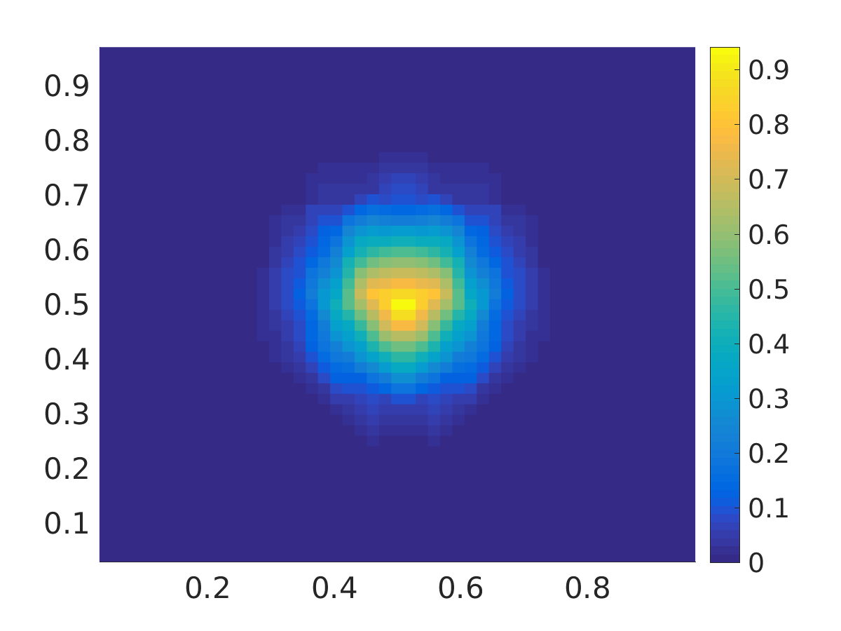
(a) Initial cancer cell density $c_{0}$

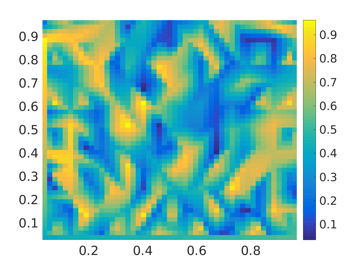
(b) Initial density $v_{0}$ of tissue fibers

Figure 1: Initial conditions

The values of the model parameters used for solving the system (2.1) are given below:

$$\kappa_{c} =10^{-3}, \kappa_{v} =1, \mu_{c} =0.5, \mu_{v} =0.02, \lambda =0.1.$$

These parameter values are in agreement with those estimated in [7]. Since cancer cells grow much faster than healthy tissue can be restructured, $\mu_{v}$ was taken to be a fraction of the cancer cell proliferation rate $\mu_{c}$.

We also perform numerical simulations for a version of the Equation (2.1a) with nondegenerate diffusion:

$$\partial_{t}\tilde{c}=\nabla\cdot\left(\frac{\kappa_{c}}{1+\tilde{v}\tilde{c}}\nabla\tilde{c}-\frac{\kappa_{v}\tilde{c}}{(1+\tilde{v})^{2}}\nabla\tilde{v}\right)+\mu_{c}\tilde{c}(1-\tilde{c}-\eta\tilde{v}) \text{ in }\mathbb{R}^{+}\times\Omega,$$

$$\partial_{t}\tilde{v}=\mu_{v}\tilde{v}(1-\tilde{v})-\lambda\tilde{v}\tilde{c} \text{ in }\mathbb{R}^{+}\times\Omega,$$

$$\frac{\kappa_{c}}{1+\tilde{v}\tilde{c}}\partial_{\nu}\tilde{c}-\frac{\kappa_{v}\tilde{c}}{(1+\tilde{v})^{2}}\partial_{\nu}\tilde{v}=0 \text{ in }\mathbb{R}^{+}\times\partial\Omega,$$

$$\tilde{c}(0)=\tilde{c}_{0}=c_{0},\ \tilde{v}(0)=\tilde{v}_{0}=v_{0} \text{ in }\Omega.$$

8.2 Results

The simulation results are shown in Figures 3 and 3. We observe that in the nondegenerate case the cancer cells are able to diffuse quite fast throughout the whole domain. In particular, the tumor cells can surpass regions of low or even (locally) vanishing ECM density and can invade their surroundings, thereby degrading the tissue in a more effective way. Due to this extended ECM deterioration flattening the fiber density profile and to the higher diffusivity throughout the domain (not restricted by gaps in the tissue), the haptotactic component of migration is outweighed by random motility. Therefore, the behavior of cancer cells with nondegenerate diffusion is much more aggressive than in the case with degenerate diffusion, where on the one hand the tumor cells are locally trapped between the regions with gaps ($v=0$) and on the other hand no diffusion takes place in the regions with $c=0$ until the tumor growth (via proliferation) did not repopulate the regions where cancer cells were lacking. Hence, cancer invasion models with nondegenerate diffusion might overestimate the extent of a tumor, especially if the latter is situated in a rather sparse tissue.

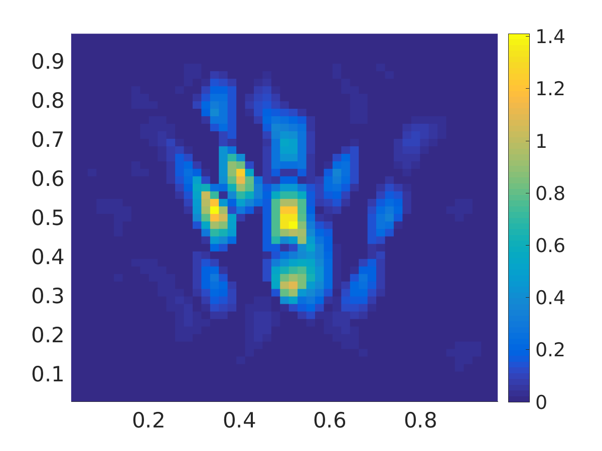
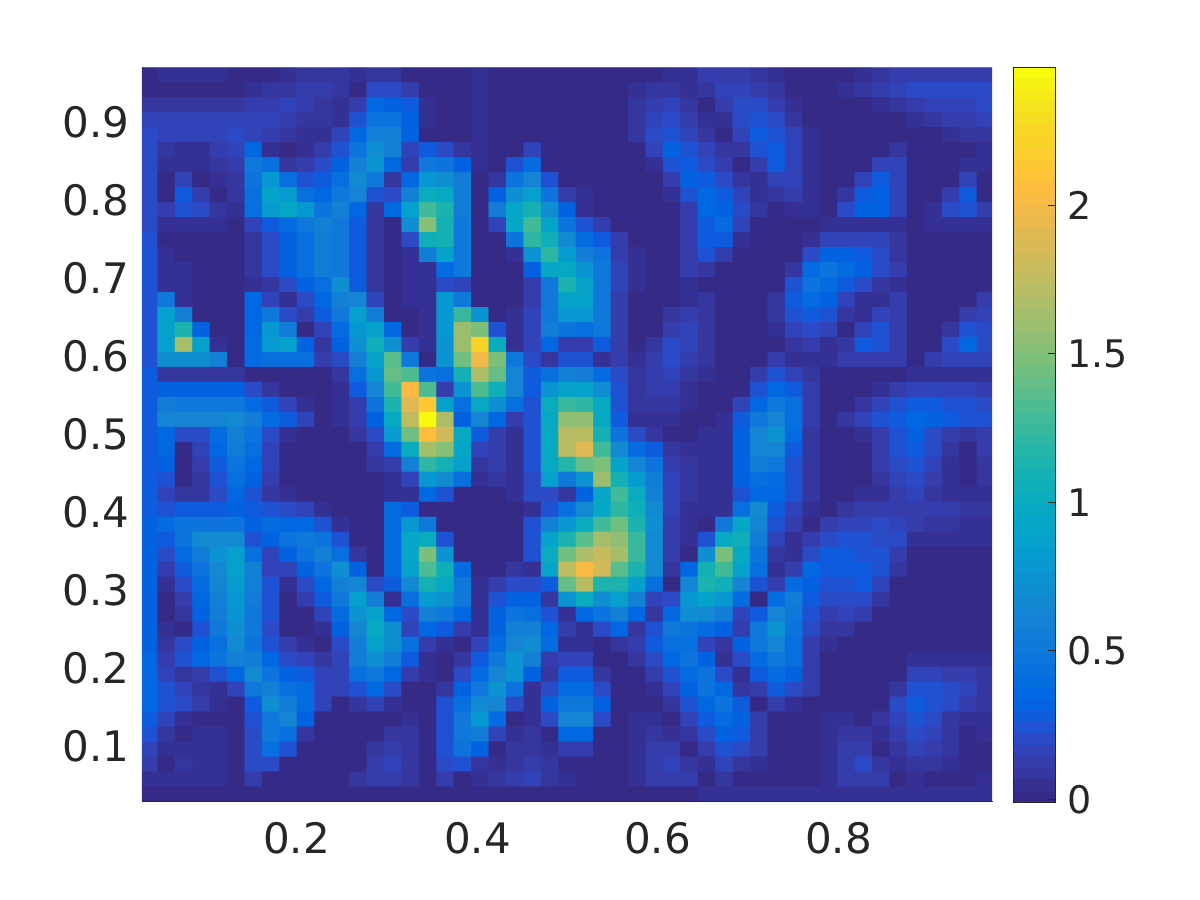
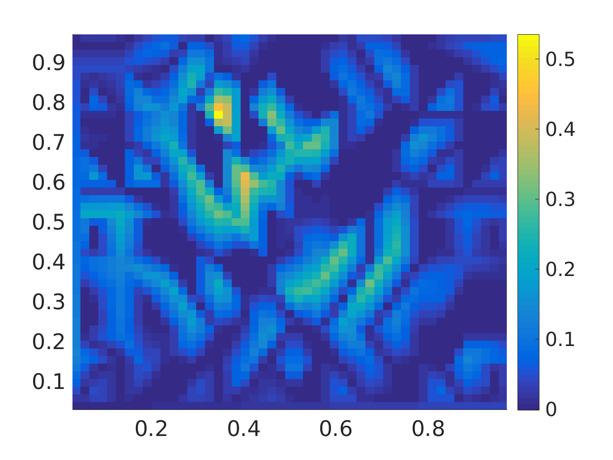
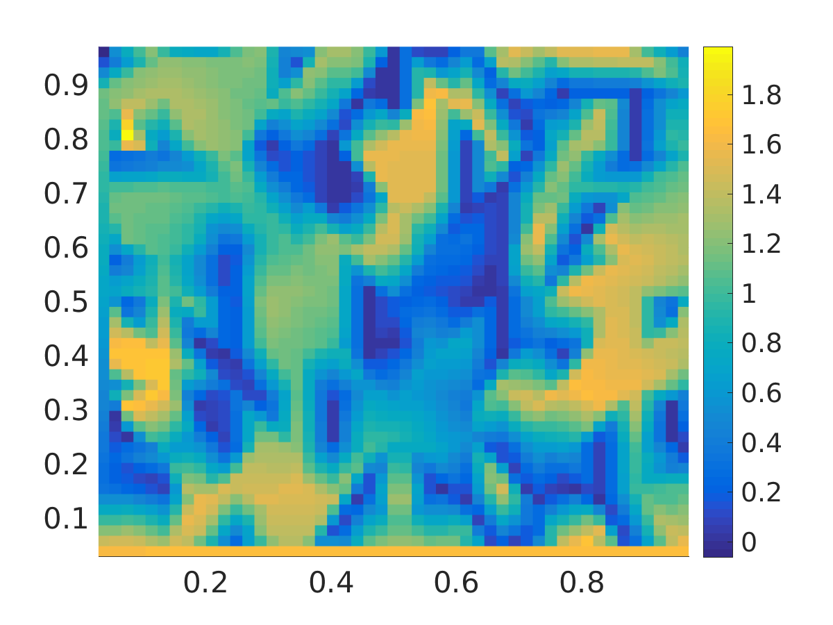
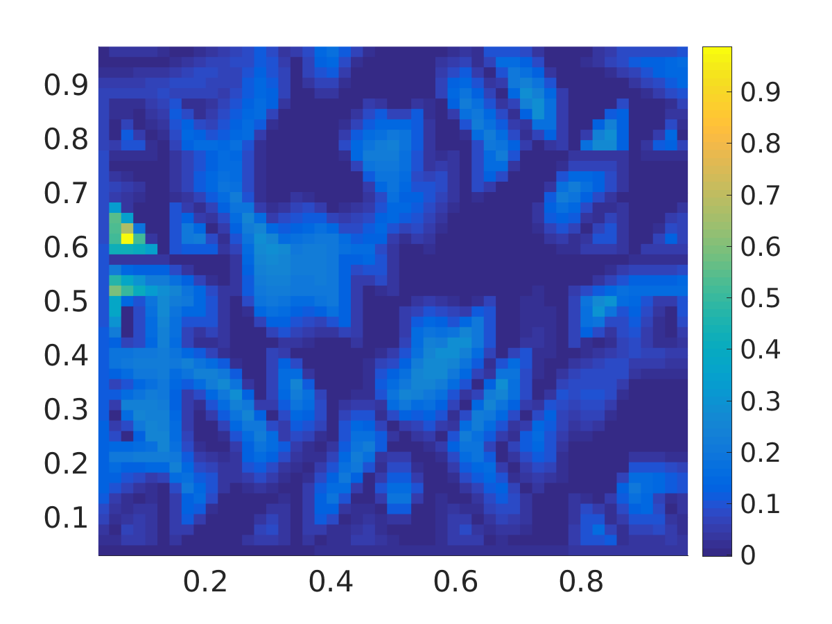
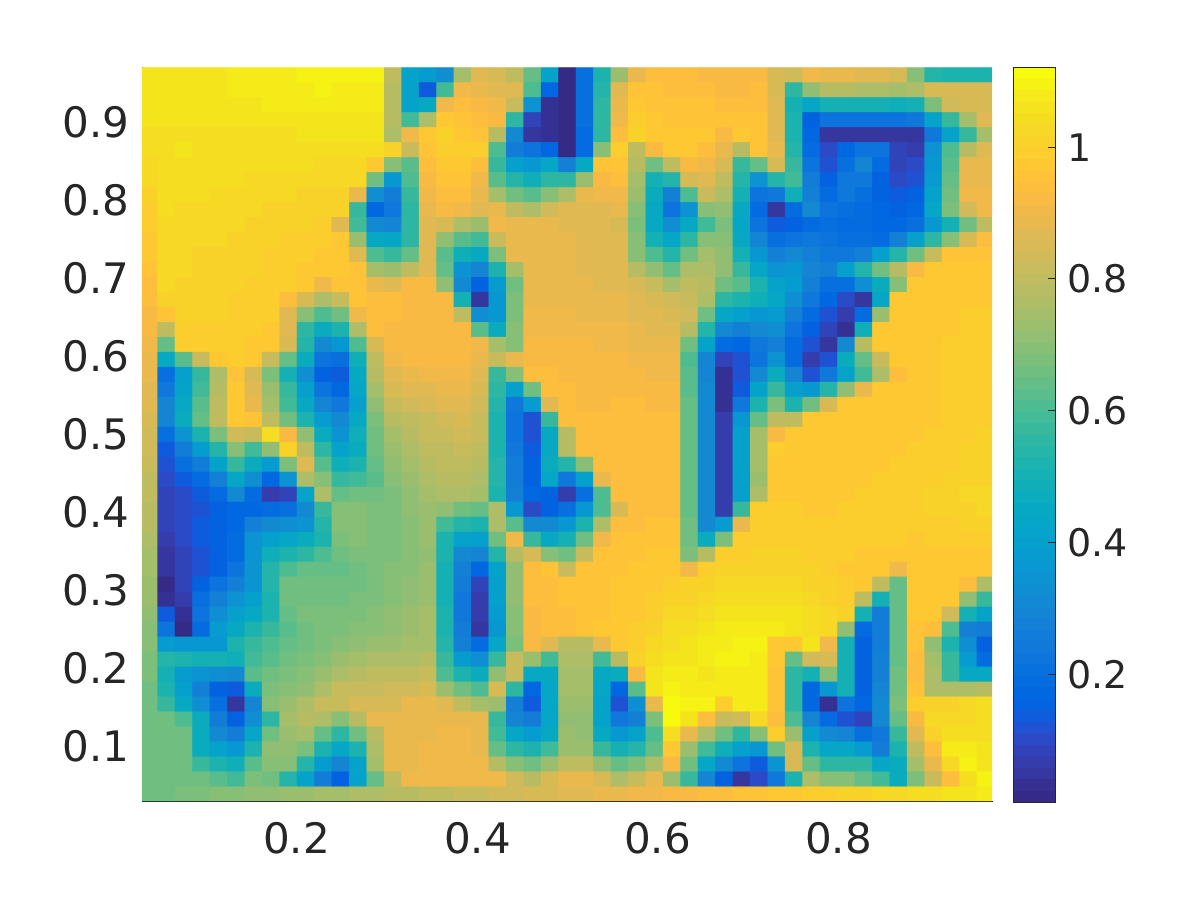
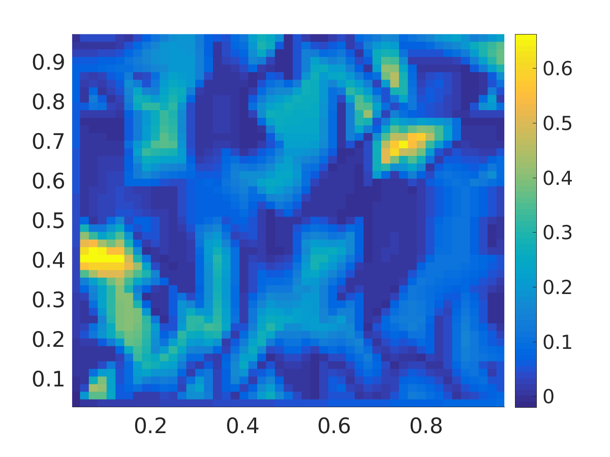
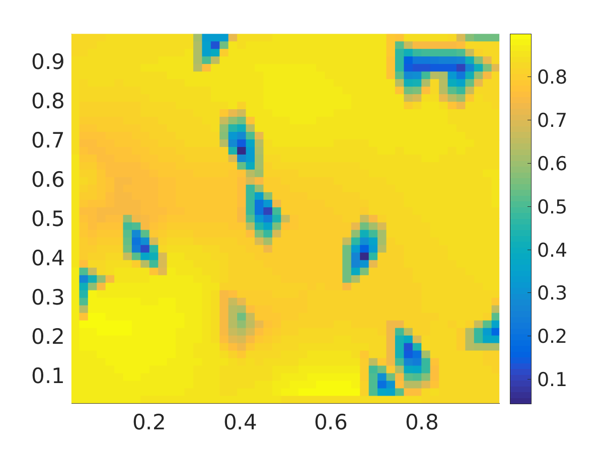
Figure 2: Simulation results for the tumor cell density with degenerate diffusion (left column) and with non-degenerate diffusion (right column) at 1, 6, 12, and 24 weeks

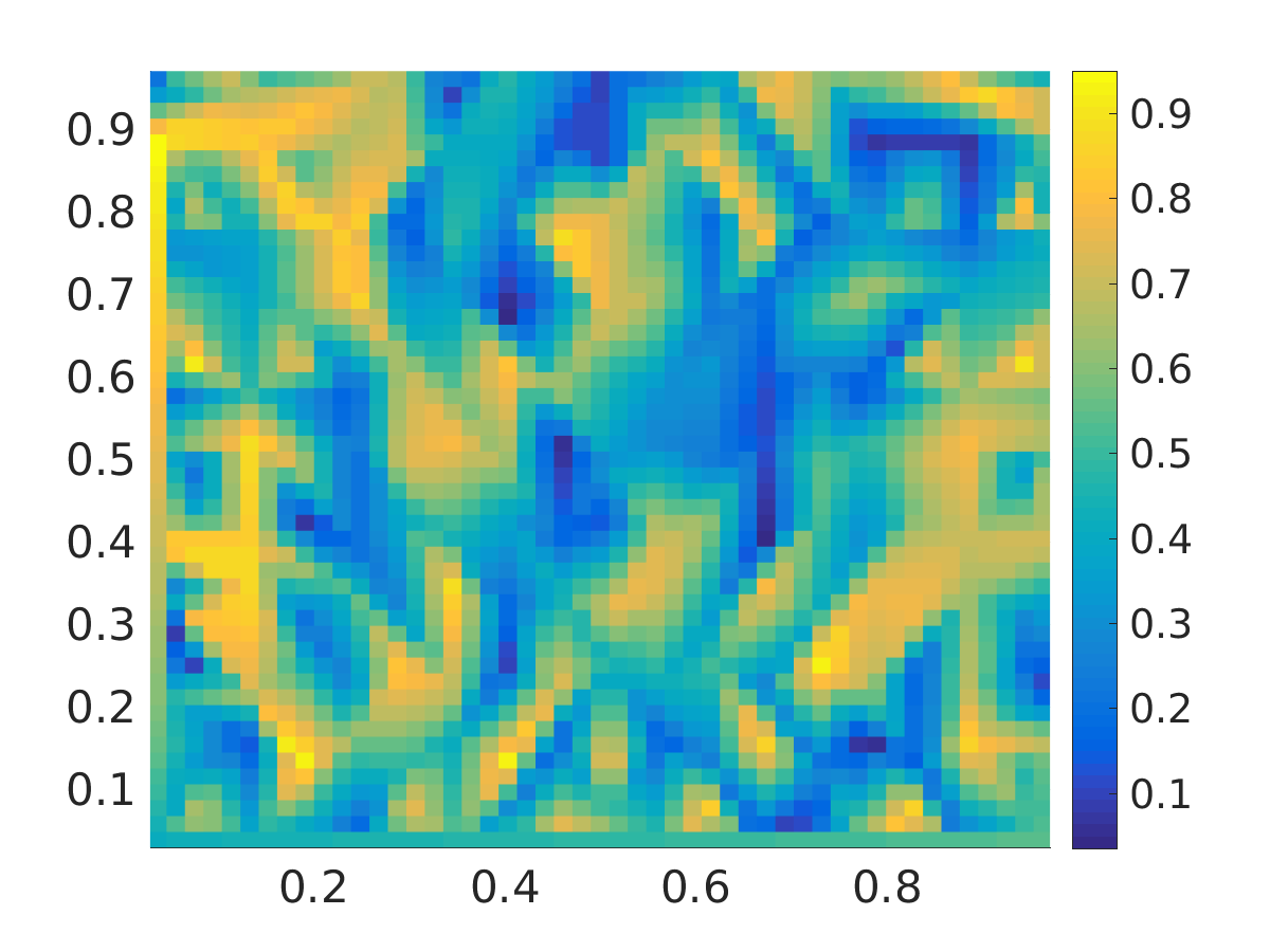
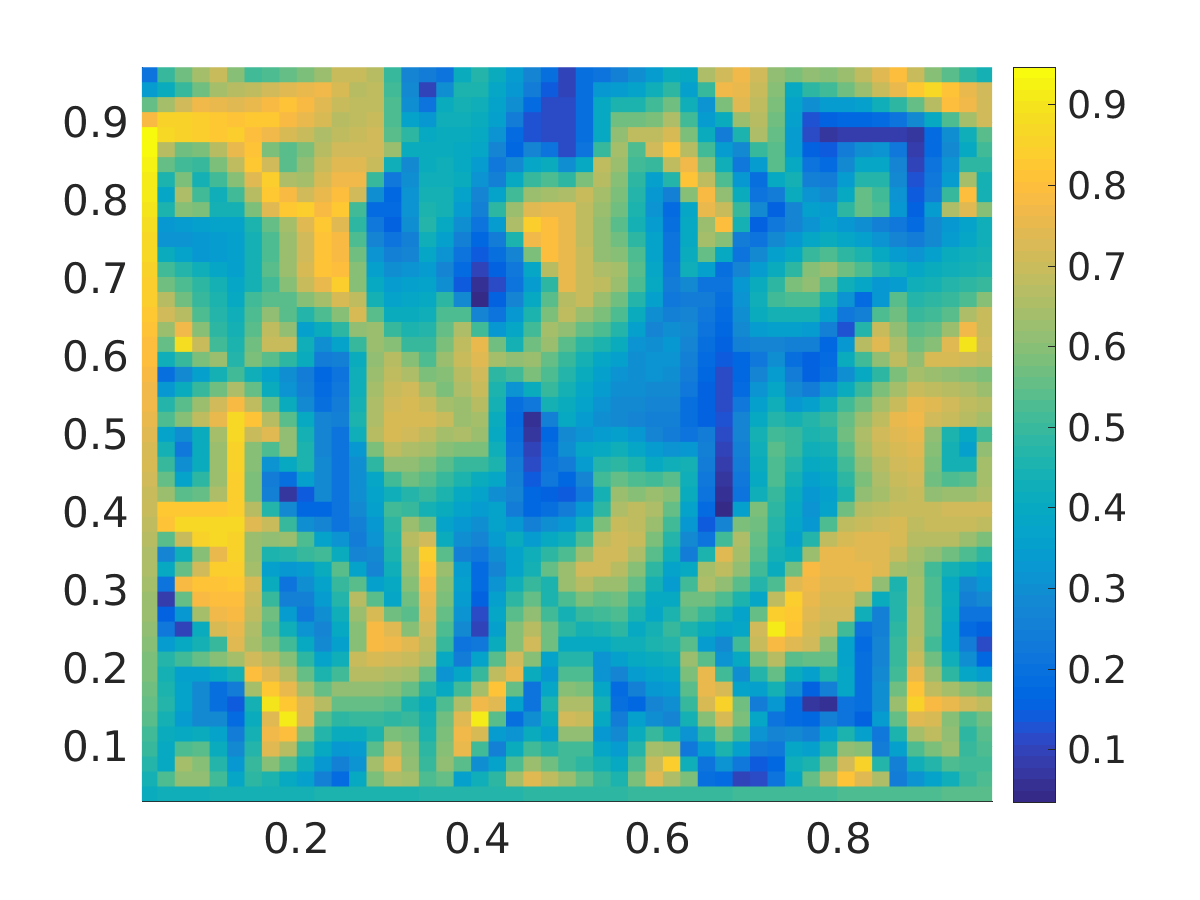
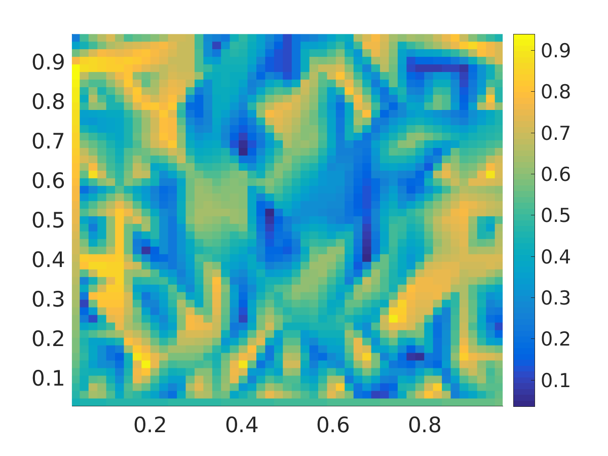
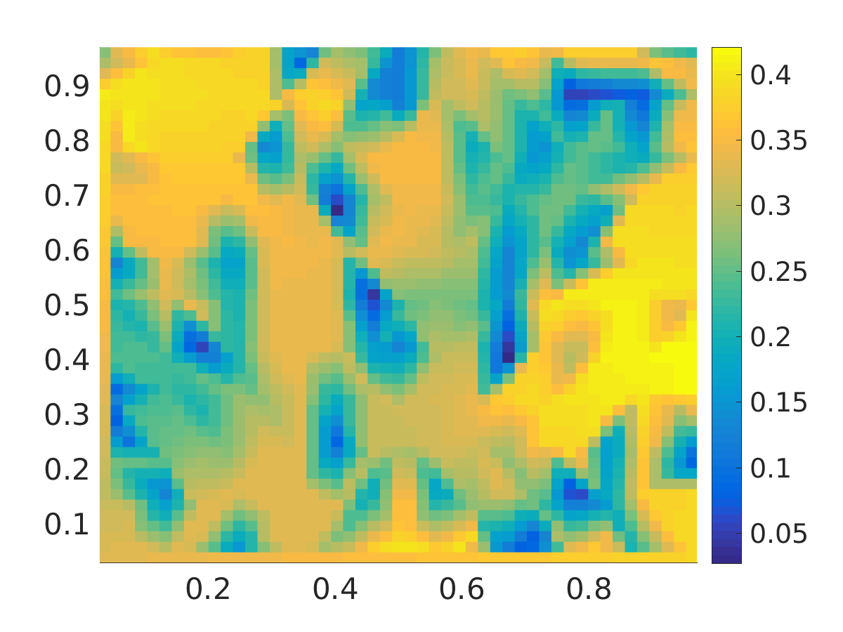
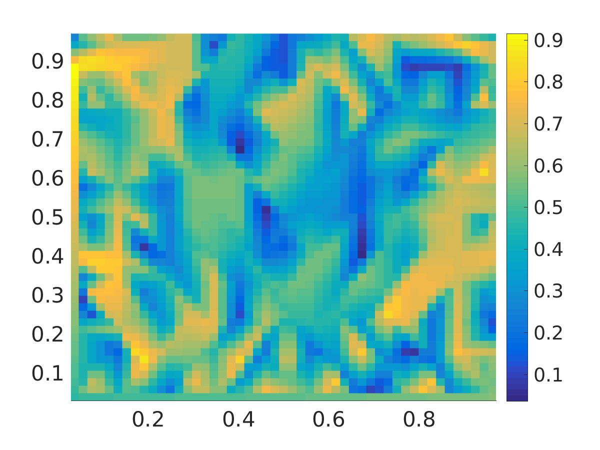
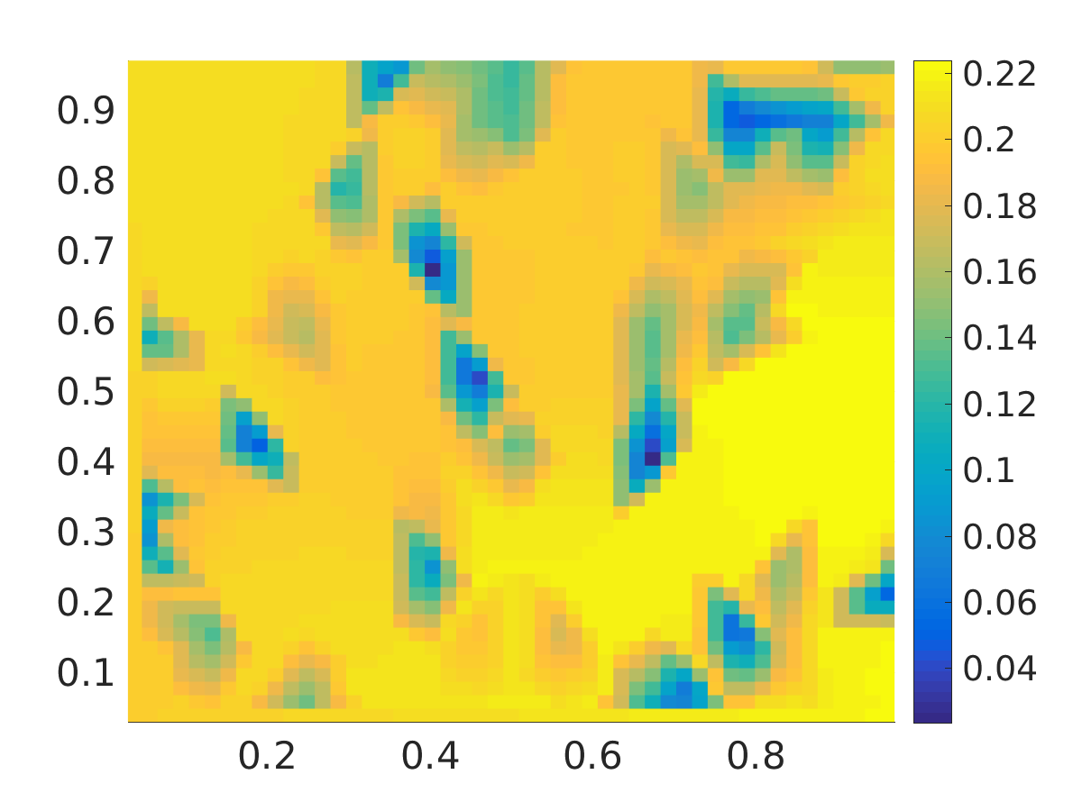
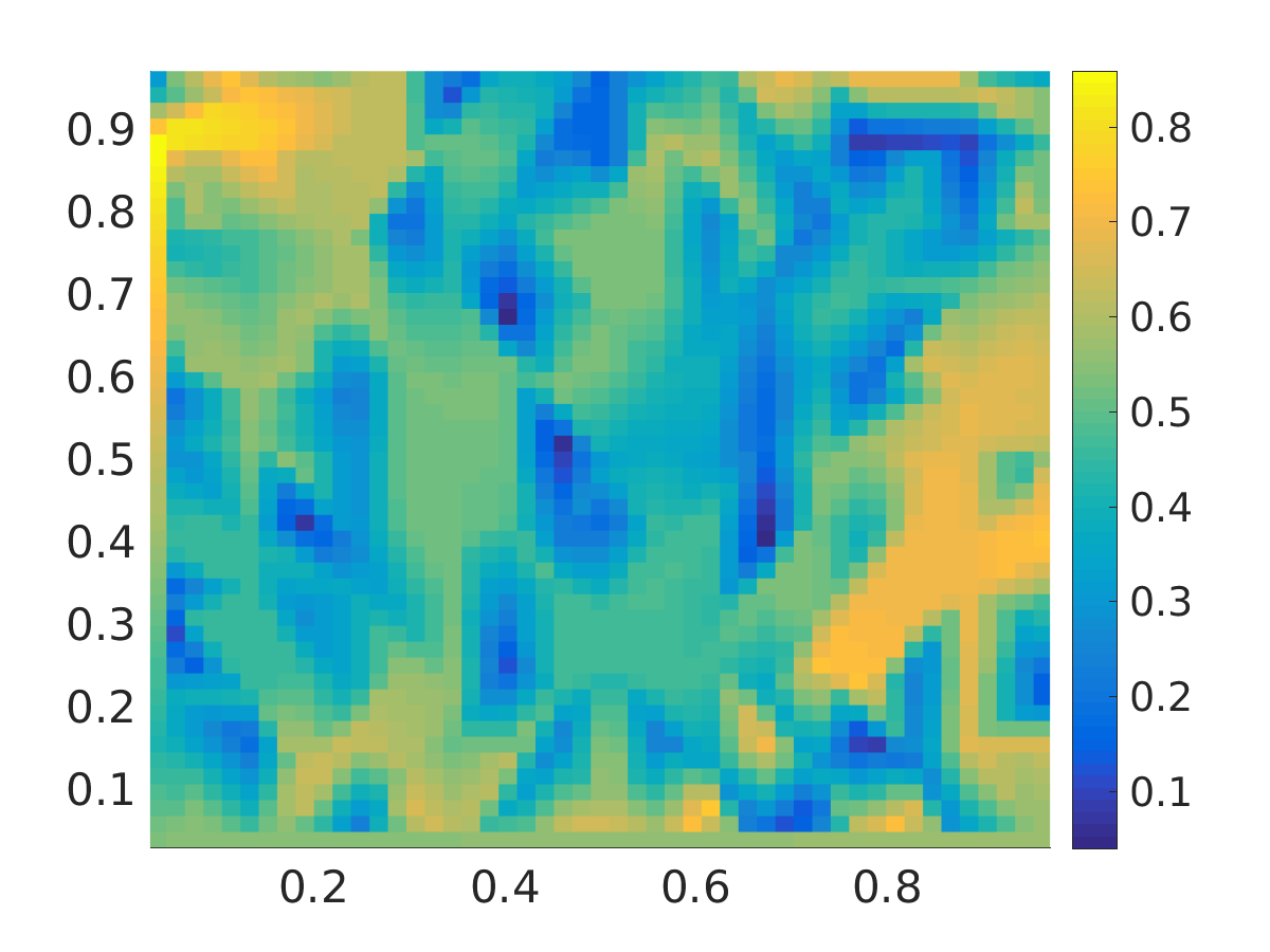
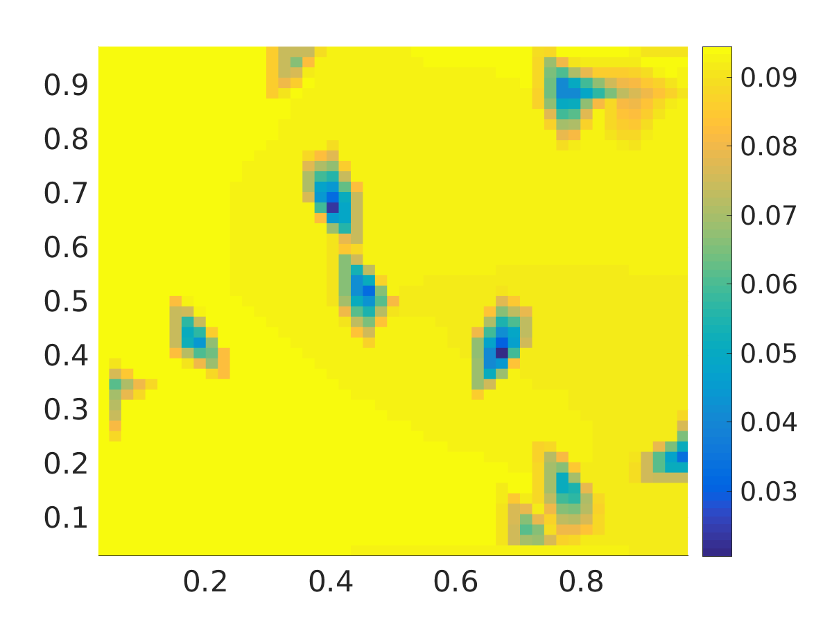
Figure 3: Simulation results for the ECM density with degenerate diffusion (left column) and with non-degenerate diffusion (right column) at 1, 6, 12, and 24 weeks

9 Discussion

We proposed a reaction-diffusion-haptotaxis model for tumor cell migration through tissue allowing for degenerate diffusion. The source of degeneracy is twofold: it can be due to the cancer cell density becoming zero and/or it can be triggered by the (locally) vanishing density of tissue fibers. Actually, both diffusion and haptotaxis terms can degenerate, but the haptotaxis coefficient can only become zero whenever the tumor cell density is vanishing. Further models with degenerate diffusion have been considered and analyzed e.g., in [39, 10, 16, 40], however, to our knowledge the present type of degeneracy is new in the context of (hapto)taxis. Particularly the presence of a possibly vanishing function $v$ in the numerator of the diffusion coefficient brought about some serious mathematical challenges, due to the absence of diffusion in the equation satisfied by the density of ECM fibers.

We proved the global existence of a solution to the higly nonlinear system coupling a PDE for the cancer cell density with an ODE for the ECM density. Precisely, Theorem 4.5 ensures the existence of at least one weak solution to (2.1). It remains open whether this solution is unique and whether there exists a solution which is globally or locally uniformly bounded.

The model in [33] involved a nondegenerate diffusion coefficient of the form $D_{c}(c,v)=\frac{\kappa}{1+cv}$, with $\kappa$ decreasing or nearly constant in time. Hence, the diffusivity was assumed there to decrease for strong interactions between cells and tissue. Here we considered a limited increase of the form $D_{c}(c,v)=\frac{\kappa_{c}cv}{1+cv}$, which can lead to the mentioned twofold degeneracy of diffusion for the tumor cells. In Section 8 we compared via simulations the behavior of haptotaxis-only models involving the two choices of diffusion coefficients . It turned out that the latter choice predicts slower invasion of the tumor and local formation of cell aggregates in the proximity of gaps in the tissue; moreover, the degradation of ECM fibers seems to be weaker with the degenerate model than with its nondegenerate counterpart. This suggests the case with degenerate diffusion is describing a less aggressive tumor behavior.

Appendix A

The following lemma is a generalisation of the Lions lemma [21, Lemma 1.3] and the known result on weak-strong convergence for member-by-member products.

Lemma A.1 (Weak-a.e. convergence).

Let $\Omega$ be a measurable subset of $\mathbb{R}^{N}$ with finite measure. Let $f,f_{n}:\Omega\rightarrow\mathbb{R}$, $n\in\mathbb{N}$ be measurable functions and $g,g_{n}\in L^{1}(\Omega)$, $n\in\mathbb{N}$. Assume further that $f_{n}\underset{n\rightarrow\infty}{\rightarrow}f$ a.e. in $\Omega$ and $g_{n}\underset{n\rightarrow\infty}{\rightharpoonup}g$, $f_{n}g_{n}\underset{n\rightarrow\infty}{\rightharpoonup}\xi$ in $L^{1}(\Omega)$. Then, it holds that $\xi=fg$ a.e. in $\Omega$.

Proof.

Since $f$ is a measurable function, the sets $\Omega_{k}:=\{|f|\leq k\}$, $k\in\mathbb{N}$, are measurable and $|\Omega\backslash\underset{k\in\mathbb{N}}{\bigcup}\Omega_{k}|=0$. Further, due to the Egorov’s theorem, there exists for each pair $k,m\in\mathbb{N}$ a measurable subset $\Omega_{k,m}$ of $\Omega_{k}$ such that $|\Omega_{k}\backslash\Omega_{k,m}|\leq\frac{1}{m}$ and $f_{n}\underset{n\rightarrow\infty}{\rightarrow}f$ uniformly in $\Omega_{k,m}$. Thus, we have that $||f||_{L^{\infty}(\Omega_{k,m})}\leq k$ and $||f_{n}-f||_{L^{\infty}(\Omega_{k,m})}\underset{n\rightarrow\infty}{\rightarrow}0$. Since $g_{n}\underset{n\rightarrow\infty}{\rightharpoonup}g$ in $L^{1}(\Omega)$, the same holds in $L^{1}(\Omega_{k,m})$. As a weakly converging sequence, $\{g_{n}\}_{n\in\mathbb{N}}$ is uniformly bounded: $\underset{n\in\mathbb{N}}{\sup}||g_{n}||_{L^{1}(\Omega_{k,m})}<\infty$. Altogether, we obtain for arbitrary $k,m\in\mathbb{N}$ and $\varphi\in L^{\infty}(\Omega_{k,m})$ that

$$\left|\int_{\Omega_{k,m}}\varphi(f_{n}g_{n}-fg)\,dx\right|\leq \left|\int_{\Omega}\varphi(f_{n}-f)g_{n}\,dx\right|+\left|\int_{\Omega_{k,m}}\varphi f(g_{n}-g)\,dx\right|$$

$$\leq ||\varphi||_{L^{\infty}(\Omega_{k,m})}\underset{n\in\mathbb{N}}{\sup}||g_{n}||_{L^{1}(\Omega_{k,m})}||f_{n}-f||_{L^{\infty}(\Omega_{k,m})}+\left|\int_{\Omega_{k,m}}\varphi f(g_{n}-g)\,dx\right|\underset{n\rightarrow\infty}{\rightarrow}0.$$

It follows that $f_{n}g_{n}\underset{n\rightarrow\infty}{\rightharpoonup}fg$ in $L^{1}(\Omega_{k,m})$. On the other hand, $f_{n}g_{n}\underset{n\rightarrow\infty}{\rightharpoonup}\xi$ in $L^{1}(\Omega)$, and, hence, also in $L^{1}(\Omega_{k,m})$. Consequently, $fg=\xi$ a.e. in $\Omega_{k,m}$ for all $k,m\in\mathbb{N}$. But $|\Omega_{k}\backslash\Omega_{m}|\leq\frac{1}{m}\underset{n^{(1)}\rightarrow\infty}{\rightarrow}0$ and $|\Omega\backslash\underset{k\in\mathbb{N}}{\bigcup}\Omega_{k}|=0$, so that $fg=\xi$ holds a.e. in $\Omega$. ∎

A similar result holds for sums of member-by-member products.

Lemma A.2 (Weak-a.e. convergence for sums).

Let $\Omega$ be a measurable subset of $\mathbb{R}^{N}$ with finite measure and let $L\in\mathbb{N}$. Let $f^{l},f^{l}_{n}:\Omega\rightarrow\mathbb{R}$, $n\in\mathbb{N}$, $l\in\{1,...,L\}$, be measurable functions and $g^{l},g^{l}_{n}\in L^{1}(\Omega)$, $n\in\mathbb{N}$, $l\in\{1,...,L\}$. Assume further that $f^{l}_{n}\underset{n\rightarrow\infty}{\rightarrow}f^{l}$ a.e. in $\Omega$ and $g^{l}_{n}\underset{n\rightarrow\infty}{\rightharpoonup}g^{l}$, $\sum_{l=1}^{L}f^{l}_{n}g^{l}_{n}\underset{n\rightarrow\infty}{\rightharpoonup}\xi$ in $L^{1}(\Omega)$. Then, it holds that $\xi=\sum_{l=1}^{L}f^{l}g^{l}$ a.e. in $\Omega$.

Remark A.3.

Observe that, in Lemma A.2, we require not the sequences $\left\{f^{l}_{n}g^{l}_{n}\right\}_{n\in\mathbb{N}}$ themselves to be convergent for $l\in\{1,...,L\}$, but only their sum $\left\{\sum_{l=1}^{L}f^{l}_{n}g^{l}_{n}\right\}_{n\in\mathbb{N}}$. Thus, the result is applicable in the cases where the convergence of individual sequences is either false or unknown.

The proof of Lemma A.2 is very similar to the proof of Lemma A.1. One only has to choose the sets $\Omega_{k}$ and $\Omega_{k,m}$ independent of $l\in\{1,...,L\}$. We leave the remaining details to the reader.

References

- [1] J.C. Adams “Regulation of protrusive and contractile cell-matrix contacts” In J. Cell Sci. 115, 2002, pp. 257–265
- [2] Herbert Amann “Linear and quasilinear parabolic problems. Vol. 1: Abstract linear theory.” Basel: Birkhäuser, 1995, pp. xxxv + 335
- [3] Herbert Amann “Nonhomogeneous linear and quasilinear elliptic and parabolic boundary value problems.” In Function spaces, differential operators and nonlinear analysis. Survey articles and communications of the international conference held in Friedrichsroda, Germany, September 20-26, 1992 Stuttgart: B. G. Teubner Verlagsgesellschaft, 1993, pp. 9–126
- [4] A.R.A. Anderson et al. “Mathematical Modelling of Tumour Invasion and Metastasis” In J. Theor. Med. 2, 2000, pp. 129–154
- [5] N.J. Armstrong, K.J. Painter and J.A. Sherratt “A Continuum Approach to Modelling Cell-Cell Adhesion” In J. Theor. Biol. 243, 2006, pp. 98–113
- [6] Timothy Barth and Mario Ohlberger “Finite Volume Methods: Foundation and Analysis” In Encyclopedia of Computational Mechanics John Wiley & Sons, Ltd, 2004 DOI: 10.1002/0470091355.ecm010
- [7] M Chaplain and G Lolas “Mathematical modelling of cancer invasion of tissue: Dynamic heterogeneity” In Netw. Heterog. Media 1, 2006, pp. 399–439
- [8] M.A.J. Chaplain and A.R.A. Anderson “Mathematical modelling of tissue invasion” In Cancer Modelling and Simulation L.Preziosi (ed.), CRC Press, 2003, pp. 269–297
- [9] M.A.J. Chaplain, M. Lachowicz, Z. Szymanska and D. Wrzosek “Mathematical Modelling of Cancer Invasion: The Importance of Cell-Cell Adhesion and Cell-Matrix Adhesion” In Math. Models Meth. Appl. Sci. 21, 2011, pp. 719–743
- [10] Hermann J. Eberl, Messoud A. Efendiev, Dariusz Wrzosek and Anna Zhigun “Analysis of a degenerate biofilm model with a nutrient taxis term.” In Discrete Contin. Dyn. Syst. 34.1 American Institute of Mathematical Sciences (AIMS), Springfield, MO, 2014, pp. 99–119 DOI: 10.3934/dcds.2014.34.99
- [11] Lawrence Craig Evans and Ronald F. Gariepy “Measure theory and fine properties of functions. 2nd revised ed.” Boca Raton, FL: CRC Press, 2015, pp. xiv + 299
- [12] Robert Eymard, Thierry Gallouët and Raphaèle Herbin “Finite volume methods” In Handbook of numerical analysis 7 Elsevier, 2000, pp. 713–1018
- [13] P. Friedl and K. Wolf “Tumor-cell invasion and migration: diversity and esacpe mechanisms” In Nature Rev. 3, 2003, pp. 362–374
- [14] A. Gerisch and M.A.J. Chaplain “Mathematical modelling of cancer cell invasion of tissue: Local and non-local models and the effect of adhesion” In J. Theor. Biol. 250, 2008, pp. 684–704
- [15] S. Hiremath and C. Surulescu “A stochastic model featuring acid induced gaps during tumor progression” In preprint, TU Kaiserslautern, submitted, 2015, pp. 1–55
- [16] Thomas Horger, Christina Kuttler, Barbara Wohlmuth and Anna Zhigun “Analysis of a bacterial model with nutrient-dependent degenerate diffusion” In Mathematical Methods in the Applied Sciences 38.17, 2015, pp. 3851–3865 DOI: 10.1002/mma.3322
- [17] K. Kawasaki et al. “Modeling Spatio-Temporal Patterns Generated byBacillus subtilis” In Journal of Theoretical Biology 188.2, 1997, pp. 177 –185 DOI: http://dx.doi.org/10.1006/jtbi.1997.0462
- [18] J. Kelkel and C. Surulescu “A Multiscale Approach to Cell Migration in Tissue Networks” In Math. Models Meth. Appl. Sci. 22, 2012, pp. 1150017–1–1150017–25
- [19] O.A. Ladyzhenskaya, V.A. Solonnikov and N.N. Ural’tseva “Linear and quasi-linear equations of parabolic type. Translated from the Russian by S. Smith.”, Translations of Mathematical Monographs. 23. Providence, RI: American Mathematical Society (AMS). XI, 648 p. (1968)., 1968
- [20] K.R. Legate, S.A. Wickström and R. Fässler “Genetic and cell biological analysis of integrin outside-in signaling” In Genes Dev. 23, 2009, pp. 397–418
- [21] J.L. Lions “Quelques méthodes de résolution des problèmes aux limites non linéaires.” Etudes mathematiques. Paris: Dunod; Paris: Gauthier-Villars. XX, 554 p. , 1969
- [22] T. Lorenz and C. Surulescu “On a class of multiscale cancer cell migration models: Well-posedness in less regular function spaces” In Math. Models Meth. Appl. Sci. 24, 2014, pp. 2383–2436
- [23] P. Lu, V.M. Weaver and Z. Werb “The extracellular matrix: A dynamic niche in cancer progression” In J. Cell Biol. 196, 2012, pp. 395–406
- [24] A. Marciniak and M. Ptashnyk “Boundedness of solutions of a haptotaxis model” In Math. Mod. Meth. Appl. Sci. 20, 2010, pp. 449–476
- [25] G. Meral, C. Stinner and C. Surulescu “On a multiscale model involvig cell contractivity and its effects on tumor invasion” In Disc. Cont. Dyn. Syst. B 20, 2015, pp. 189–213
- [26] H. Othmer and A. Stevens “Aggregation, Blowup, and Collapse: The ABCs of Taxis in Reinforced Random Walks” In SIAM J. Appl. Math. 57, 1997, pp. 1044–1081
- [27] K.J. Painter, N.J. Armstrong and J.A. Sherratt “The impact of adhesion on cellular invasion processes in cancer and development” In J. Theor. Biol. 264, 2010, pp. 1057–1067
- [28] Per-Olof Persson and Gilbert Strang “A simple mesh generator in MATLAB” In SIAM Review 46.2 SIAM, 2004, pp. 329–345
- [29] M.W. Pickup, J.K. Mouw and V.M. Weaver “The extracellular matrix modulates the hallmarks of cancer” In EMBO reports 15, 2014, pp. 1243–1253
- [30] M.A. Schwartz and R.K. Assoian “Integrins and cell proliferation: regulation of cyclin-dependent kinases via cytoplasmic signaling pathways” In J. Cell Sci. 114, 2001, pp. 2553–2560
- [31] J.A. Sherratt, S.A. Gourley, N.J. Armstrong and K.J. Painter “Boundedness of solutions of a non-local reaction-diffusion model for adhesion in cell aggregation and cancer invasion” In Eur. J. Appl. Math. 20, 2009, pp. 123–144
- [32] Jacques Simon “Compact sets in the space .” In Ann. Mat. Pura Appl. (4) 146 Springer, Berlin/Heidelberg; Fondazione Annali di Matematica Pura ed Applicata c/o Dipartimento di Matematica “U. Dini”, Firenze, 1987, pp. 65–96 DOI: 10.1007/BF01762360
- [33] Christian Stinner, Christina Surulescu and Michael Winkler “Global weak solutions in a PDE-ODE system modeling multiscale cancer cell invasion.” In SIAM J. Math. Anal. 46.3 Society for IndustrialApplied Mathematics (SIAM), Philadelphia, PA, 2014, pp. 1969–2007 DOI: 10.1137/13094058X
- [34] Z. Szymanska, C. Morales-Rodrigo, M. Lachowicz and M.A.J. Chaplain “Mathematical Modelling of Cancer Invasion of Tissue: The Role and Effect of Nonlocal Interactions” In Math. Models Meth. Appl. Sci. 19, 2009, pp. 257–281
- [35] Y. Tao and M. Wang “Global existence of classical solutions to a combined chemotaxis-haptotaxis model with logistic source” In J. Math. Anal. Appl. 354, 2009, pp. 60–69
- [36] Y. Tao and M. Winkler “A chemotaxis-haptotaxis model: the roles of nonlinear diffusion and logistic source” In SIAM J. Math. Anal. 43, 2011, pp. 685–705
- [37] C. Walker and G.F. Webb “Global existence of classical solutions for a haptotaxis model” In SIAM J. Math. Anal. 38, 2007, pp. 1694–1713
- [38] Y. Wang “Boundedness in the higher dimensional chemotaxis-haptotaxis model with nonlinear diffusion” In J. Diff. Equations 260, 2016, pp. 1975–1989
- [39] Zhi-An Wang, Michael Winkler and Dariusz Wrzosek “Global regularity versus infinite-time singularity formation in a chemotaxis model with volume-filling effect and degenerate diffusion.” In SIAM J. Math. Anal. 44.5 Society for IndustrialApplied Mathematics (SIAM), Philadelphia, PA, 2012, pp. 3502–3525 DOI: 10.1137/110853972
- [40] P. Zheng, C. Mu and X. Song “On the boundedness and decay of solutions for a chemotaxis-haptotaxis system with nonlinear diffusion” In Discr. Cont. Dyn. Syst. A 36, 2016, pp. 1737 –1757