A weighted extended B-spline solver for bending and buckling of stiffened plates

Abstract

The weighted extended B-spline method [Höllig (2003)] is applied to bending and buckling problems of plates with different shapes and stiffener arrangements. The discrete equations are obtained from the energy contributions of the different components constituting the system by means of the Rayleigh-Ritz approach. The pre-buckling or plane stress is computed by means of Airy’s stress function. A boundary data extension algorithm for the weighted extended B-spline method is derived in order to solve for inhomogeneous Dirichlet boundary conditions. A series of benchmark tests is performed touching various aspects influencing the accuracy of the method.

1 Introduction

The growing need for larger container ships [1] led to renewed interest in computational methods for plate bending and plate buckling in the maritime industry. One of the main challenges in the construction of modern container vessels is to provide a sufficient ultimate strength of the structure while keeping the material usage minimal. The development of more accurate and faster computational methods is one aspect in helping the industry obtaining these goals.

The physics and methods for plate bending and buckling problems with stiffener arrangements are treated and reviewed in [2, 3, 4, 5]. There is a relatively long history on the numerical treatment of the plate bending and buckling equations, for which the finite element method [6, 7, 8, 9], the boundary element method [10, 11, 12], the finite strip method [13] and the quadrature element method [14] probably account for the most widespread methods. Another class of methods are the sometimes called semi-analytic methods based on Navier’s sine solution. Among these we find the method by [15] for rectangular plates and stiffener arrangements and the one by [16] for buckling of plates of more complex geometries. As a method, which is more related to the present work, B-splines have been in use for plate deformation, vibration and buckling problems, for example for rectangular domains [17, 18, 19, 20] or in connection with the isoparametric stripe approach for more complicated geometries [21, 22]. A general trend in computational solid mechanics is the integration between CAD and structural analysis, which has led to the usage of B-splines in connection with NURBS for the isogeometric approach. The isogeometric approach with NURBS has also been used for plate bending problems [23, 24, 25, 26, 27, 28, 29].

On the other hand, the weighted extended B-spline method [30] follows a similar aim as the isogeometric approach with NURBS, namely to facilitate the integration between CAD and structural analysis. Whereas the isogeometric approach is based on using the same discretization for the structural analysis as for the CAD, the weighted extended B-spline method aims to facilitate integration of CAD and structural solver by describing the boundary of the domain in an embedded fashion, allowing for a flexible treatment of complicated geometries, while leading to sparse matrices and being higher order accurate.

As such, a single example of bending of a clamped plate has been solved in [30] by means of the weighted extended B-spline method. In the present treatise this method is applied to the bending and buckling problem of Kirchhoff plates of various shapes with and without stiffeners. Using the energy formulation of the system, the Rayleigh-Ritz approach is used to obtain the discrete equations. The pre-buckling stress is computed by means of Airy’s stress function. A scheme to solve for inhomogeneous Dirichlet boundary conditions in the framework of the weighted extended B-spline method is derived in order to handle the traction boundary conditions for Airy’s stress function. The method is applied to a number of benchmark cases. Thereby different issues affecting the accuracy, such as discontinuities or singularities, are discussed. As the method displays higher order accuracy, it is particularly well adapted for eigenvalue problems [31] as arising in plate buckling.

The present work is organized as follows. In section 2, the physical problem is presented. The weighted extended B-spline method by [30] is briefly summarized in section 3. In this section, we shall also explain the adaptation of the weighted extended B-spline method to the present computation of the plate bending and buckling problem and the pre-buckling stress. Results for a number of benchmark cases are presented in section 4. The present treatise is concluded in section 5.

2 Physical problem

2.1 Bending and buckling of plate and stiffener

In figure 1, the geometry of a plate is sketched. It is described by a domain $\Omega\subset\mathbb{R}^{2}$ not necessarily simply connected (we allow for holes). At the straight line $\Gamma$, a stiffener is attached to the plate. For the domain $\Omega$, we use the coordinate system given by $(x,y,z)$. The orientation of the stiffener gives rise to a coordinate system defined by $(\zeta,\eta,\theta)$, where $\theta$ is the arclength. The $\theta$-axis is parallel to the stiffener, whereas $(\zeta,\eta)$ are in the plane perpendicular to the axis of the stiffener with the $\zeta$-axis lying in the $(x,y)$ plane of the plate. For a Kirchhoff plate, the displacement of the middle surface of the plate is entirely described by the vertical displacement $w$. The bending energy $U_{plate}$ of a Kirchhoff plate is then given by [3]:

$$U_{plate}=\frac{D}{2}\int\limits_{\Omega}\left(\nabla^{2}w\right)^{2}-2\left(1-\nu\right)\left\{\frac{\partial^{2}w}{\partial x^{2}}\frac{\partial^{2}w}{\partial y^{2}}-\left(\frac{\partial^{2}w}{\partial x\partial y}\right)^{2}\right\}d\,\Omega$$ (1)

If a distribution $p(x,y)$ of lateral forces per area is applied to the plate, the work $W_{lateral}$ done by these lateral forces has to be added to the total energy,

$$W_{lateral}=-\int\limits_{\Omega}pw\,d\Omega.$$ (2)

On the other hand, when considering buckling, in-plane forces $\mathbf{T}$ are applied at the boundary $\partial\Omega$ of the plate. These forces $\mathbf{T}=(T_{x},T_{y})$ give rise to a stress field $\sigma$ in the plate which shall be called the pre-buckling stress field and whose computation shall be described in section 2.2. Once the plate buckles, the work $W_{buckling}$ done by the in-plane forces can be computed by [3]:

$$W_{buckling}=\frac{1}{2}\int\limits_{\Omega}\sigma_{xx}\left(\frac{\partial w}{\partial x}\right)^{2}+\sigma_{yy}\left(\frac{\partial w}{\partial y}\right)^{2}+2\sigma_{xy}\frac{\partial w}{\partial x}\frac{\partial w}{\partial y}\,d\Omega.$$ (3)

Equations (1-3) describe all the relevant energy contributions for plate bending and buckling without stiffeners. Since at $\Gamma$, cf. figure 1, a stiffener is attached to the plate, its energy contribution needs to be added to the total energy of the system. In the present discussion, the cross-section of the stiffener is assumed to stay constant during deformation. For a class of stiffeners the torsional and warping energies are negligible compared to the bending energy. The present discussion is restricted to these type of stiffeners. The displacement of the stiffener is thus in vertical direction of an equal amount as the plate, since no detachment of the stiffener is allowed. The bending energy of the stiffener can then be written as:

$$U_{stiffener}=\frac{EI}{2}\int\limits_{\Gamma}\left(\frac{d^{2}w}{d\theta^{2}}\right)^{2}\,d\theta,$$ (4)

where $EI$ is the bending stiffness in vertical direction of the stiffener. If opposing forces of equal magnitude $T_{s}$ are applied at both ends in axial direction of the stiffener, the work $W_{stiffener}$ due to axial shorting of the stiffener needs to be accounted for. According to [4] (formula 5.42), $W_{stiffener}$ can in our case be written as:

$$W_{stiffener}=\frac{T_{s}}{2}\int\limits_{\Gamma}\left\{\left(\frac{dw}{d\theta}\right)^{2}+r_{0}^{2}\left(\frac{d}{d\theta}\frac{\partial w}{\partial\zeta}\right)^{2}-2\zeta_{0}\frac{dw}{d\theta}\left(\frac{d}{d\theta}\frac{\partial w}{\partial\zeta}\right)\right\}\,d\theta,$$ (5)

where $r_{0}$ is the radius of gyration and $\zeta_{0}$ the $\zeta$-coordinate of the centroid of the cross section:

$$Ar_{0}=\int\limits_{A}(\zeta^{2}+\eta^{2})\,d\zeta d\eta,\quad A\zeta_{0}=\int\limits_{A}\zeta\,d\zeta d\eta,$$ (6)

where $A$ is the area of the cross section.

Having defined all the relevant energy contributions, the problem of plate bending by lateral loads and of plate buckling by in-plane loads can be defined as follows.

Plate bending

When lateral loads are applied, the plate and the stiffener undergo bending and the total energy $E_{bending}$ of the system can be written as:

$$E_{bending}=U_{plate}+U_{stiffener}+W_{lateral}.$$ (7)

The governing equations of the system can be obtained by variational minimization of (7). For the present system, we obtain:

$$D\nabla^{4}w = p\quad\mbox{in}\quad\Omega\setminus\Gamma,$$ (8)

$$D\left[\lim_{\epsilon\rightarrow 0^{+}}\frac{\partial^{3}w}{\partial\zeta^{3}}-\lim_{\epsilon\rightarrow 0^{-}}\frac{\partial^{3}w}{\partial\zeta^{3}}\right]+EI\frac{\partial^{4}w}{\partial\theta^{4}} = 0\quad\mbox{on}\quad\Gamma,$$ (9)

in addition to boundary conditions on the boundary of $\Omega$.

Plate buckling

When in-plane loads are applied, the plate and the stiffener undergo sudden buckling once a critical value of the loading has been reached. The energy $E_{buckling}$ of the problem is given by:

$$E_{buckling}=U_{plate}+U_{stiffener}+\lambda\left(W_{buckling}+W_{stiffener}\right),$$ (10)

where $\lambda$ is a parameter controlling the intensity of the in-plane loading. In the framework of small displacement theory, it plays the role of an eigenvalue allowing for non-trivial solutions of $w$ minimizing equation (10).

2.2 Pre-buckling stress

As mentioned above, the pre-buckling stress enters equation (3) and is unknown a priory. A weighted extended B-spline formulation for the plane stress problem in terms of the horizontal displacements can be found in [30]. However, in the present case, the boundary conditions are given in terms of the in-plane forces $\mathbf{T}$ at the boundaries of $\Omega$ which result into boundary conditions for the stress tensor $\sigma$. The horizontal displacements at the boundaries are unknown a priori and the formulation in [30] cannot be applied straightforwardly. As such iterative solvers might be applied accounting for the undetermined solid body motions. However, as we are employing a direct solver, a more practical approach is to use the Airy stress function formulation. The present plane stress problem is therefore expressed in terms of Airy’s stress function $\Phi$. When dealing with multiple connected domains, a necessary condition for the Airy stress function to exist and to be smooth is that the total force and torque at the outer boundary and at the boundary of each hole vanishes separately [32]. In the present context, free holes, i.e. absence of traction, are of main interest, such that the Airy stress function formulation is applicable.

The stress components are expressed via Airy’s stress function as:

$$\sigma_{xx}=\frac{\partial^{2}\Phi}{\partial y^{2}}\quad\sigma_{yy}=\frac{\partial^{2}\Phi}{\partial x^{2}}\quad\sigma_{xy}=-\frac{\partial^{2}\Phi}{\partial y\partial x},$$ (11)

and the traction boundaries can be written as

$$T_{x} = \frac{d}{ds}\frac{\partial\Phi}{\partial y}$$ (12)

$$T_{y} = -\frac{d}{ds}\frac{\partial\Phi}{\partial x},$$ (13)

where $s$ is the arclength of the boundary. When the domain is multiply connected by $n+1$ boundaries, i.e. one outer boundary and $n$ inner boundaries (holes), the boundary conditions (12) and (13) translate to the following expressions for each boundary $\partial\Omega_{i}$, $i=0,\ldots,n$ [33]:

$$\left.\begin{array}[]{lcl}\Phi&=&\gamma_{i}+\alpha_{i}x+\beta_{i}y+F_{i}\\ \frac{\partial\Phi}{\partial n}&=&\alpha_{i}n_{x}+\beta_{i}n_{y}+N_{i}\end{array}\right\}\quad\mbox{for}\quad(x,y)\in\partial\Omega_{i},$$ (14)

where $\alpha_{i}$, $\beta_{i}$ and $\gamma_{i}$ are constants of integration, $n_{x}$ and $n_{y}$ are the components of the outward pointing normal on the boundary $\partial\Omega_{i}$ and the functions $F_{i}$ and $N_{i}$ are defined as follows:

$$F_{i}(s) = \int\limits_{0}^{s}\frac{dx}{ds}(s^{\prime})f_{x}(s^{\prime})+\frac{dy}{ds}(s^{\prime})f_{y}(s^{\prime})\,ds^{\prime}$$ (15)

$$N_{i}(s) = \frac{dy}{ds}(s)f_{x}(s)-\frac{dx}{ds}(s)f_{y}(s)$$ (16)

$$f_{x}(s) = -\int\limits_{0}^{s}T_{y}(s^{\prime})\,ds^{\prime}$$ (17)

$$f_{y}(s) = \int\limits_{0}^{s}T_{x}(s^{\prime})\,ds^{\prime}$$ (18)

In terms of Airy’s stress function, the membrane energy $E_{m}$ of the plate becomes:

$$E_{m}[\Phi] = \frac{h}{2E}\int\limits_{\Omega}\left(\Delta\Phi\right)^{2}+2(1+\nu)\left\{\left(\frac{\partial^{2}\Phi}{\partial x\partial y}\right)^{2}-\frac{\partial^{2}\Phi}{\partial x^{2}}\frac{\partial^{2}\Phi}{\partial y^{2}}\right\}\,d\Omega$$ (19)

$$= \frac{h}{2E}\int\limits_{\Omega}\left(\Delta\Phi\right)^{2}\,d\Omega-\frac{h}{2E}\sum\limits_{i=0}^{n}\int\limits_{\partial\Omega_{i}}f_{x}T_{x}+f_{y}T_{y}\,d\sigma$$ (20)

where $f_{x}$ and $f_{y}$ are defined in equations (17) and (18), respectively. The second term in equation (20) is just a constant. An equivalent energy $E^{*}_{m}$ for $\Phi$ can therefore be written as:

$$E_{m}^{*}[\Phi]=\int\limits_{\Omega}\left(\Delta\Phi\right)^{2}\,d\Omega,$$ (21)

which after variational minimization leads to

$$\Delta^{2}\Phi=0\quad\mbox{in}\quad\Omega.$$ (22)

Equation (22) tells us that the method of choice for the plane stress problem would be a boundary integral or boundary element solver [33], since it would reduce the two-dimensional problem into a one-dimensional one. The resulting stress field could then be fed to the solver presented in section 3 in order to solve the buckling problem (10). However, for illustration purposes we shall use the present solver in order to solve the plane stress problem for Airy’s stress function, since it shows how inhomogeneous Dirichlet boundary conditions can be handled in the framework of the weighted extended B-spline method.

When given a multiple connected domain, with $n+1$ boundaries, we shall solve $4(n+1)$ times the following decoupled problems:

$$\Delta^{2}\Phi_{ik} = 0\quad x\in\Omega\quad i=0,\ldots,n\quad k=0,\ldots,3$$ (23)

with the following boundary conditions:

$$\Phi_{i0} = F_{i},\quad\frac{\partial\Phi_{i0}}{\partial n}=N_{i}\quad x\in\partial\Omega_{i}$$ (24)

$$\Phi_{i1} = 1,\quad\frac{\partial\Phi_{i1}}{\partial n}=0\quad x\in\partial\Omega_{i}$$ (25)

$$\Phi_{i2} = x,\quad\frac{\partial\Phi_{i2}}{\partial n}=n_{x}\quad x\in\partial\Omega_{i}$$ (26)

$$\Phi_{i3} = y,\quad\frac{\partial\Phi_{i3}}{\partial n}=n_{y}\quad x\in\partial\Omega_{i}$$ (27)

$$\Phi_{ik} = 0,\quad\frac{\partial\Phi_{ik}}{\partial n}=0\quad x\in\partial\Omega_{j}\quad\forall j\neq i\quad k=0,\ldots,3.$$ (28)

The linear combination

$$\Phi=\sum\limits_{i=0}^{n}\Phi_{i0}+\gamma_{i}\Phi_{i1}+\alpha_{i}\Phi_{i2}+\beta_{i}\Phi_{i3},$$ (29)

satisfies the governing equation (22) and the boundary conditions (12) and (13).

In the framework of the boundary integral or boundary element method [33] constraints for the undetermined constants $\alpha_{i}$, $\beta_{i}$, $\gamma_{i}$, $i=0,\ldots,n$ can be formulated exploiting compatibility between displacements and stresses. However, for a volume based method (or area based in two dimensions) as the present method, such an approach is not straightforward. We shall instead use the minimum energy principle by writing:

$$E^{*}_{m}[\Phi] = E^{*}_{m}\left[\sum\limits_{i=0}^{n}\Phi_{i0}+\gamma_{i}\Phi_{i1}+\alpha_{i}\Phi_{i2}+\beta_{i}\Phi_{i3}\right]$$ (30)

$$= E^{*}_{m}(\dots,\alpha_{i},\beta_{i},\gamma_{i},\ldots)$$ (32)

$$= \sum\limits_{i=0}^{n}\sum\limits_{j=0}^{n}\int\limits_{\Omega}\left(\Delta\Phi_{i0}+\gamma_{i}\Delta\Phi_{i1}+\alpha_{i}\Delta\Phi_{i2}+\beta_{i}\Delta\Phi_{i3}\right)$$

$$\quad\quad\left(\Delta\Phi_{j0}+\gamma_{j}\Delta\Phi_{j1}+\alpha_{j}\Delta\Phi_{j2}+\beta_{j}\Delta\Phi_{j3}\right)\,d\Omega$$

The coefficients $\alpha_{i}$, $\beta_{i}$, $\gamma_{i}$, $i=0,\ldots,i$ are then found by minimizing the function $E^{*}_{m}(\dots,\alpha_{i},\beta_{i},\gamma_{i},\ldots)$ under the constraint that

$$\int\limits_{\Omega}\Phi\,d\Omega = 0,$$ (33)

$$\int\limits_{\Omega}\frac{\partial}{\partial x}\Phi\,d\Omega = 0,$$ (34)

$$\int\limits_{\Omega}\frac{\partial}{\partial y}\Phi\,d\Omega = 0,$$ (35)

since any function of the form:

$$\Phi+a+bx+cy,$$ (36)

where $a$, $b$ and $c$ are arbitrary constants, satisfies equations (12), (13) and (22).

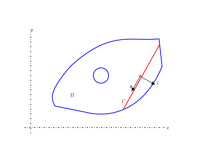
Figure 1: A plate $\Omega$ with a stiffener connected to the plate at $\Gamma$.

3 Numerical scheme

This section presents briefly the main results of the weighted extended B-spline method, presented in detail in [34, 30, 35, 36]. The weighted extended B-spline method is a finite element method based on B-splines combined with an embedded description of the boundary. The method can be considered a Cartesian grid method, which avoids grid generation, since no body fitted mesh needs to be generated. The vertical displacement $w$ of the plate is expanded on the weighted extended B-spline basis functions $B_{\mathbf{k}}$ [30]:

$$w=\sum\limits_{\mathbf{i}\in\mathcal{I}}w_{\mathbf{i}}B_{\mathbf{i}}(x,y),$$ (37)

where $\mathbf{i}=(i_{x},i_{y})$ is a two-dimensional index which can be mapped onto a global index $i$. The set $\mathcal{I}$ denotes the set of inner indices, which shall be explained below. The construction of the weighted extended B-spline basis functions shall now be presented along general lines, for details we refer to [30].

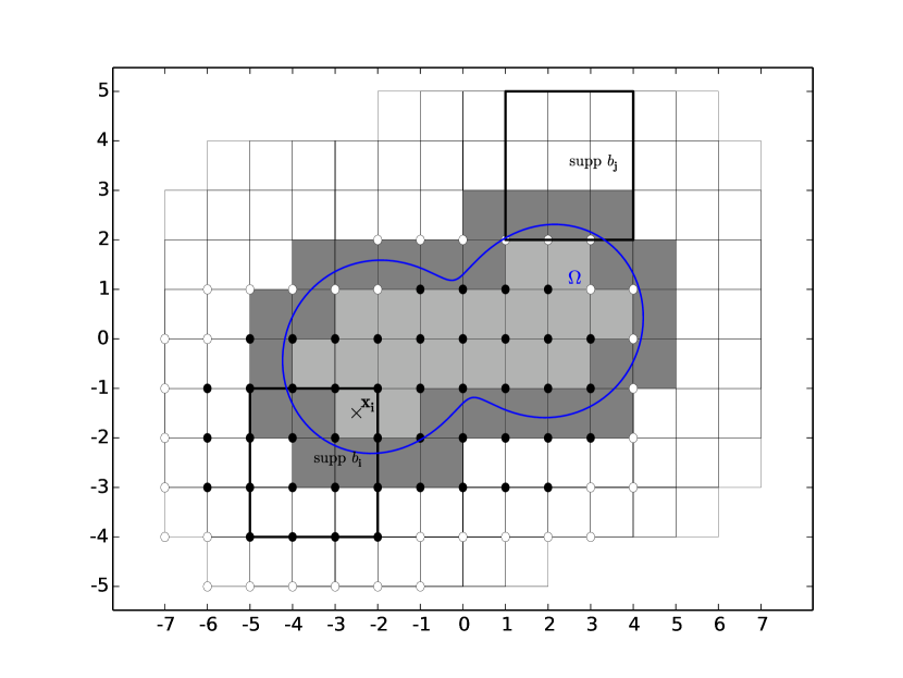
Figure 2: Discretization of a domain $\Omega$. The boundary of $\Omega$ (blue line) is embedded in a grid consisting of uniform rectangular cells. Cells can either be cut by the boundary (boundary cells, dark gray color), lie completely inside the domain (interior cells, light gray color) or lie outside of the domain (exterior cells, white color).

The discretization of a two dimensional domain $\Omega$ is given by square cells of side length $h$ as sketched in figure 2. Figure 2 has been drawn using figure 4.6 in [30] as example. The cells can be categorized into interior, boundary or exterior cells, depending on whether they are entirely inside $\Omega$, they are cut by the boundary of $\Omega$ or they are entirely outside of $\Omega$. The non-weighted basis function $b_{\mathbf{k}}$ is a tensor product of the one-dimensional B-spline basis function $b^{p}_{k}$ in $x$ and $y$ direction of degree $p$, cf. [30]:

$$b_{\mathbf{k}}(x,y)=b^{p}_{k_{x}}(x)b^{p}_{k_{y}}(y).$$ (38)

The indexing of the basis functions is by means of the index of the lower left cell of their support. In figure 2, we plotted the supports of $b_{\mathbf{i}}=b_{(-5,-4)}$ and $b_{\mathbf{j}}=b_{(1,2)}$ in the case of $p=2$. When the support of $b_{\mathbf{i}}$ contains at least one interior cell, it is labeled as inner B-spline, cf. [30]. On the other hand, when the support of $b_{\mathbf{j}}$ contains no interior cell but the intersection between the support and $\Omega$ is nonempty, the B-spline is labeled as outer B-spline. The support of all other B-splines does not intersect $\Omega$ and they can be discarded from the computations. The set of indices of all inner B-splines is denoted $\mathcal{I}$. For the set of indices of all outer B-splines we use $\mathcal{J}$. The notation follows the one used in [30].

In order to conform the basis functions to the boundary, the basis functions $b_{\mathbf{k}}$ are weighted by a weight function $\omega(x,y)$:

$$B^{\omega}_{\mathbf{k}}(x,y)=\omega(x,y)b_{\mathbf{k}}(x,y).$$ (39)

The role of the weight function is to modify the behavior of the basis functions at the boundary such that the basis functions satisfy the boundary conditions at the boundary. In particular, if $d$ is the distance to a point on the boundary, in a region sufficiently close to this point, a Taylor expansion of the weight function might be written as

$$w\approx w_{0}+w_{1}d+w_{2}d^{2}+\ldots$$ (40)

If $w_{0}$ is chosen to be zero on some part of the boundary, all basis functions will be zero at this part of the boundary. This way simply supported boundary conditions can be imposed for the plate. When in addition we require that $w_{1}=0$ on some part of the boundary, clamped boundary conditions can be modeled for this part of the boundary. When $w_{0}$ is nonzero, the plate is free at the boundary. This way the different boundary conditions for a plate can be introduced in a relatively straightforward way.

A major difficulty of the embedded boundary description is the appearance of basis functions $B^{\omega}_{\mathbf{k}}$ with arbitrarily small support, where the support of $B^{\omega}_{\mathbf{k}}$ is given by the intersection of the support of $b_{\mathbf{k}}$ and $\Omega$. For example the support of the basis function $B^{\omega}_{(4,1)}$ in figure 2 is only a small fraction of the area of a cell. This leads to extremely ill conditioned stiffness matrices. This problem has been solved by [30] by means of the extension algorithm. As the inner basis functions $B^{\omega}_{\mathbf{i}}$ dispose of a support at least the size of a cell, the aim of the extension algorithm is to extend the inner basis functions $B^{\omega}_{\mathbf{i}}$ by the outer basis functions $B^{\omega}_{\mathbf{j}}$ and thus creating a new set of basis functions $B_{\mathbf{i}}$. The formula for the weighted extended B-spline of degree $p$ is given by (see box 4.9 on page 48 in [30]):

$$B_{\mathbf{i}}=\frac{\omega}{\omega(\mathbf{x}_{\mathbf{i}})}\left[b_{{\mathbf{i}}}+\sum\limits_{\mathbf{j}\in\mathcal{J}(\mathbf{i})}e_{\mathbf{i},\mathbf{j}}b_{\mathbf{j}}\right]$$ (41)

where $\mathcal{J}(\mathbf{i})$ is the set of all outer indices adjacent to the inner index $\mathbf{i}$. In chapters 4 and 8 in [30], the procedure of computing $\mathcal{J}(\mathbf{i})$ given an inner index $\mathbf{i}$ is explained in detail. The precise definition of the coefficients $e_{\mathbf{i}\mathbf{j}}$ in front of the outer basis functions is given in box (4.9) on page 48 in [30]. The weight function in equation (41), which depends on the geometry and the boundary conditions of the problem is central to the definition of the weighted extended B-spline basis functions. The weight functions used in the present treatise will be defined in section 4 for each case considered.

3.1 Bending and buckling of plate and stiffener

Once we have defined a set of weighted extended B-spline functions for a given geometry and discretization, we can apply the Rayleigh-Ritz approach to find a discretization of problems (7) and (10). If $\mathbf{w}=(\ldots,w_{\mathbf{i}},\ldots)$ is the column vector containing all expansion coefficients of (37), the discretization of problem (7) might be written as

$$\mathbf{A}\mathbf{w}=\mathbf{b},$$ (42)

whereas for problem (10), we obtain

$$\mathbf{A}\mathbf{w}=\lambda\mathbf{B}\mathbf{w},$$ (43)

The elements of the stiffness matrix $\mathbf{A}$ are given by:

$$A_{\mathbf{k}\mathbf{l}}$$ (44)

$$= D\int\limits_{\Omega}\left(\frac{\partial^{2}B_{\mathbf{k}}}{\partial x^{2}}+\nu\frac{\partial^{2}B_{\mathbf{k}}}{\partial y^{2}}\right)\frac{\partial^{2}B_{\mathbf{l}}}{\partial x^{2}}+2(1-\nu)\frac{\partial^{2}B_{\mathbf{k}}}{\partial x\partial y}\frac{\partial^{2}B_{\mathbf{l}}}{\partial x\partial y}+\left(\frac{\partial^{2}B_{\mathbf{k}}}{\partial y^{2}}+\nu\frac{\partial^{2}B_{\mathbf{k}}}{\partial x^{2}}\right)\frac{\partial^{2}B_{\mathbf{l}}}{\partial y^{2}}\,d\Omega$$

$$\quad+EI\int\limits_{\Gamma}\frac{\partial^{2}B_{\mathbf{k}}}{\partial\theta^{2}}\frac{\partial^{2}B_{\mathbf{l}}}{\partial\theta^{2}}\,ds$$

The elements of the second member $\mathbf{b}$ due to the lateral loading $p$ are defined by:

$$b_{\mathbf{k}}=\int\limits_{\Omega}B_{\mathbf{k}}p\,d\Omega$$ (45)

The matrix $\mathbf{B}$ accounting for the shortening of plate and stiffener has the following elements:

$$B_{\mathbf{k}\mathbf{l}} = \int\limits_{\Omega}\sigma_{xx}\frac{\partial B_{\mathbf{k}}}{\partial x}\frac{\partial B_{\mathbf{l}}}{\partial x}+\sigma_{yy}\frac{\partial B_{\mathbf{k}}}{\partial y}\frac{\partial B_{\mathbf{l}}}{\partial y}+\sigma_{xy}\left(\frac{\partial B_{\mathbf{k}}}{\partial x}\frac{\partial B_{\mathbf{l}}}{\partial y}+\frac{\partial B_{\mathbf{k}}}{\partial y}\frac{\partial B_{\mathbf{l}}}{\partial x}\right)\,d\Omega$$

$$+T_{s}\int\limits_{\Gamma}\frac{\partial B_{\mathbf{k}}}{\partial\theta}\frac{\partial B_{\mathbf{l}}}{\partial\theta}+r_{0}^{2}\frac{\partial^{2}B_{\mathbf{k}}}{\partial\theta\partial\eta}\frac{\partial^{2}B_{\mathbf{l}}}{\partial\theta\partial\eta}-\eta_{0}\left(\frac{\partial B_{\mathbf{k}}}{\partial\theta}\frac{\partial^{2}B_{\mathbf{l}}}{\partial\theta\partial\eta}+\frac{\partial^{2}B_{\mathbf{k}}}{\partial\theta\partial\eta}\frac{\partial B_{\mathbf{l}}}{\partial\theta}\right)\,ds$$

In general, the solution of problems (7) and (10) is only $\mathcal{C}^{2}$ continuous across the stiffener location. This can be seen from the jump condition (9) accounting for an additional term in the force balance of the plate due to the stiffener. However the basis functions $B_{\mathbf{k}}$ will in general be of higher smoothness than the solution at the stiffener location. As we shall see in section 4, this leads to reduced convergence rates.

Due to the finite support of the basis functions, the matrices in (42) and (43) are sparse. In [30, 36] special iterative schemes exploiting the sparseness are devised. Since the problems in the present work are of moderate size, we shall use a sparse LU solver to invert (42). The sparse LU solver has been written by Tim Davis and can be downloaded freely at [37]. For problem (10) the generalized eigenvalue solver from Lapack [38] has been used.

3.2 Pre-buckling stress

Concerning the pre-buckling stress problem, equations (23 -28), each sub-problem can be written as:

$$\Delta^{2}\hat{u}=0\quad\mbox{in}\quad\Omega$$ (46)

$$\hat{u}=f\quad\mbox{on}\quad\partial\Omega$$ (47)

$$\frac{\partial\hat{u}}{\partial n}=g\quad\mbox{on}\quad\partial\Omega$$ (48)

This will be solved by formulating an extension $\tilde{u}$ of the boundary data, such that $\tilde{u}$ satisfies the boundary conditions:

$$\tilde{u}=f\quad\mbox{on}\quad\partial\Omega$$ (50)

$$\frac{\partial\tilde{u}}{\partial n}=g\quad\mbox{on}\quad\partial\Omega.$$ (51)

Problem (46-48) can then be cast into an equivalent problem:

$$\Delta^{2}u=-\Delta^{2}\tilde{u}\quad\mbox{in}\quad\Omega$$ (52)

$$u=0\quad\mbox{on}\quad\partial\Omega$$ (53)

$$\frac{\partial u}{\partial n}=0\quad\mbox{on}\quad\partial\Omega.$$ (54)

The solution $\hat{u}$ is then simply:

$$\hat{u}=u+\tilde{u}.$$ (55)

For each $\Phi_{ik}$ in equation (23), we need thus to solve a problem of type (52-54), where the boundary conditions (24-28) enter $\tilde{u}$ in the second member of (52). Since we are using a LU solver for the inversion of the stiffness matrix a repeated solution of equations (52-54) for different second members can be performed efficiently. The difficulty lies in formulating a function extension formulation for $\tilde{u}$. A general transfinite interpolation algorithm as in [39] introduces (numerical) singularities at the vertices of the domain, cf. figure 3, even in case of convex polygons, which might not only reduce the order of convergence of the scheme but, in addition, the integral of $\Delta\tilde{u}$ might not exist in $\Omega$ rendering the scheme unusable. For convex polygons, a transfinite interpolation leading to smooth interpolants as long as the boundary data is smooth is given in [40] and [41]. As, we are not primarily interested in transfinite interpolation, but only want to find an extension function to the boundary data, we propose an extension algorithm in A which works also for non-convex polygons, c.f. figure 3, as long as they are simple. The algorithm might also be extended to cases, where more general segments replace the edges of the polygon.

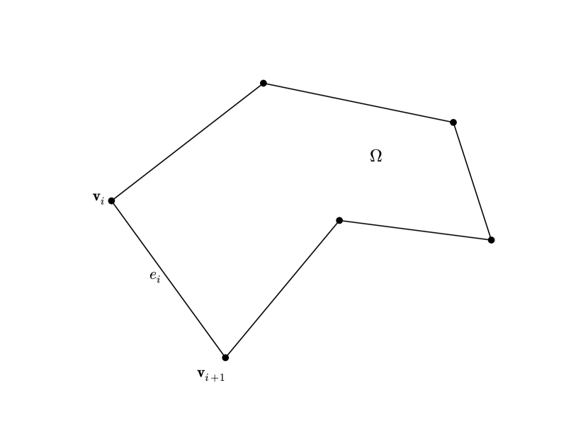
Figure 3: A simple (non-convex) polygon with vertices ${\mathbf{v}}_{i}$ and edges $e_{i}$.

4 Results

A series of test cases for plate bending and buckling is computed for different geometries. In section 4.1 bending and buckling of an annular plate is considered and compared to reference cases in the literature. The same is done for the geometry of a rectangular plate with and without holes in section 4.2. As an example of a more complicated shape, we consider bending and buckling of a polygonal plate with holes in section 4.3.

4.1 Annular plate

The geometry of the annular plate is sketched in figure 4. At the outer boundary with radius $b$ clamped boundary conditions are applied, whereas the inner boundary with radius $a$ is free. The weight function $\omega$, entering the definition of the basis functions, equation (41), is for this case defined by:

$$\omega(x,y)=\left(x^{2}+y^{2}-b^{2}\right)^{2}.$$ (56)

4.1.1 Bending of an annular plate by a lateral load

When considering plate bending for a constant lateral loading $p(x,y)=p_{0}$, an analytic solution can be found [3]:

$$w(r)=c_{1}\log(r)+c_{2}r^{2}\log(r)+c_{3}r^{2}+\frac{p_{0}}{64D}r^{4},$$ (57)

where $c_{1}$, $c_{2}$ and $c_{3}$ are functions of $a,b,\nu$ and $D$. Their exact definition is rather laborious but can easily be obtained by symbolic computation using the boundary conditions at the inner and outer boundary. Choosing $a=0.5345$, $b=1.5432$, $p_{0}=1.74586$, $\nu=0.3$ and $D=1.234$, we apply the present solver for different degrees $p$ and resolutions $h$ to the above problem. A surface plot of the solution is embedded in the convergence plot in figure 5, showing that the maximum deformation is obtained at the inner boundary and that the solution is axisymmetric. The present solver does, however, not employ the axisymmetry of the problem. It solves it on a rectangular Cartesian grid. In figure 5, we observe that the embedded boundary treatment of the weighted extended B-spline solver is indeed higher order accurate. For sufficiently small $h$,the error converges with the theoretical order of convergence for smooth problems, which is $p+1$.

Figure 4: Geometry of the annular plate with clamped outer boundary and free inner boundary. A constant lateral forcing is applied onto the plate.

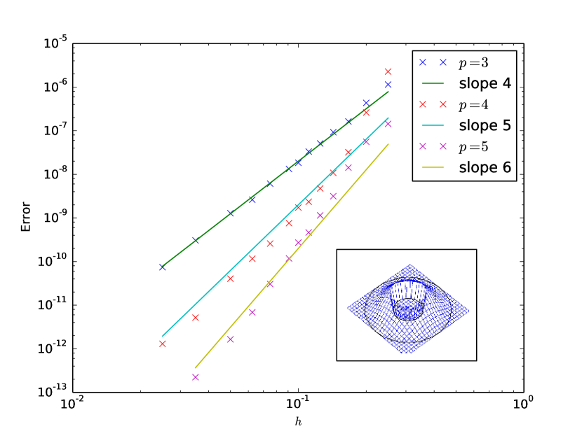
Figure 5: Convergence of the error of the numerical solution with respect to the cell size $h$ for the bending problem of an annular plate under constant lateral loading using splines of different degree $p$.

4.1.2 Buckling of an annular plate by in-plane loads

In this section, instead of a lateral loading, a radial compression force is applied at the outer boundary of an annular plate, cf. figure 6. The case of buckling of an annular plate has found some attention in the literature, cf. [42, 43, 44] and references therein. Concerning the choice of boundary conditions at the outer boundary, the more interesting case is for clamped boundary conditions. For this relatively simple geometry, the stress components of $\sigma$ can be found analytically and are given by [42]:

$$\sigma_{rr} = -\frac{1-a^{2}/r^{2}}{1-a^{2}/b^{2}}$$ (58)

$$\sigma_{\phi\phi} = -\frac{1+a^{2}/r^{2}}{1-a^{2}/b^{2}}$$ (59)

$$\sigma_{r\phi} = 0$$ (60)

in polar coordinates $(r,\phi)$. For the case $\nu=0.3$, the buckling stresses for the different modes have been plotted in figure 3 in [44]. These graphs have been digitized from figure 3 in [44] and are plotted together with the present results in figure 7. We solve equation (10) for five aspect ratios $a/b$, cases $(a)$ to $(e)$ in table 1, using the present weighted extended B-spline solver. The outer radius has been set to $b=2.28$. The critical stresses $\lambda_{c}$ from equation (10), are nondimensionalized by means of the $K$-value:

$$K=\frac{\lambda_{c}}{D/b^{2}},$$ (61)

and are reported in table 1 for two resolutions $h=0.2$ and $h=0.1$. As can be seen from the values found, approximately five significant digits are identical for both resolutions. The reference values have been read from figure 3 in [44]. The buckling modes corresponding to the cases in table 7 are plotted in figure 8. For increasing ratio $a/b$, the solution displays an increasing number of buckles in angular direction. From this relatively simple test case, we can conclude that the present solver based on an embedded description of the boundary provides accurate solutions for buckling problems.

Figure 6: Geometry of the annular plate with free inner boundary and clamped outer boundary. A constant in plane forcing in normal direction is applied onto the outer boundary.

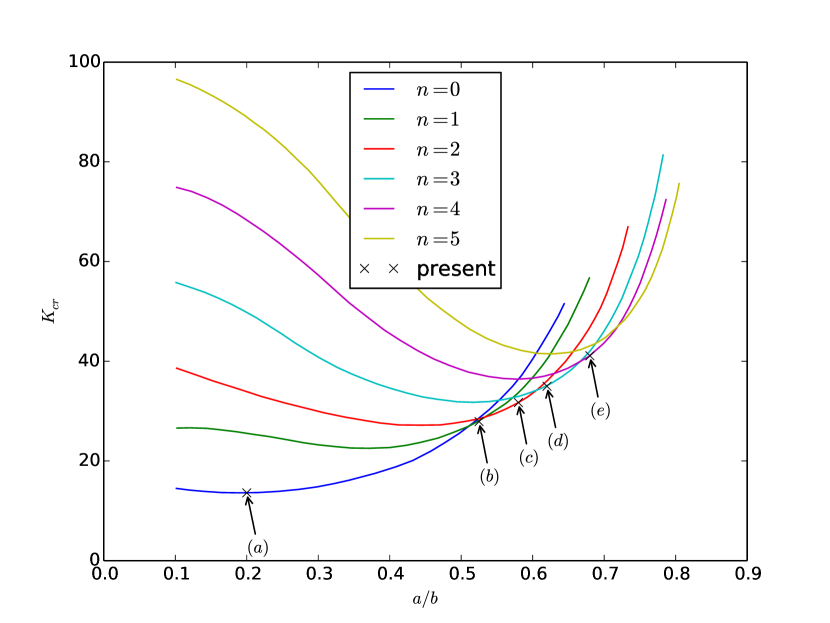
Figure 7: Critical buckling stresses for an annular plate with free inner and clamped outer boundary condition, as sketched in figure 6. The lines for the modes $n=0,\ldots 5$ are scanned form figure 3 in [44]. The buckling modes corresponding to the examples $(a),(b),(c),(d)$ and $(e)$ computed by means of the present method are plotted in figure 8.

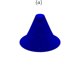
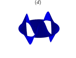
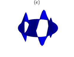
Figure 8: Buckling modes of an annular plate with free inner and clamped outer boundary condition for the cases denoted by $(a),(b),(c),(d)$ and $(e)$ in figure 7.

Table 1: K-values for the buckling of an annular plate for different ratios $a/b$ and resolutions $h$.

case	$a/b$	$K(h=0.2)$	$K(h=0.1)$	$K^{ref}$
(a)	0.2	13.60464726310300	13.60389138752100	13.6
(b)	0.525	27.90167587045000	27.90151625370600	28.0
(c)	0.58	31.71513802673000	31.71489313775400	31.7
(d)	0.62	34.99334267376700	34.99266753385800	35.1
(e)	0.68	41.10888319580700	41.10806291507800	41.1

4.2 Rectangular plate

For a rectangular plate defined by $[-a/2,a/2]\times[-b/2,b/2]$, the weight function in equation (41) is given for simply supported boundary conditions by

$$\omega(x,y)=\left(x+\frac{a}{2}\right)\left(\frac{a}{2}-x\right)\left(y+\frac{b}{2}\right)\left(\frac{b}{2}-y\right).$$ (62)

When dealing with clamped boundary conditions, we have to square the right hand side of (62). In section 4.2.1, where we rotate the plate with respect to the grid, the weight function (62) is rotated with the plate. In section 4.2.5, the pre-buckling stress in a plate with central hole is computed. For this case, we need in addition a simple weight for the boundary of the round hole:

$$\omega_{hole}(x,y)=x^{2}+y^{2}-\frac{d^{2}}{4},$$ (63)

where $d$ is the diameter of the hole.

4.2.1 Bending of a rectangular plate with aligned stiffener

A rectangular plate with side lengths $a$ and $b$ is supported by a stiffener located at the middle line parallel to the lower and upper boundary of the plate, cf. figure 9. In order to test the present embedded boundary description, we rotate the plate by an angle $\phi$ such that the geometry of the plate is no longer aligned with the grid. The plate is loaded by a constant loading $p_{0}$ and we use simply supported boundary conditions at the edges of the domain. The parameters of the simulation are given by:

$$a=5\quad b=1\quad D=1.234\quad EI=150\quad p_{0}=1.543.$$ (64)

The angle $\phi$ is set to $10^{\circ}$. For comparison, we perform a simulation with aligned geometry, meaning that we take $\phi=0^{\circ}$. A reference solution, computed on a fine grid, is used in order to compute the error of the numerical solution. In figure 10, the error of the solution is plotted in function of the cell size $h$ for splines of degree $p=3,5$. For the aligned case $\phi=0^{\circ}$, we observe that the convergence rate for the splines of degree $p=3$ is approximately four. However, for splines of degree $p=5$, we observe a smaller rate at approximately three. This can be explained by the jump condition (9) at the beam. As the third normal derivative of the solution is discontinuous, we expect a reduction of the convergence rate, since the third derivatives of the basis functions with degree $p=5$ are continuous. The third derivatives of the basis functions with $p=3$ are however not continuous at the grid lines and we therefore see the theoretical order of convergence, namely four. When rotating the domain by $10^{\circ}$, the stiffener is not aligned with the grid lines anymore and we observe a reduced convergence rate of approximately three for both degrees.

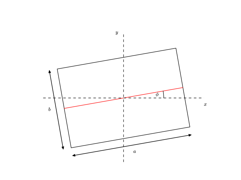
Figure 9: Geometry of a rectangular plate reinforced by a single stiffer (red color) parallel to the lower and upper boundary of the plate. The plate is rotated by an angle $\phi$ with respect to the coordinate axes $(x,y)$ defining the orientation of the computational cells. A uniform lateral loading is applied onto the plate.

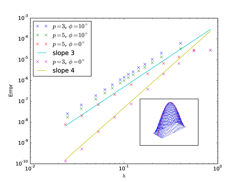
Figure 10: Convergence of the error of the numerical solution with respect to the cell size $h$ for the bending problem sketched in figure 9. The degree of the B-splines is given by $p=3,5$ and the inclination is either $\phi=0^{\circ}$ or $\phi=10^{\circ}$.

4.2.2 Buckling of a rectangular plate with aligned stiffener

This case corresponds to example 9.11 in [2]. As before, a simply supported plate is supported by a stiffener along its middle line. However, this time an in-plane force normal to the left and right boundary is applied, cf. figure 11. The stress field for this case is simply given by:

$$\sigma_{xx}=-1,\quad\sigma_{yy}=\sigma_{xy}=0.$$ (65)

The magnitude $T_{s}$ of the axial forcing for the stiffener, cf. equation (5), is given as in [2] by:

$$T_{s}=b\delta,\quad\delta=\frac{A}{bh},$$ (66)

where $A$ is the cross section area of the stiffener. Since the solution is symmetric around the stiffener, we have $\frac{\partial w}{\partial\zeta}=0$ on $\Gamma$, meaning that in the formula for the axial shortening (5) only the first term is nonzero. As in [2], we introduce the other nondimensional parameters controlling the system by:

$$\beta=\frac{a}{b}\quad\gamma=\frac{EI}{bD}.$$ (67)

The $K$-value for this system is defined as in [2]:

$$K=\frac{\lambda_{cr}b^{2}h}{\pi^{2}D}.$$ (68)

An analytic value for $K$ is given by the smaller root of equation (k) in example 9.11 in [2]. This value is plotted as a green line in figure 12 for the present choice of

$$\beta=\frac{5}{2}\quad\delta=\frac{1}{2}.$$ (69)

Formula (k) in [2], is, however, only valid in the case of the plate buckling into a single buckle. As can be observed from figure 12, for weak stiffeners, the buckled plate displays two buckles, whereas for strong stiffeners, only the plate displays buckling, whereas the stiffener stays straight, similar to what [45] (figure 6) have found before. For a single buckle the present method gives buckling stresses remarkably close to the approximate formula by [2].

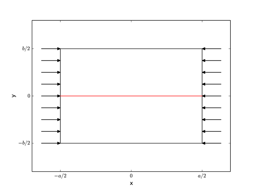
Figure 11: Geometry of a rectangular plate reinforced by a single stiffener (red color) parallel to the lower and upper boundary. Uniform in-plane loading is applied at the left and right boundaries.

Figure 12: Buckling of a rectangular plate reinforced by a single stiffener parallel to the lower and upper boundary of the plate with dimensions $a/b=5/2$ and aspect ratio between the cross section areas of the rip and the plate given by $A/(bh)=1/2$.

4.2.3 Bending of a square plate with non-aligned stiffener

In section 4.2.1, we observed that when the stiffener is no longer aligned with the grid lines, the rate of convergence is reduced due to the jump in the third derivative of the solution at the location of the beam. When faced with a stiffener crossing a simply supported square plate at a specific angle, cf. figure 13, we expect a reduction of the order of convergence. This can also be observed in the convergence plot, figure 14, for the present choice of parameters:

$$a=2\quad D=1.234\quad EI=150\quad p_{0}=1.543.$$ (70)

The order of convergence in figure 13 is, however, lower than anticipated from equation (9), i.e. two instead of three. The reason for this might lie in the development of a singularity at the intersections between stiffener and boundary of $\Omega$. A plot of the spatial distribution of the error for a specific resolution $h=0.02$, cf. figure 13, supports this possibility. Away from the beam the numerical solution seems to be close to the reference solution. Close to the beam we observe some smaller wiggles, whereas at the obtuse angles between boundary and stiffener, the error of the solution is largest. The appearance of singularities between stiffener and boundary reduces the accuracy of the method even if we had rotated the domain such that the stiffener would be aligned with one grid axis.

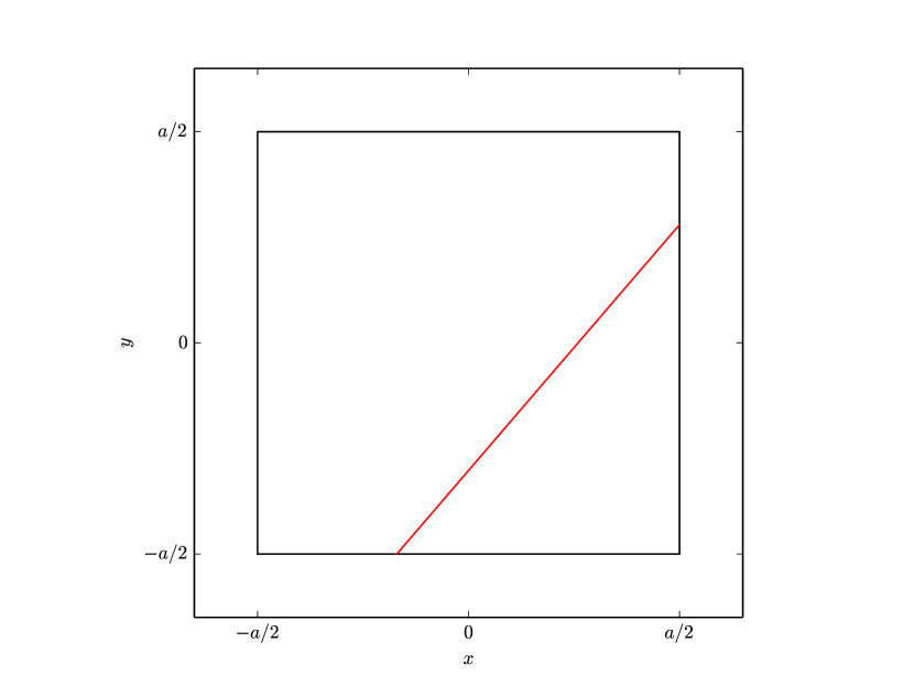
Figure 13: Geometry of a square plate reinforced by a single stiffer (red color) going from $(-0.17a,-a/2)$ to $(a/2,0.28a)$. A uniform lateral loading is applied onto the plate.

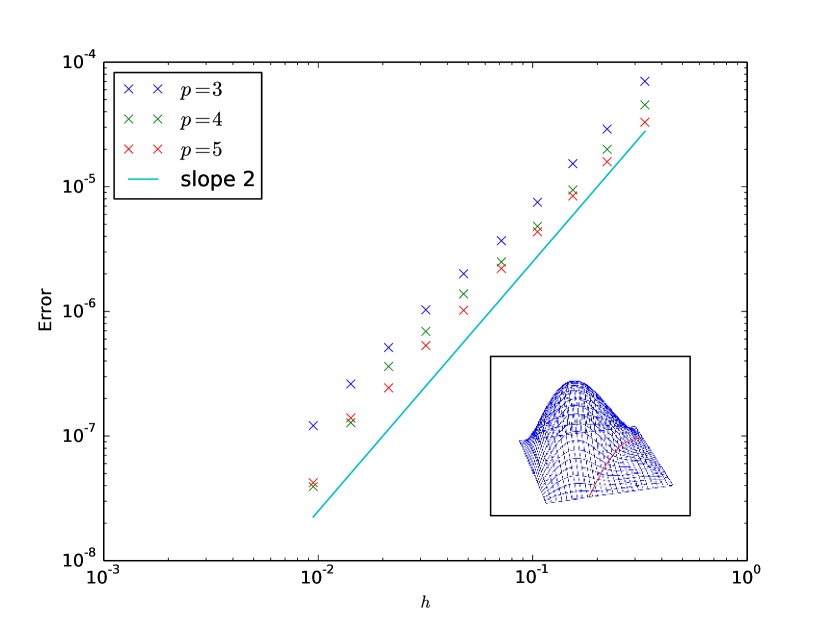
Figure 14: Convergence of the error of the numerical solution with respect to the cell size $h$ for the bending problem sketched in figure 13. The degree of the B-splines is given by $p=3,4,5$.

Figure 15: Absolute difference between the solution $w$ for $p=3$ and $h=0.02$ and the reference solution $w^{ref}$ ($p=3$ and $h=0.005$) for the problem sketched in figure 13.

4.2.4 Buckling of a square plate with non-aligned stiffener

Instead of a lateral loading, an in-plane loading can be applied to the left and right boundaries of the domain, cf. figure 16. Assuming that no axial forcing is applied onto the stiffener, $T_{s}=0$, we solve (10) for a simply supported and clamped square plate for different values of $EI/(Db)$. As can be observed from figure 17, the buckling stress is a smooth function of the stiffness ratio. For large ratios, the stiffener is almost flat, whereas for $EI=0$, we obtain the reference $K$ values for simply supported and clamped plates, i.e. $4$ and $9.4$, respectively.

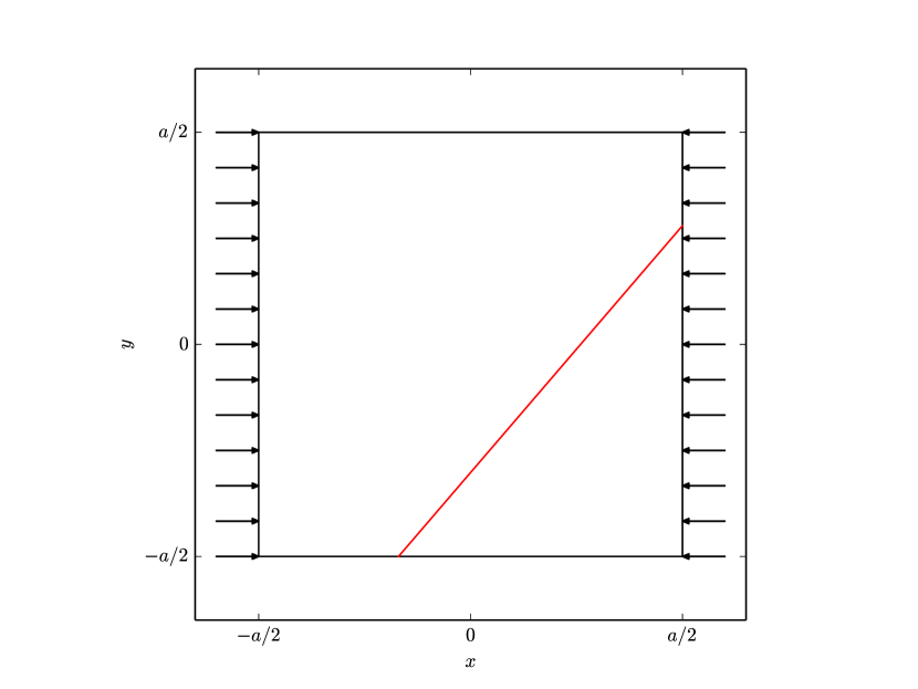
Figure 16: Geometry of a square plate reinforced by a single stiffer (red color) going from $(-0.17a,-a/2)$ to $(a/2,0.28a)$. A uniform in plane lateral loading is applied at the right and left boundary.

Figure 17: Buckling of a square plate reinforced by a single stiffener (red color) going from $(-0.17a,-a/2)$ to $(a/2,0.28a)$ for simply supported and clamped boundary conditions.

4.2.5 Pre-buckling stress of a rectangular plate with central hole

In the following, we add a hole in the center of the rectangular plate, cf. figure 18. When considering buckling, we are faced with the difficulty that no analytic formula is known for the pre-buckling stress for a rectangular plate with a central hole with free boundary conditions. Therefore, the pre-buckling stress will be computed numerically by the approach presented in section 3.2. In a first attempt, we shall verify the present method by applying it to the case when uniform normal compression is applied both at the outer boundary and at the hole, cf. figure 18. For this configuration, the reference solution is given by

$$\sigma_{xx}=\sigma_{yy}=-1\quad\sigma_{xy}=0.$$ (71)

For a plate with parameters

$$a=4\quad b=2\quad d=1,$$ (72)

where $d$ is the diameter of the hole, the error of the numerical solution in function of $h$ for splines of degree $3$ and $5$ is plotted in figure 19. Since the error is measured on the stress components which are given by the second derivatives of Airy’s stress function, the order of convergence is reduced by approximately two.

For the case of a uniform tension force on the right and left boundary and a free boundary at the upper and lower edges and at the hole, cf. figure 20, a reference solution is given in figure 1 in [46]. Applying the present method to the case treated in [46], we can compare the values of $\sigma_{xx}$ and $\sigma_{yy}$ along the $x$-axis found by the present method with the values obtained in [46], cf. figure 21. The present numerical solution has been obtained by means of splines of degree 3. For the relatively coarse resolution of $h=0.5$, i.e six cells, along the $x$-axis in figure 21, we observe kinks in the solution due to the fact that the third derivative of the basis functions for $p=3$ is in general discontinuous at the cell boundaries. These kinks are no longer visible for the finer resolutions $h=0.1,0.05$, when the solution is indistinguishable on a plotting scale. When choosing $p=5$, the solution is smooth even for coarse resolutions (figure not shown). In general the lines follow the solution by [46] closely. The discrepancy might be associated to the modest plotting quality of figure 1 in [46], which is passed further to the digitized data. As the stress components enter the buckling energy (3), it is advantageous to use B-splines of degree $p+2$ for Airy’s stress function, when B-splines of degree $p$ are used for the vertical displacement $w$.

Figure 18: Geometry of a rectangular plate $[-a/2,a/2]\times[-b/2,b/2]$ with central hole with diameter $d$. A uniform in-plane compression force is applied in normal direction to the boundaries, such that the resulting stress tensor is given by $\sigma_{xx}=\sigma_{yy}=-1$ and $\sigma_{xy}=0$.

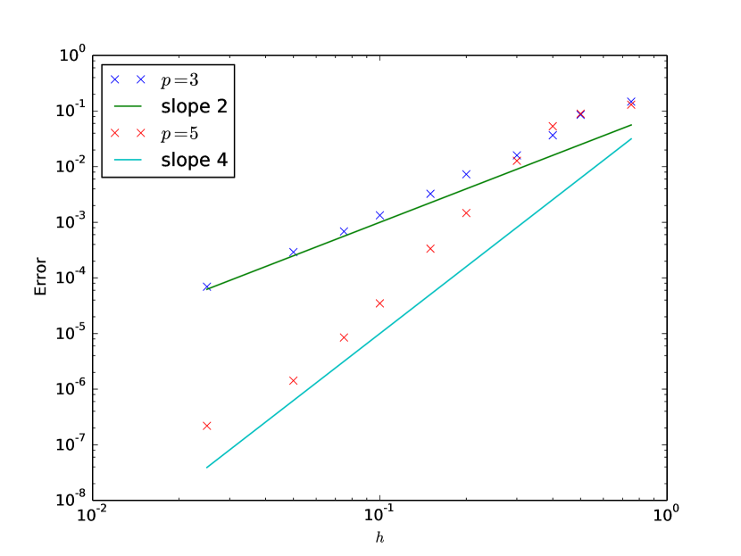
Figure 19: Error convergence of the pre-buckling stress problem sketched in figure 18. Since the error is measured on the stress components which are given by the second derivatives of Airy’s stress function, the order of convergence is reduced by two.

Figure 20: Geometry of a rectangular plate $[-a/2,a/2]\times[-b/2,b/2]$ with central hole with diameter $d$. A uniform in-plane tension force is applied on the right and left boundaries. The set-up corresponds to the plane stress problem solved in [46].

Figure 21: Stress along the positive part of the $x$ axis for the problem sketched in figure 20. The numerical results for $p=3$ and different choices of $h$ are compared to the results obtained by [46]. The data for Hayashi has been digitized form figure 1 in [46]. The lines for $h=0.1$ and $h=0.05$ are indistinguishable on a plotting scale.

4.2.6 Buckling of a square plate with central hole

This case has been solved in several works, for example [47, 14, 16]. A square plate with a free hole in its center is uniformly loaded in-plane at its left and right boundary, cf. figure 22. The pre-buckling stress field has been computed by means of the method in section 3.2. This stress field is then used to solve the buckling problem (10) by the present method with splines of degree $p=3$, a resolution of $h=0.025,0.05,0.1$, a side length of $a=2$, and for a Poisson module of $\nu=0.3$. The $K$ values of the buckling stress computed by the present method are compared to the results obtained by Zhong et al.[14] in figure 23. The results by Zhong et al. were digitized from figure 13 in [14]. The present results lie neatly on top of the graph by the data obtained by [14]. In addition, we checked that, apart from the smallest hole for $h=0.1$, the present results are indistinguishable on a plotting scale for $h=0.025,0.05,0.1$.

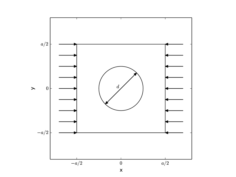
Figure 22: Geometry of a square plate with central hole. A uniform in-plane loading is applied onto the left and right boundaries.

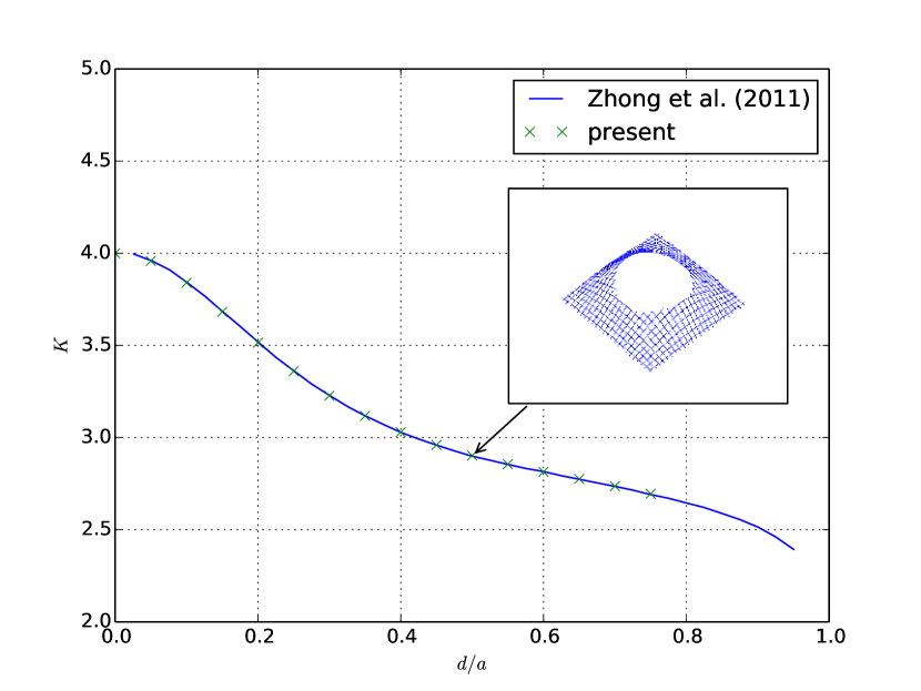
Figure 23: Buckling stress for a square plate with central hole in function of the ratio between hole diameter $d$ and plate dimension $a$. The data for Zhong et al. has been digitized from figure 13 in [14]. The embedded figure shows the eigenfunction for the case $d/a=0.5$.

4.3 Polygonal plate

In this section we turn to our last test, where we employ the present solver on a more general domain. We consider two cases, a plate with holes bounded by a convex polygon and a plate with holes bounded by a simple, non convex polygon, cf. figures 24 and 25. We shall first consider bending, cf. section 4.3.1, before turning our attention to buckling, cf. section 4.3.2. As before, a definition for the weight function in equation (41) needs to be given for the present domains. For the geometry bounded by a convex polygon, a weight function can be written as:

$$\omega(x,y)=\left(\prod\limits_{i=0}^{4}\omega_{i}(x,y)\right)^{2},$$ (73)

where $\omega_{i}$ is defined in equation (93). The right hand side in (73) is squared in order to model clamped boundary conditions. For the external boundary of the non-convex polygon, on the other hand, a simple product of the edge weights $\omega_{i}$ as in (73) cannot be used. For the inward facing corner at ${\mathbf{v}}_{0}$, set operations as for the R-function method [48] need to be used in order to define a weight function. The resulting weight function is in this case given by:

$$\omega(x,y)=\left(\omega_{{c}}\prod\limits_{i=1}^{3}\omega_{i}(x,y)\right)^{2},$$ (74)

where

$$\omega_{{c}}=\omega_{0}+\omega_{4}+\sqrt{\omega_{0}^{2}+\omega_{4}^{2}}.$$ (75)

For the computation of the stress field for the buckling problem, we need in addition a simple weight for the holes in the domain. The weight

$$\omega_{{hole}}=\left(x-x_{0}\right)^{2}+\left(y-y_{0}\right)^{2}-R^{2}$$ (76)

is used for a circular hole of radius $R$ centered at $(x_{0},y_{0})$. The coordinates of the vertices of the bounding polygons and the position and radius of the holes can be found in B.

4.3.1 Bending of a polygonal plate with holes

In the present section, a constant lateral loading $p_{0}$ is applied onto the plates defined in figures 24 and 25. The parameters of the simulation are given by:

$$p_{0}=1.234,\quad D=1,\quad\nu=0.3.$$ (77)

By using a numerical solution on a fine grid as reference solution, a numerical error can be computed. As can be seen from figure 26, the theoretical convergence rates for the solver are approximately recovered for the domain with convex outer boundary. However, when applying the method to the domain displaying an inward facing corner at ${\mathbf{v}}_{0}$, cf. figure 25, the rate of convergence drops to a value of approximately two, cf. figure 27. The reason for this is the development of a singularity at the external corner reducing the convergence rate of the method, cf. [49].

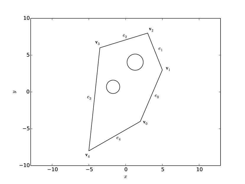
Figure 24: Geometry of a plate with holes bounded by a convex polygon. A uniform lateral loading is applied onto the plate.

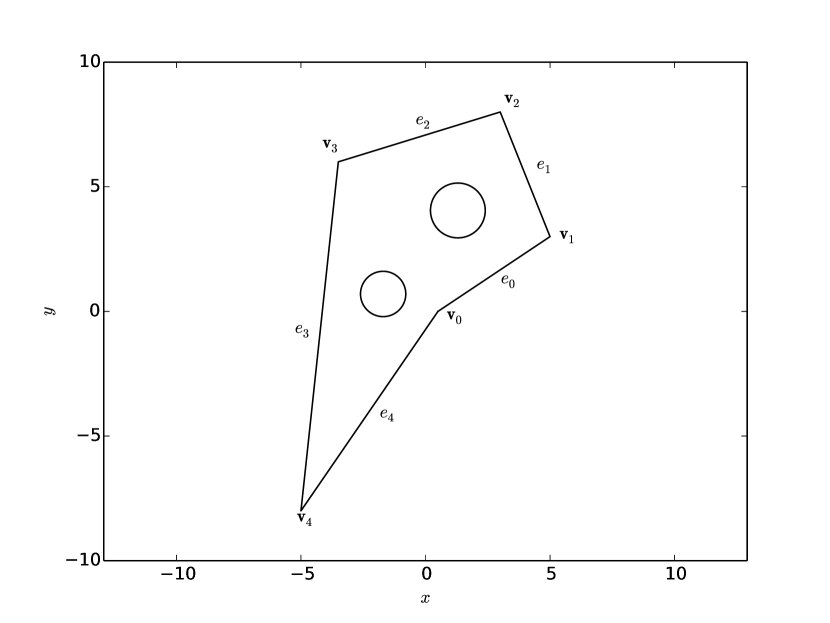
Figure 25: Geometry of a plate with holes bounded by a non convex polygon. A uniform lateral loading is applied onto the plate.

Figure 26: Error convergence of the bending problem sketched in figure 24.

Figure 27: Error convergence of the bending problem sketched in figure 25.

4.3.2 Buckling of a polygonal plate with holes

A simple buckling problem for the present plates with holes bounded by a polygon, can be defined by applying a normal compression onto the exterior boundary, cf. figures 28 and 29. In table 2, the buckling stresses $\lambda_{c}$ are recorded for the two geometries for two resolutions $h$ using splines of degree $3$. As can be observed, for the convex polygon, four digits of the buckling stress have been obtained, whereas for the non-convex polygon, three digits have been reached. The eigenfunctions corresponding to the buckling stress are plotted in figures 30 and 31.

Table 2: Buckling of a polygonal plate with holes.

$h$	$\lambda_{c}/D$
Convex polygon
0.3	0.578828
0.15	0.578869
Non convex polygon
0.3	0.851154
0.15	0.851590

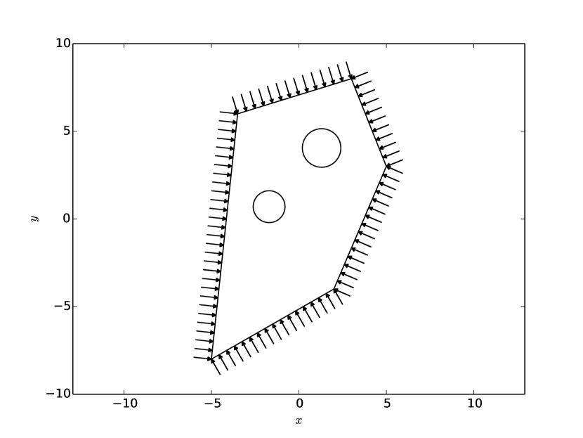
Figure 28: Geometry of a plate with holes bounded by a convex polygon. A uniform in-plane loading in-normal direction applied onto the edges of the outer boundary. The holes are free.

Figure 29: Geometry of a plate with holes bounded by a non convex polygon. A uniform in-plane loading in-normal direction applied onto the edges of the outer boundary. The holes are free.

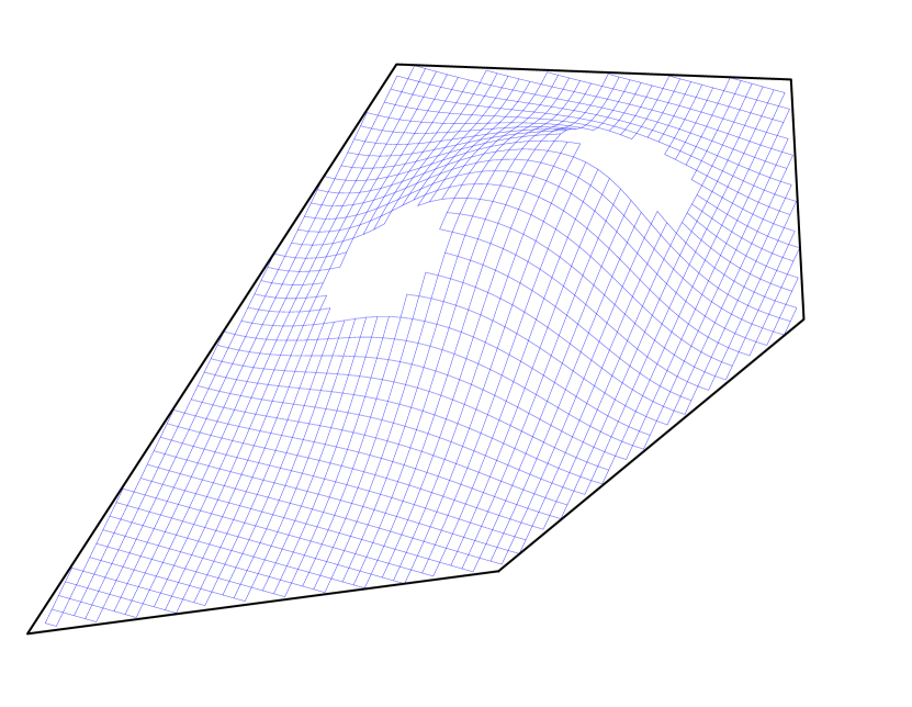
Figure 30: Most unstable buckling eigenmode for the plate with holes bounded by a convex polygon, cf. figure 28.

Figure 31: Most unstable buckling eigenmode for the plate with holes bounded by a non convex polygon, cf. figure 29.

5 Conclusions

In the present treatise, the weighted extended B-spline method by [30] is applied to bending and buckling problems of Kirchhoff plates of various shapes for lateral and in-plane loading. The plate is allowed to be supported by a stiffener. A range of benchmark tests is applied to the present solver in order to document various aspects affecting the accuracy of the present method. In particular, we document how the jump conditions at the stiffener location and singularities at the intersection between stiffener and boundary of the domain or at inward facing corners reduce the accuracy of the method. However, for smooth solutions, the present method displays high order accuracy, making it a formidable choice for eigenvalue problems, such as plate buckling problems, due to the relatively small size of the stiffness matrix.

As such, techniques have been developed for the treatment of singularities and discontinuities in the framework of other methods [50, 49, 51, 31, 52]. However, it remains to future research how exactly these can be applied to the weighted extended B-spline method in order to recover the higher accuracy. As is pointed out in the present work and also in [9], singularities have a bigger impact on the accuracy than the reduced continuity at the stiffener location and should therefore be addressed first.

Concerning the computational efficiency of the present method, the cost of the assembly of the matrices depends heavily on the complexity of the domain. In general, the cost scales approximately linearly with the number of cells, i.e. $\propto h^{-2}$. The sparse linear solver by Tim Davis [37] leads to a scaling of approximately $\propto h^{-4}$ for the solution of the bending problem (42). Concerning the eigenvalue solver, the sparsity is not taken into account by using a Lapack solver [38] for full matrices, i.e. the computational cost scales as $\propto h^{-6}$. The application of an iterative eigenvalue solver would have reduced this cost significantly.

A difficulty observed in the present work for the weighted extended B-spline method is the treatment of small holes as in section 4.2.6. As the smallest features of the geometry dictate the resolution $h$, small cells are used also in regions of the domain where a coarser resolution would have been enough. In section 4.5 in [30], ideas for the formulation of a weighted extended B-spline method using hierarchical bases are presented. Such a development allowing to use different resolutions for parts of the domain would be a very welcome feature for the method.

The embedded treatment of the boundary of the domain is an interesting feature in order to facilitate the integration between CAD and structural solver. However, it is also Achilles’ heel of the method, as the cost of the assembly of the system is dominating. We remark that the present code might not have been fully optimized with respect to this point and that a better balancing of the approximation error would give some improvement. On the other hand, a collocation formulation of the weighted extended B-spline method as in [53] would render this issue obsolete.

The aim of the present treatise is to give an account of the weighted extended B-spline method when applied to plate bending and buckling problems relevant for the maritime industry. We highlight a number of issues which are important when considering bending and buckling of plates. Although the accuracy of the method is affected by these issues (which holds true also for other methods), it nevertheless is a remarkably accurate method applicable to a wide range of problems.

6 Acknowledgments

The author would like to thank Dr Eivind Steen and Dr Lars Brubak for the many interesting, helpful and motivating meetings at DNV-GL. Professor Jostein Hellesland and Professor Brain Hayman are thanked for interesting discussions. Professor Michael Floater is heartily thanked for his patience checking the extension algorithm.

Appendix A Extension algorithm for weighted extended B-Splines

Poisson problem

We start with the Poisson case, meaning that boundary data is only given for the function values. The biharmonic case will be treated below. The aim is to find a function $\tilde{u}$ defined in $\Omega$ sufficiently smooth, such that $\tilde{u}$ satisfies the boundary data:

$$\tilde{u}=f\quad\mbox{on}\quad\partial\Omega\\$$ (78)

As sketched in figures 3 and 32, the boundary of the domain $\Omega$ consists of an $n$ sided simple polygon. Each edge $e_{i}$ is connected by adjacent vertices $\mathbf{v}_{i}$ and $\mathbf{v}_{i+1}$ with components

$${\mathbf{v}}_{i}=\left({u_{i}\atop v_{i}}\right).$$ (79)

We assume that none of the vertices ${\mathbf{v}}_{i}$ is degenerated. Each edge $e_{i}$ defines a coordinate transformation ${\mathbf{x}}_{i}(\alpha,\beta)$ by:

$${\mathbf{x}}_{i}(\alpha,\beta) = \left(\begin{array}[]{c}x_{i}(\alpha,\beta)\\ y_{i}(\alpha,\beta)\end{array}\right)$$ (82)

$$= {\mathbf{v}}_{i}+{\mathbf{t}}_{i}\alpha+{\mathbf{n}}_{i}\beta$$ (83)

$$= \left({u_{i}\atop v_{i}}\right)+\left({t_{x}^{i}\atop t_{y}^{i}}\right)\alpha+\left({n_{x}^{i}\atop n_{y}^{i}}\right)\beta,$$ (84)

where ${\mathbf{t}}_{i}$ and ${\mathbf{n}}_{i}$ are the tangential and normal vectors of the edge $e_{i}$:

$${\mathbf{t}}_{i} = \frac{1}{L_{i}}\left({{u_{i+1}-u_{i}}\atop{v_{i+1}-v_{i}}}\right),$$ (85)

$${\mathbf{n}}_{i} = \left({t^{i}_{y}\atop-t_{x}^{i}}\right),$$ (86)

$$L_{i} = \sqrt{(u_{i+1}-u_{i})^{2}+(v_{i+1}-v_{i})^{2}}.$$ (87)

For the components of the tangential and normal vector, the index denoting the edge is written as a superscript in order to simplify the notation. The inverse transformation of ${\mathbf{x}}_{i}$ is given by

$$\boldsymbol{\alpha}_{i}(x,y) = \left({\alpha_{i}(x,y)\atop\beta_{i}(x,y)}\right)$$ (88)

$$= \left(\begin{array}[]{cc}t_{x}^{i}&t_{y}^{i}\\ t_{y}^{i}&-t_{x}^{i}\end{array}\right)\left({{x-u_{i}}\atop{y-v_{i}}}\right).$$ (91)

Each edge is parametrized by the arclength $s$ going from $0$ to $L_{i}$, the total arclength of the edge. Thus for any point $(x,y)$ on the edge $e_{i}$, we have:

$$\alpha_{i}(x,y)=s\in[0,L_{i}]\quad\mbox{and}\quad\beta_{i}(x,y)=0,\quad(x,y)\in e_{i}.$$ (92)

We assume in addition, that each edge $e_{i}$ can be extended by an amount $\Delta s_{i}$, such that the extended edge $\tilde{e}_{i}$ controlled by the parameter $s\in[-\Delta s_{i},L_{i}+\Delta s_{i}]$ has, as $e_{i}$, only two intersections with the other edges, namely $\mathbf{v}_{i}$ and $\mathbf{v}_{i+1}$, cf. the dashed line in figure 32.

Since ${\mathbf{n}}_{i}$ is pointing outward of the domain, we can define a weight $\omega_{i}(x,y)$ for each edge by

$$\omega_{i}(x,y)=-\beta_{i}(x,y).$$ (93)

For a convex polygon $\omega_{i}(x,y)$ would be positive in the interior. We note

$$\Omega_{i}(x,y)=\omega_{i-1}(x,y)\omega_{i+1}(x,y),$$ (94)

which is zero at the edges $e_{i-1}$ and $e_{i+1}$ and nonzero at $e_{i}$ for $s\in]0,L_{i}[$, and has simple roots at $s=0$ and $s=L_{i}$. For each vertex $\mathbf{v}_{i}$ we define a radial hat function $h_{i}(\mathbf{x})$ given by:

$$h_{i}(\mathbf{x})=\exp-\frac{|\mathbf{x}-\mathbf{v}_{i}|^{2}}{R_{i}^{2}},$$ (95)

which is a Gaussian with variance $R_{i}$. Finally, the boundary data $f$ in equation (78) is given by a function $f_{i}(s)$ for each edge $e_{i}$. We assume that the boundary data is compatible at the vertices, in the sense that

$$f_{i}(L_{i})=f_{i+1}(0).$$ (96)

The extension function $\tilde{u}$ in the Poisson case, equation (78), is then written as:

$$\tilde{u}(x,y)=\sum\limits_{i=1}^{n}a_{i}h_{i}(x,y)+\sum\limits_{i=1}^{n}\phi_{i}(\alpha_{i}(x,y))\Omega_{i}(x,y)r^{p+1}_{i}(\beta_{i}(x,y)),$$ (97)

where $r_{i}$ is a shape function defined by

$$r_{i}(x)=\left\{\begin{array}[]{ll}\frac{(D_{i}-x)(x+D_{i})}{D_{i}^{2}}&-D_{i}\leq x\leq D_{i}\\ 0&\mbox{otherwise}\end{array}\right.$$ (98)

The length $D_{i}$ must be chosen such that the quadrilateral defined by the vertices:

$${\mathbf{x}}_{i}(-\Delta s_{i},-D_{i}),\,{\mathbf{x}}_{i}(-\Delta s_{i},D_{i}),\,{\mathbf{x}}_{i}(L_{i}+\Delta s_{i},D_{i}),\,{\mathbf{x}}_{i}(L_{i}+\Delta s_{i},-D_{i})$$ (99)

does only have intersections with the edges $e_{i-1}$ and $e_{i+1}$. We remark that the function $r^{p+1}_{i}(\beta_{i}(x,y))$ is of class $\mathcal{C}^{p}$ in $\Omega$. The coefficients $a_{i}$ and functions $\phi_{i}(s)$ are unknown a priori, but we require that $\phi_{i}$ vanishes outside the interval $[-\Delta s_{i},L_{i}+\Delta s_{i}]$:

$$\phi_{i}(s)=0\quad\mbox{for}\quad s<-\Delta s_{i}\quad\mbox{and}\quad s>L_{i}+\Delta s_{i}.$$ (100)

In figure 32, we plotted the extended edge $\tilde{e}_{i}$ by a dashed line. On this line we marked the end points of $\tilde{e}_{i}$, i.e. ${\mathbf{x}}_{i}(-\Delta s_{i},0)$ and ${\mathbf{x}}_{i}(L_{i}+\Delta s_{i},0)$, by means of the mapping ${\mathbf{x}}_{i}$, equation (84), defined by the edge $e_{i}$. The points ${\mathbf{x}}_{i}(0,0)$ and ${\mathbf{x}}_{i}(L_{i},0)$ return the vertices ${\mathbf{v}}_{i}$ and ${\mathbf{v}}_{i+1}$, respectively. Due to the finite support of $\phi_{i}$ and $r_{i}$, the $i^{th}$ term in the second sum of equation (97) has a finite support given by the dotted box in figure 32 with corners given in equation (99).

In order to determine the coefficients $a_{i}$, we evaluate $\tilde{u}$ at the vertices ${\mathbf{v}}_{j}$:

$$\tilde{u}({\mathbf{v}}_{j})=\sum\limits_{i=1}^{n}a_{i}h_{i}({\mathbf{v}}_{j}),\quad j=1,\ldots,n,$$ (101)

since the second sum in (97) vanishes at the vertices. The function value $\tilde{u}({\mathbf{v}}_{j})$ must equal $f_{j}(0)$ by definition, which gives us a system of $n$ equations for the $n$ unknown $a_{i}$. In order to determine the unknown functions $\phi_{i}$, we evaluate $\tilde{u}$ at a point $(x,y)$ on the edge $e_{j}$:

$$\tilde{u}(x,y)=\sum\limits_{i=1}^{n}a_{i}h_{i}(x,y)+\phi_{j}(\alpha_{j}(x,y))\Omega_{j}(x,y).$$ (102)

A first choice $\tilde{\phi}_{j}(s)$ for $\phi_{j}(s)$ would be

$$\tilde{\phi}_{j}(s)=\frac{f_{j}(s)-\sum\limits_{i=1}^{n}a_{i}h_{i}(x_{j}(s,0),y_{j}(s,0))}{\Omega_{j}(x_{j}(s,0),y_{j}(s,0))},$$ (103)

which is well defined for $s=0$ and $s=L_{i}$, since the numerator goes equally fast (or faster) to zero as the denominator. If the boundary data $f_{j}$ is of class $\mathcal{C}^{p}([0,L_{i}])$, so is $\tilde{\phi}_{j}$. However, the behavior of $\tilde{\phi}_{j}$ outside of the interval $[0,L_{i}]$ is not controlled. We shall therefore choose a function $\phi_{j}(s)$ which is sufficiently smooth on the entire $\mathbb{R}$ axis and vanishes outside of the interval $[-\Delta s_{i},L_{i}+\Delta s_{i}]$. This function $\phi_{j}(s)$ can, however, only be an approximation to $\tilde{\phi}_{j}$. The extension $\tilde{u}$ will therefore not be an exact extension but only an approximate extension, which is, however, not a problem, as long as the approximation is sufficiently close in order not to reduce the accuracy of the overall solution. We use a spline interpolation of degree $p+1$ for $\phi_{j}$, where we assume that $p$ is even for simplicity. For each edge $e_{j}$, we choose a number $N_{j}$ and define a sequence of knots $\xi_{k}$ with:

$$\xi_{-(p+1)}=-\Delta s_{j},\quad\xi_{0}=0,\quad\xi_{N_{j}}=L_{j},\quad\xi_{N_{j}+(p+1)}=L_{j}+\Delta s_{j}.$$ (104)

The position of the other knots may be chosen arbitrarily as long as the sequence $\xi_{k}$ is monotonically increasing. In the present treatise, we choose a uniform distribution of knots $\xi_{k}$. The interpolant $\phi_{j}$ is thus a linear combination of $N_{j}+p+1$ B-splines:

$$\phi_{j}=\sum\limits_{k=-{p+1}}^{N_{j}-1}c_{k}b_{k}^{p+1}(s).$$ (105)

The $N_{j}+p+1$ conditions allowing to determine the $c_{k}$ are given by

$$\phi_{j}(\xi_{k}) = \tilde{\phi}_{j}(\xi_{k}),\quad k=0,\dots,N_{j}$$ (106)

$$\frac{d^{q}}{ds^{q}}\phi_{j}(\xi_{0}) = \frac{d^{q}}{ds^{q}}\tilde{\phi}_{j}(\xi_{0}),\quad q=1,\ldots,p/2$$ (107)

$$\frac{d^{q}}{ds^{q}}\phi_{j}(\xi_{N}) = \frac{d^{q}}{ds^{q}}\tilde{\phi}_{j}(\xi_{N}),\quad q=1,\ldots,p/2$$ (108)

Finally, the extension $\tilde{u}$ defined by the above procedure will be of class $\mathcal{C}^{p}$ inside the polygon $\Omega$ and on the boundary $\partial\Omega$ if the boundary data is sufficiently smooth.

The biharmonic case is more involved. In this case not only the function value is imposed on the boundary, but also its normal derivative:

$$\tilde{u} = f\quad\mbox{on}\quad\partial\Omega$$ (109)

$$\frac{\partial}{\partial n}\tilde{u} = g\quad\mbox{on}\quad\partial\Omega$$ (110)

In addition to an $f_{i}$ for each edge, we are given a function $g_{i}$ matching the normal derivative of $\tilde{u}$ at $e_{i}$. Next to the compatibility condition (96), constraints on the first and second derivative arise. For the first derivative we can write:

$$\left({\frac{d}{ds}f_{i}(L_{i})\atop\frac{d}{ds}f_{i+1}(0)}\right) = \left(\begin{array}[]{cc}t_{x}^{i}&t_{y}^{i}\\ t^{i+1}_{x}&t_{y}^{i+1}\end{array}\right)\left({\frac{\partial}{\partial x}\tilde{u}({\mathbf{v}}_{i+1})\atop\frac{\partial}{\partial y}\tilde{u}({\mathbf{v}}_{i+1})}\right)$$ (113)

$$\left({g_{i}(L_{i})\atop g_{i+1}(0)}\right) = \left(\begin{array}[]{cc}n_{x}^{i}&n_{y}^{i}\\ n^{i+1}_{x}&n_{y}^{i+1}\end{array}\right)\left({\frac{\partial}{\partial x}\tilde{u}({\mathbf{v}}_{i+1})\atop\frac{\partial}{\partial y}\tilde{u}({\mathbf{v}}_{i+1})}\right)$$ (116)

Inverting (113) and (116) leads to two additional compatibility conditions to be fulfilled by $f$ and $g$:

$$t_{y}^{i+1}\frac{d}{ds}f_{i}(L_{i})-t_{y}^{i}\frac{d}{ds}f_{i+1}(0) = -t_{x}^{i+1}g_{i}(L_{i})+t_{x}^{i}g_{i+1}(0)$$ (117)

$$-t_{x}^{i+1}\frac{d}{ds}f_{i}(L_{i})+t_{x}^{i}\frac{d}{ds}f_{i+1}(0) = -t_{y}^{i+1}g_{i}(L_{i})+t_{y}^{i}g_{i+1}(0)$$ (118)

A fourth compatibility condition arises from the fact that four derivatives are imposed at ${\mathbf{v}}_{i+1}$, namely

$$\frac{d^{2}}{ds^{2}}f_{i}(L_{i}),\quad\frac{d^{2}}{ds^{2}}f_{i+1}(0),\quad\frac{d}{ds}g_{i}(L_{i}),\quad\frac{d}{ds}g_{i+1}(0),$$ (119)

but only three unknowns are available, which are

$$\frac{\partial^{2}}{\partial x^{2}}\tilde{u}({\mathbf{v}}_{i+1}),\quad\frac{\partial^{2}}{\partial y^{2}}\tilde{u}({\mathbf{v}}_{i+1}),\quad\mbox{and}\quad\frac{\partial^{2}}{\partial x\partial y}\tilde{u}({\mathbf{v}}_{i+1}).$$ (120)

After some algebra the compatibility equation can be obtained as:

$${\mathbf{t}}_{i}\cdot{\mathbf{n}}_{i+1}\left(\frac{d^{2}}{ds^{2}}f_{i}(L_{i})+\frac{d^{2}}{ds^{2}}f_{i+1}(0)\right)+{\mathbf{t}}_{i}\cdot{\mathbf{t}}_{i+1}\left(-\frac{d}{ds}g_{i}(L_{i})+\frac{d}{ds}g_{i+1}(0)\right)=0$$ (121)

Given compatible $f$ and $g$, we shall, as for the Poisson case, consider the vertices first, before turning to the edges. However, for the biharmonic case, we need to impose in addition to the function value $\tilde{u}$, the first and second order derivatives of $\tilde{u}$ at the vertices. This is done by choosing the following expansion for $\tilde{u}$:

$$\tilde{u} = \sum\limits_{i=1}^{n}H_{i}(x,y)$$ (122)

$$+ \sum\limits_{i=1}^{n}\phi_{i}(\alpha_{i}(x,y))\Omega_{i}^{3}(x,y)r_{i}^{p+1}\left(\beta_{i}(x,y)\right)$$

$$+ \sum\limits_{i=1}^{n}\psi_{i}(\alpha_{i}(x,y))\Omega_{i}^{2}(x,y)\omega_{i}(x,y)r_{i}^{p+1}\left(\beta_{i}(x,y)\right)$$

where the function $H_{i}(x,y)$ collects all the coefficients for the conditions on the vertices:

$$H_{i}=a_{i}h_{i}+b_{i}\omega_{i}h_{i}+c_{i}\omega_{i+1}h_{i}+d_{i}\omega_{i}^{2}h_{i}+e_{i}\omega_{i+1}^{2}h_{i}+k_{i}\omega_{i}\omega_{i+1}h_{i}.$$ (123)

The weighting of $\phi_{i}$ and $\psi_{i}$ by $\Omega_{i}^{3}$ and $\Omega_{i}^{2}\omega_{i}$, respectively, is such that for derivatives up to the third order the second and third sum in equation (122) vanish at the vertices. For this reason the 6 coefficients, $a_{i}$, $b_{i}$, $c_{i}$, $d_{i}$, $e_{i}$, and $k_{i}$ in $H_{i}$, can be determined by 6 conditions at the vertices ${\mathbf{v}}_{j}$, $j=1,\ldots,n$:

$$\sum\limits_{i=1}^{n}H_{i}({\mathbf{v}}_{j}) = f_{j}(0)$$ (124)

$$\sum\limits_{i=1}^{n}{\mathbf{t}}_{j}\cdot\nabla H_{i}({\mathbf{v}}_{j}) = \frac{d}{ds}f_{j}(0)$$ (125)

$$\sum\limits_{i=1}^{n}{\mathbf{n}}_{j}\cdot\nabla H_{i}({\mathbf{v}}_{j}) = g_{j}(0)$$ (126)

$$\sum\limits_{i=1}^{n}{\mathbf{t}}_{j}\cdot\left(\nabla\nabla H_{i}({\mathbf{v}}_{j})\right)\cdot{\mathbf{t}}_{j} = \frac{d^{2}}{ds^{2}}f_{j}(0)$$ (127)

$$\sum\limits_{i=1}^{n}{\mathbf{n}}_{j}\cdot\left(\nabla\nabla H_{i}({\mathbf{v}}_{j})\right)\cdot{\mathbf{t}}_{j} = \frac{d}{ds}g_{j}(0)$$ (128)

$$\sum\limits_{i=1}^{n}{\mathbf{t}}_{j-1}\cdot\left(\nabla\nabla H_{i}({\mathbf{v}}_{j})\right)\cdot{\mathbf{t}}_{j-1} = \frac{d^{2}}{ds^{2}}f_{j-1}(L_{j-1})$$ (129)

For a point $(x,y)$ on the edge $e_{j}$ the expansion $\tilde{u}$, equation (122), becomes:

$$\tilde{u}(x,y)=\sum\limits_{i=1}^{n}H_{i}(x,y)+\phi_{j}(\alpha_{j}(x,y))\Omega_{j}^{3}(x,y)$$ (130)

Similarly as before, we define a function $\tilde{\phi}_{j}(s)$ by

$$\tilde{\phi}_{j}(s)=\frac{f_{j}(s)-\sum\limits_{i=1}^{n}H_{i}(x_{j}(s,0),y_{j}(s,0))}{\Omega_{j}^{3}(x_{j}(s,0),y_{j}(s,0))},$$ (131)

which is well posed in the interval $[0,L_{j}]$, since the cubic roots in the numerator at $s=0$ and $s=L_{j}$ are balanced by roots of equal or higher degree in the numerator. As for the Poisson case, a B-spline interpolation of order $p+1$ is used to interpolate $\tilde{\phi}_{j}$. The normal derivative of the expansion $\tilde{u}$ at a point $(x,y)$ on the edge $e_{j}$ can then be written:

$${\mathbf{n}}_{j}\cdot\nabla\tilde{u}(x,,y) = \sum\limits_{i=1}^{n}{\mathbf{n}}_{j}\cdot\nabla H_{i}(x,y)$$ (132)

$$+ {\mathbf{n}}_{j}\cdot\nabla\left\{\phi_{j}(\alpha_{j}(x,y))\Omega_{j}^{3}(x,y)\right\}$$ (133)

$$- \psi_{j}(\alpha_{j}(x,y))\Omega_{j}^{2}(x,y)$$ (134)

A function $\tilde{\psi}_{j}(s)$ is defined as

$$\tilde{\psi}_{j}(s) = \frac{1}{\Omega_{j}^{2}(x_{j}(s,0),y_{j}(s,0))}\Big{[}g_{j}(s)-\sum\limits_{i=1}^{n}{\mathbf{n}}_{j}\cdot\nabla H_{i}(x_{i}(s,0),y_{i}(s,0))$$

$$- {\mathbf{n}}_{j}\cdot\nabla\left\{\phi_{j}(\alpha_{j}(x_{j}(s,0),y_{j}(s,0)))\Omega_{j}^{3}(x_{j}(s,0),y_{j}(s,0))\right\}\Big{]},$$

which is as before by construction well defined for $s=0$ and $s=L_{j}$. The B-spline interpolation $\psi_{j}(s)$ of $\tilde{\psi}_{j}(s)$ completes the present boundary data extension method.

Figure 32: Extension algorithm for a simple polygon. The mapping ${\mathbf{x}}_{i}$ defined by the edge $e_{i}$ allows to mark the support of the $i^{th}$ term in the second sum in (97) which is the dotted rectangle. The edge $e_{i}$ is extended by an amount $\Delta s_{i}$.

Appendix B Vertices of polygons

The vertices of the convex polygon in section 4.3 are given by:

$${\mathbf{v}}_{0} = (2,-4)$$ (135)

$${\mathbf{v}}_{1} = (5,3)$$ (136)

$${\mathbf{v}}_{2} = (3,8)$$ (137)

$${\mathbf{v}}_{3} = (-3.5,6.)$$ (138)

$${\mathbf{v}}_{4} = (-5,-8).$$ (139)

For the non convex polygon the definition of the vertices is exactly the same apart from ${\mathbf{v}}_{0}$, which is given by:

$${\mathbf{v}}_{0}=(0.5,0).$$ (140)

The holes are for both cases given by circles with centers

$${\mathbf{x}}_{a}=(-1.7,0.7)\quad\mbox{and}\quad{\mathbf{x}}_{b}=(1.3,4.05),$$ (141)

respectively. The radii are $0.91$ and $1.1$, respectively.

References

References

- [1] Container shipping: The big-box game, The Economist (October 31st 2015).
- [2] S. Timoshenko, Theory of Elastic Stability, McGraw-Hill, 1961.
- [3] E. Ventsel, T. Krauthammer, Thin Plates and Shells, Marcel Dekker, 2001.
- [4] A. Chajes, Principles of Structural Stability Theory, Civil Engineering and Engineering Mechanics Series, 1974.
- [5] O. Bedair, Recent developments in modeling and design procedures of stiffened plates and shells, Recent Patents on Engineering 7 (2013) 196–208.
- [6] P. G. Ciarlet, The Finite Element Method for Elliptic Problems, North-Holland, 1978.
- [7] M. J. D. Powell, M. A. Sabin, Piecewise quadratic approximations on triangles, ACM Trans. Mat. Software 3 (1977) 316–325.
- [8] M. Barik, M. Mukhopadhyay, Finite element free flexural vibration analysis of arbitrary plates, Finite elements in analysis and design 29 (1998) 137–151.
- [9] L. Y. Li, I. Applegarth, J. W. Bull, P. Bettess, T. J. Bond, P. A. Thompson, An auto-adaptive finite element analysis software for stiffened plate and shell structures, Advances in Engineering Software 28 (1997) 285–291.
- [10] J. A. Costa, C. A. Brebbia, Elastic buckling of plates using the boundary element methods, Boundary Elements VII (1985) 4–29–4–43.
- [11] G. D. Manolis, D. E. Beskos, M. F. Pineros, Beam and plate stability by boundary elements, Comput Struct 22 (1986) 917–923.
- [12] M. Tanaka, A. N. Bercin, Static bending analysis of stiffened plates using the boundary element method, Engineering Analysis with Boundary Elements.
- [13] D. Ho, L. G. Tham, Analysis of plates by finite strip method, Computers & Structures 52 (6) (1994) 1283–1291.
- [14] H. Zhong, C. Pan, H. Yu, Buckling analysis of shear deformable plates using the quadrature element method, Applied Mathematical Modelling 35 (2011) 5059–5074.
- [15] L. Brubak, J. Hellesland, Semi-analytical postbuckling and strength analysis of arbitrarily stiffened plates in local and global bending, Thin-walled structures 45 (2007) 620–633.
- [16] M. Djelosevic, J. Tepic, I. Tanackov, M. Kostelac, Mathematical identification of influential parameters on the elastic buckling of variable geometry plate, The Scientific World Journal 2013 (2013) 268673–15.
- [17] T. Mizusawa, T. Kajita, M. Naruoka, Buckling of skew plate structures using b-spline functions, International Journal for Numerical Methods in Engineering 15 (1) (1980) 87–96.
- [18] L.-Y. Wu, C.-H. Wu, H.-H. Huang, Shear buckling of thin plates using the spline collocation method, International Journal of Structural Stability and Dynamics 8 (4).
- [19] P. A. Sherar, Variational based analysis and modelling using b-splines, Ph.D. thesis, Cranfield University (2004).
- [20] Z. Yang, X. Chen, X. Zhang, Z. He, Free vibration and buckling analysis of plates using b-spline wavelet on the interval mindlin element, Applied Mathematical Modelling 37 (5) (2013) 3449–3466.
- [21] F. T. K. Au, Y. K. Cheung, Isoparametric spline finite strip for plane structures, Computers & Structures 48 (1) (1993) 23–32.
- [22] G. Eccher, K. J. R. Rasmussen, R. Zandonini, Elastic buckling analysis of perforated thin-walled structures by the isoparametric spline finite strip method, Tech. rep., University of Sydney (2006).
- [23] S. B. Raknes, Isogeometric analysis and degenerated mappings, Master’s thesis, Norwegian University of Science and Technology (2011).
- [24] H. Kim, Isogeometric analysis and patchwise reproducing polynomial particle method for plates, Ph.D. thesis, University of North Carolina (2013).
- [25] L. Beirao da Veiga, A. Buffa, C. Lovadina, M. Martinelli, G. Sangalli, An isogeometric method for the reissner-mindlin plate bending problem, Computer Methods in Applied Mechanics and Engineering 209-212 (1) (2012) 45–53.
- [26] S. Shojaeea, E. Izadpanaha, N. Valizadeha, K. J, Free vibration analysis of thin plates by using nurbs-based isogemetric approach, Finite elements in analysis and design 61 (2012) 23–34.
- [27] X. Li, J. Zhang, Y. Zheng, Nurbs-based isogeometric analysis of beams and plates using high order shear deformation theory, Mathematical Problems in Engineering 2013 (2013) 159027–1–9.
- [28] A. Reali, H. Gomez, An isogeometric collocation approach for bernoulli-euler beams and kirchhoff plates, Computer Methods in Applied Mechanics and Engineering 284 (2015) 623–636.
- [29] S. J. Lee, H. R. Kim, Vibration and buckling of thick plates using isogemetric approach, Architectural Research 15 (2013) 35–42.
- [30] K. Höllig, Finite element methods with B-splines, Society for Industrial and Applied Mathematics, 2003.
- [31] J. P. Boyd, Chebyshev and Fourier Spectral Methods, Dover Publications, Inc., 2001.
- [32] R. Fosdick, K. Schuler, Generalized airy stress functions, Meccanica 38 (2003) 571–578.
- [33] M. A. Jaswon, G. T. Symm, Integral Equation Mehtods in Potential Theory and Elastostatics, Academic Press, 1977.
- [34] K. Höllig, U. Reif, J. Wipper, Weighted extended B-spline approximation of dirichlet problems, SIAM Journal on Numerical Analysis.
- [35] K. Höllig, J. Hörner, A. Hoffacker, Finite element analysis with B-splines: weighted and isogemetric methods, in: Curves and Surfaces, Springer, 2010, pp. 330–350.
- [36] K. Höllig, J. Hörner, M. Pfeil, Parallel finite element methods with weighted linear b-splines, in: High Performance Computing, Springer, 2012, pp. 667–676.
- [37] T. Davis, Suitesparse, http://faculty.cse.tamu.edu/davis/welcome.html.
- [38] LAPACK-linear algebra package, http://www.netlib.org/lapack/.
- [39] V. L. Rvachev, T. I. Sheiko, V. Shapiro, Tsukanov, Transfinite interpolation over implicitly defined sets, Computer Aided Geometric Design 18 (3) (2001) 195–220.
- [40] T. Varady, A. Rockwood, P. Salvi, Transfinite surface interpolation over irregular -sided domains, Computer-Aided Design.
- [41] P. Salvi, T. Varady, A. Rockwood, Ribbon-based transfinite surfaces, Computer Aided Geometric Design.
- [42] C. Coman, On the applicability of tension field theory to a wrinkling instability problem, Acta Mechanica 190 (2007) 57–72.
- [43] C. D. Coman, A. P. Bassom, On a class of buckling problems in a singularly perturbed domain, Quarterly Journal of Mechanics and Applied Mathematics 62 (1) (2009) 89–103.
- [44] N. Jillella, J. Peddieson, Elastic stability of annular thin plates with one free edge, Journal of Structures 2013 (2013) 389148–9.
- [45] L. Brubak, J. Hellesland, Approximate buckling strength analysis of arbitrarily stiffened stepped plates, Engineering Structures 29 (2007) 2321–2333.
- [46] T. Hayashi, Stress analysis of a rectangular plate with a circular hole under uniaxial loading, Journal of Thermoplastic Composite Materials 2 (1989) 143–151.
- [47] T. Kawai, H. Ohtsubo, A method of solution for the complicated buckling problems of elastic plates with combined use of Rayleigh-Ritz’ procedure in the finite element method, in: AFFDLTR-68-150, 1968, pp. 965–994.
- [48] V. L. Rvachev, T. I. Sheiko, R-functions in boundary value problems in mechanics, Appl. Mech. Rev. 48 (1995) 151–188.
- [49] H. Blum, M. Dobrowolski, On finite element methods for elliptic equations on domains with corners, Computing.
- [50] W. W. Schultz, N. Y. Lee, J. P. Boyd, Chebyshev pseudospectral method of viscous flows with corner singularities, Journal of Scientific Computing 4 (1) (1989) 1–24.
- [51] Z. C. Li, T. T. Lu, Singularties and treatments of elliptic boundary value problems, Mathematical and Computer Modelling 31 (2000) 97–145.
- [52] T. Belytschko, R. Gracie, G. Ventura, A review of extended/generalized finit element methods for material modeling, Modelling Simul. Mater. Sci. Eng. 17 (2009) 043001–24.
- [53] C. Apprich, K. Höllig, J. Hörner, U. Reif, Collocation with web-splines, Tech. rep., Universität Stuttgart (2015).