Using Linear Constraints for Logic Program Termination Analysis

Abstract

It is widely acknowledged that function symbols are an important feature in answer set programming, as they make modeling easier, increase the expressive power, and allow us to deal with infinite domains. The main issue with their introduction is that the evaluation of a program might not terminate and checking whether it terminates or not is undecidable. To cope with this problem, several classes of logic programs have been proposed where the use of function symbols is restricted but the program evaluation termination is guaranteed. Despite the significant body of work in this area, current approaches do not include many simple practical programs whose evaluation terminates. In this paper, we present the novel classes of rule-bounded and cycle-bounded programs, which overcome different limitations of current approaches by performing a more global analysis of how terms are propagated from the body to the head of rules. Results on the correctness, the complexity, and the expressivity of the proposed approach are provided.

Under consideration in Theory and Practice of Logic Programming (TPLP).

1 Introduction

Enriching answer set programming with function symbols has recently seen a surge in interest. Function symbols make modeling easier, increase the expressive power, and allow us to deal with infinite domains. At the same time, this comes at a cost: common inference tasks (e.g., cautious and brave reasoning) become undecidable.

Recent research has focused on identifying classes of logic programs that impose some limitations on the use of function symbols but guarantee decidability of common inference tasks. Efforts in this direction are the class of finitely-ground programs [Calimeri et al. (2008)] and the more general class of bounded term-size programs [Riguzzi and Swift (2013)]. Finitely-ground programs have a finite number of stable models, each of finite size, whereas bounded term-size (normal) programs have a finite well-founded model. Unfortunately, checking if a logic program is bounded term-size or even finitely-ground is semi-decidable.

Considering the stable model semantics, decidable subclasses of finitely-ground programs have been proposed. These include the classes of $\omega$-restricted programs [Syrjanen (2001)], $\lambda$-restricted programs [Gebser et al. (2007)], finite domain programs [Calimeri et al. (2008)], argument-restricted programs [Lierler and Lifschitz (2009)], safe and $\Gamma$-acyclic programs [Greco et al. (2012), Calautti et al. (2014)], mapping-restricted programs [Calautti et al. (2013)], and bounded programs [Greco et al. (2013a)]. The above techniques, that we call termination criteria, provide (decidable) sufficient conditions for a program to be finitely-ground.

Despite the significant body of work in this area, there are still many simple practical programs whose evaluation terminates but this is not detected by any of the current termination criteria. Below is an example.

Example 1

Consider the following program ${\mathcal{}P}_{\ref{ex:bubble}}$ implementing the bubble sort algorithm:

$$\begin{array}[]{l}r_{0}:\ \mathtt{b}ub(L,[\,],[\,])\leftarrow\mathtt{i}nput(L).\\ r_{1}:\ \mathtt{b}ub([Y|T],[X|Cur],Sol)\leftarrow\mathtt{b}ub([X|[Y|T]],Cur,Sol),X\leq Y.\\ r_{2}:\ \mathtt{b}ub([X|T],[Y|Cur],Sol)\leftarrow\mathtt{b}ub([X|[Y|T]],Cur,Sol),Y<X.\\ r_{3}:\ \mathtt{b}ub(Cur,[\,],[X|Sol])\leftarrow\mathtt{b}ub([X|[\,]],Cur,Sol).\end{array}$$

The list to be sorted is given by means of a fact of the form $\mathtt{i}nput([a_{1},...,a_{n}])$. The bottom-up evaluation of this program always terminates for any input list. The ordered list $\mathtt{S}ol$ can be obtained from the atom $\mathtt{b}ub([\,],[\,],Sol)$ in the program’s minimal model.  $\Box$

Although the bottom-up evaluation of ${\mathcal{}P}_{\ref{ex:bubble}}$ always terminates for any input list, none of the termination criteria in the literature is able to realize it. One problem with them is that when they analyze how terms are propagated from the body to the head of rules, they look at arguments individually. For instance, in rule $r_{1}$ above, the simple fact that the second argument of $\mathtt{b}ub$ has a size in the head greater than the one in the body prevents several techniques from realizing termination of the bottom-up evaluation of ${\mathcal{}P}_{\ref{ex:bubble}}$. More general classes such as mapping-restricted and bounded programs are able to do a more complex (yet limited) analysis of how some groups of arguments affect each other. Still, all current termination criteria are not able to realize that in every rule of ${\mathcal{}P}_{\ref{ex:bubble}}$ the overall size of the terms in the head does not increase w.r.t. the overall size of the terms in the body. One of the novelties of the technique proposed in this paper is the capability of doing this kind of analysis, thereby identifying programs (whose evaluation terminates) that none of the current techniques include.

The technique proposed in this paper easily realizes that the bottom-up evaluation of ${\mathcal{}P}_{\ref{ex:bubble}}$ always terminates for any input list. In particular, this is done using linear constraints which measure the size of terms and atoms in order to check if the rules’ head sizes are bounded by the size of some body atom when propagation occurs. Thus, our technique can understand that, in every rule, the overall size of the terms in the body does not increase during their propagation to the head, as there is only a simple redistribution of terms. Many practical programs dealing with lists and tree-like structures satisfy this property—below are two examples. However, our technique is not limited only to this kind of programs.

Example 2

Consider the program ${\mathcal{}P}_{\ref{ex:visit}}$ below, performing a depth-first traversal of an input tree:

$$\begin{array}[]{l}r_{0}:\ \mathtt{v}isit(Tree,[\,],[\,])\leftarrow input(Tree).\\ r_{1}:\ \mathtt{v}isit(Left,[Root|Visited],[Right|ToVisit])\leftarrow\\ \hskip 119.50157pt\mathtt{v}isit(tree(Root,Left,Right),Visited,ToVisit).\\ r_{2}:\ \mathtt{v}isit(Next,Visited,ToVisit)\leftarrow visit(null,Visited,[Next|ToVisit]).\end{array}$$

The input tree is given by means of a fact of the form $\mathtt{i}nput(tree(value,left,right))$ where $\mathtt{t}ree$ is a ternary function symbol used to represent tree structures. The program visits the nodes of the tree and puts them in a list following a depth-first search. The list $\mathtt{L}$ of visited elements can be obtained from the atom $\mathtt{v}isit(null,L,[\ ])$ in the program’s minimal model. For instance, if the input tree is

$$\mathtt{i}nput(tree(a,tree(c,null,tree(d,null,null)),tree(b,null,null))).$$

the program produces the list $\mathtt{[}b,d,c,a]$ containing the nodes of the tree in opposite order w.r.t. the traversal.  $\Box$

Also in the case above, even if the program evaluation terminates for every input tree, none of the currently known techniques is able to detect it, while the technique proposed in this paper does.

Example 3

Consider the following program ${\mathcal{}P}_{\ref{ex:append}}$ computing the concatenation of two lists:

$$\begin{array}[]{lll}r_{0}:\ \mathtt{r}everse(L_{1},[\,])&\leftarrow&\mathtt{i}nput1(L_{1}).\\ r_{1}:\ \mathtt{r}everse(L_{1},[X|L_{2}])&\leftarrow&\mathtt{r}everse([X|L_{1}],L_{2}).\\ r_{2}:\ \mathtt{a}ppend(L_{1},L_{2})&\leftarrow&\mathtt{r}everse([\,],L_{1}),\ input2(L_{2}).\\ r_{3}:\ \mathtt{a}ppend(L_{1},[X|L_{2}])&\leftarrow&\mathtt{a}ppend([X|L_{1}],L_{2}).\end{array}$$

Here $\mathtt{i}nput1$ and $\mathtt{i}nput2$ are used to store the lists $\mathtt{L}_{1}$ and $\mathtt{L}_{2}$ to be concatenated. The result list $\mathtt{L}$ can be retrieved from the atom $\mathtt{a}ppend([\,],L)$ in the minimal model of ${\mathcal{}P}_{\ref{ex:append}}$. Clearly, the bottom-up evaluation of the program always terminates.  $\Box$

We point out that the problem of detecting decidable classes of programs is relevant not only from a theoretical point of view, as real applications make use of structured data and functions symbols (e.g., lists, sets, bags, arithmetic). Classical applications need the use of structured data such as bill of materials consisting in the description of all items that compose a product, down to the lowest level of detail [Ceri et al. (1990)], management of strings in bioinformatics applications, managing and querying ontological data using logic languages [Cali et al. (2010), Chaudhri et al. (2013)], as well as applications based on greedy and dynamic programming algorithms [Greco et al. (1992), Greco (1999)].

Contribution. We propose novel techniques for checking if the evaluation of a logic program terminates (clearly, we define sufficient conditions). Our techniques overcome several limitations of current approaches being able to perform a more global analysis of how terms are propagated from the body to the head of rules. To this end, we use linear constraints to measure and relate the size of head and body atoms. We first introduce the class of rule-bounded programs, which looks at individual rules, and then propose the class of cycle-bounded programs, which relies on the analysis of groups of rules. We show the correctness of the proposed techniques and provide upper bounds on their complexity. We also study the relationship between the proposed classes and current termination criteria.

Organization. Section 2 reports preliminaries on logic programs with function symbols. Sections 3 introduces the class of rule-bounded programs, whereas Section 4 presents several theoretical results on its correctness and expressivity. Section 5 introduces the class of cycle-bounded programs along with results on its correctness and expressivity. The complexity analysis is addressed in Section 6. Related work and conclusions are reported in Sections 7 and 8, respectively.

2 Preliminaries

This section recalls syntax and the stable model semantics of logic programs with function symbols [Gelfond and Lifschitz (1988), Gebser et al. (2012)].

Syntax. We assume to have (pairwise disjoint) infinite sets of logical variables, predicate symbols, and function symbols. Each predicate and function symbol $g$ is associated with an arity, denoted $\mathit{arity}(g)$, which is a non-negative integer. Function symbols of arity 0 are called constants. Variables appearing in logic programs are called “logical variables” and will be denoted by upper-case letters in order to distinguish them from variables appearing in linear constraints, which are called “integer variables” and will be denoted by lower-case letters. A term is either a logical variable, or an expression of the form $f(t_{1},...,t_{m})$, where $f$ is a function symbol of arity $m\geq 0$ and $t_{1},...,t_{m}$ are terms.

An atom is of the form $p(t_{1},...,t_{n})$, where $p$ is a predicate symbol of arity $n\geq 0$ and $t_{1},...,t_{n}$ are terms. A literal is an atom $A$ (positive literal) or its negation $\neg A$ (negative literal).

A rule $r$ is of the form $A_{1}\vee...\vee A_{m}\leftarrow B_{1},...,B_{k},\neg C_{1},...,\neg C_{n}$, where $m>0$, $k\geq 0$, $n\geq 0$, and $A_{1},...,A_{m},B_{1},...,B_{k},$ $C_{1},$ $...,C_{n}$ are atoms. The disjunction $A_{1}\vee...\vee A_{m}$ is called the head of $r$ and is denoted by $head(r)$. The conjunction $B_{1},...,B_{k},\neg C_{1},...,\neg C_{n}$ is called the body of $r$ and is denoted by $body(r)$. With a slight abuse of notation, we sometimes use $body(r)$ (resp. $head(r)$) to also denote the set of literals appearing in the body (resp. head) of $r$. If $m=1$, then $r$ is normal; in this case, $head(r)$ denotes the head atom. If $n=0$, then $r$ is positive.

A program is a finite set of rules. A program is normal (resp. positive) if every rule in it is normal (resp. positive). We assume that programs are range restricted, i.e., for every rule, every logical variable appears in some positive body literal. W.l.o.g., we also assume that different rules do not share logical variables.

A term (resp. atom, literal, rule, program) is ground if no logical variables occur in it. A ground normal rule with an empty body is also called a fact. A predicate symbol $p$ is defined by a rule $r$ if $p$ appears in the head of $r$.

A substitution $\theta$ is of the form $\{X_{1}/t_{1},...,X_{n}/t_{n}\}$, where $X_{1},...,X_{n}$ are distinct logical variables and $t_{1},...,t_{n}$ are terms. The result of applying $\theta$ to an atom (or term) $A$, denoted $A\theta$, is the atom (or term) obtained from $A$ by simultaneously replacing each occurrence of a logical variable $X_{i}$ in $A$ with $t_{i}$ if $X_{i}/t_{i}$ belongs to $\theta$. Two atoms $A_{1}$ and $A_{2}$ unify if there exists a substitution $\theta$, called a unifier of $A_{1}$ and $A_{2}$, such that $A_{1}\theta=A_{2}\theta$. The composition of two substitutions $\theta=\{X_{1}/t_{1},...,X_{n}/t_{n}\}$ and $\vartheta=\{Y_{1}/u_{1},...,Y_{m}/u_{m}\}$, denoted $\theta\circ\vartheta$, is the substitution obtained from the set $\{X_{1}/t_{1}\vartheta,...,X_{n}/t_{n}\vartheta,$ $Y_{1}/u_{1},...,Y_{m}/u_{m}\}$ by removing every $X_{i}/t_{i}\vartheta$ such that $X_{i}=t_{i}\vartheta$ and every $Y_{j}/u_{j}$ such that $Y_{j}\in\{X_{1},...,X_{n}\}$. A substitution $\theta$ is more general than a substitution $\vartheta$ if there exists a substitution $\eta$ such that $\vartheta=\theta\circ\eta$. A unifier $\theta$ of $A_{1}$ and $A_{2}$ is called a most general unifier (mgu) of $A_{1}$ and $A_{2}$ if it is more general than any other unifier of $A_{1}$ and $A_{2}$ (indeed, the mgu is unique modulo renaming of logical variables).

Semantics. Consider a program ${\mathcal{}P}$. The Herbrand universe $H_{{\mathcal{}P}}$ of ${\mathcal{}P}$ is the possibly infinite set of ground terms constructible using function symbols (and thus, also constants) appearing in ${\mathcal{}P}$. The Herbrand base $B_{{\mathcal{}P}}$ of ${\mathcal{}P}$ is the set of ground atoms constructible using predicate symbols appearing in ${\mathcal{}P}$ and ground terms of $H_{\mathcal{}P}$.

A rule (resp. atom) $r^{\prime}$ is a ground instance of a rule (resp. atom) $r$ in ${\mathcal{}P}$ if $r^{\prime}$ can be obtained from $r$ by substituting every logical variable in $r$ with some ground term in $H_{\mathcal{P}}$. We use $ground(r)$ to denote the set of all ground instances of $r$ and define $ground({\mathcal{}P})$ to denote the set of all ground instances of the rules in ${\mathcal{}P}$, i.e., $ground({\mathcal{}P})=\cup_{r\in{\mathcal{}P}}ground(r)$.

An interpretation of ${\mathcal{}P}$ is any subset $I$ of $B_{\mathcal{}P}$. The truth value of a ground atom $A$ w.r.t. $I$, denoted $value_{I}(A)$, is $\mathit{true}$ if $A\in I$, $\mathit{false}$ otherwise. The truth value of $\neg A$ w.r.t. $I$, denoted $value_{I}(\neg A)$, is $\mathit{true}$ if $A\not\in I$, $\mathit{false}$ otherwise. A ground rule $r$ is satisfied by $I$, denoted $I\models r$, if there is a ground literal $L$ in $body(r)$ s.t. $value_{I}(L)=\mathit{false}$ or there is a ground atom $A$ in $head(r)$ s.t. $value_{I}(A)=\mathit{true}$. Thus, if the body of $r$ is empty, $r$ is satisfied by $I$ if there is an atom $A$ in $head(r)$ s.t. $value_{I}(A)\!=\!\mathit{true}$. An interpretation of ${\mathcal{}P}$ is a model of ${\mathcal{}P}$ if it satisfies every ground rule in $ground({\mathcal{}P})$. A model $M$ of ${\mathcal{}P}$ is minimal if no proper subset of $M$ is a model of ${\mathcal{}P}$. The set of minimal models of ${\mathcal{}P}$ is denoted by ${\mathcal{}MM}({\mathcal{}P})$.

Given an interpretation $I$ of ${\mathcal{}P}$, let ${\mathcal{}P}^{I}$ denote the ground positive program derived from $ground({\mathcal{}P})$ by (i) removing every rule containing a negative literal $\neg A$ in the body with $A\in I$, and (ii) removing all negative literals from the remaining rules. An interpretation $I$ is a stable model of ${\mathcal{}P}$ if $I\in{\mathcal{}MM}({\mathcal{}P}^{I})$. The set of stable models of ${\mathcal{}P}$ is denoted by ${\mathcal{}SM}({\mathcal{}P})$. It is well known that stable models are minimal models (i.e., ${\mathcal{}SM}({\mathcal{}P})\subseteq{\mathcal{}MM}({\mathcal{}P})$), and ${\mathcal{}SM}({\mathcal{}P})={\mathcal{}MM}({\mathcal{}P})$ for positive programs.

A positive normal program ${\mathcal{}P}$ has a unique minimal model, which, with a slight abuse of notation, we denote as ${\mathcal{}MM}({\mathcal{}P})$. The immediate consequence operator of ${\mathcal{}P}$ is a function $\mathit{T}_{{\mathcal{}P}}:2^{B_{{\mathcal{}P}}}\rightarrow 2^{B_{{\mathcal{}P}}}$ defined as follows: for every interpretation $I$, $\mathit{T}_{{\mathcal{}P}}(I)=\{A\mid A\leftarrow B_{1},...,B_{n}\in ground({\mathcal{}P})\mbox{ and }\{B_{1},...,B_{n}\}\subseteq I\}$. The $i$-th iteration of $\mathit{T}_{{\mathcal{}P}}$ ($i\geq 1$) w.r.t. an interpretation $I$ is defined as follows: $\mathit{T}_{{\mathcal{}P}}^{1}(I)=\mathit{T}_{{\mathcal{}P}}(I)$ and $\mathit{T}_{{\mathcal{}P}}^{i}(I)=\mathit{T}_{{\mathcal{}P}}(\mathit{T}_{{\mathcal{}P}}^{i-1}(I))$ for $i>1$. The minimal model of ${\mathcal{}P}$ coincides with $\mathit{T}_{{\mathcal{}P}}^{\infty}(\emptyset)$.

Finite programs. A program ${\mathcal{}P}$ is said to be finite under stable model semantics if, for every finite set of facts $D$, the program ${\mathcal{}P}\cup D$ admits a finite number of stable models and each is of finite size, that is, $|{\mathcal{}SM}({\mathcal{}P}\cup D)|$ is finite and every stable model $M\in{\mathcal{}SM}({\mathcal{}P}\cup D)$ is finite.

Equivalently, a positive normal program ${\mathcal{}P}$ is finite if for every finite set of facts $D$, there is a finite natural number $n$ such that $\mathit{T}_{{\mathcal{}P}\cup D}^{n}(\emptyset)=\mathit{T}_{{\mathcal{}P}\cup D}^{\infty}(\emptyset)$. We call such programs terminating. In this paper we study new conditions under which a positive normal program ${\mathcal{}P}$ is terminating. It is worth mentioning that such conditions can be easily extended to general programs. This will be shown in the next section.

3 Rule-bounded Programs

In this section, we present rule-bounded programs, a class of programs whose evaluation always terminates and for which checking membership in the class is decidable. Their definition relies on a novel technique which uses linear inequalities to measure terms and atoms’ sizes and checks if the size of the head of a rule is always bounded by the size of a mutually recursive body atom (we will formally define what “mutually recursive” means in Definition 2 below).

For ease of presentation, we restrict our attention to positive normal programs. However, our technique can be applied to an arbitrary program ${\mathcal{}P}$ with disjunction in the head and negation in the body by considering a positive normal program $st({\mathcal{}P})$ derived from ${\mathcal{}P}$ as follows. Every rule $A_{1}\vee...\vee A_{m}\leftarrow body$ in ${\mathcal{}P}$ is replaced with $m$ positive normal rules of the form $A_{i}\leftarrow body^{+}$ ($1\leq i\leq m$) where $body^{+}$ is obtained from $body$ by deleting all negative literals. In fact, the minimal model of $st({\mathcal{}P})$ contains every stable model of ${\mathcal{}P}$ [Greco et al. (2012)]—whence, the termination of $st({\mathcal{}P})$, which implies finiteness and computability of the minimal model will also imply that ${\mathcal{}P}$ has a finite number of stable models, each of finite size, which can be computed. In the rest of the paper, a program is understood to be positive and normal. We start by introducing some preliminary notions.

Definition 1 (Firing graph)

The firing graph of a program ${\mathcal{}P}$, denoted $\Omega({\mathcal{}P})$, is a directed graph whose nodes are the rules in ${\mathcal{}P}$ and such that there is an edge $\langle r,r^{\prime}\rangle$ if there exist two (not necessarily distinct) rules $r,r^{\prime}\in{\mathcal{}P}$ s.t. $head(r)$ and an atom in $body(r^{\prime})$ unify.  $\Box$

Intuitively, an edge $\langle r,r^{\prime}\rangle$ of $\Omega({\mathcal{}P})$ means that rule $r$ may cause rule $r^{\prime}$ to “fire”. The firing graph of program ${\mathcal{}P}_{\ref{ex:bubble}}$ of Example 1 is depicted in Figure 1. In the definition above, when $r=r^{\prime}$ we assume that $r$ and $r^{\prime}$ are two “copies” that do not share any logical variable.

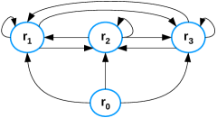
Figure 1: Firing graph of ${\mathcal{}P}_{\ref{ex:bubble}}$.

We say that a rule $r$ depends on a rule $r^{\prime}$ if $r$ can be reached from $r^{\prime}$ through the edges of $\Omega({\mathcal{}P})$. A strongly connected component (SCC) of a directed graph $G$ is a maximal set ${\mathcal{}C}$ of nodes of $G$ s.t. every node of ${\mathcal{}C}$ can be reached from every node of ${\mathcal{}C}$ (through the edges in $G$). We say that an SCC ${\mathcal{}C}$ is non-trivial if there exists at least one edge in $G$ between two not necessarily distinct nodes of ${\mathcal{}C}$. For instance, the firing graph in Figure 1 has two SCCs, ${\mathcal{}C}_{1}=\{r_{0}\}$ and ${\mathcal{}C}_{2}=\{r_{1},r_{2},r_{3}\}$, but only ${\mathcal{}C}_{2}$ is non-trivial. Given a program ${\mathcal{}P}$ and an SCC ${\mathcal{}C}$ of $\Omega({\mathcal{}P})$, $pred({\mathcal{}C})$ denotes the set of predicate symbols defined by the rules in ${\mathcal{}C}$. We now define when the head atom and a body atom of a rule are mutually recursive.

Definition 2 (Mutually recursive atoms)

Let ${\mathcal{}P}$ be a program and $r$ a rule in ${\mathcal{}P}$. The head atom $A=head(r)$ and an atom $B\in body(r)$ are mutually recursive if there is an SCC ${\mathcal{}C}$ of $\Omega({\mathcal{}P})$ s.t.:

1. ${\mathcal{}C}$ contains $r$, and

2. ${\mathcal{}C}$ contains a rule $r^{\prime}$ (possibly equal to $r$) s.t. $head(r^{\prime})$ and $B$ unify.  $\Box$

In the previous definition, when $r=r^{\prime}$ we assume that $r$ and $r^{\prime}$ are two “copies” that do not share any logical variable. Intuitively, the head atom $A$ of a rule $r$ and an atom $B$ in the body of $r$ are mutually recursive when there might be an actual propagation of terms from $A$ to $B$ (through the application of a sequence of rules). As a very simple example, if we have an SCC consisting only of the rule $\mathtt{p}(f(X))\leftarrow p(X),p(g(X))$, the first body atom is mutually recursive with the head, while the second one is not as it does not unify with the head atom.

Given a rule $r$, we use $rbody(r)$ to denote the set of atoms in $body(r)$ which are mutually recursive with $head(r)$. Moreover, we define $sbody(r)$ as the set consisting of every atom in $body(r)$ that contains all logical variables appearing in $head(r)$, and define $srbody(r)=rbody(r)\cap sbody(r)$.

We say that a rule $r$ in a program ${\mathcal{}P}$ is relevant if it is not a fact and the set of atoms $body(r)\setminus rbody(r)$ does not contain all logical variables in $head(r)$. Roughly speaking, a non-relevant rule will be ignored because either it cannot propagate terms or its head size is bounded by body atoms which are not mutually recursive with the head. We illustrate the notions introduced so far in the following example.

Example 4

Consider the following program ${\mathcal{}P}_{\ref{ex:simple_locally_bounded}}$:

$$\begin{array}[]{lll}r_{1}:\ \underbrace{\mathtt{s}(f(X),Y)}_{\text{A}}&\leftarrow&\mathtt{\underbrace{missing}}{\mathtt{q}(X,f(Y))}_{\text{B}},\ \underbrace{\mathtt{s}(Z,f(Y))}_{\text{C}}.\\ r_{2}:\ \underbrace{\mathtt{q}(f(U),V)}_{\text{D}}&\leftarrow&\mathtt{\underbrace{missing}}{\mathtt{s}(U,f(V))}_{\text{E}}.\\ \end{array}$$

The firing graph consists of the edges $\langle r_{1},r_{1}\rangle$, $\langle r_{1},r_{2}\rangle$, $\langle r_{2},r_{1}\rangle$. Thus, there is only one SCC ${\mathcal{}C}=\{r_{1},r_{2}\}$, which is non-trivial, and $pred({\mathcal{}C})=\mathtt{\{}q,s\}$. Atoms $A$ and $B$ (resp. $A$ and $C$, $D$ and $E$) are mutually recursive. Moreover, $rbody(r_{1})=\{B,C\}$, $srbody(r_{1})=\{B\}$, $rbody(r_{2})=srbody(r_{2})=\{E\}$. Both $r_{1}$ and $r_{2}$ are relevant.  $\Box$

We use $\mathbb{N}$ to denote the set of natural numbers $\{1,2,3,...\}$ and $\mathbb{N}_{0}$ to denote the set of natural numbers including the zero. Moreover, $\mathbb{N}^{k}=\{(v_{1},...,v_{k})\mid v_{i}\in\mathbb{N}\mbox{ for }1\leq i\leq k\}$ and $\mathbb{N}_{0}^{k}=\{(v_{1},...,v_{k})\mid v_{i}\in\mathbb{N}_{0}\mbox{ for }1\leq i\leq k\}$. Given a $k$-vector $\overline{v}=(v_{1},...,v_{k})$ in $\mathbb{N}_{0}^{k}$, we use $\overline{v}[i]$ to refer to $v_{i}$, for $1\leq i\leq k$. Given two $k$-vectors $\overline{v}=(v_{1},...,v_{k})$ and $\overline{w}=(w_{1},...,w_{k})$ in $\mathbb{N}_{0}^{k}$, we use $\overline{v}\cdot\overline{w}$ to denote the classical scalar product, i.e., $\overline{v}\cdot\overline{w}=\sum_{i=1}^{k}v_{i}\cdot w_{i}$.

As mentioned earlier, the basic idea of the proposed technique is to measure the size of terms and atoms in order to check if the rules’ head sizes are bounded when propagation occurs. Thus, we introduce the notions of term and atom size.

Definition 3

Let $t$ be a term. The size of $t$ is recursively defined as follows:

$$size(t)=\begin{cases}x&\mbox{ if }t\mbox{ is a logical variable\ }X;\\ m+\sum\limits_{i=1}^{m}size(t_{i})&\mbox{ if }t=f(t_{1},...,t_{m}).\end{cases}$$

where $x$ is an integer variable. The size of an atom $A=p(t_{1},...,p_{n})$, denoted $size(A)$, is the $n$-vector $(size(t_{1}),...,size(t_{n}))$.  $\Box$

In the definition above, an integer variable $x$ intuitively represents the possible sizes that the logical variable $X$ can have during the bottom-up evaluation. The size of a term of the form $f(t_{1},...,t_{m})$ is defined by summing up the size of its terms $t_{i}$’s plus the arity $m$ of $f$. Note that from the definition above, the size of every constant is 0.

Example 5

Consider rule $r_{1}$ of program ${\mathcal{}P}_{\ref{ex:bubble}}$ (see Example 1). Using $\mathtt{l}c$ to denote the list constructor operator “$|$”, the rule can be rewritten as follows:

$$\mathtt{b}ub(lc(Y,T),lc(X,Cur),Sol)\leftarrow\mathtt{b}ub(lc(X,lc(Y,T)),Cur,Sol),X\leq Y.$$

Let $A$ (resp. $B$) be the atom in the head (resp. the first atom in the body). Then,

$$\begin{array}[]{lll}\hskip 71.13188ptsize(A)&=&(2+y+t,\ \ 2+x+cur,\ \ sol)\\ \hskip 71.13188ptsize(B)&=&(2+[x+(2+y+t)],\ \ cur,\ \ sol)\hskip 71.13188pt\Box\end{array}$$

We are now ready to define rule-bounded programs.

Definition 4 (Rule-bounded programs)

Let ${\mathcal{}P}$ be a program, ${\mathcal{}C}$ a non-trivial SCC of $\Omega({\mathcal{}P})$, and $pred({\mathcal{}C})=\{p_{1},...,p_{k}\}$. We say that ${\mathcal{}C}$ is rule-bounded if there exist $k$ vectors $\overline{\alpha}_{p_{h}}\in\mathbb{N}^{\mathit{arity}(p_{h})}$, $1\leq h\leq k$, such that for every relevant rule $r\in{\mathcal{}C}$ with $A=head(r)=p_{i}(t_{1},...,t_{n})$, there exists an atom $B=p_{j}(u_{1},...,u_{m})$ in $srbody(r)$ s.t. the following inequality is satisfied

$$\overline{\alpha}_{p_{j}}\cdot size(B)-\overline{\alpha}_{p_{i}}\cdot size(A)\geq 0$$

for every non-negative value of the integer variables in $size(B)$ and $size(A)$.

We say that ${\mathcal{}P}$ is rule-bounded if every non-trivial SCC of $\Omega({\mathcal{}P})$ is rule-bounded.  $\Box$

Intuitively, for every relevant rule of a non-trivial SCC of $\Omega({\mathcal{}P})$, Definition 4 checks if the size of the head atom is bounded by the size of a mutually recursive body atom for all possible sizes the terms can assume.

Example 6

Consider again program ${\mathcal{}P}_{\ref{ex:simple_locally_bounded}}$ of Example 4. Recall that the only non-trivial SCC of $\Omega({\mathcal{}P}_{\ref{ex:simple_locally_bounded}})$ is ${\mathcal{}C}=\{r_{1},r_{2}\}$, and both $r_{1}$ and $r_{2}$ are relevant. To determine if the program is rule-bounded we need to check if ${\mathcal{}C}$ is rule-bounded. Thus, we need to find $\overline{\alpha}_{q},\overline{\alpha}_{s}\in\mathbb{N}^{2}$ such that there is an atom in $srbody(r_{1})$ and an atom in $srbody(r_{2})$ which satisfy the two inequalities derived from $r_{1}$ and $r_{2}$ for all non-negative values of the integer variables therein. Since both $srbody(r_{1})$ and $srbody(r_{2})$ contain only one element, we have only one choice, namely the one where $B$ is selected for $r_{1}$ and $E$ is selected for $r_{2}$.

Thus, we need to check if there exist $\overline{\alpha}_{q},\overline{\alpha}_{s}\in\mathbb{N}^{2}$ s.t. the following linear constraints are satisfied for all non-negative values of the integer variables appearing in them:

$$\begin{array}[]{lll}\!\begin{cases}\overline{\alpha}_{q}\cdot size(B)-\overline{\alpha}_{s}\cdot size(A)\geq 0\\ \overline{\alpha}_{s}\cdot size(E)-\overline{\alpha}_{q}\cdot size(D)\geq 0\end{cases}&\!\!\!\!\!\!\Rightarrow\!&\begin{cases}\overline{\alpha}_{q}\cdot(x,1+y)-\overline{\alpha}_{s}\cdot(1+x,y)\geq 0\\ \overline{\alpha}_{s}\cdot(u,1+v)-\overline{\alpha}_{q}\cdot(1+u,v)\geq 0\end{cases}\end{array}$$

By expanding the scalar products and isolating every integer variable we obtain:

$$\begin{cases}(\overline{\alpha}_{q}[1]-\overline{\alpha}_{s}[1])\cdot x+(\overline{\alpha}_{q}[2]-\overline{\alpha}_{s}[2])\cdot y+(\overline{\alpha}_{q}[2]-\overline{\alpha}_{s}[1])\geq 0\\ (\overline{\alpha}_{s}[1]-\overline{\alpha}_{q}[1])\cdot u+(\overline{\alpha}_{s}[2]-\overline{\alpha}_{q}[2])\cdot v+(\overline{\alpha}_{s}[2]-\overline{\alpha}_{q}[1])\geq 0\end{cases}$$

The previous inequalities must hold for all $x,y,u,v\in\mathbb{N}_{0}$; it is easy to see that this is the case iff the following system admits a solution:

$$\begin{cases}\begin{array}[]{lll}\overline{\alpha}_{q}[1]-\overline{\alpha}_{s}[1]\geq 0,&\ \ \overline{\alpha}_{q}[2]-\overline{\alpha}_{s}[2]\geq 0,&\ \ \overline{\alpha}_{q}[2]-\overline{\alpha}_{s}[1]\geq 0,\\ \overline{\alpha}_{s}[1]-\overline{\alpha}_{q}[1]\geq 0,&\ \ \overline{\alpha}_{s}[2]-\overline{\alpha}_{q}[2]\geq 0,&\ \ \overline{\alpha}_{s}[2]-\overline{\alpha}_{q}[1]\geq 0\end{array}\end{cases}$$

Since a solution does exist, e.g. $\overline{\alpha}_{s}[1]=\overline{\alpha}_{s}[2]=\overline{\alpha}_{q}[1]=\overline{\alpha}_{q}[2]=1$ (recall that every $\overline{\alpha}[i]$ must be greater than 0), the SCC ${\mathcal{}C}$ is rule-bounded, and so is the program.  $\Box$

The method in the previous example to find vectors $\overline{\alpha}_{p}$ for all $p\in pred({\mathcal{}C})$ can always be applied. That is, we can always isolate the integer variables in the original inequalities and then derive one inequality for each expression that multiplies an integer variable plus the one for the constant term, imposing that all such expressions must be greater than or equal to 0—we precisely state this property in Lemma 6.32.

It is worth noting that the proposed technique can easily recognize many terminating practical programs where terms are simply exchanged from the body to the head of rules (e.g., see Examples 1, 2, and 3).

Example 7

Consider program ${\mathcal{}P}_{\ref{ex:bubble}}$ of Example 1. Recall that the only non-trivial SCC of $\Omega({\mathcal{}P}_{\ref{ex:bubble}})$ is $\{r_{1},r_{2},r_{3}\}$ (see Figure 1) and all rules in it are relevant. Since $|srbody(r_{i})|=1$ for every $r_{i}$ in the SCC, we have only one set of inequalities, which is the following one after isolating integer variables(we assume that the empty list is represented by a simple constant):

$$\begin{cases}(\overline{\alpha}_{b}[1]-\overline{\alpha}_{b}[2])\cdot x_{1}+(2\overline{\alpha}_{b}[1]-2\overline{\alpha}_{b}[2])\geq 0\\ (\overline{\alpha}_{b}[1]-\overline{\alpha}_{b}[2])\cdot y_{2}+(2\overline{\alpha}_{b}[1]-2\overline{\alpha}_{b}[2])\geq 0\\ (\overline{\alpha}_{b}[1]-\overline{\alpha}_{b}[3])\cdot x_{3}+(\overline{\alpha}_{b}[2]-\overline{\alpha}_{b}[1])\cdot cur_{3}+(2\overline{\alpha}_{b}[1]-2\overline{\alpha}_{b}[3])\geq 0\end{cases}$$

where subscript $b$ stands for predicate symbol $\mathtt{b}ub$, whereas subscripts associated with integer variables are used to refer to the occurrences of logical variables in different rules (e.g., $y_{2}$ is the integer variable associated to the logical variable $\mathtt{Y}$ in rule $r_{2}$). A possible solution is $\overline{\alpha}_{{}_{b}}=(1,1,1)$ and thus ${\mathcal{}P}_{\ref{ex:bubble}}$ is rule-bounded.

Considering program ${\mathcal{}P}_{\ref{ex:visit}}$ of Example 2, we obtain the following constraints:

$$\begin{cases}(\overline{\alpha}_{v}[1]-\overline{\alpha}_{v}[2])\cdot root_{1}+(\overline{\alpha}_{v}[1]-\overline{\alpha}_{v}[3])\cdot right_{1}+(3\overline{\alpha}_{v}[1]-2\overline{\alpha}_{v}[2]-2\overline{\alpha}_{v}[3])\geq 0\\ (\overline{\alpha}_{v}[3]-\overline{\alpha}_{v}[1])\cdot next_{2}+2\overline{\alpha}_{v}[3]\geq 0\end{cases}$$

where subscript $v$ stands for predicate symbol $\mathtt{v}isit$. By setting $\overline{\alpha}_{v}=(2,1,2)$, we get positive integer values of $\overline{\alpha}_{v}[1],\overline{\alpha}_{v}[2],\overline{\alpha}_{v}[3]$ s.t. the inequalities above are satisfied for all $root_{1},$ $right_{1},$ $next_{2}\in\mathbb{N}_{0}$. Thus, ${\mathcal{}P}_{\ref{ex:visit}}$ is rule-bounded.

The firing graph of program ${\mathcal{}P}_{\ref{ex:append}}$ of Example 3 has two non-trivial SCCs ${\mathcal{}C}_{1}=\{r_{1}\}$ and ${\mathcal{}C}_{2}=\{r_{3}\}$. The constraints for ${\mathcal{}C}_{1}$ are:

$\begin{cases}(\overline{\alpha}_{r}[1]-\overline{\alpha}_{r}[2])\cdot x_{1}+(2\overline{\alpha}_{r}[1]-2\overline{\alpha}_{r}[2])\geq 0\end{cases}$

where subscript $r$ stands for predicate symbol $\mathtt{r}everse$. It is easy to see that by choosing any (positive integer) values of $\overline{\alpha}_{r}[1]$ and $\overline{\alpha}_{r}[2]$ such that $\overline{\alpha}_{r}[1]\geq\overline{\alpha}_{r}[2]$, the inequality above holds for all $x_{1}\in\mathbb{N}_{0}$. Likewise, the constraints for ${\mathcal{}C}_{2}$ are

$\begin{cases}(\overline{\alpha}_{a}[1]-\overline{\alpha}_{a}[2])\cdot x_{3}+(2\overline{\alpha}_{a}[1]-2\overline{\alpha}_{a}[2])\geq 0\end{cases}$

where subscript $a$ stands for predicate symbol $\mathtt{a}ppend$. By choosing any (positive integer) values of $\overline{\alpha}_{a}[1]$ and $\overline{\alpha}_{a}[2]$ such that $\overline{\alpha}_{a}[1]\geq\overline{\alpha}_{a}[2]$, the inequality above holds for all $x_{3}\in\mathbb{N}_{0}$. Thus, ${\mathcal{}P}_{\ref{ex:append}}$ is rule-bounded.  $\Box$

4 Correctness and expressiveness

In this section, we show that every rule-bounded program is terminating and provide results on the relative expressiveness of rule-bounded programs and other criteria.

Note that every program ${\mathcal{}P}$ can be partitioned into an ordered sequence of sub-programs ${\mathcal{}P}_{1},...,{\mathcal{}P}_{n}$, called stratification, such that, for every $1\leq i\leq n$, every rule $r$ in ${\mathcal{}P}_{i}$ depends only on rules belonging to some sub-program ${\mathcal{}P}_{j}$ with $1\leq j\leq i$. Recall that a rule $r$ depends on a rule $r^{\prime}$ if $r$ can be reached from $r^{\prime}$ through the edges of the firing graph. Moreover, there always exists a stratification where every sub-program ${\mathcal{}P}_{i}$ is either a non-trivial SCC or a set of trivial SCCs. Given a set of facts $D$, it is well known that ${\mathcal{}MM}({\mathcal{}P}\cup D)$ can be defined in terms of the minimal model of the ${\mathcal{}P}_{i}$’s following the order of the partition as follows: if $M_{0}=D$ and $M_{i}={\mathcal{}MM}({\mathcal{}P}_{i}\cup M_{i-1})$ for $1\leq i\leq n$, then $M_{n}={\mathcal{}MM}({\mathcal{}P}\cup D)$.

Lemma 1

A program ${\mathcal{}P}$ is terminating iff every non-trivial SCC of $\Omega({\mathcal{}P})$ is terminating.

Proof 4.1.

($\Rightarrow$) Clearly, if there is an SCC which is not terminating, then ${\mathcal{}P}$ is not terminating.

($\Leftarrow$) Assume now that ${\mathcal{}P}$ does not terminate and all its non-trivial SCCs terminates. This means that there is a set of facts $D$ such that the fixpoint of ${\mathcal{}P}\cup D$ is not finite. Since ${\mathcal{}P}\cup D$ can be partitioned into $({\mathcal{}P}_{1},...,{\mathcal{}P}_{n})$, there must be a non-trivial (i.e. recursive) SCC ${\mathcal{}P}_{i}$ such that ${\mathcal{}P}_{i}\cup M_{i-1}$ does not terminate. This contradicts the hypothesis that all non-trivial SCCs terminate. Indeed if $P_{i}$ terminates, then for every set of facts $D^{\prime}$ including the facts in $M_{i-1}$, the fixpoint of ${\mathcal{}P}_{i}\cup D^{\prime}$ terminates and, therefore, the fixpoint of ${\mathcal{}P}_{i}\cup M_{i-1}$ terminates as well.

We now refine the previous lemma by showing that to see if a program ${\mathcal{}P}$ is terminating it is not necessary to analyze every non-trivial SCC entirely, but we can focus on its relevant rules. Henceforth, for every set of rules ${\mathcal{}C}$, we use $Rel({\mathcal{}C})$ to denote the set of relevant rules of ${\mathcal{}C}$.

Lemma 4.2.

Let ${\mathcal{}P}$ be a program and let ${\mathcal{}C}$ be an SCC of $\Omega({\mathcal{}P})$. Then, ${\mathcal{}C}$ is terminating iff $Rel({\mathcal{}C})$ is terminating.

Proof 4.3.

It follows from the fact that we can derive only a finite number of ground atoms using the rules in $ground({\mathcal{}C})\setminus ground(Rel({\mathcal{}C}))$ starting from a finite set of facts—recall that, by definition, every non-relevant rule has a set of atoms in the body that are not mutually recursive with the head and contain all variables in the head.

To show the correctness of our approach, we first show that every rule-bounded program can be rewritten into an “equivalent” program belonging to a simpler class of programs, called size-bounded. Then, we prove that size-bounded programs are terminating and this entails that rule-bounded programs are terminating as well.

Definition 4.4 (Program expansion).

Let ${\mathcal{}P}$ be a program and let $\omega=\{\overline{\omega}_{p_{1}},...,\overline{\omega}_{p_{n}}\}$ be a set of vectors such that $\overline{\omega}_{p_{i}}\in\mathbb{N}^{\mathit{arity}(p_{i})}$ and $p_{i}\in pred({\mathcal{}P})$ for $1\leq i\leq n$. For any atom $A=p(t_{1},...,t_{m})$ occurring in ${\mathcal{}P}$, we define $A^{\omega}=A$, if $p\not\in pred({\mathcal{}P})$, otherwise $A^{\omega}=p(\overline{t}_{1},...,\overline{t}_{m})$, where each $\overline{t}_{j}$ is the sequence $t_{j},...,t_{j}$ of length $\omega_{p}[j]$. Finally, ${\mathcal{}P}^{\omega}$ denotes the program derived from ${\mathcal{}P}$ by replacing every atom $A$ with $A^{\omega}$. $\Box$

Intuitively, the expansion of a program is obtained from the original program by increasing the arity of each predicate symbol according to $\omega$. Below is an example.

Example 4.5.

Consider program $P_{\ref{ex:simple_locally_bounded}}$ of Example 4 and the set of vectors $\omega=\{\overline{\omega}_{\mathtt{s}},\overline{\omega}_{\mathtt{q}}\}$ where $\overline{\omega}_{\mathtt{s}}=(2,3)$ and $\overline{\omega}_{\mathtt{q}}=(2,1)$. The program $P_{\ref{ex:simple_locally_bounded}}^{\omega}$ is as follows:

$$\begin{array}[]{lll}\hskip 28.45274ptr_{1}:\mathtt{\ }s(f(X),f(X),Y,Y,Y)&\leftarrow&\mathtt{q}(X,X,f(Y)),\ \ s(Z,Z,f(Y),f(Y),f(Y)).\\ \hskip 28.45274ptr_{2}:\mathtt{\ }q(f(U),f(U),V)&\leftarrow&\mathtt{s}(U,U,f(V),f(V),f(V)).\hskip 85.35826pt\Box\end{array}$$

We now show that for every program ${\mathcal{}P}$ and every set of vectors $\omega$, ${\mathcal{}P}$ is terminating iff ${\mathcal{}P}^{\omega}$ is terminating. In the following, for every program ${\mathcal{}P}$, we define $\omega({\mathcal{}P})=\{\ \{\overline{\omega}_{p_{1}},...,\overline{\omega}_{p_{n}}\}\mid p_{i}\in pred({\mathcal{}P})\wedge\overline{\omega}_{p_{i}}\in\mathbb{N}^{\mathit{arity}(p_{i})}\}$.

Lemma 4.6.

For every program ${\mathcal{}P}$ and every $\omega\in\omega({\mathcal{}P})$, ${\mathcal{}P}$ is terminating iff ${\mathcal{}P}^{\omega}$ is terminating.

Proof 4.7.

For every atom $A^{\omega}$ occurring in ${\mathcal{}P}^{\omega}$ let $A$ be the corresponding atom in ${\mathcal{}P}$. The claim follows from the observation that whenever there is a instance $D$ such that $\mathit{T}_{{\mathcal{}P}\cup D}^{\infty}(\emptyset)$ is infinite, it is always possible to construct the instance $D^{\omega}$ which guarantees that $\mathit{T}_{{\mathcal{}P}^{\omega}\cup D^{\omega}}^{\infty}(\emptyset)$ is infinite as well.
Conversely, for every instance $D^{\omega}$ of ${\mathcal{}P}^{\omega}$, if $\mathit{T}_{{\mathcal{}P}^{\omega}\cup D^{\omega}}^{\infty}(\emptyset)$ is infinite, then we can always construct the instance $D$ guaranteeing that $\mathit{T}_{{\mathcal{}P}\cup D}^{\infty}(\emptyset)$ is infinite as well.

We now introduce the class of size-bounded programs and show that such programs are terminating. To this aim, we define the total size of an atom $A=p(t_{1},...,t_{n})$ as $tsize(A)=\sum\limits_{i=1}^{n}size(t_{i})$.

Definition 4.8 (Size-bounded program).

A program ${\mathcal{}P}$ is said to be size-bounded if for every rule $r\in{\mathcal{}P}$ which is not a fact, there is an atom $B$ in $sbody(r)$ such that $tsize(B)\geq tsize(head(r))$ for every non-negative value of the integer variables occurring in $tsize(B)$ and $tsize(head(r))$.

Theorem 4.9.

Every size-bounded program is terminating.

Proof 4.10.

Let ${\mathcal{}P}$ be a size-bounded program and $D$ a finite set of facts, we consider only rules in ${\mathcal{}P}$ having a non-empty body. Given an atom $A$ and a ground instance $A^{\prime}$ of $A$, let $\theta$ be the mgu of $A$ and $A^{\prime}$. Notice that $\theta$ is of the form $\{X_{1}/t_{1},...,X_{n}/t_{n}\}$ where the $X_{i}$’s are exactly the logical variables occurring in $A$ and all the $t_{j}$’s are ground terms. It can be easily verified that $tsize(A^{\prime})$ can be obtained from $tsize(A)$ by replacing every integer variable $x_{i}$ in $tsize(A)$ with $size(t_{i})$.

We now show that for every ground rule $r^{\prime}\in ground({\mathcal{}P})$ there is an atom $B^{\prime}\in body(r^{\prime})$ such that $tsize(B^{\prime})\geq tsize(head(r^{\prime}))$. Consider a rule $r$ in ${\mathcal{}P}$ of the form $A\leftarrow B_{1},...,B_{k}$ and a ground rule $r^{\prime}\in ground(r)$ of the form $A^{\prime}\leftarrow B_{1}^{\prime},...,B_{k}^{\prime}$. Since ${\mathcal{}P}$ is size-bounded, there exists an atom $B_{j}$ in $sbody(r)$ such that $tsize(B_{j})\geq tsize(A)$ for every non-negative value of the integer variables occurring in the inequality. Notice every logical variable in $A$ appears also in $B_{j}$ by definition of $sbody$. Let $\{X_{1}/t_{1},...,X_{n}/t_{n}\}$ be the mgu of $B_{j}$ and $B_{j}^{\prime}$. As $tsize(B_{j})\geq tsize(A)$ holds for all non-negative value of its integer variables, it also holds when every integer variable $x_{i}$ is replaced with $size(t_{i})$, for $1\leq i\leq n$. Thus, $tsize(B_{j}^{\prime})\geq tsize(A^{\prime})$.

Let us denote $\mathit{T}_{{\mathcal{}P}\cup D}^{i}(\emptyset)$ as $M_{i}$ for every $i\geq 1$ and let $tsize_{max}=\max\{tsize(B)\mid B\leftarrow\mbox{ is a fact in }{\mathcal{}P}\cup D\}$. We show that for every $i\geq 1$ and every ground atom $A$ in $M_{i}$ the following holds $tsize_{max}\geq tsize(A)$. The proof is by induction on $i$.

$\bullet$ Base case ($i$=$1$). It follows from the fact that $M_{1}$=$\{B\mid B\!\leftarrow\!\mbox{ is a fact in }{\mathcal{}P}\,\cup\,D\}$.

$\bullet$ Inductive step ($i\rightarrow i+1$). Let $r^{\prime}$ be a ground rule in $ground({\mathcal{}P})$ such that $body(r^{\prime})\subseteq M_{i}$. Then, as shown above, there is an atom $B$ in $body(r^{\prime})$ such that $tsize(B)\geq tsize(head(r^{\prime}))$. By the induction hypothesis, $tsize_{max}\geq tsize(B)$ and thus $tsize_{max}\geq tsize(head(r^{\prime}))$.

Thus, for every $i\geq 1$ and every ground atom $A$ in $M_{i}$, we have that $tsize(A)$ is bounded by $tsize_{max}$. Since programs are range-restricted, atoms in $\cup_{i\geq 1}M_{i}$ are built from constants and function symbols appearing in ${\mathcal{}P}\cup D$, which are finitely many. These observations and the definition of $tsize$ imply that we can have only finitely many ground atoms in $\cup_{i\geq 1}M_{i}$. Hence, ${\mathcal{}P}$ is terminating.

We are now ready to show the correctness of the rule-bounded technique.

Theorem 4.11.

Every rule-bounded program is terminating.

Proof 4.12.

Let ${\mathcal{}P}$ be a rule-bounded program and ${\mathcal{}C}$ a non-trivial SCC of $\Omega({\mathcal{}P})$. Since ${\mathcal{}P}$ is rule-bounded, then there exists $\omega\in\omega({\mathcal{}C})$ which satisfies the condition of Definition 4, that is, ${\mathcal{}C}$ is rule-bounded. This implies that $Rel({\mathcal{}C})^{\omega}$ is size-bounded. Thus, $Rel({\mathcal{}C})^{\omega}$ is terminating by Theorem 4.9. Lemma 4.6 implies that $Rel({\mathcal{}C})$ is terminating and Lemma 4.2 in turn implies that ${\mathcal{}C}$ is terminating. Finally, by Lemma 1, we can conclude that ${\mathcal{}P}$ is terminating.

The class of rule-bounded programs is incomparable with different termination criteria in the literature, including the most general ones.

Theorem 4.13.

Rule-bounded programs are incomparable with argument-restricted, mapping-re-stricted, and bounded programs.

Proof 4.14.

Recall that both bounded and mapping-restricted programs include argument-restricted programs. To prove the claim we show that (i) there is a program which is rule-bounded but is neither mapping-restricted nor bounded, and (ii) there is a program which is argument-restricted but not rule-bounded. (i) As already shown, program ${\mathcal{}P}_{\ref{ex:bubble}}$ of Example 1 is rule-bounded; however, it can be easily verified that ${\mathcal{}P}_{\ref{ex:bubble}}$ is neither mapping-restricted nor bounded. (ii) Consider the program consisting of the rules $\mathtt{p}(f(X))\leftarrow q(X)$ and $\mathtt{q}(Y)\leftarrow p(f(Y))$. This program is argument-restricted (and thus also mapping-restricted and bounded) but is not rule-bounded.

Regarding the termination criteria mentioned in Theorem 4.13, we recall that mapping restriction $(MR)$ and bounded programs $(BP)$ are incomparable and both extend argument restriction $(AR)$. Concerning the computational complexity, while $AR$ is polynomial time, both $MR$ and $BP$ are exponential. As a remark, it is interesting to note that the above result highlights the fact that our technique analyzes logic programs from a radically different point of view w.r.t. previously defined approaches, which analyze how complex terms are propagated among arguments.

5 Cycle-bounded Programs

As saw in the previous section, to determine if a program is rule-bounded we check through linear constraints if the size of the head atom is bounded by the size of a body atom for every relevant rule in a non-trivial SCC of the firing graph (cf. Definition 4). Looking at each rule individually has its limitations, as shown by the following example.

Example 5.15.

Consider the following simple program ${\mathcal{}P}_{\ref{ex:globally-bounded}}$:

$$\begin{array}[]{lll}r_{1}:\ \mathtt{p}(X,Y)&\leftarrow&\mathtt{q}(f(X),Y).\\ r_{2}:\ \mathtt{q}(W,f(Z))&\leftarrow&\mathtt{p}(W,Z).\end{array}$$

It is easy to see that the program above is terminating, but it is not rule-bounded. The linear inequalities for the program are (cf. Definition 4):

$$\begin{cases}(\overline{\alpha}_{q}[1]-\overline{\alpha}_{p}[1])\cdot x+(\overline{\alpha}_{q}[2]-\overline{\alpha}_{p}[2])\cdot y+\overline{\alpha}_{q}[1]\geq 0\\ (\overline{\alpha}_{p}[1]-\overline{\alpha}_{q}[1])\cdot w+(\overline{\alpha}_{p}[2]-\overline{\alpha}_{q}[2])\cdot z-\overline{\alpha}_{q}[2]\geq 0\end{cases}$$

It can be easily verified that there are no positive integer values for $\overline{\alpha}_{p}[1],$ $\overline{\alpha}_{p}[2],$ $\overline{\alpha}_{q}[1],$ $\overline{\alpha}_{q}[2]$ such that the inequalities hold for all $x,y,w,z\in\mathbb{N}_{0}$. The reason is the presence of the expression $-\overline{\alpha}_{q}[2]$ in the second inequality. Intuitively, this is because the size of the head atom increases w.r.t. the size of the body atom in $r_{2}$. However, notice that the cycle involving $r_{1}$ and $r_{2}$ does not increase the overall size of propagated terms. This suggests we can check if an entire cycle (rather than each individual rule) propagates terms of bounded size.  $\Box$

To deal with programs like the one shown in the previous example, we introduce the class of cycle-bounded programs, which is able to perform an analysis of how terms propagate through a group of rules, rather than looking at rules individually as done by the rule-bounded criterion.

Given a program ${\mathcal{}P}$, a cyclic path $\pi$ of $\Omega({\mathcal{}P})$ is a sequence of edges $\langle r_{1},r_{2}\rangle,\langle r_{2},r_{3}\rangle,$ $...,\langle r_{n},r_{1}\rangle$. Moreover a cyclic path $\pi$ is basic if every edge $\pi$ does not occur more than once. We say that $\pi$ is relevant if every $r_{i}$ is relevant, for $1\leq i\leq n$.

In the following, we first present the cycle-bounded criterion for linear programs and then show how it can be applied to non-linear ones.

Dealing with linear programs.

A program ${\mathcal{}P}$ is linear if every rule in ${\mathcal{}P}$ is linear. A rule $r$ is linear if $|rbody(r)|\leq 1$. Notice that $rbody(r)$ contains exactly one atom $B$ for every linear rule $r$ in a non-trivial SCC of the firing graph; thus, with a slight abuse of notation, we use $rbody(r)$ to refer to $B$.

Definition 5.16 (Cycle constraints).

Let ${\mathcal{}P}$ be a linear program and let $\pi=\langle r_{1},r_{2}\rangle,...,\langle r_{n},r_{1}\rangle$ be a basic cyclic path of $\Omega({\mathcal{}P})$. For every mgu $\theta_{i}$ of $head(r_{i})$ and $rbody(r_{i+1})$ ($1\leq i<n$), we define the set of (linear) equalities $eq(\theta_{i})=\{x=size(t)\mid X/t\in\theta_{i}\}$. Then, we define $eq(\pi)=\bigcup\limits_{1\leq i<n}eq(\theta_{i})$.   $\Box$

Example 5.17.

Consider the program ${\mathcal{}P}_{\ref{ex:globally-bounded}}$ and the two basic cyclic paths $\pi_{1}=\langle r_{1},r_{2}\rangle\,\langle r_{2},r_{1}\rangle$ and $\pi_{2}=\langle r_{2},r_{1}\rangle\,\langle r_{1},r_{2}\rangle$ of $\Omega({\mathcal{}P}_{\ref{ex:globally-bounded}})$. The mgu of $head(r_{1})$ and $rbody(r_{2})$ is $\theta=\{\mathtt{X}/W,\ Y/Z\}$ and thus $eq(\pi_{1})=\{x=w,\ y=z\}$. Furthermore, the mgu of $head(r_{2})$ and $rbody(r_{1})$ is $\theta=\{\mathtt{W}/f(X),\ Y/f(Z)\}$ and thus $eq(\pi_{2})=\{w=1+x,\ y=1+z\}$.  $\Box$

Definition 5.18 (Linear cycle-bounded programs).

Let ${\mathcal{}P}$ be a linear program, $\pi=\langle r_{1},r_{2}\rangle\,...\,\langle r_{n},r_{1}\rangle$ be a basic cyclic path of $\Omega({\mathcal{}P})$ and $p$ be the predicate defined by $r_{n}$. We say that $\pi$ is cycle-bounded if $eq(\pi)$ is satisfiable for some non-negative value of its integer variables and there exists a vector $\overline{\alpha}_{p}\in\mathbb{N}^{\mathit{arity}(p)}$ such that the constraint

$$\overline{\alpha}_{p}\cdot size(rbody(r_{1}))-\overline{\alpha}_{p}\cdot size(head(r_{n}))\geq 0$$

is satisfied for every non-negative value of its integer variables that satisfy $eq(\pi)$. We say that ${\mathcal{}P}$ is cycle-bounded if every relevant basic cyclic path of $\Omega({\mathcal{}P})$ is cycle-bounded.  $\Box$

In the definition above, we assume that distinct basic cyclic paths do not share any logical variable.

Example 5.19.

Consider again program ${\mathcal{}P}_{\ref{ex:globally-bounded}}$ of Example 5.15. The program is clearly linear and $\Omega({\mathcal{}P}_{\ref{ex:globally-bounded}})$ has only two relevant basic cyclic paths $\pi_{1}=\langle r_{1},r_{2}\rangle\langle r_{2},r_{1}\rangle$ and $\pi_{2}=\langle r_{2},r_{1}\rangle\langle r_{1},r_{2}\rangle$. To check if ${\mathcal{}P}_{\ref{ex:globally-bounded}}$ is cycle-bounded, we need to check if $eq(\pi_{1})=\{x_{1}=w_{1},\ y_{1}=z_{1}\}$ and $eq(\pi_{2})=\{w_{2}=1+x_{2},\ y_{2}=1+z_{2}\}$ admit a solution and if there exist $\overline{\alpha}_{p},\overline{\alpha}_{q}\in\mathbb{N}^{2}$ s.t. the constraints:

$$\begin{array}[]{llll}\overline{\alpha}_{q}\cdot(x_{1}+1,y_{1})&-&\overline{\alpha}_{q}\cdot(w_{1},z_{1}+1)&\geq 0,\\ \overline{\alpha}_{p}\cdot(w_{2},z_{2})&-&\overline{\alpha}_{p}\cdot(x_{2},y_{2})&\geq 0\end{array}$$

are satisfied for all $x_{1},y_{1},w_{1},z_{1}\in\mathbb{N}_{0}$ and all $x_{2},y_{2},w_{2},z_{2}\in\mathbb{N}_{0}$ that satisfy $eq(\pi_{1})$ and $eq(\pi_{2})$.

By applying the equality conditions $eq(\pi_{1})$ and $eq(\pi_{2})$ to the above constraints we get the below inequalities for the basic cyclic paths $\pi_{1}$ and $\pi_{2}$:

$$\begin{array}[]{llll}(\overline{\alpha}_{q}[1],\overline{\alpha}_{q}[2])\cdot(x_{1}+1,z_{1})&-&(\overline{\alpha}_{q}[1],\overline{\alpha}_{q}[2]))\cdot(x_{1},z_{1}+1)&\geq 0,\\ (\overline{\alpha}_{p}[1],\overline{\alpha}_{p}[2]))\cdot(x_{2}+1,z_{2})&-&(\overline{\alpha}_{p}[1],\overline{\alpha}_{p}[2]))\cdot(x_{2},z_{2}+1)&\geq 0\end{array}$$

It is easy to see that the first constraint (resp. the second) is satisfied for every vector $\overline{\alpha}_{p}\in\mathbb{N}^{2}$ (resp. $\overline{\alpha}_{q}\in\mathbb{N}^{2}$) such that $\overline{\alpha}_{p}[1]\geq\overline{\alpha}_{p}[2]$ (resp. $\overline{\alpha}_{q}[1]\geq\overline{\alpha}_{q}[2]$). Thus, ${\mathcal{}P}_{\ref{ex:globally-bounded}}$ is cycle-bounded.   $\Box$

To prove the correctness of our approach, we introduce a simpler class of terminating programs, as we did in the case of rule-bounded programs.

Definition 5.20 (Linear cycle-size-bounded programs).

Let ${\mathcal{}P}$ be a linear program. We say that ${\mathcal{}P}$ is cycle-size-bounded if for every relevant basic cyclic path $\pi=\langle r_{1},r_{2}\rangle\,...\,\langle r_{n},r_{1}\rangle$ of $\Omega({\mathcal{}P})$, $eq(\pi)$ is satisfiable for some non-negative value of its integer variables and the constraint

$$tsize(rbody(r_{1}))-tsize(head(r_{n}))\geq 0$$

is satisfied for every non-negative value of its integer variables that satisfy $eq(\pi)$.  $\Box$

Theorem 5.21.

Every linear cycle-size-bounded program is terminating.

Proof 5.22.

Let ${\mathcal{}P}$ be a cycle-size-bounded program and $D$ a finite set of facts. Consider a relevant basic cyclic path $\pi=\langle r_{1},r_{2}\rangle\,...\,\langle r_{n},r_{1}\rangle$ of $\Omega({\mathcal{}P})$. Let $r_{1}^{\prime},...,r_{n}^{\prime}$ be ground rules s.t. $r_{i}^{\prime}\in ground(r_{i})$ for $1\leq i\leq n$ and $head(r_{i}^{\prime})=rbody(r_{i+1}^{\prime})$ for $1\leq i<n$. For $1\leq i\leq n$, let $\theta^{h}_{i}$ be the mgu of $head(r_{i})$ and $head(r_{i}^{\prime})$, and $\theta^{b}_{i}$ the mgu of $rbody(r_{i})$ and $rbody(r_{i}^{\prime})$. Then,

$\bullet$ $tsize(head(r_{i}^{\prime}))$ can be obtained from $tsize(head(r_{i}))$ by replacing every integer variable $x$ in $tsize(head(r_{i}))$ with $size(t)$ provided that $X/t\in\theta^{h}_{i}$, for $1\leq i\leq n$;

$\bullet$ $tsize(rbody(r_{i}^{\prime}))$ can be obtained from $tsize(rbody(r_{i}))$ by replacing every integer variable $x$ in $tsize(rbody(r_{i}))$ with $size(t)$ provided that $X/t\in\theta^{b}_{i}$, for $1\leq i\leq n$;

$\bullet$ if we replace every integer variable $x$ in $eq(\pi)$ with $size(t)$ iff $X/t$ belongs to $\cup_{i=1}^{n}(\theta^{h}_{i}\cup\theta^{b}_{i})$, then $eq(\pi)$ is satisfied.

The items above entail that $tsize(rbody(r_{1}^{\prime}))-tsize(head(r_{n}^{\prime}))\geq 0$. This means that we cannot derive atoms of increasing size through the cyclic application of rules and thus ${\mathcal{}P}\cup D$ is terminating.

Theorem 5.23 (Soundness).

Every linear cycle-bounded program is terminating.

Proof 5.24.

The proof is similar to the one presented for rule-bounded programs. Given a linear cycle-bounded program ${\mathcal{}P}$, we are going to construct an equivalent program (like ${\mathcal{}P}^{\omega}$) to ${\mathcal{}P}$ as follows: for every relevant basic cyclic path $\pi=\langle r_{1},r_{2}\rangle\,...\,\langle r_{n},r_{1}\rangle$ of $\Omega({\mathcal{}P})$, let $\overline{\alpha}_{p}$ be the vector such that $\overline{\alpha}_{p}\cdot size(rbody(r_{1}))-\overline{\alpha}_{p}\cdot size(head(r_{n}))\geq 0$. Then, remove rules $r_{1}$ and $r_{n}$ from ${\mathcal{}P}$ and insert the rules $head(r_{1})\leftarrow rbody(r_{1})^{\overline{\alpha}_{p}}$ and $head(r_{n})^{\overline{\alpha}_{p}}\leftarrow rbody(r_{n})$ respectively. Finally, in order to preserve the activation of rules in the obtained program, for every pair of basic cyclic paths $\pi_{1}=\langle r_{1},r_{2}\rangle\,...\,\langle r_{n},r_{1}\rangle$, $\pi_{2}=\langle s_{1},s_{2}\rangle\,...\,\langle s_{m},s_{1}\rangle$, where $p$ is the predicate defined by $r_{n}$ and $s_{n}$ with arity $k$, add to ${\mathcal{}P}$ a rule of the form $A^{\overline{\alpha}_{p}}\leftarrow A^{\overline{\beta}_{p}}$, where $A$ is the atom $p(X_{1},...,X_{k})$ and $\overline{\alpha}_{p}$, $\overline{\beta}_{p}$ are the vectors such that $\overline{\alpha}_{p}\cdot size(rbody(r_{1}))-\overline{\alpha}_{p}\cdot size(head(r_{n}))\geq 0$ and $\overline{\beta}_{p}\cdot size(rbody(s_{1}))-\overline{\beta}_{p}\cdot size(head(s_{m}))\geq 0$ respectively. It is not difficult to show that the obtained program is terminating iff ${\mathcal{}P}$ is terminating. Moreover, since ${\mathcal{}P}$ is cycle-bounded the new program is consequently cycle-size-bounded. From Theorem 5.21, we get that the new program is terminating and so it is ${\mathcal{}P}$.

Dealing with non-linear programs.

The application of the cycle-bounded criterion to arbitrary programs consists in applying the technique to a set of linear programs derived from the original one. Given a rule $r$, the set of linear versions of $r$ is defined as the set of rules $\ell(r)=\{head(r)\leftarrow B\mid B\in rbody(r)\}$. Given a program ${\mathcal{}P}=\{r_{1},...,r_{n}\}$, the set of linear versions of ${\mathcal{}P}$ is defined as the set of linear programs $\ell({\mathcal{}P})=\{\{r_{1}^{\prime},...,r_{n}^{\prime}\}\mid r_{i}^{\prime}\in\ell(r_{i})\mbox{ for }1\leq i\leq n\}$.

Definition 5.25 (Cycle-bounded programs).

A (possibly non-linear) program ${\mathcal{}P}$ is cycle-bounded if every (linear) program in $\ell({\mathcal{}P})$ is cycle-bounded.  $\Box$

Theorem 5.26.

Every cycle-bounded program is terminating.

Proof 5.27.

Notice that every linear version ${\mathcal{}P}^{\prime}\in\ell({\mathcal{}P})$ of ${\mathcal{}P}$ is such that for every set of facts $D$, ${\mathcal{}MM}(D\cup{\mathcal{}P})\subseteq{\mathcal{}MM}(D\cup{\mathcal{}P}^{\prime})$. Thus, if every linear version of ${\mathcal{}P}$ is cycle-bounded  then for every set of facts $D$, ${\mathcal{}MM}(D\cup{\mathcal{}P})$ is finite.

Theorem 5.28 (Expressivity).

Cycle-bounded programs are incomparable with rule-bounded, argument-restricted, mapping-restricted and bounded programs.

Proof 5.29.

As shown in Example 5.15, program ${\mathcal{}P}_{\ref{ex:globally-bounded}}$ is cycle-bounded, but it can be easily verified that it is neither mapping-restricted (and thus not argument-restricted) nor rule-bounded. Moreover, the one rule program $\{\mathtt{p}(X,Y,f(Z,W))\leftarrow p(f(Z,Y),X,W).\}$ is cycle-bounded but it is not bounded.
Conversely, the program $\{\mathtt{p}(f(X))\leftarrow p(f(f(X))),p(X).\}$ is rule-bounded, argument-restricted (and thus mapping-restricted) and bounded but not cycle-bounded.

6 Complexity

In this section, we provide upper bounds for the time complexity of checking whether a program is rule-bounded or cycle-bounded. We assume that constant space is used to store each constant, logical variable, function symbol, and predicate symbol. The syntactic size of a term $t$ (resp. atom, rule, program), denoted by $||t||$, is the number of symbols occurring in $t$, except for the symbols “(”, “)”, “,”, “.”, and “$\leftarrow$”. Thus, in this section, the complexity of a problem involving ${\mathcal{}P}$ is assumed to be w.r.t. $||{\mathcal{}P}||$. Obviously $|{\mathcal{}P}|=O(||{\mathcal{}P}||)$.

Lemma 6.30.

Given a program ${\mathcal{}P}$, constructing $\Omega({\mathcal{}P})$ is in $\mathit{PTIME}$.

Proof 6.31.

The construction of $\Omega({\mathcal{}P})$ requires checking, for every atom $A$ in the head of a rule and every atom $B$ in the body of a rule, if $A$ and $B$ unify. Since we need to check $|{\mathcal{}P}|\times\sum_{r\in{\mathcal{}P}}|body(r)|$ times if two atoms unify and checking whether two atoms $A$ and $B$ unify can be done in quadratic time w.r.t. $||A||$ and $||B||$ [Venturini Zilli (1975)], then the construction of $\Omega({\mathcal{}P})$ is in $\mathit{PTIME}$.

It is worth noting that the number of SCCs is bounded by $O(|{\mathcal{}P}|)$ and that after having built $\Omega({\mathcal{}P})$, the cost of checking whether a SSC is trivial or nontrivial is constant, whereas the cost of checking whether a rule is relevant is bounded by $O(||{\mathcal{}P}||)$. Inequalities associated with basic cycles can be rewritten by grouping terms with respect to integer coefficients (also called $\alpha$-coefficients) or with respect to integer variables. Therefore, in the following we assume that inequalities grouped with respect to integer variables are of the form $\gamma_{1}\cdot x_{1},+\cdots+\gamma_{n}\cdot x_{n}+\gamma_{0}\geq 0,$ where each $\gamma_{i}$, for $0\leq i\leq n$, is an arithmetic expression built by using $\alpha$-coefficients and natural numbers, whereas inequalities grouped with respect to integer coefficients are of the form $\alpha_{1}\cdot w_{1},+\cdots+\alpha_{m}\cdot w_{m}\geq 0,$ where each $w_{j}$, for $1\leq i\leq m$, is an arithmetic expression built by using integer variables and natural numbers. Obviously, each $\gamma_{i}$ can be considered an integer coefficient, whereas each $w_{j}$ can be considered an integer variable.

Lemma 6.32.

Consider a linear inequality of the form

$$\gamma_{1}\cdot x_{1}+...+\gamma_{n}\cdot x_{n}+\gamma_{0}\geq 0$$

where the $\gamma_{i}$’s are integer coefficients and the $x_{j}$’s are integer variables. The inequality is satisfied for every non-negative value of the $x_{j}$’s iff $\gamma_{i}\geq 0$ for every $0\leq i\leq n$.

Proof 6.33.

($\Leftarrow$) Straightforward. ($\Rightarrow$) By contradiction, assume that the inequality is satisfied for every non-negative value of the integer variables occurring in it, but there exists $0\leq i\leq n$ such that $\gamma_{i}<0$. If $1\leq i\leq n$, then the inequality is not satisfied when $x_{i}=\lfloor abs(\gamma_{n+1}/\gamma_{i})\rfloor+1$ and $x_{j}=0$ for every $j\neq i$. If $i=0$, then the inequality is not satisfied when $x_{j}=0$ for every $1\leq j\leq n$.

Theorem 6.34.

Checking whether a program ${\mathcal{}P}$ is rule-bounded is in $\mathit{NP}$.

Proof 6.35.

In order to check whether ${\mathcal{}P}$ is rule-bounded we need to: 1) construct the firing graph $\Omega({\mathcal{}P})$ of ${\mathcal{}P}$, 2) compute the SCCs of $\Omega({\mathcal{}P})$, and 3) check if every non-trivial SCC is rule-bounded.

1) The construction of the firing graph is in $\mathit{PTIME}$ by Lemma 6.30.
2) It is well known that computing the SCCs of a directed graph can be done in linear time w.r.t. the number of nodes and edges. Since the number of nodes of $\Omega({\mathcal{}P})$ is $|{\mathcal{}P}|$ and the maximum number of edges of $\Omega({\mathcal{}P})$ is $|{\mathcal{}P}|^{2}$, then computing all the SCCs is clearly in $\mathit{PTIME}$.
3) Let ${\mathcal{}C}$ be a non-trivial SCC of $\Omega({\mathcal{}P})$, $n=O(|{\mathcal{}P}|)$ the number of relevant rules in ${\mathcal{}C}$, $v$ the maximum number of distinct variables occurring in the head atoms of the relevant rules in ${\mathcal{}C}$, and $a$ the maximum arity of the predicate symbols in $pred({\mathcal{}C})$. Since it is always possible to rewrite the constraints as in Definition 4 in the form presented by Lemma 6.32, given a fixed choice of one atom in $srbody(r)$ for every relevant rule $r$ of ${\mathcal{}C}$, checking whether ${\mathcal{}C}$ is rule-bounded according to that choice can be done by solving a set of at most $n\times(v+1)$ linear constraints with at most $2\times a$ non-negative coefficients per constraint—clearly, the size of the set of constraints is bounded by $O(||{\mathcal{}P}||)$ and if the set of constraints admit a solution, then there is a solution where the size of the $\alpha$-coefficients is polynomial in the size of $||{\mathcal{}P}||$ (bounded by $O(v\times n\times k)$, where $k$ is the maximum constant appearing in the set of inequalities). As checking if such a set of linear constraints admits a solution can be done in non-deterministic polynomial time [Papadimitriou (1981)], it follows from the above discussion that this can be checked in polynomial time.

Hence, checking whether ${\mathcal{}P}$ is rule-bounded is in $\mathit{NP}$.

We discuss now the complexity of checking whether a program is cycle-bounded. To this aim, we first introduce a technical lemma similar to Lemma 6.32.

Lemma 6.36.

Consider a linear inequality of the form

$$\alpha_{1}\cdot w_{1}+...+\alpha_{n}\cdot w_{n}<0$$ (1)

where the $w_{i}$’s are integer variables and the $\alpha_{j}$’s positive integer coefficients. The inequality is satisfied iff $w_{i}\leq 0$ for every $1\leq i\leq n$ and $w_{j}<0$ for some $1\leq j\leq n$.

Proof 6.37.

($\Leftarrow$) It follows straightforwardly from the fact that each $\alpha_{j}>0$ for every $j\in[1,n]$.

($\Rightarrow$) By contradiction, assume that $(\ref{eq:lin-complement})$ is satisfied for every $\alpha_{j}>0$, where $j\in[1,n]$, but either there is $i\in[1,n]$ such that $w_{i}>0$ or $w_{i}\leq 0$ for every $i\in[1,n]$ but none of such inequalities is strict. If there is $i\in[1,n]$, ($i=1$, for example) such that $w_{1}>0$, then, since $\alpha_{j}>0$ for each $j\in[1,n]$, any assignment of $\alpha_{1},...,\alpha_{n}>0$ such that $\alpha_{1}>|\alpha_{2}\cdot w_{2}+...+\alpha_{n}\cdot w_{n}|$ will not satisfy $(\ref{eq:lin-complement})$. In the case whether no $w_{i}\leq 0$ is strict, then $w_{i}=0$ for every $i\in[1,n]$ and thus $\alpha_{1}\cdot w_{1}+...+\alpha_{n}\cdot w_{n}$ will be zero, which does not satisfy $(\ref{eq:lin-complement})$.

The next result says that checking if a program ${\mathcal{}P}$ is cycle-bounded is in $\mathit{co}\mathit{NP}$. We recall that a given a set of linear constraints depending on some integer variables is satisfiable if there exist non-negative integer values of its integer variables that satisfy the constraints. A solution of such linear constraints is any assignment for their integer variables to some non-negative integer values satisfying the constraints.

Theorem 6.38.

Checking whether a program ${\mathcal{}P}$ is cycle-bounded is in $\mathit{co}\mathit{NP}$.

Proof 6.39.

In order to prove the claim, we focus on the complement of our problem. By definition, a program ${\mathcal{}P}$ is not cycle-bounded if there exists a linear version ${\mathcal{}P}^{\prime}$ of ${\mathcal{}P}$ which is not cycle-bounded, which means that a relevant basic cyclic path $\pi=\langle r_{1},r_{2}\rangle...\langle r_{n},r_{1}\rangle$ of $\Omega({\mathcal{}P}^{\prime})$ is such that either $eq(\pi)$ is not satisfiable or there is a solution of $eq(\pi)$ for which the inequality $\overline{\alpha}_{p}\cdot size(rbody(r_{1}))-\overline{\alpha}_{p}\cdot size(head(r_{n}))\geq 0$ is false, for every $\overline{\alpha}_{p}\in\mathbb{N}^{\mathit{arity}(p)}$. Checking the statement above can be carried out by the following non-deterministic procedure.

Guess a linear version ${\mathcal{}P}^{\prime}$ of ${\mathcal{}P}$ and a basic cyclic path $\pi$ of $\Omega({\mathcal{}P}^{\prime})$ and check If $\pi$ is relevant. if it is not, then reject (i.e., the program is cycle-bounded). Then, check if $eq(\pi)$ is satisfiable, if it is not then accept (i.e., the program is not cycle-bounded). Now, it remains to check whether there is a solution of $eq(\pi)$ such that $\overline{\alpha}_{p}\cdot size(rbody(r_{1}))-\overline{\alpha}_{p}\cdot size(head(r_{n}))\geq 0$ is false for all $\overline{\alpha}_{p}\in\mathbb{N}^{\mathit{arity}(p)}$. To accomplish the aforementioned task, we can check wheher $\overline{\alpha}_{p}\cdot size(rbody(r_{1}))-\overline{\alpha}_{p}\cdot size(head(r_{n}))<0$ is true. Moreover, isolating every term $\overline{\alpha}_{p}[i]$ ($1\leq i\leq\mathit{arity}(p)$) in the inequality, we get an expression of the form $\overline{\alpha}_{p}[1]\cdot w_{1}+...+\overline{\alpha}_{p}[\mathit{arity}(p)]\cdot w_{\mathit{arity}(p)}<0$, where each $w_{i}$ depends only on variables occurring in $eq(\pi)$. Since from Lemma 6.36, this is equivalent to check whether $w_{i}\leq 0$ for $i\in[1,n]$ and there is $j\in[1,n]$ such that $w_{j}<0$, checking whether there is a solution of $eq(\pi)$ such that $\overline{\alpha}_{p}\cdot size(rbody(r_{1}))-\overline{\alpha}_{p}\cdot size(head(r_{n}))\geq 0$ is false for all $\overline{\alpha}_{p}\in\mathbb{N}^{\mathit{arity}(p)}$ is equivalent to guessing a $j\in[1,n]$ and check that the set of linear constraints $eq(\pi)\cup\{w_{1}\leq 0\}\cup\cdots\cup\{w_{j}<0\}\cup\cdots\cup\{w_{n}\leq 0\}$ is satisfiable. The input program is not cycle-bounded iff the previous set of linear constraints is satisfiable.

To show the desired upper bound, note that guessing a linear version ${\mathcal{}P}^{\prime}$ of ${\mathcal{}P}$ and a basic cyclic path of $\Omega({\mathcal{}P}^{\prime})$ can be done in non-deterministic polynomial time, since $|{\mathcal{}P}^{\prime}|=|{\mathcal{}P}|$ and the maximum length of a basic cyclic path coincides with the number of edges of $\Omega({\mathcal{}P}^{\prime})$. Moreover, as previously stated, constructing the firing graph is feasible in deterministic polynomial time. Furthermore, the construction of $eq(\pi)$ can be carried on in polynomial time too, by using a polynomially sized representation of the mgu’s of the rules occurring in $\pi$ [Venturini Zilli (1975)]. Finally, as shown in [Papadimitriou (1981)], checking whether the set of linear constraints $eq(\pi)\cup\{w_{1}\leq 0\}\cup\cdots\cup\{w_{j}<0\}\cup\cdots\cup\{w_{n}\leq 0\}$ is satisfiable is in $\mathit{NP}$.

7 Related Work

A significant body of work has been done on termination of logic programs under top-down evaluation [De Schreye and Decorte (1994), Voets and De Schreye (2011), Marchiori (1996), Ohlebusch (2001), Codish et al. (2005), Serebrenik and De Schreye (2005), Nishida and Vidal (2010), Schneider-Kamp et al. (2009), Schneider-Kamp et al. (2010), Nguyen et al. (2007), Bruynooghe et al. (2007), Bonatti (2004), Baselice et al. (2009)] and in the area of term rewriting [Zantema (1995), Sternagel and Middeldorp (2008), Arts and Giesl (2000), Endrullis et al. (2008), Ferreira and Zantema (1996)]. Termination properties of query evaluation for normal programs under tabling have been studied in [Riguzzi and Swift (2013), Riguzzi and Swift (2014), Verbaeten et al. (2001)].

In this paper, we consider logic programs with function symbols under the stable model semantics [Gelfond and Lifschitz (1988), Gelfond and Lifschitz (1991)] (recall that, as discussed in Section 3, our approach can be applied to programs with disjunction and negation by transforming them into positive normal programs), and thus all the excellent works above cannot be straightforwardly applied to our setting—for a discussion on this see, e.g., [Calimeri et al. (2008), Alviano et al. (2010)]. In our context, [Calimeri et al. (2008)] introduced the class of finitely-ground programs, guaranteeing the existence of a finite set of stable models, each of finite size, for programs in the class. Since membership in the class is not decidable, decidable subclasses have been proposed: $\omega$-restricted programs, $\lambda$-restricted programs, finite domain programs, argument-restricted programs, safe programs, $\Gamma$-acyclic programs, mapping-restricted programs, and bounded programs. An adornment-based approach that can be used in conjunction with the techniques above to detect more programs as finitely-ground has been proposed in [Greco et al. (2013b)]. This paper refines and extends [Calautti et al. (2014)].

Compared with the aforementioned classes, rule- and cycle-bounded programs allow us to perform a more global analysis and identify many practical programs as terminating, such as those where terms in the body are rearranged in the head, which are not included in any of the classes above. We observe that there are also programs which are not rule- or cycle-bounded but are recognized as terminating by some of the aforementioned techniques (see Theorems 4.13 and 5.28).

Similar concepts of “term size” have been considered to check termination of logic programs evaluated in a top-down fashion [Sohn and Gelder (1991)], to check local stratification of logic programs [Palopoli (1992)], in the context of partial evaluation to provide conditions for strong termination and quasi-termination [Vidal (2007), Leuschel and Vidal (2014)], and in the context of tabled resolution [Riguzzi and Swift (2013), Riguzzi and Swift (2014)]. These approaches are geared to work under top-down evaluation, looking at how terms are propagated from the head to the body, while our approach is developed to work under bottom-up evaluation, looking at how terms are propagated from the body to the head. This gives rise to significant differences in how the program analysis is carried out, making one approach not applicable in the setting of the other. As a simple example, the rule $\mathtt{p}(X)\leftarrow p(X)$ leads to a non-terminating top-down evaluation, while it is completely harmless under bottom-up evaluation.

We conclude by mentioning that our work is also related to research done on termination of the chase procedure, where existential rules are considered  [Marnette (2009), Greco and Spezzano (2010), Greco et al. (2011)]; a survey on this topic can be found in [Greco et al. (2012)]. Indeed, sufficient conditions ensuring termination of the bottom-up evaluation of logic programs can be directly applied to existential rules. Specifically, one can analyze the logic program obtained from the skolemization of existential rules, where existentially quantified variables are replaced with complex terms [Marnette (2009)]. In fact, the evaluation of such a program behaves as the “semi-oblivious” chase [Marnette (2009)], whose termination guarantees the termination of the standard chase [Meier (2010), Onet (2013)].

8 Conclusions

As a direction for future work, we plan to investigate how our techniques can be combined with current termination criteria in a uniform way. Since they look at programs from radically different standpoints, an interesting issue is to study how they can be integrated so that they can benefit from each other.

To this end, an interesting approach would be to plug termination criteria in the generic framework proposed in [Eiter et al. (2013)] and study their combination in such a framework. Another intriguing issue would be to analyze the relationships between the notions of safety of [Eiter et al. (2013)] and the notions of boundedness used by termination criteria.

References

- Alviano et al. (2010) Alviano, M., Faber, W., and Leone, N. 2010. Disjunctive ASP with functions: Decidable queries and effective computation. Theory and Practice of Logic Programming 10, 4-6, 497–512.
- Arts and Giesl (2000) Arts, T. and Giesl, J. 2000. Termination of term rewriting using dependency pairs. Theoretical Computer Science 236, 1-2, 133–178.
- Baselice et al. (2009) Baselice, S., Bonatti, P. A., and Criscuolo, G. 2009. On finitely recursive programs. Theory and Practice of Logic Programming 9, 2, 213–238.
- Bonatti (2004) Bonatti, P. A. 2004. Reasoning with infinite stable models. Artificial Intelligence 156, 1, 75–111.
- Bruynooghe et al. (2007) Bruynooghe, M., Codish, M., Gallagher, J. P., Genaim, S., and Vanhoof, W. 2007. Termination analysis of logic programs through combination of type-based norms. ACM Transactions on Programming Languages and Systems 29, 2.
- Calautti et al. (2014) Calautti, M., Greco, S., Molinaro, C., and Trubitsyna, I. 2014. Checking termination of logic programs with function symbols through linear constraints. In International Web Rule Symposium. 97–111.
- Calautti et al. (2014) Calautti, M., Greco, S., Spezzano, F., and Trubitsyna, I. 2014. Checking termination of bottom-up evaluation of logic programs with function symbols. Theory and Practice of Logic Programming.
- Calautti et al. (2013) Calautti, M., Greco, S., and Trubitsyna, I. 2013. Detecting decidable classes of finitely ground logic programs with function symbols. In Principles and Practice of Declarative Programming. 239–250.
- Cali et al. (2010) Cali, A., Gottlob, G., Lukasiewicz, T., Marnette, B., and Pieris, A. 2010. Datalog+/-: A family of logical knowledge representation and query languages for new applications. In Proceedings of the 25th Annual IEEE Symposium on Logic in Computer Science, LICS 2010, 11-14 July 2010, Edinburgh, United Kingdom. 228–242.
- Calimeri et al. (2008) Calimeri, F., Cozza, S., Ianni, G., and Leone, N. 2008. Computable functions in ASP: Theory and implementation. In International Conference on Logic Programming. 407–424.
- Ceri et al. (1990) Ceri, S., Gottlob, G., and Tanca, L. 1990. Logic Programming and Databases. Springer.
- Chaudhri et al. (2013) Chaudhri, V. K., Heymans, S., Tran, S., and Wessel, M. A. 2013. Object-oriented knowledge bases in logic programming. Theory and Practice of Logic Programming 13, 4-5-Online-Supplement.
- Codish et al. (2005) Codish, M., Lagoon, V., and Stuckey, P. J. 2005. Testing for termination with monotonicity constraints. In International Conference on Logic Programming. 326–340.
- De Schreye and Decorte (1994) De Schreye, D. and Decorte, S. 1994. Termination of logic programs: The never-ending story. Journal of Logic Programming 19/20, 199–260.
- Eiter et al. (2013) Eiter, T., Fink, M., Krennwallner, T., and Redl, C. 2013. Liberal safety for answer set programs with external sources. In AAAI Conference on Artificial Intelligence.
- Endrullis et al. (2008) Endrullis, J., Waldmann, J., and Zantema, H. 2008. Matrix interpretations for proving termination of term rewriting. Journal of Automated Reasoning 40, 2-3, 195–220.
- Ferreira and Zantema (1996) Ferreira, M. C. F. and Zantema, H. 1996. Total termination of term rewriting. Applicable Algebra in Engineering, Communication and Computing 7, 2, 133–162.
- Gebser et al. (2012) Gebser, M., Kaminski, R., Kaufmann, B., and Schaub, T. 2012. Answer Set Solving in Practice. Synthesis Lectures on Artificial Intelligence and Machine Learning. Morgan & Claypool Publishers.
- Gebser et al. (2007) Gebser, M., Schaub, T., and Thiele, S. 2007. Gringo: A new grounder for answer set programming. In Logic Programming and Non-Monotonic Reasoning. 266–271.
- Gelfond and Lifschitz (1988) Gelfond, M. and Lifschitz, V. 1988. The stable model semantics for logic programming. In International Conference on Logic Programming/SLP. 1070–1080.
- Gelfond and Lifschitz (1991) Gelfond, M. and Lifschitz, V. 1991. Classical negation in logic programs and disjunctive databases. New Generation Computing 9, 3/4, 365–386.
- Greco (1999) Greco, S. 1999. Dynamic programming in datalog with aggregates. IEEE Trans. Knowl. Data Eng. 11, 2, 265–283.
- Greco et al. (2012) Greco, S., Molinaro, C., and Spezzano, F. 2012. Incomplete Data and Data Dependencies in Relational Databases. Synthesis Lectures on Data Management. Morgan & Claypool Publishers.
- Greco et al. (2013a) Greco, S., Molinaro, C., and Trubitsyna, I. 2013a. Bounded programs: A new decidable class of logic programs with function symbols. In International Joint Conference on Artificial Intelligence. 926–932.
- Greco et al. (2013b) Greco, S., Molinaro, C., and Trubitsyna, I. 2013b. Logic programming with function symbols: Checking termination of bottom-up evaluation through program adornments. Theory and Practice of Logic Programming 13, 4-5, 737–752.
- Greco and Spezzano (2010) Greco, S. and Spezzano, F. 2010. Chase termination: A constraints rewriting approach. PVLDB 3, 1, 93–104.
- Greco et al. (2011) Greco, S., Spezzano, F., and Trubitsyna, I. 2011. Stratification criteria and rewriting techniques for checking chase termination. PVLDB 4, 11, 1158–1168.
- Greco et al. (2012) Greco, S., Spezzano, F., and Trubitsyna, I. 2012. On the termination of logic programs with function symbols. In International Conference on Logic Programming (Technical Communications). 323–333.
- Greco et al. (1992) Greco, S., Zaniolo, C., and Ganguly, S. 1992. Greedy by choice. In Proceedings of the Eleventh ACM SIGACT-SIGMOD-SIGART Symposium on Principles of Database Systems, June 2-4, 1992, San Diego, California, USA. 105–113.
- Leuschel and Vidal (2014) Leuschel, M. and Vidal, G. 2014. Fast offline partial evaluation of logic programs. Information and Computation 235, 0, 70–97.
- Lierler and Lifschitz (2009) Lierler, Y. and Lifschitz, V. 2009. One more decidable class of finitely ground programs. In International Conference on Logic Programming. 489–493.
- Marchiori (1996) Marchiori, M. 1996. Proving existential termination of normal logic programs. In Algebraic Methodology and Software Technology. 375–390.
- Marnette (2009) Marnette, B. 2009. Generalized schema-mappings: from termination to tractability. In PODS. 13–22.
- Meier (2010) Meier, M. 2010. On the Termination of the Chase Algorithm. Albert-Ludwigs-Universitat Freiburg (Germany).
- Nguyen et al. (2007) Nguyen, M. T., Giesl, J., Schneider-Kamp, P., and De Schreye, D. 2007. Termination analysis of logic programs based on dependency graphs. In International Symposium on Logic-based Program Synthesis and Transformation. 8–22.
- Nishida and Vidal (2010) Nishida, N. and Vidal, G. 2010. Termination of narrowing via termination of rewriting. Applicable Algebra in Engineering, Communication and Computing 21, 3, 177–225.
- Ohlebusch (2001) Ohlebusch, E. 2001. Termination of logic programs: Transformational methods revisited. Applicable Algebra in Engineering, Communication and Computing 12, 1/2, 73–116.
- Onet (2013) Onet, A. 2013. The chase procedure and its applications in data exchange. In Data Exchange, Integration, and Streams. 1–37.
- Palopoli (1992) Palopoli, L. 1992. Testing logic programs for local stratification. Theor. Comput. Sci. 103, 2, 205–234.
- Papadimitriou (1981) Papadimitriou, C. H. 1981. On the complexity of integer programming. Journal of the ACM 28, 4, 765–768.
- Riguzzi and Swift (2013) Riguzzi, F. and Swift, T. 2013. Well-definedness and efficient inference for probabilistic logic programming under the distribution semantics. Theory and Practice of Logic Programming 13, 2, 279–302.
- Riguzzi and Swift (2014) Riguzzi, F. and Swift, T. 2014. Terminating evaluation of logic programs with finite three-valued models. ACM Transactions on Computational Logic.
- Schneider-Kamp et al. (2009) Schneider-Kamp, P., Giesl, J., Serebrenik, A., and Thiemann, R. 2009. Automated termination proofs for logic programs by term rewriting. ACM Transactions on Computational Logic 11, 1.
- Schneider-Kamp et al. (2010) Schneider-Kamp, P., Giesl, J., Strder, T., Serebrenik, A., and Thiemann, R. 2010. Automated termination analysis for logic programs with cut. Theory and Practice of Logic Programming 10, 4-6, 365–381.
- Serebrenik and De Schreye (2005) Serebrenik, A. and De Schreye, D. 2005. On termination of meta-programs. Theory and Practice of Logic Programming 5, 3, 355–390.
- Sohn and Gelder (1991) Sohn, K. and Gelder, A. V. 1991. Termination detection in logic programs using argument sizes. In Symposium on Principles of Database Systems. 216–226.
- Sternagel and Middeldorp (2008) Sternagel, C. and Middeldorp, A. 2008. Root-labeling. In Rewriting Techniques and Applications. 336–350.
- Syrjanen (2001) Syrjanen, T. 2001. Omega-restricted logic programs. In Logic Programming and Non-Monotonic Reasoning. 267–279.
- Venturini Zilli (1975) Venturini Zilli, M. 1975. Complexity of the unification algorithm for first-order expressions. CALCOLO 12, 4, 361–371.
- Verbaeten et al. (2001) Verbaeten, S., De Schreye, D., and Sagonas, K. F. 2001. Termination proofs for logic programs with tabling. ACM Transactions on Computational Logic 2, 1, 57–92.
- Vidal (2007) Vidal, G. 2007. Quasi-terminating logic programs for ensuring the termination of partial evaluation. In ACM SIGPLAN Workshop on Partial Evaluation and Semantics-based Program Manipulation. 51–60.
- Voets and De Schreye (2011) Voets, D. and De Schreye, D. 2011. Non-termination analysis of logic programs with integer arithmetics. Theory and Practice of Logic Programming 11, 4-5, 521–536.
- Zantema (1995) Zantema, H. 1995. Termination of term rewriting by semantic labelling. Fundamenta Informaticae 24, 1/2, 89–105.