Complete synchronization equivalence in asynchronous and delayed coupled maps

Abstract

Coupled map lattices are paradigmatic models of many collective phenomena. However, quite different patterns can emerge depending on the updating scheme. While in early versions, maps were updated synchronously, there is, in recent years, a concern to consider more realistic updating schemes, where elements do not change all at once. Asynchronous updating schemes and the inclusion of time delays are seen as more realistic than the traditional parallel dynamics, and, in diverse works, either one or the other, have been implemented separately. But are they actually distinct cases? For coupled map lattices with adjustable range of interactions, we prove, using both numerical and analytical tools, that an adequate delayed dynamics leads to the same completely synchronized states that an asynchronous update, providing a unified framework to identify the stability conditions for complete synchronization.

I Introduction

An emblematic example of the spatiotemporal collective properties that can arise in “complex systems” is provided by the phenomenon of synchronization. Such emergent behavior can be found in many real world systems, e.g., laser arrays, pacemaker heart cells, circadian rhythms, flashing fireflies, amongst many others PykovskyBook ; ManrubiaBook ; KuramotoBook . Simple models that capture the essential features of the synchronization phenomenon KanekoBook are coupled map lattices (CMLs). Moreover, they are useful to model systems of scientific and technological interest as diverse as Josephson junction arrays, multimode lasers, vortex dynamics, even evolutionary biology PykovskyBook , and also constitute good prototypes to investigate control of chaos.

Traditionally, when studying emergent patterns in CMLs, the update of the constituent units is made synchronously (parallel updating), meanwhile, the elements in real arrays are not perfectly synchronous. This issue is particularly important, for example, in biological neural networks HertzBook , but, more generally, when modeling real systems in diverse contexts, it seems more adequate to take into account some kind of asynchronicity. This choice is crucial, with important consequences on the final collective states Sinha2007 ; Sinha_2000 ; Lumer1994 ; nuno1 ; nuno2 . For instance, asynchronous updating may open windows in parameter space where synchronization becomes allowed Sinha_2000 and induce regularity in coupled systems in contrast to a synchronous updating Sinha2007 ; unstableFP1 ; squeeze . Alternatively, the introduction of time delays, to account for finite delays in information transmission between units Marti_PRL05 ; Marti_EPJB05 ; Marti_PRE05 ; delayed , has also a noticeable impact on the collective patterns, e.g., although synchronization is still possible, chaos is suppressed Marti_PRL05 .

Another realistic ingredient in modeling extended systems, within the spatial domain, is the coupling range. As a matter of fact, the range of the interactions plays a crucial role in the determination of the emergent patterns in any extended system chemical1 ; Anteneodo2004 ; Anteneodo2006 ; Marti_EPJB05 ; gallas2004 ; celia1998 ; celia2000 ; lind04 . Insofar as the range of the interactions can affect the propagation of information, it is important to explore its interplay with the updating scheme.

Asynchronous updating, as well as time-delayed interactions, seem natural choices for a realistic modeling of coupled systems, but the correspondence between both descriptions has not been investigated yet. In this work, we demonstrate, through numerical and analytical tools, that the complete synchronization of a CML with asynchronous updating can be emulated by a delayed dynamics. Additionally, through the range of the interactions, we will show the interplay of the temporal and spatial dimensions. We will derive analytical conditions for complete synchronization valid for a large class of CMLs and local dynamics.

II The Model

We consider an array of $N$ elements with periodic boundary conditions. The coupled elements evolve according to the mapping

$$x^{i}\mapsto(1-\epsilon)f(x^{i})+\epsilon\sum_{r=1}^{N^{\prime}}A(r)\Bigl{(}f(x^{i-r})+f(x^{i+r})\Bigr{)},$$ (1)

for $i=1,\ldots,N$, where $x^{i}$ describes the state of element $i$, whose local dynamics is governed by the chaotic map $x\to f(x)$. This is a fully connected array where elements interact, through a coupling also given by $f(x)$, with intensity $A(r)$, where $r$ is the integer inter-element distance over the ring. Parameter $\epsilon$ ($0\leq\epsilon\leq 1$) governs the balance between global and local influences.

In numerical examples, we will consider $A(r)=r^{-\alpha}/\eta$, where $\alpha$ $\in[0,\infty)$ determines the range of the interactions, and $\eta(\alpha)=2\sum_{r=1}^{N^{\prime}}r^{-\alpha}$ is a normalization factor, where $N^{\prime}=(N-1)/2$ for odd $N$. This coupling scheme allows to scan continuously from global ($\alpha=0$) to nearest-neighbor ($\alpha\rightarrow\infty$) interactions. Additionally, in numerical simulations, we will use, as paradigmatic example, the logistic map $x\to f(x)=4x(1-x)$. However, the analytical expressions that we will derive are valid for generic $A(r)$ and chaotic unimodal maps $x\to f(x)$.

In the usual synchronous evolution, all the $N$ new states (at discrete time $t$) are computed in parallel from the $N$ previous values (at time $t-1$), that is, all the sites are updated simultaneously. Alternatively, we will also investigate the asynchronous (i.e., random sequential) evolution, where the updates are not simultaneous. Finally, we will consider also time-delayed evolutions of the array, by introducing random or fixed delays in Eq. (1).

III Results

We performed numerical simulations of the CML defined by Eq. (1), using the different evolution protocols, starting from random initial conditions. The patterns that emerge through each updating will be compared, as a function of the coupling strength $\epsilon$ and the range of the interactions ruled by $\alpha$.

We monitor the collective behavior by means of the instantaneous mean field $h$ defined as Marti_PRL05 ; lind04

$$h_{t}=\frac{1}{N}\sum_{i=1}^{N}x^{i}_{t}\,,$$ (2)

and use the time average, $\langle\sigma\rangle$, of its instantaneous standard deviation

$$\sigma_{t}=\sqrt{\frac{1}{N}\sum_{i=1}^{N}\bigl{(}x^{i}_{t}-h_{t}\bigr{)}^{2}}\,,$$ (3)

to measure the degree of synchronization. When $\langle\sigma\rangle=0$, it means that the system is completely synchronized (CS), i.e, $x_{1}=x_{2}=\ldots x_{N}=x^{\star}$, where $x^{\star}$ can evolve in a chaotic or in a regular trajectory. Another relevant parameter, that allows to characterize the chaoticity of a dynamical system, is the largest Lyapunov exponent $\lambda_{\rm max}$ eckman-ruelle . If $\lambda_{\rm max}$ is positive, the system displays a chaotic behavior, while if it is negative, the dynamics is in a regular regime. We compute $\lambda_{\rm max}$ using the Benettin algorithm Benettin_01 .

We will show below the results for each updating scheme.

III.1 Synchronous updating

We first review, as a reference that will be useful later, the well known case where all the maps are updated at once, in which case Eq. (1) reads

$$x^{i}_{t}=(1-\epsilon)f(x^{i}_{t-1})+\epsilon\sum_{r=1}^{N^{\prime}}A(r)\Bigl{(}f(x^{i-r}_{t-1})+f(x^{i+r}_{t-1})\Bigr{)}.$$ (4)

In a CS state, the mapping (4) becomes $x^{\star}_{t}=f(x^{\star}_{t-1})$, for all $i$, that is, the nonlocal influences vanish, and each map evolves with the uncoupled local chaotic dynamics. However, the array parameters $\epsilon$ and $\alpha$ participate in determining the stability of the CS state.

The domain of CS can be obtained analytically as follows (see for instance Refs.Anteneodo2004 ; lind04 ). Linearizing Eq. (4) around the CS state (where all maps are in a state $x^{\star}_{t}$ at time $t$), one gets the map of small displacements $\mathbf{\delta x}_{t+1}=\mathbf{F}_{t}\mathbf{\delta x}_{t}$, where $\mathbf{F}_{t}$ is the $N\times N$ matrix

$$\mathbf{F}_{t}=[(1-\epsilon)\mathbb{1}+\epsilon\mathbf{A}]f^{\prime}(x^{\star}_{t})\,,$$ (5)

with $A_{ij}=(1-\delta_{ij})A(r_{ij})$, being $r_{ij}={\rm min}_{k}|i-j+kN|$. Moreover, recall that the Lyapunov exponent of the uncoupled map is ${\rm e}^{\lambda_{u}}=\lim_{t\to\infty}\prod_{n=0}^{t-1}|f^{\prime}(x^{\star}_{n})|^{1/t}$, computed over a chaotic trajectory. Therefore, the chaotic synchronized state is stable, if the eigenvalues of the matrix ${\rm e}^{\lambda_{u}}[(1-\epsilon)\mathbb{1}+\epsilon\mathbf{A}]$, related to transverse eigenvectors, are smaller than one in absolute value. This means

$$-1\leq{\rm e}^{\lambda_{u}}[1-\epsilon(1-a_{k})]\leq 1,\;\;\;\mbox{for all $k<N$},$$ (6)

where $a_{k}=\sum_{m=1}^{N^{\prime}}A(m)\cos(2\pi km/N)$, for $1\leq k\leq N$ are the eigenvalues of $\mathbf{A}$, that can be obtained by Fourier diagonalization Anteneodo2004 . The domain of chaotic synchronization defined by the double inequality (6) is the region in the plane $\epsilon-\alpha$ below the dashed line in Fig. 1.a. This region agrees perfectly with the region where $\langle\sigma\rangle=0$ in numerical simulations (not shown). In this domain $\lambda_{\rm max}$ takes the positive value of the chaotic uncoupled map (i.e., $\lambda_{\rm max}=\lambda_{u}=\ln 2$ in our case), because the maps in the array follow the local dynamics. The critical strength $\epsilon_{c}$ increases with $\alpha$, hence, the synchronization interval shrinks and collapses at $\alpha\simeq 0.8$. Therefore, too short-range interactions are not able to fully synchronize the system Sinha_2000 ; Anteneodo2004 .

III.2 Asynchronous updating

In this case, we proceed as follows:

(i) An element of the array is selected at random.

(ii) Its state is updated according to Eq. (1), using the most recent state of the array.

(iii) After $N$ iterations (updates), the discrete time is increased in one unit.

We performed numerical simulations of the asynchronous dynamics defined above, for arrays of size $N$ (essentially the same results are observed for sizes $N\gtrsim 200$) and different values of the parameters. The effect of the interaction range parameter $\alpha$ is depicted continuously in the phase diagrams that show $\langle\sigma\rangle$ (Fig. 1.a) and $\lambda_{\rm max}$ (Fig. 1.b), on the plane ($\epsilon,\alpha$). The CS domain (white region) is enhanced with respect to the synchronous case (below dashed curve), for $\alpha>0$. When $\alpha$ increases, a window of CS, $\epsilon_{c}<\epsilon<\epsilon_{c}^{\prime}$, persists for any $\alpha$ in the asynchronous case. While $\epsilon_{c}$ remains constant, $\epsilon_{c}^{\prime}$ diminishes with $\alpha$, above $\alpha=2$, but a window of CS survives even in the limit $\alpha\to\infty$, in accord with results previously reported for nearest-neighbor interactions Sinha_2000 .

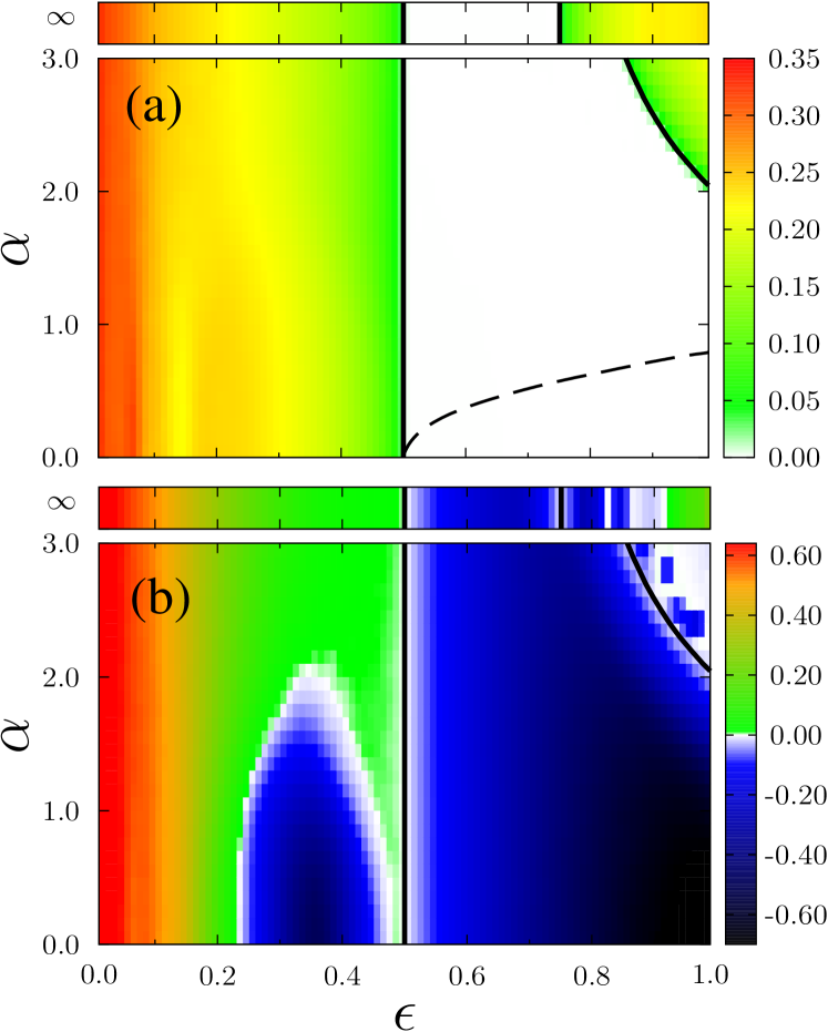
Figure 1: (Color online) Asynchronous updating. Phase diagrams, in the parameter plane $\epsilon-\alpha$, showing $\langle\sigma\rangle$ (a) and $\lambda_{\rm max}$ (b) in color scale. The black solid lines correspond to the theoretical prediction given by Eq.(7). The dashed line, that delimits the region of chaotic CS in the synchronous case A, is given by  Eq. (6). In all cases, the array size is $N=1000$. For each value of $\epsilon$, we used 100 time steps, after $t=10^{4}$ has elapsed, over a typical trajectory, starting from random initial configurations where each $x^{i}$ is random in [0,1], to compute $\langle\sigma\rangle$ and $\lambda_{\rm max}$.

The bifurcation diagrams of $h_{t}$, as well as $\langle\sigma\rangle$ and $\lambda_{\rm max}$, vs the coupling strength $\epsilon$ are shown in Fig. 2, in the extreme cases $\alpha\rightarrow\infty$ (a) and $\alpha=0$ (b). First we notice that even in the case of nearest neighbors ($\alpha\to\infty$), CS can emerge (pointed by intervals of $\epsilon$ where $\langle\sigma\rangle=0$). But, in those regions, the negative $\lambda_{\rm max}$ indicates that, differently from the synchronous case, CS is non-chaotic. In fact, synchronization occurs at $x^{\star}=3/4$, that corresponds to a fixed point of the logistic map, as evinced by the plot of $h_{t}$. Chaos is suppressed in all the CS domain such that the collective state of the system is always the spatially homogeneous one given by $x^{\star}=3/4$. This is the unstable fixed point of the individual map, that gained stability in the coupled system squeeze .

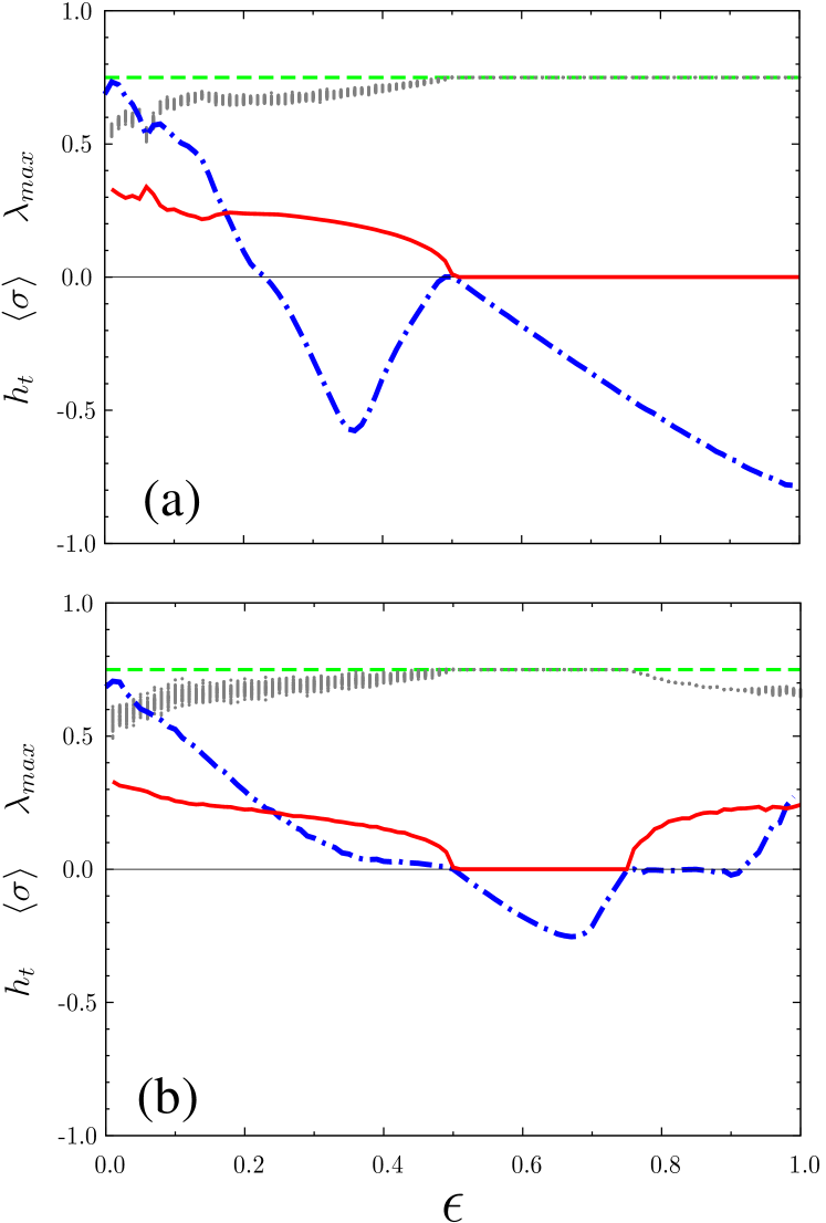
Figure 2: (Color online) Asynchronous updating. Cuts of the phase diagrams in Fig. 1, at $\alpha=\infty$ (a) and $\alpha=0$ (b), showing $\langle\sigma\rangle$ (red solid line), $\lambda_{\rm max}$ (blue dash-dot line) and, additionally, the order parameter $h_{t}$ (light-gray dots), all vs. the coupling $\epsilon$. The green dashed line, in (a) and (b), corresponds to the fixed point at $h_{t}=3/4$, plotted as a reference.

We can derive the critical values of $\epsilon$, under the asynchronous updating, by analyzing first the stability of the fixed point under a synchronous dynamics. In the latter case, the stability condition of a CS solution at a fixed point can be obtained analytically from the eigenvalues $\phi_{k}$, $k=1,\ldots,N$ of the matrix $\mathbf{F}$ defined in Eq. (5). Differently from case A, in the fixed point $x^{\star}=3/4$ where $f^{\prime}(x^{\star})=-2$, $\mathbf{F}$ is time independent. For stability, we must request that $|\phi_{k}|\leq 1$ for $k=1,\ldots,N-1$. Therefore the condition for transverse stability is the same given by Eq. (6). However, this stability is transversal, while, in case A, $x^{\star}=3/4$ is unstable along the synchronization subspace, therefore the dynamics becomes chaotic, as seen in the previous subsection. In the asynchronous case, the scenario is rather different, as shown in Fig. 1, and can be heuristically understood as follows unstableFP1 . Near the lower frontier $\epsilon_{c}$, where the eigenvalues are close to -1, and therefore the individual deviations from the fixed point change sign at each iteration, the nonlocal contribution is expected to cancel out. Therefore, the stability condition that the eigenvalues must fulfill becomes $-1\leq-2(1-\epsilon)$, implying $\epsilon_{c}=1/2$ for all $\alpha$. Differently, in the upper frontier $\epsilon_{c}^{\prime}$, such cancellation does not take place, then the inequality (6) for $\epsilon_{c}^{\prime}$ in the synchronous case must still hold. Therefore,

$$1/2=\epsilon_{c}\leq\epsilon\leq\epsilon_{c}^{\prime}=3/\left(2(1-{\rm min}[\{a_{k}\}])\right),$$ (7)

which is in excellent accord with numerical outcomes, as can be seen in Fig. 1.a.

III.3 Delayed dynamics

Now we consider the following time-delayed CML

$$x_{t+1}^{i}=(1-\epsilon)f(x_{t}^{i})+\epsilon\sum_{r=1}^{N^{\prime}}A(r)\Bigl{(}f(x_{t-\tau_{i,i-r}}^{i-r})+f(x_{t-\tau_{i,i+r}}^{i+r})\Bigr{)},$$ (8)

where the whole number $\tau_{i,j}$ is the delay of element $i$ in response to element $j$. The updating of the set of maps is performed simultaneously.

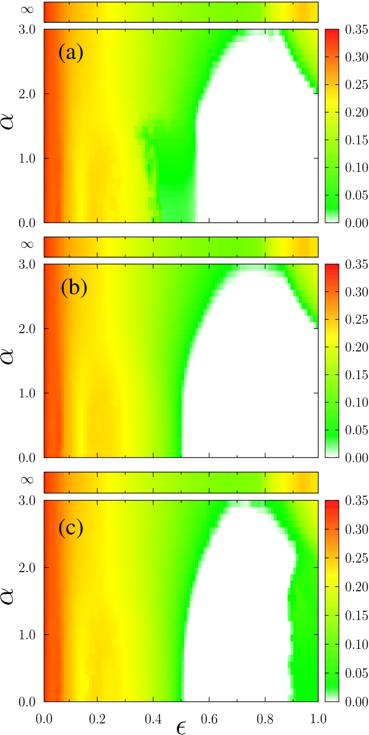
Figure 3: (Color online) Time-delayed dynamics. Phase diagrams, in the parameter plane $\epsilon-\alpha$, showing $\langle\sigma\rangle$ in color scale, for the binary distribution ($\tau=1,0$, with probabilities $p$, $1-p$), with $p=0.45$ (a), $p=0.5$ (b) and $p=0.55$ (c). White regions indicate CS states, where $\langle\sigma\rangle=0$.

We analyzed different distributions of delays, where $\tau_{ij}$ can be fixed or randomly chosen at each time $t$ with a given probability distribution. We report below the cases that we found better match with the asynchronous case B.

First, we consider a binary distribution where $\tau$ can take solely the values 1 and 0, with probabilities $p$ and $1-p$, respectively. Hence $p=0$ recovers the synchronous case A, while $p=1$ corresponds to a dynamics with fixed delay $\tau=1$.

Phase diagrams of $\langle\sigma\rangle$ for values of $p\approx 0.5$ are shown in Fig. 3. For $0\leq\alpha\lesssim 1$ the portraits shown in Figs. 1.a and 3.b ($p=0.5$) are equivalent, in the sense that the intervals of $\epsilon$ for non-chaotic CS are coincident. In fact, the case that better approaches the asynchronous updating scenario B is provided by $p=0.5$ (see Fig. 3), which yields the largest domain of CS in the plane $\epsilon-\alpha$. Furthermore, like in case B, the chaotic dynamics is suppressed with CS occurring at $x^{\star}=3/4$. However, for $\alpha>1$, differently to the asynchronous case where $\epsilon_{c}$ remains constant (Fig. 1.a), now $\epsilon_{c}$ increases with $\alpha$ (Fig. 3.b). As a consequence, the CS domain shrinks and collapses at $\alpha\simeq 3$. Then, for $\alpha\gtrsim 3$, CS never occurs in the binary delayed case. That is, the equivalence of CS domains for the delayed and asynchronous dynamics fails for short-range couplings. In fact, while long-range couplings favor homogenization, through spatial averaging, short-range couplings promote the formation of spatial domains of synchronized and non-synchronized regions. These spatial patterns are persistent, hindering CS. Some sort of temporal average might compensate the lack of spatial homogenization, through the interplay between temporal and spatial dimensions. However, binary delays do not perform well that task when short-range interactions are involved. We also tested other (non binary) distributions of discrete delays, without finding improvements in the sense of mimicking the asynchronous dynamics.

If the asynchronous updating can be thought as a sort of delayed dynamics, as far as a distribution of non-integer delays is behind, integer values of $\tau_{ij}$ fail in providing equivalence of CS when the range of the interactions is too short. A question is whether that in-equivalence arises due to the discrete nature of time delays. Since the states are accessible at discrete times only, a way to emulate continuous time delays in the real interval $[0,1]$ is by interpolation between the states at $\tau=0$ and $\tau=1$, as if the trajectory were continuous by parts. Namely, we consider the intermediate state

$$\hat{x}_{t}=\beta x_{t-1}+(1-\beta)x_{t-0}\,,$$ (9)

where $\beta$ controls the interpolation point and can take fixed or distributed values. We introduced this prescription into Eq. (8), which becomes

$$x_{t+1}^{i}=(1-\epsilon)f(x_{t}^{i})+\epsilon\sum_{r=1}^{N^{\prime}}A(r)\Bigl{(}f(\hat{x}_{t}^{i-r})+f(\hat{x}_{t}^{i+r})\Bigr{)}.$$ (10)

We observed that when $\beta$ is uniformly distributed in [0,1], the critical frontier is closer to the asynchronous one than in the case of binary delays (not shown), but the similarity is enhanced when the distribution concentrates around the middle point and the coincidence is perfect when $\beta=1/2$, as depicted in Fig. 4, where we consider different values of $\beta\simeq 0.5$. We remark that outside the CS domain, differential features emerge, as can be seen by comparing the color maps in Figs. 1.a and  4.b, with more complex structures in the delayed system. That is, the equivalence holds only for the CS domain when $\beta=0.5$.

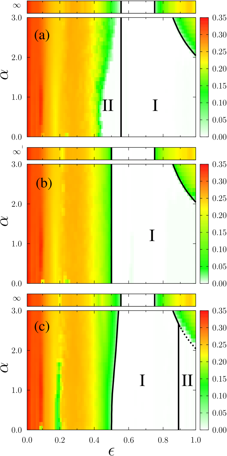
Figure 4: (Color online) Time-delayed dynamics. Phase diagrams, in the parameter plane $\epsilon-\alpha$, showing $\langle\sigma\rangle$ in color scale for different values of $\beta$ of the pseudo continuous dynamics ($\hat{x}_{t}=\beta x_{t-1}+(1-\beta)x_{t-0}$): $\beta=0.45$ (a), $\beta=0.5$ (b) and $\beta=0.55$ (c). White regions indicate CS states, where $\langle\sigma\rangle=0$. The thick lines were obtained analytically through the stability condition $|\lambda|\leq 1$, where $\lambda$ are the eigenvalues of $\mathbf{\tilde{F}}$ defined by Eq. (11), as explained in the text. They delimit the region where the CS state is a fixed point ($x^{\star}=3/4$, subdomain “I”). While the subdomain “II” corresponds to regular CS states of period larger than 1.

The CS frontier for the system described by Eq. (10) can be analytically determined as follows. First we cast the CML (10) in Markovian form by the usual procedure of extending the phase space, such that $\mathbf{\delta\tilde{x}}_{t}=(\mathbf{\delta x}_{t},\mathbf{\delta x}_{t-1})$. As a consequence, the matrix $\mathbf{\tilde{F}}$ which rules the linearized evolution around the fixed point, $\mathbf{\delta\tilde{x}}_{t}=\mathbf{\tilde{F}}\mathbf{\delta\tilde{x}}_{t-1}$, is the block matrix

$$\mathbf{\tilde{F}}=\left(\begin{array}[]{c|c}[(1-\epsilon)\mathbb{1}+(1-\beta)\epsilon\mathbf{A}]f^{\prime}&\beta\epsilon\mathbf{A}f^{\prime}\\ \hline\cr\mathbb{1}&\mathbb{0}\end{array}\right),$$ (11)

where $f^{\prime}\equiv f^{\prime}(x*)=f^{\prime}(3/4)=-2$. By setting $\mathbf{\tilde{F}}(u,v)^{t}=\lambda(u,v)^{t}$, and substituting Eq. (11), it can be easily shown that the eigenvalues $\lambda$ of the block matrix are related to the eigenvalues of $\mathbf{A}$, through the characteristic equation

$$\lambda^{2}+2\lambda[1-\epsilon+\epsilon(1-\beta)a_{k}]+2\beta\epsilon a_{k}=0.$$ (12)

(Notice that, since this is a second order polynomial, two values of $\lambda$ arise for each value $a_{k}$.) Of course, if $\beta=0$, then the eigenvalues of $\mathbf{F}$ are recovered. The condition $|\lambda|\leq 1$ for all the eigenvalues furnishes the region of stability of the fixed point. For $\beta=1/2$, the frontier of the asynchronous case is exactly recovered, as can be seen in Fig. 4b. The eigenvalues $\lambda$ associated to the largest eigenvalue of $\mathbf{A}$, $a_{N}=1$, provide the longitudinal stability, while the remaining ones furnish the transverse stability.

In Fig. 4a-c, the white region corresponds to CS states ($\langle\sigma\rangle=0$). Inside that region, the CS state is a fixed point ($x^{\star}=3/4$) in subdomain “I”, while the subdomain “II” corresponds to regular CS states of period larger than 1. Frontiers of the region where CS occurs at the fixed point are given by transverse stability condition, except those borders separating regions I and II, in panels (Fig. 4.a and  4.c), which are given by the longitudinal stability condition, $1/4\leq\beta\epsilon\leq 1/2$. If $\beta=0$, the fixed point cannot be stable for any coupling strength $\epsilon$, but above $\beta=1/2$, there emerges an interval of values of $\epsilon$ for which the fixed point becomes stable. This explains the emergence of the stability of the locally unstable fixed point.

IV Final remarks

We found that binary discrete delays manage to mimic CS observed in asynchronous dynamics, but this occurs only if the interactions are sufficiently non-local. In contrast, pseudo-continuous delays reproduce exactly the asynchronous CS states, independently of the range of the interactions. This equivalence allows to embrace, in a unified frame, delayed and asynchronous dynamics, usually treated separately. The asynchronous case is usually analyzed heuristically, due to the mathematical difficulties involved, while there are analytical procedures to treat the delayed dynamics (by extending the phase space to turn the system Markovian). In this context, our finding provides an alternative way to determine the CS domains for an asynchronous update through a delayed one.

As side results, the outcomes put into evidence the interplay between the spatial and temporal dimensions in pattern formation, and also have implications in control of chaos, as far as we found a time delayed scheme more efficient than discrete delays in the stabilization of a locally unstable state, which can be understood along the lines discussed at the end of Sec. III.3.

Despite we used a particular CML in numerical examples, the analytical considerations apply to a general class of CMLs, following the form given by Eq. (1), with generic $A(r)$, and a chaotic unimodal map as local dynamics. However, the results might apply to a larger class of CMLs, e.g., including advective lind04b coupling or bistable local dynamics lind04c .

Acknowledgments: We acknowledge Brazilian agencies CNPq and FAPERJ for financial support.

References

- (1) A. Pikovsky, M. Rosenblum, J. Kurths, Synchronization: a universal concept in nonlinear sciences, The Cambridge nonlinear science series (Cambridge University Press, Cambridge,2001).
- (2) S.C. Manrubia, A.S. Mikhailov, and D. Zanette, Emergence of Dynamical Order. Synchronization Phenomena in Complex Systems (World Scientific, Singapore, 2004).
- (3) Y. Kuramoto, Chemical Oscillations, Waves, and Turbulence (Springer, Berlin, 1984).
- (4) J. Crutchfield, K. Kaneko, Theory and Applications of Coupled Map Lattices (World Scientific, Singapore, 1987).
- (5) J. Hertz, A. Krogh, R. G. Palmer, Introduction to the Theory of Neural Computation (Addison-Wesley, Redwood, 1991).
- (6) M.D. Shrimali, S. Sinha, K. Aihara, Phys. Rev. E 76, 046212 (2007).
- (7) M. Mehta, S. Sinha, Chaos 10, 350 (2000).
- (8) E. D. Lumer, G. Nicolis, Physica D 71, 440 (1994).
- (9) N. Crokidakis, V. H. Blanco, C. Anteneodo, Phys. Rev. E 89, 013310 (2014).
- (10) N. Crokidakis and C. Anteneodo, Phys. Rev. E 86, 061127 (2012).
- (11) H. Atmanspacher, T. Filk, H. Scheingraber, Eur. Phys. J. B 44, 229 (2005).
- (12) H. Atmanspacher, H. Scheingraber, I. J. Bifurcation and Chaos 15, 1665 (2005).
- (13) C. Masoller, A.C. Martí, Phys. Rev. Lett. 94, 134102 (2005).
- (14) M. Ponce C., C. Masoller, A. C. Martí, Eur. Phys. J. B 67, 83 (2009).
- (15) A. C. Martí, M. Ponce, C. Masoller, Phys. Rev. E 72, 066217 (2005).
- (16) Theme Issue ’Delayed complex systems’, Phil. Trans. Royal Soc. A, compiled and edited by W. Just, A. Pelster, M. Schanz and E. Schöll (2009).
- (17) Y. Kuramoto, H. Nakao, Physica D 103, 294 (1997).
- (18) C.Anteneodo, A. Batista, R. Viana, Phys. Lett. A 326, 227 (2004).
- (19) C.Anteneodo, A. Batista, R. Viana, Physica D 223, 270 (2006).
- (20) P. G. Lind, J. Corte-Real, J. A. C. Gallas, Phys. Rev. E 69, 026209 (2004).
- (21) C. Anteneodo, C. Tsallis, Phys. Rev. Lett. 80, 5313 (1998).
- (22) F. Tamarit, C. Anteneodo Phys. Rev. Lett. 84, 208 (2000).
- (23) P.G. Lind, J.A.C. Gallas, H.J. Herrmann, Phys. Rev. E 70, 056207 (2004).
- (24) J. P. Eckmann, D. Ruelle, Rev. Mod. Phys. 57 617 (1985).
- (25) G. Benettin, L. Galgani, A. Giorgilli, and J.-M. Strelcyn, Meccanica 15, 9 (1980); ibid. 21 (1980).
- (26) P.G. Lind, J. Corte-Real, J.A.C. Gallas, Phys. Rev. E 69, 066206 (2004).
- (27) P.G. Lind, S. Titz, T. Kuhlbrodt, J.A.M. Corte-Real, J. Kurths, J.A.C. Gallas, U. Feudel, Int. J. Bif. and Chaos 14, 999 (2004).