Do investors trade too much?
A laboratory experiment

Abstract

We run experimental asset markets to investigate the emergence of excess trading and the occurrence of synchronised trading activity leading to crashes in the artificial markets. The market environment favours early investment in the risky asset and no posterior trading, i.e. a buy-and-hold strategy with a most probable return of over $600\%$. We observe that subjects trade too much, and due to the market impact that we explicitly implement, this is detrimental to their wealth. The asset market experiment was followed by risk aversion measurement. We find that preference for risk systematically leads to higher activity rates (and lower final wealth). We also measure subjects’ expectations of future prices and find that their actions are fully consistent with their expectations. In particular, trading subjects try to beat the market and make profits by playing a buy low, sell high strategy. Finally, we have not detected any major market crash driven by collective panic modes, but rather a weaker but significant tendency of traders to synchronise their entry and exit points in the market.

JEL codes: C91, C92, D84, G11, G12.

Keywords: Experimental Asset Markets, Trading Volumes, Crashes, Expectations, Risk Attitude.

Acknowledgments: This work was partially financed by the EU “CRISIS” project (grant number: FP7-ICT-2011-7-288501-CRISIS), Fundação para a Ciência e Tecnologia, and the Ministry of Education, Universities and Research of Italy (MIUR), program SIR (grant n. RBSI144KWH).

1 Introduction

Financial bubbles and crises are potent reminders of how far investors’ behaviour may deviate from perfect rationality. Many behavioural biases of individual investors are now well documented, such as the propensity for trend following or extrapolative expectations (Greenwood and Shleifer,, 2014), herding behavior (Cipriani and Guarino,, 2014), disposition effect (Grinblatt and Keloharju,, 2001), home bias (Solnik and Zuo,, 2012), over and underreaction to news (Barber and Odean,, 2008); see Barberis and Thaler, (2003) and Barber and Odean, (2013) for comprehensive overviews.

A well established fact about individual trading behaviour which is in stark contrast with the predictions of rational models is the tendency of individual investors to trade too much (Odean,, 1999). Many investors trade actively, speculatively, and to their detriment. Odean, (1999), Barber and Odean, (2000), Odean and Barber, (2011) and Barber et al., (2009) among others show that the average return of individual investors is well below the return of standard benchmarks and that the more active traders usually perform worse on average. In other words, these investors would do a lot better if they traded less. Moreover, as noted in Barber and Odean, (2013), individual investors make systematic, not random, buying and selling decisions.

Based on the empirical evidence mentioned above, the goal of this paper is to study the emergence of excess trading in an experimental financial market where trading is clearly detrimental for investors’ wealth. We aim to gain a deeper understanding not only of why agents trade, but also how correlated is their activity. In particular, we want to study whether synchronisation of trading activity leads to unstable market behaviour, such as crashes driven by panic, herding and cascade effects.

Market laboratory experiments now have a rather long history. The most influential paradigm for multi-period laboratory asset markets was developed in Smith et al., (1988). The asset traded in their experiment has a known finite life span and pays a stochastic dividend at the end of each period. The fundamental value of the asset falls deterministically over time, and lacking a terminal value the asset expires worthless. A salient result is that asset prices in the experimental markets follow a “bubble and crash” pattern which is similar to speculative bubbles observed in real world markets. This seminal work has spawned a large number of replications and follow-ups, see Palan, (2013) for an extensive overview.

The present study belongs to the above tradition of experimental markets but implements a different market mechanism. Instead of trading in a continuous double auction, subjects can submit buying and selling orders, executed by a market maker, for a fictitious asset that increases in value at a known average rate and has an indefinite horizon.

One particularly interesting feature of our laboratory market is that we model and implement price impact, i.e. the fact that the very action of agents modifies the price trajectory. This is now believed to be a crucial aspect of real financial markets, which may lead to feedback loops and market instabilities (Bouchaud et al.,, 2009; Cont and Wagalath,, 2014; Caccioli et al.,, 2014; Lillo et al.,, 2003; Lillo and Farmer,, 2004). What is of particular interest in our experiment is that excess trading significantly impacts the price trajectory and is strongly detrimental to the wealth of our economic agents. In other words, unwarranted individual decisions can lead to a substantial loss of collective welfare, when mediated by the mechanics of financial markets.

One advantage of using a controlled laboratory environment is that it allows us to directly measure individual characteristics and relate them in a systematic way to trading activity. Previous empirical studies show that individual risk attitude could have an impact on trading in asset markets. For example, Robin et al., (2012) and Fellner and Maciejovsky, (2007) find that risk-aversion leads to smaller bubbles and less trade in asset market. Moreover, Keller and Siegrist, (2006) did a mail survey and found that financial risk tolerance is a predictor for the willingness to engage in asset markets. In the light of the aforementioned empirical evidence, we measure subjects’ risk aversion using a standard Holt and Laury, (2002) procedure and link it to individuals’ trading activity.

We also elicit individual price expectations in order to better understand what leads to investors’ decision of engaging actively in trading activity as well as being inactive in the market. Since we collect both data on individual trading decisions as well as price expectations, we are able to give a consistent picture of activity and inactivity as a consequence of price return expectations. See also Smith et al., (1988), Hommes et al., (2005, 2008) and Haruvy et al., (2007) among others for studies on the role of expectations in generating bubbles and crashes in experimental asset markets.

Our findings can be summarised as follows. Although the market environment clearly favours a buy-and-hold strategy (see below), we observe that our subjects engage in excessive trading activity, which is both individually and collectively detrimental, since the negative impact of sellers reduces the price of our artificial asset. When the experiment is immediately repeated with the same subjects, we see a significant improvement of the collective performance, which is however still substantially lower than the (optimal) buy-and-hold strategy.

Moreover, although our subjects are physically separated and cannot communicate, we have seen that a significant amount of synchronisation takes place in the decision process, that can therefore only be mediated by the price trajectory itself. This resonates with what happens in real financial markets, where price changes themselves appear to be interpreted as news, leading to self-reflexivity and potentially unstable feedback loops (see e.g. Bouchaud et al., (2009); Hommes, (2013)). In fact, our experimental setting was such that panic and crashes were possible but this did not happen. Although we observed a significant level of synchronisation, no cascades or “fire sales” effects could be detected for our particular choice of parameters.

Consistently with the empirical evidence mentioned above, we find that risk loving attitudes lead to higher trading activity and this is detrimental to individual wealth.

Finally, subjects seem to have a desire to trade actively, motivated by a willingness to “beat the market”, as revealed by the analysis of individual price expectations. Most subjects engage in trading activity trying to buy low and sell high, while the decisions of being inactive and hold cash (shares) depends on whether they expect price returns lower (higher) than average.

The outline of this paper is as follows. Section 2 describes the experimental motivation and set-up. The precise instructions given to our subjects are detailed in Appendix C. Section 3 explains the theoretical benchmark to which we want to compare the experimental results. In particular, we show that (risk-neutral) rational agents should favour, in the present market setting, a buy-and-hold strategy. We then summarize our main results in Section 4, which includes a refined statistical analysis of agents’ trading activity in Section 4.1. In Section 4.2 we relate individual risk attitude to activity rate and final wealth, while in Section 4.3 we link price forecasts and trading behaviour. Section 5 offers our conclusions, open questions, and future experiments.

2 Experimental Design

The basic idea of our experiment is to propose to subjects a simple investment “game” where they can use the cash they are given at the beginning of the experiment to invest in a fictitious asset that will – they are told – increase in value at an average rate of $m=2\%$ per period. The asset “lives” for an indefinite horizon, i.e. the game may stop randomly at each time step with probability $p=0.01$. The game is thus expected to last around $100$ time steps. Subjects are also informed that random shocks impact the price of the asset in each period. In the absence of trade, price dynamics are described by

$$p_{t+1}=p_{t}\cdot\exp(m+s\eta_{t}),$$ (1)

where $m=2\%$, $\eta_{t}$ is a noise term drawn from a Student’s t-distribution with 3 degrees of freedom and unit variance, as commonly observed in financial markets (Gopikrishnan et al.,, 1998; Jondeau and Rockinger,, 2003; Bouchaud and Potters,, 2003), and $s$ is a constant that sets the actual amplitude of the noisy contribution to the evolution of the price (i.e. the price volatility) and is chosen to be $s=10\%$. These numbers correspond roughly to the average return and the volatility of a stock index over a quarter. Therefore, in terms of returns and volatility, one time step in our experiment roughly corresponds to three months in a real market, and 100 steps to 25 years.

If an amount $w_{0}$ is invested in the asset at time $t=0$, the wealth of the inactive investor will accrue to

$$w_{T}=w_{0}\exp\left[mT+\xi s\sqrt{T}\right]$$ (2)

at time $T$, where the second term of the exponential implies random fluctuations of root mean square (RMS) $s$ per period with $\xi$ defined as a noise term with zero mean and unit variance. The numerical value of the term in the exponential is therefore equal to $2\pm\xi$ for $T=100$, leading to a substantial most probable profit of $e^{2}-1\approx 640\%$. As we shall show below, the fully rational decision in the presence of risk-neutral agents is to buy and hold the asset until the game ends; for the students participating in the experiment, the most probable gain would represent roughly $\text{EUR }160$, a very significant reward for spending two hours in the lab. In other words, the financial motivation to “do the right thing” is voluntarily strong.

In order to make the experiment more interesting, and trading even more unfavourable, the asset price trajectory is made to react to the subjects decisions, in a way that mimics market impact in real financial markets. The idea is that while a buying trade pushes the price up, a selling trade pushes the price down (for a short review on price impact, see e.g. Bouchaud, (2010)). As an agent submits a (large) buying or selling order at time $t$, the price $p_{t+1}$ at which the transaction is going to be fully executed is (a) not known to him at time $t$ and (b) adversely impacted by the very order that is executed. It is made very clear to the subjects that their transaction orders will be executed at the impacted price, meaning that the impact will amount for them as a cost. This should therefore be a strong incentive not to trade.

The price updating rule described in Eq. (1) is easily modified to include price impact and now reads

$$p_{t+1}=p_{t}\cdot\mathrm{exp}\left(m+s\eta_{t}+I_{t}\right).$$ (3)

The term $I_{t}$ is the price impact caused by all the orders submitted at time $t$, which we model as:

$$I_{t}=\frac{N_{t}}{N}\frac{B_{t}-S_{t}}{B_{t}+S_{t}},$$ (4)

where $N_{t}$ is the number of subjects who submitted an order at time $t$ and $N$ is the total number of subjects in a given market session (i.e. the “depth” of our market). $B_{t}$ and $S_{t}$, in currency units, are the total amount of buying orders and selling orders, respectively. Note that for a single buying (or selling) order, the impact is given by $1/N$, i.e. around $3\%$ for a market with 30 participants (and less if the market involved more participants, as is reasonable). On the other hand, if all the agents decide to buy (or sell) simultaneously, the ensuing impact factor would be $100\%$.

With the introduction of market impact, subjects have to guess if the observed price fluctuations are due to “natural” fluctuations, i.e. to the noise term they are warned about at the beginning of the game, or if they are due to the action of their fellow subjects. This was meant to provide a potentially destabilizing channel, where mild sell-offs could spiral into panic and crashes.

We are therefore interested in studying whether excess trading emerges in a market environment which clearly penalises trading, and whether synchronisation of trading activity, such as avalanches of selling orders triggered by panic, results in big market crashes.

2.1 Implementation

The experiment was programmed in Java using the PET software and it was conducted at the CREED laboratory at the University of Amsterdam in May 2014. In the beginning of the experiment each subject is randomly assigned a computer in the laboratory and physical barriers guarantee that there is no communication between subjects during the experiment. The experiment was conducted with 201 subjects, divided in 9 experimental markets with a median number of participants per market of 24 subjects. The experiment lasted about two hours and before starting the experiment subjects had to answer a final quiz to make sure they understood the rules of the game (see Appendix C).

At the beginning of the experiment each subject is endowed with 100 francs. Each period lasts 20 seconds, during which subjects have to decide whether they want to hold cash or shares in the next period. If subjects did not make any decision within the limit of 20 seconds, their current market position would simply carry over to the next period. If they have cash at period $t$, they can decide either to use it all to buy shares or to stay out of the market at period $t+1$. Conversely, if they have shares at period $t$, they have to choose between selling them all for cash or staying in the market at period $t+1$. Fractional orders are not allowed, therefore each player is either in the market or out of the market at all times.

In order to avoid possible “demand effects”, i.e. trading volumes in the markets related to the fact that participation in the asset market is the only activity available for subjects (Lei et al.,, 2001), we introduce a forecasting game in which subjects are asked to forecast the asset price and rewarded according to the precision of their forecast.

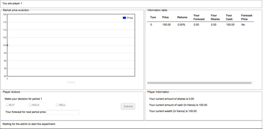
The information visualised on subjects’ screens include a chart displaying the asset price evolution together with a table reporting time series of asset prices, returns, individual holdings of cash and shares and price forecasts. Fig. 18 in Appendix A shows a screenshot of the experiment.

In order to mitigate behaviour bias towards the end of the experiment, we implement an indefinite horizon (see Crockett and Duffy, (2013) for an example in artificial asset markets). In each period of the experiment there is a known constant continuation probability $1-p=0.99$. Moreover, each subject participates in two consecutive market sessions, after a short initial practice session to familiarise with the software, so that learning mechanisms can be studied.

When a market session is terminated, subjects’ final wealth is defined as follows: if they are holding cash, their amounts of francs will determine their wealth; if they are holding shares, their wealth is defined as the market value of their shares, i.e. their amounts of shares times the market price at the end of the sequence. In fact, at the end of the market sequence shares are liquidated at the market price without any price impact. At the end of the experiment subjects’ net market earnings are computed as their end-of-sequence balance minus their initial endowment. At the end of the experiment, each subject rolls a dice to determine which of the two market sessions will be used to calculate his take-home profits (which also include the earnings from the forecasting game). The exchange rate is 100 francs to EUR 25.

Finally, we asked subjects to participate in a second experiment involving the Holt and Laury, (2002) paired lottery choice instrument. This second experiment occurred after the asset market experiment had concluded and was not announced in advance, to minimize any influence on decisions in the asset market experiment.

The complete experimental instructions can be found in Appendix C.

3 Theoretical Benchmark

In this section we devote attention to the theoretical rational benchmark for this experiment and derive the equilibrium of the game under the assumption of full rationality and common knowledge of rationality. It is worth remarking at this point that this experiment is a de facto risk-free opportunity, in the sense that the subjects are paid at the end of the experiment if their net profit is positive but do not owe any amount if their net profit ends up negative.

3.1 Risk neutrality

Let the wealth of the agent be $w_{t}$ at time $t$. If we assume that the session ends at $t=t_{F}$, fully rational agents have two possible strategies. The first one is to stay out of the market for $t>1$ and hold cash until $t=t_{F}$ which yields an expected final wealth $\mathbb{E}\left(w_{t_{F}}\right)=w_{0}$.

The second strategy consists in being fully invested in the market at $t=1$ and hold the shares until $t=t_{F}$. In fact, in every period holding shares is an equilibrium of the stage game since the strategy “Hold” is the best response to any number of players $n$ that an agent might expect to sell. This strategy yields $\mathbb{E}\left(w_{t_{F}}\right)\approx w_{0}\cdot(1+m+s^{2}/2)^{t_{F}}$ regardless of the initial condition. The average outcome of the first strategy is at best zero profit (remember that subjects only keep net profits), while the second strategy provides large expected profits when the experiment session lasts for a long time.

Therefore the rational benchmark, with a risk neutral population, is to get in the market at $t=1$ and hold the shares until the end of the experiment. The longer the duration of the experiment, the larger the expected profits.

3.2 Myopic risk aversion

Empirical evidence suggests that risk attitude affects trading behaviour. In the following we consider the case of risk averse traders using the utility function proposed by Holt and Laury, (2002)

$$U(w)=\frac{1-\exp\left(-\alpha w^{1-r}\right)}{\alpha},$$ (5)

where $\alpha$ and $r$ are positive parameters. Based on the fact that the utility function in Eq. (5) is concave, one could be tempted to consider that for high enough volatility $s$, myopic rational traders, i.e. traders who only look one time step ahead when making their decisions, would choose to step out of the market as soon as their wealth reached a certain level. However, this is not the case because if they decided to sell, the price of the asset would not only be negatively affected by their action through the impact factor $I_{t}$, but also be impacted by the noise $s\eta_{t}$. This is due to the fact that transactions ordered at time $t$ are executed at the price realized in $t+1$, meaning that agents deciding to step out of the market at time $t$ are still subject to price volatility. Consequently, it is clear that, for a given time step, it is always a better option to stay in the market and be affected by the noise factor alone, instead of selling and being affected by both the noise factor and the negative impact factor.

Using Eq. (5) we can also study a few cases of bounded rationality within myopic optimisation. In particular we compare, for different levels of wealth, the expected utility given by Eq. (5) in the following anticipated scenarios: all players hold to their shares, taking into account the volatility of the noise term ($I=0$); all players sell their shares, taking into account the volatility of the noise term ($I=-1$); all players sell their shares, without taking into account the volatility of the noise term ($I=-1$ no noise); one player only sells his shares, without taking into account the volatility of the noise term ($I=-0.01$ no noise).

These scenarios are compared in Fig. 1 below. The magnitude of the noise $s$ defines most of the differences.

(a) RMS $s=0.1$

(b) RMS $s=1.0$

Figure 1: Expected utility in Eq. (5) for different scenarios with bounded rationality, volatility $s=0.1$ (left) and $s=1.0$ (right) and varying level of net wealth $W(t)$. The coloured regions correspond to 1-$\sigma$ around the average utility.

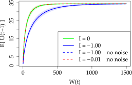
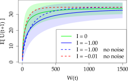
Fig. 1 gives insight on the possible behaviour of risk-averse players. Comparing the solid lines we confirm the intuition presented above: these solid lines never intersect and it is always better for all agents to stay in the market (green solid line) than to step out collectively (blue solid line). However, when we consider bounded rationality and myopic risk-averse traders, the conclusion may be different, in particular when the random fluctuations of the market, which impact the price at each time step, are not taken into account. Consider for example the utilities, computed without taking into account the random fluctuations, for the cases in which only one agent sells (red dashed line) and everyone sells (blue dashed line), and compare them with the case in which everyone stays in the market (green solid line). In these scenarios, there will be a value of wealth $W(t)$ above which, in the mind of these boundedly rational agents, it pays off to sell whatever they are holding. This point depends on the agent thinking either that he will be the only one selling or that everyone will, as well as on the magnitude of the random fluctuations or noise $s$. These values are critical thresholds which we represent as a function of $s$ in Fig. 2 through numerical simulations.

Figure 2: Critical threshold values $W^{*}$, as a function of $s$, beyond which the single-player-out (in red) and all-out strategies (in black) are triggered (corresponding, respectively, to the intersection point of the green/red dotted lines and green/blue dotted lines in Fig. 1).

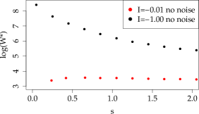
As we would expect from the concavity of the utility function in Eq. (5), the value $W^{*}$ beyond which boundedly rational agents of this sort would sell decreases as a function of $s$ when they consider the possibility of everyone selling at the same time.

In the presence of myopic boundedly rational agents of the sort considered in the section, heterogeneity in risk preferences would lead to threshold strategies in which traders, when wealth increases beyond a critical value $W^{*}$, get nervous and get out of the market. This scenario does not, however, account for the variability amongst agents, which most certainly impacts observed events in real markets and, as we shall see below, the trading activity observed in our experiment.

4 Experimental Results

4.1 Trading activity

In this section we report on the trading activity observed in the experiment. Subsection 4.1.1 describes results on the volume of trading activity in relation to subjects’ wealth. Subsection 4.1.2 studies synchronization in subjects’ trading activity, while Subsection 4.1.3 investigates the presence of common patterns in subjects’ trading behaviour.

4.1.1 Excess trading and wealth

It is clear that if all subjects adopted the strategy of buying and holding the shares until the end of the game, the price impact would be $I(t)\equiv 0$ and the realized price at the end of the market sequence would lead to a most probable $640\%$ increase in wealth. What we observe instead is that subjects keep on trading in and out of the market. The trading activity is in fact so high in the first market sessions that they barely break even, earning a meagre $0.75\%$ on average. Remarkably, all groups learn to some extent and trade much less in the second market sessions, leading to a much higher average earning of $92\%$. These results are somewhat in line with findings in the literature on experimental asset markets showing that sufficient experience with an asset in certain environments eliminates mispricing and the emergence of bubbles (Smith et al.,, 1988; King,, 1991; Van Boening et al.,, 1993; Dufwenberg et al.,, 2005; Haruvy et al.,, 2007; Lei and Vesely,, 2009). In fact we observe, as a result of learning, consistently different behaviour of subjects in the second market sequences when compared to their behaviour in the first sequences. The Welch two-sample t-test applied to the final wealth and average activity rate of each subject in first and second runs statistically confirms this difference ($\text{p-value}\approx 2^{-16}$). Therefore in the following analysis we merge all first market sessions into one dataset and all second sessions into another dataset. These aggregated data sets lead to the price time series illustrated in Fig. 3.

(a) First sessions: quantities averaged over 198 subjects (18 for the last point). The correlation between realized price log returns and price log returns in the absence of trading is $0.85$.

(b) Second sessions; quantities averaged over 201 subjects (23 for the last point). The correlation between realized price log returns and price log returns in the absence of trading is $0.89$.

Figure 3: Average price time series for first and second market sessions.

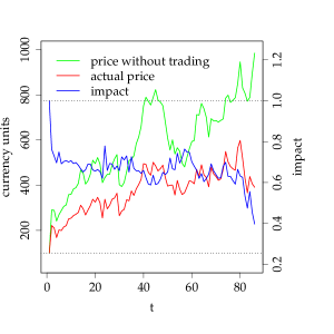
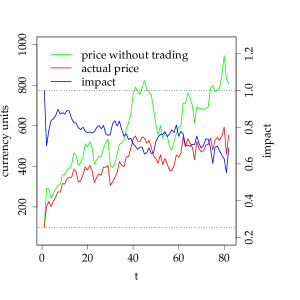
We remark that the durations of the sessions were all different because of the indefinite time horizon. Thus, the number of data points used in the averaging process is not the same for each time $t$ but a decreasing step function of $t$ (this is clearly visualised in Fig. 4 below).

The lines in green represent the “bare” price time series, i.e. the price evolution that would have occurred in the market if all agents had played the buy-and-hold strategy. A comparison with the red lines, depicting the realized prices, immediately reveals that trading significantly weakens the upwards price trend via the impact factor (blue lines): the average slope (i.e. price trend) is divided by a factor of approximately $2$ in the first sessions and $1.5$ in the second sessions. The realized prices in Fig. 3 are proxies for the maximum earnings a subject would achieve if he used the buy-and-hold strategy within his group. However, the realized price log-returns remain highly correlated with the “bare” price time series: the correlation coefficient is $0.85$ in first market sessions and $0.89$ in second market sessions. The higher values of the slope (i.e. price trend) and of the correlation coefficient for the second sessions are due to a lower trading activity.

Fig. 4 displays the positions of the traders – in the market (green) or out of the market (red) – throughout the experimental market sequences.

(a) First sessions: 198 subjects.

(b) Second sessions: 201 subjects.

Figure 4: Traders’ positions – in the market (green) or out of the market (red) – in first sessions (above) and in second sessions (below).

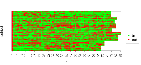
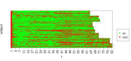
Notice that not all the sessions lasted the same number of periods, hence the white space in both Figs. 4a and Fig. 4b for large $t$. In fact, for each case, only one session – the longest – lasted until the maximum time $t$ displayed, $t=86$ for first sessions (Fig. 4a) and $t=82$ for second sessions (Fig. 4b).

Subjects’ positions – in (holding shares) or out of the market (holding cash) – are mostly intermittent, which implies excessive trading. However, comparing Figs. 4a and 4b, we observe that when the same subjects play for a second time, some of them actually learn the optimal strategy, which translates into “green corridors” in Fig. 4b.

Fig. 5 shows that the distribution of average trading activity changes when the same set of people play the game for the second time, and relates it to agents’ final wealth.

(a) First sessions: 198 subjects and 69-85 periods. The average final wealth was $100.75$ units of currency, the average activity rate $29\%$ and the correlation between the two $-0.62\%$.

(b) Second sessions: 201 subjects and 63-81 periods. The average final wealth was $191.97$ units of currency, the average activity rate $12\%$ and the correlation between the two $-0.73\%$.

Figure 5: Activity rate and final wealth in first sessions (left) and in second sessions (right).

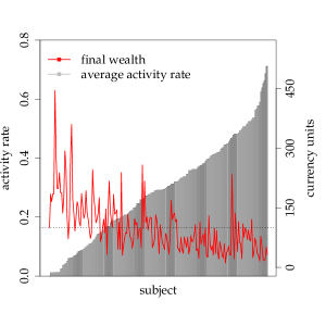
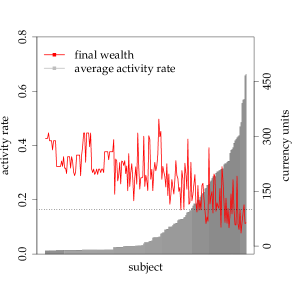
The number of people who keep trading to a minimum increases significantly in second sessions, where only a few outliers keep trading activity above $40\%$, i.e. they changed their market positions in more than $40\%$ of the periods. In both cases, the final wealth of the agents is strongly anti-correlated with average trading activity, which is expected since trading is costly. In fact, if a trader decides to buy shares at period $t$ and to sell them at period $t+1$, he will, on average, end up with less cash than he started because of his own contribution to price impact.

The average wealth of the subjects in first and second sessions is shown in Fig. 6 as a function of time, while Fig. 7 shows the average components of wealth over time.

(a) First sessions, 198-18 subjects.

(b) Second sessions, 201-23 subjects.

Figure 6: Average wealth for first sessions (left) and second sessions (right).

(a) First sessions, 198-18 subjects.

(b) Second sessions, 201-23 subjects.

Figure 7: Average wealth $\overline{W_{t}}$ (black), average cash $\overline{C_{t}}$ (green) and average number of shares $\overline{S_{t}}$ (blue) in first sessions (left) and in second sessions (right).

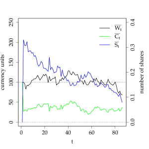
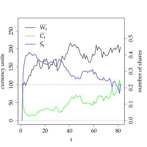
Fig. 6 shows once more that subjects fared much better in second sessions, in which their average final wealth was approximately twice their initial endowment, than in first sessions, in which the vast majority did not even break even. In what concerns the average components of wealth over time, there are also differences between first sessions (Fig. 7a) and second sessions (Fig. 7b). In first sessions, where overall trading activity is high (Fig. 5a), the average wealth does not follow the upward trend one would expect in a set-up with “guaranteed” average growth of $2\%$ per period. In fact, players trade so much that they keep eroding their wealth when they sell and affording fewer and fewer number of shares when they buy. This accounts for a negative impact bias on average and results in very low earnings at the end of the session, as shown in Fig. 6a. On the other hand, in second sessions, where overall trading activity is much lower (Fig. 5b), the average wealth does increase with time. Nevertheless the number of shares owned eventually decreases, which is due not only to excessive trading but also to the fact that some subjects cash in their earnings before the end of the experiment and stay out of the market from that point onwards.

This is particularly visible in Fig. 7b, when a surge in price triggers selling orders over several periods which result in a higher average amount of cash and, naturally, in a lower average number of shares. Although this is also visible in the middle of the time series in first sessions (Fig. 7a), the difference between the two cases is that most of the resulting cash is eventually reinvested in the first sessions, while in the second sessions this does not happen: cash holdings consistently increase after the initial investment phase (Fig. 7b).

As we showed in Sec. 3 the optimal strategy in our experimental set-up would be to collectively buy-and-hold and reap the benefits from the baseline average return of $2\%$ per period in the absence of trading. We see that the behaviour of the agents is very far from this benchmark, even in the second sessions, in spite of a significant decrease in activity. The average performance in second sessions is indeed still far from what it would have been if all subjects used the optimal buy-and-hold strategy, i.e. despite the learning there is still excess trading activity which translates into detriment of collective welfare – since even the “virtuous” agents are adversely impacted by the trading activity of excessively “active” agents.

4.1.2 Collective trading modes – activity correlations, panic & euphoria

Our subjects trade too much, but can we describe in more detail how correlated their activity is? In fact, our initial intuition – that turned out to be quite far from what actually happened — was that the agents would not trade at the beginning of the game, letting the price rise from its initial value of $100$ to quite high values, say $400$ (EUR 100), before starting to worry that others might start selling, pushing the price back down and potentially inducing a panic chain reaction. This would have translated into either a major crash, or perhaps smaller downward corrections, but in any case a significant skewness in the distribution of returns – absent in principle from the bare price series which is constructed to be perfectly symmetrical, since the noise term in Eq. (3) is symmetric. In fact, as we will see below, the empirical skewness of the particular realization of the noise turns out to be negative, so the reference point that we shall be comparing to must be shifted.

We have therefore measured the relative skewness of the distribution of price changes, upon aggregation over time intervals of increasing length, from $\tau=1$ round to $\tau=5$ rounds. The idea is that a panic spiral would lead to a negative skewness that becomes larger and larger when measured on larger time intervals, before going back down to zero after the typical correlation time of the domino effect. This is called the “leverage effect” in financial markets, and is observed in particular on stock indices where the negative skewness indeed grows as the time scale increases, before decreasing again, albeit very slowly (Bouchaud et al.,, 2001).

In order to reduce the measurement noise, it is convenient to measure the skewness using two low-moment quantities. One is $1/2-P(r_{\tau}>m_{\tau})$. If this quantity is negative, it means that large negative returns are more probable than large positive returns, as to compensate the excess number of positive returns larger than the mean. Another often used quantity is the mean $m_{t}$ of the returns minus the median, normalised by the RMS of the returns on the same time scale. Again, if the median exceeds the mean, the distribution is negatively skewed (see e.g. Reigneron et al., (2011) for further details about these estimators of skewness). Both quantities were found to give the same qualitative results, thus we chose to average these two definitions of skewness and plot them as a function of $\tau$, averaged over all first and second sessions.

The result is shown in Fig. 8. The blue dots correspond exactly to the time series of bare prices because there is only one (collective) trade in the buy-and-hold strategy, right at the first period, which we discard from the computation.

Figure 8: Average skewness of price log returns as a function of aggregation length $\tau$ in first sessions (red) and second sessions (green), together with the skewness of log returns in the buy-and-hold strategy, i.e. in the absence of trading (blue).

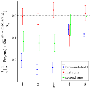
Although the bare returns were constructed using a Student’s t-distribution with 3 degrees of freedom, which by definition is not skewed, we see in Fig. 8 that the bare prices do not have zero skewness. This illustrates the role of the noise, which gives way to different values of skewness for bare prices depending on the number of periods of the session. We observe in Fig. 8 that the realized skewness of trade impacted returns is typically larger (i.e. less negative) than bare returns, but without any significant time dependence. This suggests that buying orders tend to be more synchronized than selling orders, specially in the first sessions, but that neither buying nor selling orders induce further buy/sell orders. In short, there is no destabilising feedback loop in the present setting, which explains why we never observed any large crash in our experiments.

In order to detect more precisely the synchronisation of our agents, we define an activity correlation matrix ${\bf A}$ as follows:

$$A_{ij}=\frac{1}{T}\sum_{t}\theta_{i}(t)\theta_{j}(t)-\frac{1}{T}\sum_{t}\theta_{i}(t)\times\frac{1}{T}\sum_{t}\theta_{j}(t),$$ (6)

where $\theta_{i}(t)$ is the activity of agent $i$ at time $t$, $\theta_{i}(t)=0$ if s/he is inactive, $\theta_{i}(t)=\pm 1$ if s/he buys or sells.

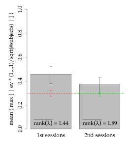
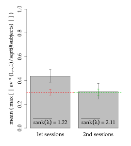
For each session, we diagonalize ${\bf A}$ and study the three largest eigenvalues, corresponding to the more important principal components of the subjects’ activity. In order to detect synchronisation, where a substantial fraction of agents tend to act in exactly the same way across the experiment, we compute the absolute value of the dot products of these three eigenvectors $\vec{v}_{1},\vec{v}_{2},\vec{v}_{3}$ and the uniform vector $\vec{e}=(1,1,\dots,1)/\sqrt{N}$. Then, we average the maximum of these three numbers over all runs. It may indeed happen that the “synchronized” mode does not correspond to the largest eigenvalue of ${\bf A}$, while still being amongst the three most important ones, and the above procedure allows one to capture these cases. The resulting values are represented in Fig.  9 for the first and second sessions, and compared with a null-hypothesis benchmark, obtained using 1000 random bootstrap replicates of the experiments.

Figure 9: Average maximum absolute value of the three dot products between the eigenvectors corresponding to the three largest eigenvalues, and the unit vector, with the corresponding statistical error bars. All orders are considered except for the first time step, in which we expect a natural bias towards synchronization. The dashed horizontal line around $0.3$ corresponds to the null hypothesis of completely uncorrelated actions.

The dashed lines depict the cases where agents would act completely at random, which would lead to a value of this average maximum overlap at approximately $0.35$. We see that the experimental results are clearly larger than the benchmark case: approximately $0.57$ for the first sessions and approximately $0.5$ for the second sessions (compared to a maximum value of $1$ for a fully collective activity mode).

The method above allows us to make a quantitative analysis and statement about overall synchronization in our experiment, be it through selling or buying orders, and we find that there is indeed significant synchronisation.

We also consider the separate cases of synchronization for selling orders and for buying orders. In order to do this, we construct an activity correlation matrix as in Eq. (6) but change the definition of $\theta_{i}(t)$ accordingly. This way, when we study the synchronization concerning only buying orders, we define $\theta_{i}(t)=0$ if agent $i$ is inactive or sells and $\theta_{i}(t)=1$ if he buys. Likewise, in the case where we look into synchronization over selling orders only, we set $\theta_{i}(t)=0$ if agent $i$ is inactive or buys and $\theta_{i}(t)=-1$ if he sells.

We see in Fig. 17a and in Fig. 17b in Appendix A that splitting the data set as explained does yield similar results: the experimental results are larger than the benchmark for each case, with the difference more marked in first sessions than in second sessions. Again, the synchronisation of buy orders appears to be, according to this metric, slightly stronger than that of sell orders.

We therefore conclude that although our subjects cannot directly communicate with one another, there is a significant synchronisation of their activity, in particular during the first sessions and, as the skewness of the distribution reveals, for the buying activity. The mechanism for this synchronisation can only come from the common source of information that the subjects all observe, namely the price time series itself – see below for more about this.

Furthermore, we observe an asymmetry if we repeat the above method conditional on the sign of previous returns, in the sense that synchronisation is stronger for buying orders conditional on negative previous returns and for selling orders conditional on positive previous returns. This indicates some sort of “mean reversion”, which is in line with the findings on subjects’ trading behaviour discussed in Subsection 4.3 below.

4.1.3 Clustering

Fig. 5 shows us, once again, that the average final wealth in first sessions is much smaller than in second sessions, which is tied to the higher average trading activity of the subjects when they play the game for the first time. In second sessions, we observe a number of subjects who kept trading activity very low, increasing their chances of a positive payout at the end of the experiment. As we discussed in Sec. 4.1.1, this is an indication that the subjects learn. In any case, there are always traders who keep trading at very high rates and lose money in the process.

However, Fig. 5 does not provide insight about common patterns in the behaviour of the subjects. We know from Fig. 4 that at least in second market sessions a number of subjects use the buy-and-hold strategy or similar, which corresponds to the green horizontal “corridors” in the figure. Therefore, we apply clustering techniques to search for groups of subjects with similar trading profiles in the data sets. Afterwards, we look into the trading activity and trading performance in each cluster.

As in Tumminello et al., (2011) and Tumminello et al., (2012), we applied false discovery rate (FDR) methods to validate links between subjects to the data set with composite data from first sessions and to the data set with composite data from second sessions. The variable used to establish links (i.e. similarity) between subjects was their position – in or out of the market – over time for each subject. The FDR rejection threshold was $1\%$.

The clusters are visualised in Fig. 10, which also displays the number of subjects in each cluster for first sessions and second sessions.

(a) First sessions

(b) Second sessions

Figure 10: Clusters for first and second sessions using the FDR algorithm with a threshold of $1\%$ applied to positions – in or out of the market – over time. The number of subjects in each cluster is displayed in the legends.

(a) First sessions

(b) Second sessions

Figure 11: Average trading activity and final wealth for each cluster represented in Fig. 10.

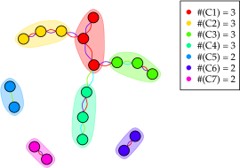
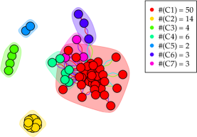
The clusters identified in the second sessions are much larger than those identified in first sessions, which is expected because the number of “intermittent” players in the game was lower in second sessions.

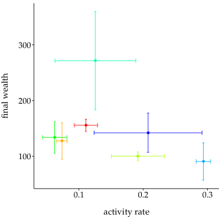
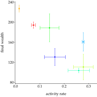
We see in Fig. 11 that clusters with a lower average trading activity tend to have a higher average final wealth. A notable example is the cluster number $2$ in Fig. 11b, which includes $14$ subjects (see Fig. 10b) who kept trading to a minimum in second runs and maximized their returns. Conversely, the cluster number $6$ in Fig. 11a consists of $2$ traders (see Fig. 10a) with very high average trading activity and, as a consequence, low final wealth.

4.2 Risk attitude and activity rate

To measure risk aversion of subjects we use the paired lottery choice instrument of Holt and Laury, (2002). The Holt-Laury paired-lottery choice task is a commonly-used individual decision-making experiment for measuring individual risk attitudes. This second experimental task was not announced in advance; subjects were instructed that, if they were willing, they could participate in a second experiment that would last an additional 10-15 minutes for which they could earn an additional monetary payment. All subjects agreed to participate in this second experiment. In this task subjects choose between a lottery with high variance of payoffs (Option B) and lottery with less variance (Option A). As in Holt and Laury, (2002) we use the relative frequency of B-choices (“risky” choices) as a measure for a preference for risk. Moreover, in order to make the amounts at stake comparable to what subjects could earn over an average session of trading periods and to assess whether or not the risk attitudes of subjects depended on the wealth levels involved, we elicited subjects’ choices for two lotteries, corresponding to two times ($2\times$) and ten times ($10\times$) the amounts offered by Holt and Laury, (2002) in their baseline treatment. Subjects were ex-ante informed that they would throw a dice to determine which of the two lotteries would determine their payoff from this additional experimental task.

Appendix C includes the instructions for the Holt-Laury paired-lottery choice experiment.

In Fig. 12 we show the distribution of subjects according to their risk aversion, both for the $2\times$ and the $10\times$ lottery.

Figure 12: Risk aversion cumulative distribution function. The x-axis shows the number of A-choices (“safe choices”) in the paired lotteries. The higher this level, the more risk-averse is the agent. The blue vertical line shows where a risk neutral subject would be.

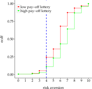
The blue vertical line shows where a risk neutral subject would be, based on the expected pay-off differences alone. The fact that the majority of the subjects – $76\%$ for the low-pay-off and $89\%$ for the high pay-off lotteries – have a number of “safe” A-choices larger than $4$ indicates that, overall, the participants in our experiment were risk-averse. Moreover, if we compare the two curves, red and green, we see that the subjects tend to safer choices when the lottery pay-off is higher, which indicates that the risk aversion of our population not only depends but increases with the pay-off level. This is corroborated by the Welch two-sample t-test, which states that the mean risk aversion values for low pay-off and high pay-off are statistically different with a p-value of $1.5\,10^{-6}$. We also estimate the parameters of the power-expo utility function in Eq. (5) using the lottery choices of our pool of subjects. As in Holt and Laury, (2002), we find evidence for increasing relative risk aversion and decreasing absolute risk aversion, i.e. positive estimates for both parameters $\alpha$ and $r$. Details on the estimation procedure and results are reported in Appendix B.

We now relate individual risk attitude, as elicited by the binary lottery choices, to trading behaviour. Previous experimental studies on the relation between elicited risk attitudes and aggregate market behaviour (Robin et al.,, 2012; Fellner and Maciejovsky,, 2007) show that the higher the degree of risk aversion the lower the observed market activity. On the other hand, Michailova, (2010) finds no significant effect of the number of safe choices in paired binary lotteries on the frequency of trading.

Fig. 13 displays average activity rates and levels of final wealth for different risk attitudes in both first and second runs.

(a)

(b)

Figure 13: Risk attitudes, trading activity and final wealth. Plot (a) displays average activity rate and final wealth for each level of risk aversion. Plot (b) shows linear regressions with $95\%$ intervals of confidence of the average activity rate and final wealth on risk aversion. Clearly, more risk averse subjects trade less and end up with a higher final wealth.

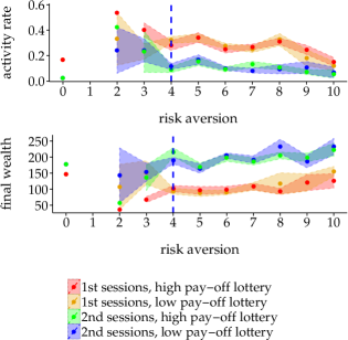
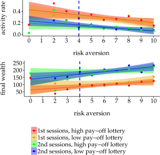
Our results clearly show that the activity rate decreases and the final wealth increases with the level of risk aversion, both in first runs (red and orange) and in second runs (green and blue). In other words, preference for risk is an important determinant of excess trading in our experiment. Our findings are in line with the empirical evidence suggesting that risk-loving, overconfident individuals are more willing to invest in stocks (Keller and Siegrist,, 2006) and engage in speculative activity (Odean and Barber,, 2011; Camacho-Cuena et al.,, 2012).

4.3 Price forecasts and trading behaviour

The fact that the subjects input their price predictions throughout the experiment allows us to have a glimpse of their frame of mind. In fact, trades only tell about the consequence of the state of mind (i.e. the price expectation) of traders when they are active. But traders (both in real life and in experiments) are in fact inactive most of the time. As a consequence, trades alone are unlikely to be able to explain why traders are inactive. Since we have both trades and subjects’ price expectations, we are able to give a consistent picture of activity and inactivity as a consequence of price return expectations.

In both market sessions, the subjects did not input anything in about $7\%$ of the time, as price prediction was not a mandatory activity (although monetarily incentivised); in the following, we restrict our analysis to the subjects that did report their predictions.

The discussion focuses on the predicted log returns, i.e. from subject $i$’s price predictions $\widehat{p_{i}}(t+1)$, we compute the predicted log returns $\widehat{r_{i}}(t+1)=\log[\widehat{p_{i}}(t+1)/p(t)]$, for all subjects. The average prediction in the first market sessions is $-0.01$, and $+0.02$ in the second market sessions, i.e. exactly in line with the average return $m=2\%$ in absence of trading. The percentage of positive predicted returns is 54% in the first run, and 58% in the second run. Fig. 14 illustrates the full empirical cumulative distribution functions of expectations for both runs and for positive and negative return separately.

Figure 14: Reciprocal empirical cumulative distribution functions of negative (left) and positive (right) expected price returns during the first and second sessions (black and red lines, respectively). The baseline return distribution is plotted in dashed lines. The jump at $r=0$ indicates the respective fraction of positive and negative predictions.

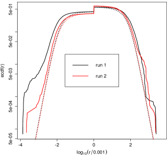
The starting point for each of the positive and negative distributions represents the fraction of positive and negative expectations, thus the higher jump at $r=0$ for the second session reflects the increase in the fraction of positive expected returns.

We then check how the distributions of positive and negative expected returns are related to the baseline return distribution, determined by the Student noise term $s\eta_{t}$ in the price updating rule. The baseline return distribution is plotted in dashed lines in Fig. 14; comparison between the latter and empirical distribution of expected returns gives a first clue about the type of extrapolation rules from past returns that the agents use. The asymptotic power-law tails of Student’s t-distributed variables, such as the noise $\eta_{t}$, are unchanged under summation, by virtue of the central limit theorem. This implies that linear expectations yield expectation distributions with power-laws tails that have the same exponent. On the other hand, panic or euphoria may lead to non-linear extrapolations and thus may modify either the tail exponent of these distributions, or even the nature of the tails.

The most obvious finding is that the actions of the agents increase the volatility of the baseline signal (in dashed lines) as the empirical distribution functions are above the baseline signal for both sequences. The amplification of the noise for positive expectations is almost the same in the two sequences, while for negative expectations there are marked differences between the two runs as the scale of negative expectations was much larger during the first run. We used robust power-law tail fitting (Clauset et al.,, 2009; Gillespie,, 2015) and determined the most likely starting point of a power-law $r_{min}$ and the exponent $\alpha$ (see Table 1). Quite remarkably, the parameters of the positive and negative tails are simply swapped between the two runs: thus not only the scale of negative expectations changes, but the nature of largest positive and negative expectations also changes. The fitted tail exponent is not far from $3$, the one of the Student noise showing once again the absence of destabilizing feedback loops.

	$r_{min}$	$\alpha$
run 1 $r<0$	0.21	3.5
run 2 $r>0$	0.10	2.7
run 1 $r<0$	0.13	2.6
run 2 $r>0$	0.18	3.5

Table 1: Fits of the power-law part of return expectations; $r_{min}$ denotes the most likely starting point of the power-law.

The fact that the subjects have heavy-tailed predictions suggests that they form their predictions by learning from past returns, which do contain heavy tails because of the Student’s t-distributed noise. We thus hypothesize some relationship between predicted returns and past returns. This is in line with the best established fact about real investors, which is the contrarian nature of their trades: their net investment over a given period is anti-correlated with past price returns (Jackson,, 2003; Kaniel et al.,, 2008; Grinblatt and Keloharju,, 2000; Challet and de Lachapelle,, 2013). In addition, previous experiments (Hommes et al.,, 2005) have demonstrated that four simple classes of linear predictors using past returns are usually enough to reproduce the observed price dynamics.

Based on the considerations outlined above, we first the return predictions of each subject with a linear model.

$$\widehat{r}(t+1)=\omega_{0}+\omega_{1}r(t),$$ (7)

where $\omega_{0}$ and $\omega_{1}\in\mathbb{R}$. Price return predictions are fitted separately for each trader, each session, and each possible action. We fit $\omega_{0}$ and $\omega_{1}$ simultaneously. Sec. 4.3.1 discusses results for $\omega_{0}$ while Sec. 4.3.2 is devoted to $\omega_{1}$.

4.3.1 Average predictions ($\omega_{0}$)

In order to give a picture of traders’ movements on the market we compute return expectations conditionally on the actions of the subjects. There are four possible actions: buying, selling, holding shares and holding cash. Fig. 15 reports the conditional distributions of price return predictions, for both sessions.

Figure 15: Densities of trader average return prediction $\omega_{0}$ during the first sessions (left plot) and second sessions (right plot) for the four types of decisions. Dashed vertical lines refer to the baseline return of $2\%$.

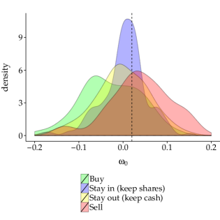
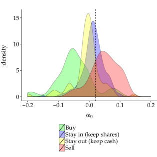
The results are qualitatively the same for both market sequences: the conditional distributions are clearly separated, as shown in Tab. 2 below; the main difference between the two runs is that the variance of expectations among the population is much reduced in the second run.

$\omega_{0}$, 1nd run	Sell	Hold cash	Hold shares
Buy	$1.5\,10^{-8}$	$3.9\,10^{-3}$	$1.2\,10^{-5}$
Sell		$3.8\,10^{-5}$	$8.2\,10^{-5}$
Hold cash			$1.5\,10^{-1}$

$\omega_{0}$, 2nd run	Sell	Hold cash	Hold shares
Buy	$2.1\,10^{-7}$	$1.5\,10^{-4}$	$1.0\,10^{-7}$
Sell		$6.1\,10^{-7}$	$5.9\,10^{-5}$
Hold cash			$6.6\,10^{-6}$

Table 2: Tests of the difference of distributions of $\omega_{0}$ among the subjects, conditional on two given actions. The table reports the p-values of Mann-Whitney tests for each possible pair of actions.

Let us break down the results for each possible action:

1. When the subjects hold assets, their expectations are in line with the baseline return of 2%.

2. When the subjects hold cash, their expectations are significantly lower (essentially zero).

3. When the subjects make a transaction, however, their expectations of the next returns are anti-correlated with their actions, i.e., they buy when they expect a negative price return and vice versa.

Thus, the actions of the subjects are fully consistent with their expectations: they do not invest when they do not perceive it as worthwhile and they keep their shares when they have a positive expectation of future gains. The actions of trading subjects are instead consistent with a “buy low, sell high” strategy. In fact, knowing that transactions will be executed at the price realized in the next period, subjects submit buy orders when they expect negative returns and sell orders when they expect positive returns.

4.3.2 Predictions and past price returns ($\omega_{1}$)

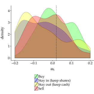
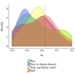
We find that the importance of the coefficient $\omega_{1}$, which encodes the linear extrapolation of the past return on future returns, is very weak. Figure 16 reports the conditional distributions of past returns’ impact coefficient for both runs, while Tab. 3 reports the p-values of the Mann-Whitney tests between coefficients $\omega_{1}$ between all state pairs for all subjects.

Figure 16: Densities of trader conditional return prediction $\omega_{1}$ during the first sessions (left plot) and second sessions (right plot) for the four types of decisions. Dashed vertical lines refer to the baseline return of $2\%$.

$\omega_{1}$, 1st run	Sell	Hold cash	Hold shares
Buy	$9.6\,10^{-2}$	$2.3\,10^{-5}$	$8.8\,10^{-10}$
Sell		$3.7\,10^{-2}$	$1.7\,10^{-4}$
Hold cash			$2.9\,10^{-2}$

$\omega_{1}$, 2nd run	Sell	Hold cash	Hold shares
Buy	$6.2\,10^{-1}$	$7.6\,10^{-1}$	$4.1\,10^{-2}$
Sell		$5.6\,10^{-1}$	$8.6\,10^{-2}$
Hold cash			$2.9\,10^{-4}$

Table 3: Tests of the difference of distributions of $\omega_{1}$ among the subjects, conditional on two given actions. The table reports the p-values of Mann-Whitney tests for each possible pair of actions.

The plot shows that during the first run, this coefficient was negative when the agents did not act and zero when they did trade. The second run is different: the coefficients do not seem to depend much on the state, the only clear difference is between holding cash and holding shares.

The lack of influence of this coefficient is confirmed when one measures the average predicted return conditional on the action of the subjects, which gives results very close to $\omega_{0}$.

5 Conclusion

We presented the results of a trading experiment in which the pricing function favours early investment in a risky asset and no posterior trading. In our experimental markets the subjects would make an almost certain gain of over $600\%$ if they all bought shares in the first period and held them until the end of the experiment.

However, market impact as defined in Eq. 4 acts de facto as a transaction cost which erodes the earnings of the traders. Our subjects are made well aware of this mechanism. Still, when they participate in the experiment for the first time, their trading activity is so high that their profits average to almost zero. They are however found to fare much better when they repeat the experiment as they earn $92\%$ on average – which is still much below the performance of the simple risk-neutral rational strategy outlined above. We therefore find that, echoing Odean (Odean,, 1999; Odean and Barber,, 2011), investors trade too much, even in an environment where trading is clearly detrimental and buy-and-hold is an almost certain winning strategy (at variance with real markets where there is nothing like a guaranteed average return of $2\%$ per period). Our result is potentially quite important when translated into the real world: unwarranted individual decisions can lead to a substantial loss of collective welfare, mediated by the mechanics of financial markets.

At the end of the experiment we collect data on traders’ risk attitude by means of paired lottery choices à la Holt and Laury, (2002). We observe that, overall, our subjects are risk-averse and their relative risk aversion increases with the pay-off level in a way that is quantitatively similar to the results reported in Holt and Laury, (2002). We then relate individual risk attitude with the results of the trading experiment and we observe that the activity rate increases and the final wealth decreases with subjects’ preference for risk.

Moreover, in each period we also ask subjects to predict the next price of the asset. This provides us with additional information about our controlled experimental market, i.e. we have access not only to the decisions of each trader but also to their expectations. It is important to emphasize that this information would not be available in broker data. In fact, knowing the expectation behind each decision of each trader – including the decisions to do nothing – is one of the advantages of laboratory experiments compared to empirical analysis of real data. Using this information, we confirm in Sec. 4.3 that the traders in our experiment have a contrarian nature, which, together with the pattern of excessive trading, is one of the known features of individual traders in real financial markets, as discussed in de Lachapelle and Challet, (2010) and Challet and de Lachapelle, (2013). In particular, it seems that our subjects actively engaged in trading in the attempt to “beat the market”, i.e. trying to make profits by buying the asset when they expected the price to be low and selling the asset when they expected the price to move upwards.

Contrary to what happens in real financial markets, we have not observed any “leverage effect” (i.e. an increase of volatility after down moves). Although there is a clear detrimental collective behaviour in all sessions of this experiment, we do not witness any big crash or avalanche of selling orders that would result from a panic mode. As we discuss in Sec. 4.1.2, the coordination amongst traders was actually slightly stronger when buying than when selling, resulting in a positive skewness of the returns. In order to induce crashes and study their dynamics, the duration of the experiment could be expanded while the time available for each decision could be reduced. The former would increase the probability of a sudden event by increasing the number of trials and the amounts at stake, while the latter could contribute to higher stress levels amongst subjects and increased sensitivity to price movements. However, we believe that a more efficient way to generate panic and herding behaviour would be to reduce the “normal” volatility level while and increasing the amplitude of “jumps” in the bare return time series. Within the current setting, large fluctuations do not seem surprising enough to trigger panic among our participants. Another idea, perhaps closer to what happens in financial markets, would be to increase the impact of sell orders and reduce the impact of buy orders when the price is high, mimicking the fact that buyers are rarer when the price is high (on this point, see the recent results of Donier and Bouchaud, 2015b on the Bitcoin). Other natural extensions of this experiment would include the possibility of fraction orders and hedging, as well as short selling. We leave these extensions and additional experimental designs to future research.

Appendix

Appendix A Additional figures

(a) Buying orders.

(b) Selling orders.

Figure 17: Average maximum absolute value of the sum of the components of the eigenvectors corresponding to the three largest eigenvalues. On the left we restrict ourselves to buying orders, while the result for selling orders is shown on the right. The first time step is excluded from the data set because we expect a natural bias towards synchronization. The dashed horizontal lines around $0.3$ corresponds to the null hypothesis of completely uncorrelated actions.

Figure 18: Screenshot

Appendix B Estimation of risk aversion parameters

As in Holt and Laury, (2002), we use the lottery choices of the subjects to calibrate the utility function described in Eq. (5). In short, we apply a maximum-likelihood method to find the parameters which maximize the probability that the observed lottery choices are dictated by Eq. (5).

In this spirit, the first step we take is to model the probability $P_{i}^{R}$ that a subject chooses the risky lottery out of the pair $i$ of lotteries. As in Holt and Laury, (2002), we define

$$P_{i}^{R}:=\frac{E[U_{i}^{R}]^{\frac{1}{\mu}}}{E[U_{i}^{R}]^{\frac{1}{\mu}}+E[U_{i}^{S}]^{\frac{1}{\mu}}},$$ (8)

where $E[U_{i}^{R}]=\sum_{k=1}^{2}{p_{k}U_{k}^{R}}$ is the expected utility of the risky lottery and $E[U_{i}^{S}]$ is the expected utility of the safe lottery in the pair $i$. Each lottery has two possible outcomes $k=1,2$, each with probability $p_{k}$ and utility $U_{k}$ given by Eq. (5), parameterized by two numbers $\alpha$ and $r$. The parameter $\mu$ is a real number which allows one to consider a range of scenarios between equiprobable choices ($\mu=+\infty$) and utility maximization ($\mu\rightarrow 0$). This corresponds to the so called “logit rule” (see Bouchaud, (2013) or Anderson et al., (1992) for further details).

Secondly, we define the likelihood function

$$\mathcal{L}(\beta,y)=\prod_{i}(P_{i}^{R})^{y}_{i}\cdot(1-P_{i}^{R})^{1-y_{i}},$$ (9)

where $y_{i}$ are the observed choices for each lottery pair, i.e. $y_{i}=0$ if the subject chose the safe lottery and $y_{i}=1$ if he chose the risky lottery from pair $i$. In addition, $\beta=[r,\alpha,\mu]$ includes all the model parameters in Eq. (8).

This way, we have the log-likelihood function

$$\mathrm{log}[\mathcal{L}(\beta,y)]=\sum_{i}y_{i}\mathrm{log}(P_{i}^{R})+(1-y_{i})\mathrm{log}(1-P_{i}^{R}).$$ (10)

Finally, the last step is to find the model parameters that maximize Eq. (10). We apply the Nelder-Mead algorithm (Nelder and Mead,, 1965) and use the bias-corrected and accelerated (BCa) bootstrap method (Efron,, 1987) for $95\%$ confidence intervals. The results are summarized in Tab. 4. Quite remarkably, the values of the a-dimensional parameters $r$ and $\mu$ are found to be very close to those reported in Holt and Laury, (2002) for their lottery experiments ($\mu=0.13$, $r=0.27$). In particular, our estimates imply increasing relative risk aversion and decreasing absolute risk aversion.

	estimate	confidence interval
$\alpha$	$0.106$	$[0.085,0.130]$
$r$	$0.345$	$[0.263,0.443]$
$\mu$	$0.114$	$[0.101,0.133]$

Table 4: Parameters of Eq. (8) obtained via maximum-likelihood estimation and correspondent $95\%$ confidence intervals. We applied the Nelder-Mead algorithm to maximize Eq. (10) and used the bias-corrected and accelerated (BCa) bootstrap method for the $95\%$ confidence intervals.

Appendix C Experimental instructions and paired lottery task (for online publication only)

See pages - of ./instructions/exp_istr_final_cash.pdf See pages - of ./instructions/quiz.pdf See pages - of ./instructions/lottery.pdf

References

- Anderson et al., (1992) Anderson, S. P., De Palma, A., and Thisse, J. F. (1992). Discrete choice theory of product differentiation. MIT press.
- Barber et al., (2009) Barber, B. M., Lee, Y.-T., Liu, Y.-J., and Odean, T. (2009). Just how much do individual investors lose by trading? Review of Financial Studies, 22(2):609–632.
- Barber and Odean, (2000) Barber, B. M. and Odean, T. (2000). Trading is hazardous to your wealth: The common stock investment performance of individual investors. Journal of Finance, pages 773–806.
- Barber and Odean, (2008) Barber, B. M. and Odean, T. (2008). All that glitters: The effect of attention and news on the buying behavior of individual and institutional investors. Review of Financial Studies, 21(2):785–818.
- Barber and Odean, (2013) Barber, B. M. and Odean, T. (2013). The behavior of individual investors. Handbook of the Economics of Finance, 2:1533–1570.
- Barberis and Thaler, (2003) Barberis, N. and Thaler, R. (2003). A survey of behavioral finance. Handbook of the Economics of Finance, 1:1053–1128.
- Bondt and Thaler, (1985) Bondt, W. F. and Thaler, R. (1985). Does the stock market overreact? The Journal of finance, 40(3):793–805.
- Bouchaud, (2010) Bouchaud, J.-P. (2010). Price impact. Encyclopedia of quantitative finance.
- Bouchaud, (2013) Bouchaud, J.-P. (2013). Crises and collective socio-economic phenomena: simple models and challenges. Journal of Statistical Physics, 151(3-4):567–606.
- Bouchaud et al., (2008) Bouchaud, J.-P., Farmer, J. D., and Lillo, F. (2008). How markets slowly digest changes in supply and demand. Fabrizio, How Markets Slowly Digest Changes in Supply and Demand (September 11, 2008).
- Bouchaud et al., (2009) Bouchaud, J.-P., Farmer, J. D., and Lillo, F. (2009). How markets slowly digest changes in supply and demand. pages 57 – 160.
- Bouchaud et al., (2001) Bouchaud, J.-P., Matacz, A., and Potters, M. (2001). Leverage effect in financial markets: The retarded volatility model. Physical Review Letters, 87(22):228701.
- Bouchaud and Potters, (2003) Bouchaud, J.-P. and Potters, M. (2003). Theory of financial risk and derivative pricing: from statistical physics to risk management. Cambridge university press.
- Breaban and Noussair, (2014) Breaban, A. and Noussair, C. (2014). Fundamental Value Trajectories and Trader Characteristics in an Asset Market Experiment. Discussion paper, Tilburg University, Center for Economic Research.
- Caccioli et al., (2014) Caccioli, F., Shrestha, M., Moore, C., and Farmer, J. D. (2014). Stability analysis of financial contagion due to overlapping portfolios. Journal of Banking & Finance, 46:233–245.
- Camacho-Cuena et al., (2012) Camacho-Cuena, E., Requate, T., and Waichman, I. (2012). Investment Incentives Under Emission Trading: An Experimental Study. Environmental & Resource Economics, 53(2):229–249.
- Challet and de Lachapelle, (2013) Challet, D. and de Lachapelle, D. M. (2013). A robust measure of investor contrarian behaviour. In Econophysics of Systemic Risk and Network Dynamics, pages 105–118. Springer.
- Cipriani and Guarino, (2014) Cipriani, M. and Guarino, A. (2014). Estimating a Structural Model of Herd Behavior in Financial Markets. American Economic Review, 104(1):224–51.
- Clauset et al., (2009) Clauset, A., Shalizi, C. R., and Newman, M. E. (2009). Power-law distributions in empirical data. SIAM review, 51(4):661–703.
- Cont and Wagalath, (2014) Cont, R. and Wagalath, L. (2014). Fire sales forensics: measuring endogenous risk. Mathematical Finance.
- Crockett and Duffy, (2013) Crockett, S. and Duffy, J. (2013). A Dynamic General Equilibrium Approach to Asset Pricing Experiments. Working Paper.
- de Lachapelle and Challet, (2010) de Lachapelle, D. M. and Challet, D. (2010). Turnover, account value and diversification of real traders: evidence of collective portfolio optimizing behavior. New Journal of Physics, 12(7):075039.
- (23) Donier, J. and Bouchaud, J.-P. (2015a). From walras’ auctioneer to continuous time double auctions: A general dynamic theory of supply and demand. arXiv preprint arXiv:1506.03758.
- (24) Donier, J. and Bouchaud, J.-P. (2015b). Why do markets crash? bitcoin data offers unprecedented insights.
- Dufwenberg et al., (2005) Dufwenberg, M., Lindqvist, T., and Moore, E. (2005). Bubbles and experience: An experiment. American Economic Review, pages 1731–1737.
- Efron, (1987) Efron, B. (1987). Better bootstrap confidence intervals. Journal of the American statistical Association, 82(397):171–185.
- Fellner and Maciejovsky, (2007) Fellner, G. and Maciejovsky, B. (2007). Risk attitude and market behavior: Evidence from experimental asset markets. Journal of Economic Psychology, 28(3):338–350.
- Gillespie, (2015) Gillespie, C. S. (2015). Fitting heavy tailed distributions: The poweRlaw package. Journal of Statistical Software, 64(2):1–16.
- Giusti et al., (2012) Giusti, G., Jiang, J. H., and Xu, Y. (2012). Eliminating laboratory asset bubbles by paying interest on cash. Working paper GATE 2012-35.
- Gopikrishnan et al., (1998) Gopikrishnan, P., Meyer, M., Amaral, L. N., and Stanley, H. E. (1998). Inverse cubic law for the distribution of stock price variations. The European Physical Journal B-Condensed Matter and Complex Systems, 3(2):139–140.
- Greenwood and Shleifer, (2014) Greenwood, R. and Shleifer, A. (2014). Expectations of returns and expected returns. Review of Financial Studies, page hht082.
- Grinblatt and Keloharju, (2000) Grinblatt, M. and Keloharju, M. (2000). The investment behavior and performance of various investor types: a study of finland’s unique data set. Journal of Financial Economics, 55(1):43–67.
- Grinblatt and Keloharju, (2001) Grinblatt, M. and Keloharju, M. (2001). What Makes Investors Trade? Journal of Finance, 56(2):589–616.
- Harrison et al., (2007) Harrison, G. W., List, J. A., and Towe, C. (2007). Naturally occurring preferences and exogenous laboratory experiments: A case study of risk aversion. Econometrica, 75(2):433–458.
- Harrison and Rutström, (2008) Harrison, G. W. and Rutström, E. E. (2008). Risk aversion in the laboratory. Research in experimental economics, 12:41–196.
- Haruvy et al., (2007) Haruvy, E., Lahav, Y., and Noussair, C. N. (2007). Traders’ expectations in asset markets: experimental evidence. The American Economic Review, 97(5):1901–1920.
- Holt and Laury, (2002) Holt, C. A. and Laury, S. K. (2002). Risk aversion and incentive effects. American economic review, 92(5):1644–1655.
- Hommes, (2013) Hommes, C. (2013). Reflexivity, expectations feedback and almost self-fulfilling equilibria: economic theory, empirical evidence and laboratory experiments. Journal of Economic Methodology, 20(4):406–419.
- Hommes et al., (2005) Hommes, C., Sonnemans, J., Tuinstra, J., and Van de Velden, H. (2005). Coordination of expectations in asset pricing experiments. Review of Financial Studies, 18(3):955–980.
- Hommes et al., (2008) Hommes, C., Sonnemans, J., Tuinstra, J., and van de Velden, H. (2008). Expectations and bubbles in asset pricing experiments. Journal of Economic Behavior & Organization, 67(1):116–133.
- Hussam et al., (2008) Hussam, R. N., Porter, D., and Smith, V. L. (2008). Thar she blows: Can bubbles be rekindled with experienced subjects? American Economic Review, 98(3):924–37.
- Jackson, (2003) Jackson, A. (2003). The aggregate behaviour of individual investors. Available at SSRN 536942.
- Jondeau and Rockinger, (2003) Jondeau, E. and Rockinger, M. (2003). Testing for differences in the tails of stock-market returns. Journal of Empirical Finance, 10(5):559–581.
- Kaniel et al., (2008) Kaniel, R., Saar, G., and Titman, S. (2008). Individual investor trading and stock returns. The Journal of Finance, 63(1):273–310.
- Keller and Siegrist, (2006) Keller, C. and Siegrist, M. (2006). Investing in stocks: The influence of financial risk attitude and values-related money and stock market attitudes. Journal of Economic Psychology, 27(2):285–303.
- King, (1991) King, R. R. (1991). Private Information Acquisition In Experimental Markets Prone To Bubble And Crash. Journal of Financial Research, 14(3):197–206.
- Lei et al., (2001) Lei, V., Noussair, C. N., and Plott, C. R. (2001). Nonspeculative bubbles in experimental asset markets: Lack of common knowledge of rationality vs. actual irrationality. Econometrica, pages 831–859.
- Lei and Vesely, (2009) Lei, V. and Vesely, F. (2009). Market efficiency: Evidence from a no-bubble asset market experiment. Pacific Economic Review, 14(2):246–258.
- Lillo and Farmer, (2004) Lillo, F. and Farmer, J. D. (2004). The long memory of the efficient market. Studies in nonlinear dynamics & econometrics, 8(3).
- Lillo et al., (2003) Lillo, F., Farmer, J. D., and Mantegna, R. N. (2003). Econophysics: Master curve for price-impact function. Nature, 421(6919):129–130.
- Michailova, (2010) Michailova, J. (2010). Overconfidence, risk aversion and (economic) behavior of individual traders in experimental asset markets. MPRA Paper 26390, University Library of Munich, Germany.
- Nelder and Mead, (1965) Nelder, J. A. and Mead, R. (1965). A simplex method for function minimization. The computer journal, 7(4):308–313.
- Noussair and Powell, (2010) Noussair, C. N. and Powell, O. (2010). Peaks and valleys: Price discovery in experimental asset markets with non-monotonic fundamentals. Journal of Economic Studies, 37(2):152–180.
- Odean, (1999) Odean, T. (1999). Do investors trade too much? The American Economic Review, 89(5):1279–1298.
- Odean and Barber, (2011) Odean, T. and Barber, B. (2011). Boys will be boys: Gender, overconfidence, and common stock investment. Quarterly Journal of Economics, 116(1):261–292.
- Oechssler, (2010) Oechssler, J. (2010). Searching beyond the lamppost: Let’s focus on economically relevant questions. Journal of economic behavior & organization, 73(1):65–67.
- Palan, (2013) Palan, S. (2013). A review of bubbles and crashes in experimental asset markets. Journal of Economic Surveys, 27(3):570–588.
- Reigneron et al., (2011) Reigneron, P.-A., Allez, R., and Bouchaud, J.-P. (2011). Principal regression analysis and the index leverage effect. Physica A: Statistical Mechanics and its Applications, 390(17):3026–3035.
- Robin et al., (2012) Robin, S., Straznicka, K., and Villeval, M. C. (2012). Bubbles and Incentives : An Experiment on Asset Markets. MPRA Paper no. 37321.
- Roth and Murnighan, (1978) Roth, A. and Murnighan, J. K. (1978). Equilibrium Behavior and Repeated Play of the Prisoners Dilemma. Journal of Mathematical Psychology, 17:189–198.
- Smith, (2010) Smith, V. (2010). Theory and experiment: What are the questions? Journal of Economic Behavior & Organization, 73(1):3 – 15.
- Smith et al., (1988) Smith, V. L., Suchanek, G. L., and Williams, A. W. (1988). Bubbles, crashes, and endogenous expectations in experimental spot asset markets. Econometrica: Journal of the Econometric Society, pages 1119–1151.
- Solnik and Zuo, (2012) Solnik, B. and Zuo, L. (2012). A global equilibrium asset pricing model with home preference. Management Science, 58(2):273–292.
- Stöckl et al., (2015) Stöckl, T., Huber, J., and Kirchler, M. (2015). Multi-period experimental asset markets with distinct fundamental value regimes. Experimental Economics, 18(2):314–334.
- Tumminello et al., (2012) Tumminello, M., Lillo, F., Piilo, J., and Mantegna, R. N. (2012). Identification of clusters of investors from their real trading activity in a financial market. New Journal of Physics, 14(1):013041.
- Tumminello et al., (2011) Tumminello, M., Miccichè, S., Lillo, F., Piilo, J., and Mantegna, R. N. (2011). Statistically validated networks in bipartite complex systems. PloS one, 6(3):e17994.
- Van Boening et al., (1993) Van Boening, M. V., Williams, A. W., and LaMaster, S. (1993). Price bubbles and crashes in experimental call markets. Economics Letters, 41(2):179–185.
- Xie and Zhang, (2012) Xie, H. and Zhang, J. (2012). Bubbles and experience: an experiment with a steady inflow of new traders. Cirano scientific series, CIRANO, Montreal.