Abstract: Many damped mechanical systems oscillate with increasing frequency as the amplitude decreases. One popular example is Euler’s Disk, where the point of contact rotates with increasing rapidity as the energy is dissipated. We study a simple mechanical pendulum that exhibits this behaviour.

Galileo noticed the regular swinging of a candelabra in the cathedral in Pisa and speculated that the swing period was constant. This led him to use a pendulum to measure intervals of time for his experiments in dynamics [TOB03, pg 97]. Galileo’s conclusion was close to correct: for small swing angles, the period of a pendulum varies little with amplitude. Even with a swing through $180^{\circ}$, the period is only $18\%$ greater than that for a small swing angle.

V-shaped Potential

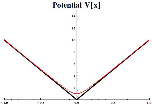
Figure 1: V-shaped potential function $V(x)=\kappa|x|$ (solid black line) and a regular approximation $V_{\epsilon}(x)=\kappa\sqrt{x^{2}+\epsilon^{2}}$ (dashed red line).

Unlike the simple pendulum, many mechanical systems rock back and forth with decreasing period as the motion dies down, oscillating with ever-increasing frequency. To exemplify this behaviour, let us look at a particle moving in a V-shaped potential well. To be specific, let us take the potential energy to be

$$V(x)=\kappa|x|\,.$$

which is shown in Fig. 1. Also shown is the function $V_{\epsilon}(x)=\kappa\sqrt{x^{2}+\epsilon^{2}}$ which is regular and which approximates $V(x)$ as $\epsilon\rightarrow 0$.

For the V-potential well, the restoring force is

$$F(x)=-\frac{\partial V}{\partial x}=-\kappa\operatorname{sgn}x=\begin{cases}-\kappa&\mbox{if }x>0\\ +\kappa&\mbox{if }x<0\end{cases}$$

The equation of motion for a particle of unit mass is $\ddot{x}=F(x)$ [SandG59]. Since the force is constant as long as the sign of $x$ remains unchanged, we can write the solution for initial conditions $x(0)=x_{0}>0,\dot{x}(0)=v_{0}$ by solving $\ddot{x}=-\kappa$:

$$x(t)=x_{0}+v_{0}t-\textstyle{\frac{1}{2}}\kappa t^{2}\,.$$

Thus, $x$ is a parabolic function of time. This remains valid until $t=t_{0}=[v_{0}+\sqrt{v_{0}^{2}+2\kappa x_{0}}]/\kappa$. We will assume that $v_{0}=0$. Then $x$ reaches zero at time $t_{0}=\sqrt{2x_{0}/\kappa}$.

The solution is continued beyond $t_{0}$ by solving $\ddot{x}=+\kappa$. This gives another parabolic segment, inverted with respect to the first one and joined smoothly to it. Note that $x$ and $\dot{x}$ are continuous at $t_{0}$ but the acceleration $\ddot{x}$ is discontinuous there.

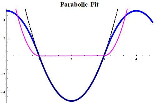
Figure 2: Numerical solution with $x_{0}=5$ and $\kappa=10$ (heavy blue line), and parabola fitting a segment (dashed black line). Difference between the solution and the parabola (thin magenta line).

The solution comprises a sequence of parabolic arcs smoothly joined at times $\{t_{0},3t_{0},5t_{0},\dots\}$. Fig. 2 shows the numerical solution (heavy blue curve) and a parabola fitted to the segment $(t_{0},3t_{0})$. The thin magenta curve shows the difference. One can see that the fit is excellent.

The motion is periodic, with period $\tau=4t_{0}$ and frequency $\omega=2\pi/\tau$, so

$$\tau=4\sqrt{\frac{2x_{0}}{\kappa}}\qquad\mbox{and}\qquad\omega=\frac{\pi}{4}\sqrt{\frac{2\kappa}{x_{0}}}\,.$$ (1)

We see immediately that $\omega\rightarrow\infty$ as $x_{0}\rightarrow 0$.

The Ping Pong Pendulum

We consider a pendulum with two pivots (Fig. 3). The motion is confined to a plane and the pendulum pivots alternately about each pivot. The pendulum bob moves on a circular arc centered at the left pivot when it is swinging to the right (Fig. 4). When swinging to the left, it rotates about the right pivot, following another circular arc. Thus, the motion of the bob is along two circular arcs, intersecting at the point of equilibrium.

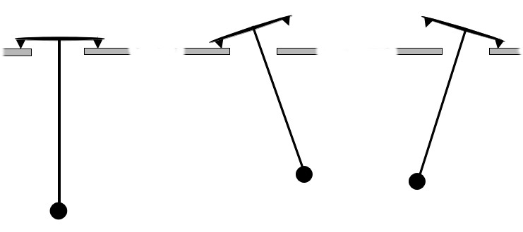
Figure 3: The ping pong pendulum. Left panel: at equilibrium. Centre panel: swinging to the right. Right panel: swinging to the left.

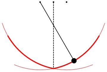
Figure 4: Bob moves on a circular arc centered at the left pivot when swinging to the right, and on an arc centered at the right pivot when swinging to the left.

The origin of coordinates is taken to be at the point mid-way between the two pivot points. The distance between the pivots is $2\delta$, the distance from pivot to bob is $\ell$ and the point of equilibrium is at $(0,-h)$ (see Fig. 5). The configuration of the system is determined by $\theta$, the angle between the vertical through the origin and the line from origin to bob. Elementary algebraic geometry shows that, for $\theta>0$, the coordinates of the bob are

$$x = \phantom{-}\sqrt{\ell^{2}-\delta^{2}\cos^{2}\theta}\cdot\sin\theta-\delta\sin^{2}\theta$$ (2)

$$y = -\sqrt{\ell^{2}-\delta^{2}\cos^{2}\theta}\cdot\cos\theta+\delta\sin\theta\cos\theta$$ (3)

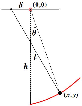
Figure 5: Notation used to describe the system. The configuration is determined by the angle $\theta$. The case $\theta>0$ is shown here.

Damping and Frequency Growth

For small swing amplitudes, we may approximate the two circular arcs by line segments, so that (2)–(3) become

$$x=h\theta\,,\qquad y=-h+\delta\theta\,.$$

The tangents to the circular arcs at the point $(0,-h)$ are the lines $y=-h+(\delta/h)x$ and $y=-h-(\delta/h)x$.

The potential energy becomes a V-shaped potential well, $V(\theta)=\kappa|\theta|$, where $\kappa=\delta/h$. We have seen that the motion in such a potential well is described by a sequence of parabolic arcs and the period is $\tau=4\sqrt{{2x_{0}}/{\kappa}}=4\sqrt{{2h\theta_{0}}/{\kappa}}$.

Now we add damping to the system, and model the motion by the equation

$$\ddot{\theta}+k\dot{\theta}+\kappa\operatorname{sgn}\theta=0$$ (4)

This equation can be solved piecewise in analytical terms. For $\theta>0$ the solution is

$$\theta=\theta_{0}+\left(\frac{\dot{\theta}_{0}}{k}+\frac{\kappa}{k^{2}}\right)(1-e^{-kt})-\frac{\kappa t}{k}\,.$$

However, it is inconvenient to have separate solutions for separate segments, so we solve the equation numerically, replacing $V(x)$ by $V_{\epsilon}(x)$ with a small value of $\epsilon$. The result shown in Fig. 6. It is clear that the frequency increases strongly as the amplitude decreases. To make this even clearer, we also show the solution scaled by a growing exponential function.

This pattern of frequency increasing as energy decreases is similar to the behaviour of a range of physical systems [BandB05]. We have mentioned the Euler Disk, but there are many others.

.

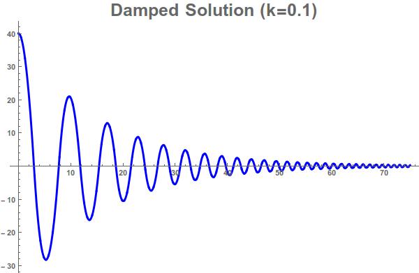
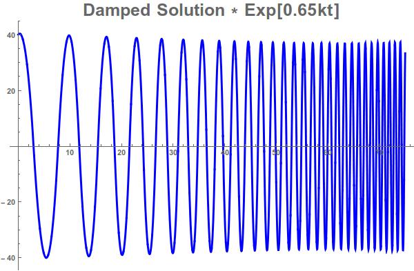
Figure 6: Top: Solution of equation (4) with damping coefficient $k=0.1$. Bottom: Solution of equation (4) scaled up by an exponential factor.

References

- [BandB05] Baker, G. L. and J. A. Blackburn, 2005: The Pendulum: A Case Study in Physics. Oxford Univ. Press, 288pp. ISBN: 9-780-198-56754-7.
- [SandG59] Synge, J. L. and B. A. Griffith, 1959: Principles of Mechanics. McGraw-Hill, Third Edition, 552pp.
- [TOB03] Tobin, William, 2003: The Life and Science of Léon Foucault. Camb. Univ. Press, 338pp. ISBN: 9-780-521-80855-2.