Rotational relaxation time as unifying time scale for polymer and fiber drag reduction

Abstract

Using hybrid Direct Numerical Simulation with Langevin dynamics, a comparison is performed between polymer and fiber stress tensors in turbulent flow. The stress tensors are found to be similar, suggesting a common drag reducing mechanism in the onset regime for both flexible polymers and rigid fibers. Since fibers do not have an elastic backbone, this must be a viscous effect. Analysis of the viscosity tensor reveals that all terms are negligible, except the off-diagonal shear viscosity associated with rotation. Based on this analysis, we identify the rotational orientation time as the unifying time scale setting a new time criterion for drag reduction by both flexible polymers and rigid fibers.

I Introduction

When a Newtonian fluid transitions from laminar flow to turbulent flow, changes in pressure and velocity fields become chaotic, and eddies, coherent patterns of flow velocity and pressure, start to form. As eddies break up into smaller eddies, an energy cascade forms, which transports the kinetic energy of the flow to smaller, and smaller time and length scales. Eventually, at the smallest scales, also called the Kolmogorov scales, this kinetic energy gets dissipated into heat, due to viscosity. Once a flow is turbulent, the energy cascade is sustained through the turbulence regeneration cycle Jiménez and Pinelli (1999). Drag reduction is the phenomenon where, by either modifying the boundary conditions on the wall (Choi et al., 1993, 1994) or by adding additives (Toms, 1949; Pirih and Swanson, 1972; Lee et al., 1974; Radin et al., 1975) to the flow, the turbulence regeneration cycle is disrupted and the dissipation of turbulent kinetic energy is reduced. Because of their effectiveness as drag reducing agents, polymers are a popular type of additive (Toms, 1949). By adding only a couple of parts per million of certain polymers to a fluid, well below their overlap concentration where polymer-polymer interactions are negligible, a drag reduction of up to 80 percent can be observed (Gampert and Wagner, 1982). Fibers are another additive that also generate drag reduction (Radin et al., 1975), and one of the open questions in drag reduction is whether fibers and polymers share the same drag reduction mechanism. Considering that fibers are simply very stiff polymers, one could regard fiber drag reduction as a limiting case of polymer drag reduction and make the assumption that they share the same drag reducing mechanism. On the other hand, it has been reported that polymers have an onset criterion (Virk et al., 1967), while fibers do not (Paschkewitz et al., 2004). Additionally, it has been found that fibers are not as effective drag reducing agents as polymers (Paschkewitz et al., 2004), and there is the viscosity (Lumley, 1969) versus elasticity (De Gennes, 1986) debate.

Because polymers are typically a lot smaller than the Kolmogorov length scale, while their relaxation times overlap with the Kolmogorov time scale, the onset of drag reduction for polymers is determined by a time criterion (Lumley, 1969). Fibers are not elastic and thus do not have an onset criterion like flexible polymers do. However, their molecular weight does have an effect on their drag reducing effect Sasaki (1992), and a critical aspect ratio for fibers has been found Radin et al. (1975). Since fibers are also typically smaller than the Kolmogorov scale, rather than a length scale, it can be expected that, like polymers, there is a fiber time scale associated with their effectiveness as drag reducing agents.

The viscosity versus elasticity debate is centered around the question as to whether polymer drag reduction is a local phenomenon caused by extensional viscosity, or a non-local phenomenon caused by the transport of turbulent kinetic energy into the polymer chain. In an extensional flow, when a critical shear rate is reached, polymer coils stretch significantly compared to their equilibrium state, which results in a significant increase of the elongational viscosity (Metzner and Metzner, 1970). Replacing the inverse critical shear rate with the Kolmogorov time scale, this viscosity increase was proposed by Lumley (1969) as a mechanism for drag reduction. The first to suggest that elasticity is essential for drag reduction was De Gennes (1986). Based on work by Daoudi and Brochard (1978) he concluded that the elongational viscosity theory could not be correct due to the absence of the coil-stretch transition for polymers undergoing randomly fluctuating stresses in a turbulent velocity field, and reasoned that drag reduction had to be the result of the elastic properties of polymers instead (Tabor and De Gennes, 1986; Sreenivasan and White, 2000). Based on experimental work, theory, and simulations, there is support for both theories (Moosaie and Manhart, 2013). Since fibers do not have an elastic backbone their drag reducing effect is caused by viscosity effects, and if elastic theory is right, it has to be concluded that fibers and polymers have different drag reducing mechanisms. However, if the drag reducing mechanism for polymers and fibers is the same, the conclusion has to be that for polymers the drag reducing effect is also caused by viscosity.

The present work investigates the effect of elasticity on drag reduction by studying the stress tensor, effective viscosity, and torque generated by different polymers and fibers in turbulent pipe flow. To model the polymers and fibers, a hybrid Direct Numerical Simulation/Langevin Dynamics approach is taken. This way no closure models are needed to calculate the stress tensor for either the polymers (Sureshkumar et al., 1997; Zhou and Akhavan, 2003) or the fibers (Paschkewitz et al., 2004; Gillissen et al., 2007a), and a direct comparison of the polymer and fiber stress tensors is possible. While the polymers or fibers and solvent are two way coupled, the number of molecules in the system is too small to observe drag reduction in the velocity profile of the flow (Moosaie and Manhart, 2013). This means that the results presented here are only applicable to the onset of drag reduction and not the Maximum Drag Reduction (MDR) regime, the maximum amount of drag reduction that can be observed in turbulent flow (Virk, 1975a).

The MDR regime has been previously addressed by L’vov et al. (2004) and Benzi et al. (2005). They have used the Doi and Edwards (1986) stress tensor to model the fibers and the Giesekus (1962) stress tensor, assuming that the flexible polymers are in the Hookean regime (Bird et al., 1987), for the elastic flexible polymers. They have reported that the physical origins of the stresses of flexible polymers and rigid fibers are different, and have proposed different scaling laws for the Reynolds stresses at the wall for elastic polymers and inelastic fibers. Nevertheless, in the regime of the maximum drag reduction (MDR) asymptote, they argued that both flexible polymers and rigid fibers give rise to an effective viscosity and that this viscous effect is responsible for drag reduction in the MDR regime for both flexible polymers and fibers.

In the present work, we focus on the onset regime of drag reduction, as pointed out above. Both the flexible polymer and fiber are modeled as Finitely Extensible Nonlinear Elastic (FENE) dumbbells with different Deborah numbers distinguishing them. The main conclusion from the present Direct Numerical Simulation/Langevin Dynamics approach is that both flexible polymer and fiber stress tensors have the same shape. This suggests that the drag reduction mechanism for the flexible polymers and fibers are the same in the drag reduction onset regime. Furthermore, analysis of the conformations of the dumbbell model representing flexible chains shows that it is first stretched into an anisotropic state with sufficiently large aspect ratio, thus contributing to torque similar to fibers. In agreement with Sibilla and Baron (2002) and Kim et al. (2008), based on the work by L’vov et al. (2004), De Angelis et al. (2004) and Gillissen et al. (2007b), we report that the off-diagonal stress component is dominant in drag reduction. According to the Kramers-Kirkwood equation (Kramers, 1944), the off-diagonal stress component is associated with rotation. Therefore, the dominant mechanism for drag reduction in the onset regime is the rotation for both flexible polymers and fiber. We also propose that the rotational relaxation time is the unifying time scale between polymer and fiber drag reduction.

II Model

Different drag reduction methods act by reducing the momentum flux towards the wall (Procaccia et al., 2008). Since drag reduction is a wall phenomenon, time and length scales are non-dimensionalized as:

$$t^{+}=\frac{t\;u_{\tau}^{2}}{\nu_{1}} \;\;\text{ and }\;\;x^{+}=\frac{x\;u_{\tau}}{\nu_{1}}.$$ (1)

In the above equations $u_{\tau}=\sqrt{{d_{1}}/\left(4\rho_{1}\right)\left|{\Delta p}/{\Delta x}\right|}$ is the friction velocity, and $\nu_{1}$ the kinematic viscosity (Virk, 1975a). The subscript $1$ is used to indicate that the variables describe the solvent, while the polymer and fiber variables have a subscript $2$. $d_{1}$ is the diameter of the pipe, $\rho_{1}$ the density of the solvent, and $\Delta p/\Delta x$ is the pressure gradient. All variables in this paper are in $+$ units, i.e. non-dimensionalized with the friction velocity and kinematic viscosity, but for improved readability the $+$ superscript has been omitted. In non-dimensional form, the Navier-Stokes equation describing the momentum balance of the solvent is:

$$\frac{\partial\mathbf{u}_{1}}{\partial t}+\mathbf{u}_{1}\cdot\nabla\mathbf{u}_{1}=-\nabla p+\nabla^{2}\mathbf{u}_{1}+\mathbf{f}_{2}$$ (2)

and conservation of mass is guaranteed by the continuity equation. In the above equation, $\mathbf{u}$ is the velocity, $t$ is time, $p$ is the pressure, and $\mathbf{f}_{2}$ is the polymer dumbbells acting on the solvent. Polymers and the solvent are two-way coupled, i.e. both the solvent acting on the polymers, and the resulting reactive force are accounted for. To minimize the number of variables, gravity is neglected.

To be able to describe the forces of the polymer dumbbell back onto the solvent, the polymer dumbbells are described by Langevin dynamics. Because the dominant time scale for polymer drag reduction is the longest relaxation time (Lumley, 1969), they are modeled as Finitely Extensible Nonlinear Elastic (FENE) dumbbells (Bird et al., 1987), and their longest relaxation time is the Zimm relaxation time. The two beads of the dumbbell are called $A$ and $B$, and the drag force on the beads is assumed to be Stokes drag. Polymer-polymer interactions are neglected. Writing the equation of motion for bead $A$ in wall units gives:

$$\tau_{2}\ddot{\mathbf{x}}_{2,A}=-\left(\dot{\mathbf{x}}_{2,A}-{\mathbf{u}}_{1,A}\right)\\ -\frac{1}{\text{De}\vphantom{\left(\mathbf{x}_{2,AB}/\mathbf{x}_{2,\text{Max}}\right)^{2}}}\;\frac{\mathbf{x}_{2,AB}}{1-\left(\mathbf{x}_{2,AB}/\mathbf{x}_{2,\text{Max}}\right)^{2}}+f_{R}\left(t\right)$$ (3)

with $\mathbf{x}_{2,AB}=\left(\mathbf{x}_{2,B}-\mathbf{x}_{2,A}\right)-\mathbf{x}_{2,0}$. $\mathbf{x}_{2}$ is the position of a bead, $\mathbf{x}_{2,0}$ is the equilibrium distance between beads $A$ and $B$, $\mathbf{x}_{2,\text{Max}}$ is the maximum extension, and $\mathbf{u}_{1,A}$ is the fluid velocity at the position of bead $A$. Dots signify derivatives with respect to time. The random force, $f_{R}\left(t\right)$, is zero on average, and each hit by a solvent molecule is assumed to be independent from all others. For the fibers, the spring force is left out of their equation of motion and the beads are kept at fixed distance using the RATTLE algorithm (Andersen, 1983).

The simulations are modeled after a system of polyethylene glycol (PEG) in water, and the following non-dimensional numbers result from making the above equations dimensionless. The friction Reynolds number:

$$\text{Re}_{\tau}=\frac{d_{1}u_{\tau}}{\nu_{1}}=560$$ (4)

corresponds to a bulk Reynolds number of $\text{Re}=8800$, and is equivalent to the non-dimensional diameter of the pipe. A constant friction Reynolds number implies a constant pressure gradient, and variable bulk velocity. The Deborah number:

$$\text{De}=\tau_{Z}=0,1,10$$ (5)

is defined as the ratio of the characteristic time scales of the polymers and the solvent, and is a measure for polymer elasticity. Since the characteristic time scale of the fluid in wall units is equal to one, the Deborah number is equal to the Zimm relaxation time in wall units, $\tau_{Z}$. $\text{De}=1$ defines the onset of drag reduction, $\text{De}=10$ is a value well within the drag reduction regime, and $\text{De}=0$ is the value for fibers. The particle relaxation time:

$$\tau_{2}=\frac{1}{\rho^{*}{d^{*}}^{2}}\frac{\text{Re}_{\tau}^{2}}{18}=1.789\cdot 10^{-3}$$ (6)

with $\rho^{*}=\rho_{1}/\rho_{2}$, and $d^{*}=d_{1}/d_{2}$, is a measure of how sensitive a bead is to velocity fluctuations in the fluid. The last dimensionless group, the diffusion constant, equals:

$$D=\frac{\left(k_{B}T\right)^{+}}{\zeta}=8.133\cdot 10^{-4}$$ (7)

with $\left(k_{B}T\right)^{+}=k_{B}T{u_{\tau}}/{\rho_{1}\nu_{1}^{3}}$, $k_{B}$ the Boltzmann constant, $T$ the temperature, and $\zeta=3\pi{\text{Re}_{\tau}}/{d^{*}}$ the non-dimensional friction factor. This number determines whether diffusion or advection is dominant. With changing Deborah numbers, the molecular weight of the dumbbells has been kept constant, which results in the following equilibrium lengths in order of increasing Deborah number: $\mathbf{x}_{2,0}=4.000\cdot 10^{-1}$, $\mathbf{x}_{2,0}=2.836\cdot 10^{-2}$, and $\mathbf{x}_{2,0}=6.110\cdot 10^{-2}$. The maximum extensions are: $\mathbf{x}_{2,\text{Max}}=1.000\cdot\mathbf{x}_{2,0}$, $\mathbf{x}_{2,\text{Max}}=14.10\cdot\mathbf{x}_{2,0}$, and $\mathbf{x}_{2,\text{Max}}=6.546\cdot\mathbf{x}_{2,0}$. The number of dumbbells in the system is $N_{2}=9.600\cdot 10^{5}$. Keeping the molecular weight constant is equivalent to the experiments performed by Virk (1975b) on drag reduction by rod-like and coiled polyelectrolytes.

The code solves the Navier-Stokes equations in cylindrical coordinates using Direct Numerical Simulation, and is based on work by Eggels (1994). $r$, $\phi$, and $z$, are the radial, angular, and streamwise directions, respectively, and $u$, $v$, and $w$, are the corresponding velocity components. The code is a 4th order predictor-corrector finite volume code working on a non-homogeneous staggered grid with Leap-Frog time stepping. Bead tracking uses the velocity Verlet algorithm, and is based on work by Boelens and Portela (2007). Simulations are run on a grid of $128\times 256\times 256$. This is a coarse mesh, but the results are expected to hold for higher resolutions (Choi et al., 1994). More detailed information about the code can be found in Boelens (2012).

III Results

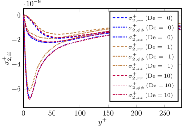
Figure 1: Diagonal components of the polymer and fiber stress tensor.

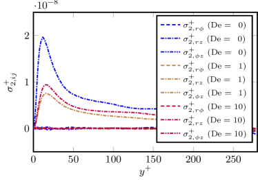
Figure 2: Off-diagonal components of the polymer stress tensor.

In Figures 1 and 2 the diagonal and off-diagonal components of the polymer and fiber stress tensor, $\sigma_{2}$, are shown as functions of the dimensionless distance from the wall. Taking the difference in coordinate systems into consideration, the different components of the stress tensor are in agreement with literature Gillissen et al. (2007b). It can be observed that dumbbells with Deborah number $\text{De}=0$ have the largest, $\text{De}=10$ the second largest, and $\text{De}=1$ the smallest stress tensor components. This is consistent with the results of Virk (1975b), who found that for low concentrations in the onset regime rod-like polyelectrolytes have a stronger drag reducing effect than coiled polyelectrolytes with the same molecular weight. In addition, the behavior of the polymer stress tensors is also as expected, because the dumbbell with $\text{De}=1$ was parameterized to be the dumbbell at which drag reduction onset occurs, and thus polymer stresses are the weakest. Comparing the stress tensor for $\text{De}=0$ with the other two stress tensors for $\text{De}=1$ and $\text{De}=10$, it can be seen that, apart from different values for the maxima and minima, the different stress tensor components have exactly the same shape. Since the stress tensor describes the full interaction of the dumbbells with the solvent, this suggests that the polymers and fibers share the same drag reducing mechanism in the drag reduction onset regime. In addition, since the elastic theory does not apply to fibers, it can be concluded that drag reduction is a local phenomenon and is caused by viscous effects. This is in agreement with Gillissen et al. (2007b). After recognizing that the r axis points to the wall while the y axis points out of the wall, and considering whether the forces are on the beads or on the solvent, our results of the stress tensor are completely consistent with Fig.3 of Gillissen et al. (2007b). On the other hand, our results are different from L’vov et al. (2004) and Benzi et al. (2005). In their work, they use the Doi and Edwards (1986) stress tensor for the fibers and the Giesekus (1962) stress tensors for the elastic polymers. In their analysis they find a coupling between the diagonal and off-diagonal components of the conformation tensor which is linear for elastic polymers and quadradic for rod-like polymers. Benzi et al. (2005) propose a different scaling for the Reynolds stresses at the wall for elastic and rod-like polymers. Since the velocity profile at the wall in $+$ units is expected to be independent of the details of the drag reduction agent Procaccia et al. (2008), this means that the stress tensors for our rigid and elastic dumbbells should show different scaling as well. We do not observe this difference in scaling in our simulations. A possible origin of this difference is that the Giesekus tensor assumes that the polymers are in the Hookean regime (Bird et al., 1987), while in our system the polymers are modeled as Finite Extensible Nonlinear Elastic dumbbells. Another difference is that the work of L’vov et al. (2004) and Benzi et al. (2005) concerns the Maximum Drag Reduction (MDR) regime, while our simulations are in the onset regime. Furthermore, our results show that the stress for rod-like polymers is higher than that for flexible polymers. This is in agreement with Virk (1975b), where polyelectrolyte chains in salt-free conditions (rod-like) and salty conditions (coil-like) were investigated.

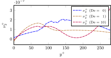
Figure 3: Effective polymer viscosity.

A follow up question that one can ask is where the effective viscosity originates from. Both polymers and fibers are known to show a large increase in viscosity in extensional flow, associated with the diagonal components of the stress tensor (Metzner and Metzner, 1970), but there is also the shear viscosity which is associated with the off-diagonal stress tensor component and rotation. To analyze this question, we evaluate the contribution of the effective viscosity to the momentum balance in its most general form:

$$\nabla\cdot\sigma_{2}=2\nabla\cdot\left(\mathbf{\nu}_{2}\mathbin{:}\mathbf{s}_{1}\right)$$ (8)

with $\mathbf{s}_{1}=1/2({\nabla\mathbf{u}_{1}}^{T}+\nabla\mathbf{u}_{1})$ the rate-of-strain tensor, and $\mathbf{\nu}_{2}$ the fourth order viscosity tensor. Performing a Reynolds decomposition on this equation and taking into account the symmetries of our system gives:

$$\nabla\cdot\sigma_{2}=\nabla\cdot\left[\tilde{\nu}_{2}(r)\frac{\partial\left<w_{1}\right>}{\partial r}+2\left<\mathbf{\nu}_{2}^{\prime}\mathbin{:}\mathbf{s}_{1}^{\prime}\right>\right].$$ (9)

Here ^′ denotes the fluctuating part and $\left<\right>$ the average with:

$$\tilde{\nu}_{2}(r)=\left[\begin{array}[]{ccc}\tilde{\nu}_{2,rr}(r)&0&\tilde{\nu}_{2,zr}(r)\\ 0&\tilde{\nu}_{2,\theta\theta}(r)&0\\ \tilde{\nu}_{2,zr}(r)&0&\tilde{\nu}_{2,zz}(r)\end{array}\right].$$ (10)

Further expanding the above equation gives the following contributions to the Navier-Stokes equations:

$$\left(\nabla\cdot\sigma_{2}\right)_{r} =\frac{1}{r}\frac{\partial}{\partial r}\left[r\tilde{\nu}_{2,rr}(r)\frac{\partial\left<w_{1}\right>}{\partial r}\right]-\frac{\tilde{\nu}_{2,\theta\theta}(r)}{r}\frac{\partial\left<w_{1}\right>}{\partial r} +2\left(\nabla\cdot\left<\mathbf{\nu}_{2}^{\prime}\mathbin{:}\mathbf{s}_{1}^{\prime}\right>\right)_{r}$$ (11)

$$\left(\nabla\cdot\sigma_{2}\right)_{\theta} =\phantom{a} +2\left(\nabla\cdot\left<\mathbf{\nu}_{2}^{\prime}\mathbin{:}\mathbf{s}_{1}^{\prime}\right>\right)_{\theta}$$ (12)

$$\left(\nabla\cdot\sigma_{2}\right)_{z} =\frac{1}{r}\frac{\partial}{\partial r}\left[r\tilde{\nu}_{2,zr}(r)\frac{\partial\left<w_{1}\right>}{\partial r}\right] +2\left(\nabla\cdot\left<\mathbf{\nu}_{2}^{\prime}\mathbin{:}\mathbf{s}_{1}^{\prime}\right>\right)_{z}.$$ (13)

These equations show how, in addition to viscosity-velocity correlations, both the diagonal and off-diagonal components of the stress tensor act on the solvent. While it has been shown that at least at the Maximum Drag Reduction limit all components of the polymer stress tensor are coupled L’vov et al. (2005), one can expect that by leaving out different terms in the above equations their contribution to drag reduction can be investigated. Based on work by L’vov et al. (2004) the results of this can already be found in literature (De Angelis et al., 2004; Gillissen et al., 2007b), where the above viscosity tensor is replaced by a scalar viscosity function $\hat{\nu}_{2}(r)$. The contribution to the Navier-Stokes equations can then be written as:

$$\nabla\cdot\sigma_{2}=\nabla\cdot\left(\hat{\nu}_{2}(r)\mathbf{s}_{1}\right),$$ (14)

which, after Reynolds decomposition, gives a contribution of the form:

$$\left(\nabla\cdot\sigma_{2}\right)_{r} =0$$ (15)

$$\left(\nabla\cdot\sigma_{2}\right)_{\theta} =0$$ (16)

$$\left(\nabla\cdot\sigma_{2}\right)_{z} =\frac{1}{r}\frac{\partial}{\partial r}\left[r\hat{\nu}_{2}(r)\frac{\partial\left<w_{1}\right>}{\partial r}\right].$$ (17)

The above equations only contain the off-diagonal shear viscosity component and none of the extensional viscosity or viscosity-velocity fluctuations. Calculating the fiber viscosity function and using this as an input in a new simulation, all the characteristics of the drag reduced flow can be recovered (Gillissen et al., 2007b). De Angelis et al. (2004) showed that a viscosity gradient at the wall is also able to reproduce the characteristics of a polymer drag reduced flow. This means that not only fluctuations can be ignored (Gillissen et al., 2007b), but also shows that the diagonal components of the stress tensor, and thus extensional viscosity, can be neglected.

Figure 3 shows the effective polymer and fiber viscosities calculated from the stress tensor. Their shape of a gradient at the wall and a plateau in the center is consistent with the viscosity profile used by De Angelis et al. (2004).

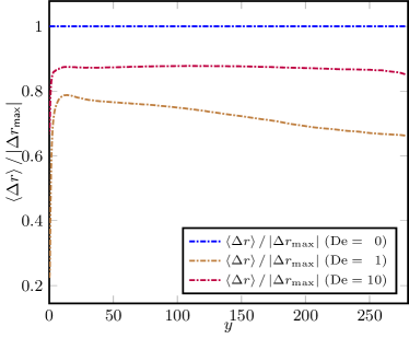
Figure 4: Average relative length of the end-to-end vector of the polymer dumbbells.

To further explore the idea of polymers and fibers creating drag reduction by rotation, the average relative length of the end-to-end vector of all dumbbells normalized by their maximum extensions are shown in Figure 4. Because the molecular weight is kept constant between the different simulations, the maximum extension is $1$ for all cases. The dumbbell with a Deborah number of $\text{De}=0$ is always fully extended. Because it represents the most elastic dumbbell with the longest relaxation time, the dumbbell with a Deborah number of $\text{De}=10$ gets stretched further than the dumbbell with a Deborah number of $\text{De}=1$. This is in agreement with the results shown in Figure 2, which showed that $\text{De}=0$ displays the largest amount of drag reduction followed by Deborah numbers $\text{De}=10$ and $\text{De}=1$. Both elastic dumbbells are stretched the most when close to the wall where gradients are the largest, and relax towards the center of the pipe. That the amount of drag reduction is proportional to the average relative length of the end-to-end vector of the fibers and dumbbells, i.e. their moment arm, and not to the amount of turbulent kinetic energy that can be stored in the backbone, is an additional indication that polymer rotation is essential for drag reduction in the onset regime.

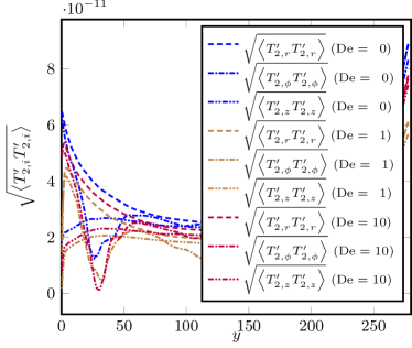
Figure 5: Standard deviation of the torque exerted by the polymer dumbbells on the solvent.

In addition to the end-to-end vector, one can also look into the standard deviation of the torque, which is shown in Figure 5. The torque on the solvent is defined as:

$$T_{2}=-\frac{n}{2V}\left<\Delta\mathbf{x}_{2}\times\Delta{\mathbf{F}_{2}^{h}}\right>$$ (18)

where $n$ is the number of polymer dumbbells in volume $V$, $\Delta\mathbf{x}_{2}=\mathbf{x}_{2,A}-\mathbf{x}_{2,B}$ is the moment arm (i.e. the end-to-end vector), $\Delta{\mathbf{F}_{2}^{h}}={\mathbf{F}_{2,A}^{h}}-{\mathbf{F}_{2,B}^{h}}$, with $\mathbf{F}_{2,i}^{h}$ the hydrodynamic drag force on bead $i$, and $\left<\right>$ indicates an ensemble average. Because of the symmetry of the polymer stress tensor, all components of the torque vector on average are zero. By looking at the standard deviation of the torque, it is possible to gain more insight into polymer/fiber-solvent interactions. Away from the wall the standard deviation of each torque component is about the same for each polymer, indicating that they are freely tumbling around in the bulk. However, as the wall is approached, the different components diverge. The torque has three contributions: i) the length of the moment arm or end-to-end vector, ii) the magnitude of the hydrodynamic forces, and iii) the wall blocking rotation. For the radial component, the wall does not block rotation, and the arm is maximized due to alignment in the streamwise direction. This results in a strong increase of the radial torque fluctuations at the wall. In the streamwise direction, on the other hand, the wall is blocking full rotation, which gives fluctuations which decline monotonically to zero at the wall. For the angular torque fluctuations, the component associated with the shear viscosity, close to the wall rotation is blocked, so the fluctuations go to zero. However, further away from the wall, the maximum moment arm causes a large increase in the torque fluctuations. This shows that, although elasticity is not strictly necessary for drag reduction, the coil-stretch transition is important for polymer drag reduction because it generates a moment arm. Another way of looking at this is that a polymer coil without any stretching can be thought of as a rough sphere which has no drag reducing effect. Fibers, on the other hand, because of their aspect ratio, always have a drag reducing effect. Polymer elasticity allows the roughly spherical coil to stretch into an anisotropic state with an aspect ratio larger than unity. It is not the elasticity that makes a polymer drag-reducing, but the fact that it can transform into anisotropic conformations. This is consistent with the results of Sibilla and Baron (2002) who suggested that shear viscosity cannot be neglected, and Kim et al. (2008), who found that counter-torque by polymers suppresses the formation of hairpin vortices at the wall.

IV Conclusions

To summarize, analyzing the polymer stress tensor it can be observed that polymer and fiber stress tensors show the same characteristics. This indicates that, at least in the low drag reduction regime, polymers and fibers show the same drag reduction mechanism. Because fibers cannot store turbulent kinetic energy in their backbone, this mechanism has to be caused by viscosity effects. We find that the viscous effect arises from rotational motion of fibers and partially stretched flexible chains, which is taken as the unifying drag reduction mechanism in the onset regime. Although viscous effects have been previously attributed to drag reduction in the MDR asymptote regime by L’vov et al. (2004) and Benzi et al. (2005), they have argued that the physical origins of drag reduction by flexible polymers and rigid fibers are different. The difference in scaling between elastic and rod-like polymers suggested by Benzi et al. (2005) is not observed in our simulations. It must be emphasized that the conclusions of Benzi et al. (2005) deal with the regime of maximum drag reduction (MDR) asymptote, whereas our present work is in the onset regime of drag reduction. In addition, Benzi et al. (2005) assume the polymers are in the Hookean regime while our dumbbells are modeled as Finite Extensible Nonlinear Elastic (FENE) springs. Our result in the onset regime is qualitatively different from the arguments in (Procaccia et al., 2008) that for flexible polymers the main source of interaction with turbulent fluctuations is the stretching of polymers by the fluctuating shear and for rod-like polymers dissipation is only taken as the skin friction along the polymer. We find that the molecular rotation is the microscopic mechanism for the onset of drag reduction. By analyzing the different contributions to the effective viscosity tensor, based on work by L’vov et al. (2004), De Angelis et al. (2004), and Gillissen et al. (2007b), it is found that all terms can be neglected except for the off-diagonal component associated with polymer and fiber rotation. To further explore the idea of polymer and fiber rotation being important in the onset of drag reduction regime, polymer and fiber torque fluctuations are investigated. The results suggest that the reason that the coil stretch transition is important for polymer drag reduction is that it generates a moment arm. This is consistent with the results of Kim et al. (2008).

Based on the findings in this work, we propose the rotational orientation time (Kirkwood and Auer, 1951; Muthukumar and Edwards, 1983) as a time criterion for drag reduction.