Derivation and Analysis of Simplified Filters for Complex Dynamical Systems

Abstract

Filtering is concerned with the sequential estimation of the state, and uncertainties, of a Markovian system, given noisy observations. It is particularly difficult to achieve accurate filtering in complex dynamical systems, such as those arising in turbulence, in which effective low-dimensional representation of the desired probability distribution is challenging. Nonetheless recent advances have shown considerable success in filtering based on certain carefully chosen simplifications of the underlying system, which allow closed form filters. This leads to filtering algorithms with significant, but judiciously chosen, model error. The purpose of this article is to analyze the effectiveness of these simplified filters, and to suggest modifications of them which lead to improved filtering in certain time-scale regimes. We employ a Markov switching process for the true signal underlying the data, rather than working with a fully resolved DNS PDE model. Such Markov switching models haven been demonstrated to provide an excellent surrogate test-bed for the turbulent bursting phenomena which make filtering of complex physical models, such as those arising in atmospheric sciences, so challenging.

1 Introduction

1.1 Overview

Filtering is concerned with the sequential updating of Markovian systems, given noisy, partial observations of the system state [29, 30, 37]. Due to the increasing prevalence of data in all areas of science and engineering, and due to the inherent complexity of physical models developed for the description of many phenomena arising in science and engineering, the need for accurate and speedy filters is paramount. However in its full form filtering requires the description of a time-evolving probability distribution on the system state, conditioned on data, which for many systems can be hard to represent in a computationally tractable way. This is a particular challenge for the complex physical models arising in areas such as atmospheric sciences [26], oceanography [2] and oil reservoir simulation [35]. However a recent body of work by Majda and coworkers [21, 31, 30, 8, 27, 7, 6, 38, 22] has demonstrated the possibility of using drastic simplifications of the models for complex turbulent phenomena in order to construct effective filters which are computationally tractable in real-time. The underlying philosophy of this work is to replace the true underlying Markovian model (often deterministic, but chaotic) with a simplified stochastic model which captures the key physical phenomena at the statistical level yet is amenable to closed form expressions for the purpose of filtering. It is possible to interpret this work as providing an important step towards the adoption of physically informed machine learning, going beyond traditional machine learning methodologies which often attempt to build models from the data alone [4, 34]. The purpose of our work is to shed further light on this body of work, through analysis, through the derivation of new methods in the same spirit, and through careful numerical experiments.

In order to carry out this program we do not work with a full complex model of turbulence for our true signal, but rather work with a simple switching stochastic model (SSM), a stochastic differential equation driven by a sign-alternating two-state Markov process [32, 41]. The system is either forced or dissipated depending on the sign of the driving signal, and as a consequence admits intermittent bursting phenomena, similar to what is seen in real turbulent signals [42, 14, 5]. The use of this model as a simplified model for turbulent bursting, and demonstration of its effectiveness in this context, may be seen from the papers [16, 17]. This SSM, then, is viewed as the “true” Markov model whose signals generate the data. Our objective is to find simplified models, amenable to filtering, which capture the essential features of the SSM. We now define the filtering problem and outline the simplified models that we consider.

1.2 The True Model and Model Error

Consider an $\mathbb{R}^{d}$-valued Markov process $x(t)$ where $t\geq 0$. The process is hidden and we only have access to $y_{n}$, $n\in\mathbb{N}$, which is a (partial) noisy observation of $x_{n}\equiv x(nT)$ for some $T>0$. For $Y_{n}:=\{y_{1},\cdots,y_{n}\}$ the key objective in probabilistic filtering is the sequential updating of $\mathbb{P}(x_{n}|Y_{n})$ [28, 23, 1, 12, 30].

To perform filtering, the standard approach adopted in large scale geophysical applications is to alternate the uncertainty propagation $\mathbb{P}\left(x_{n-1}|Y_{n-1}\right)\mapsto\mathbb{P}\left(x_{n}|Y_{n-1}\right)$, and the data acquisition $\mathbb{P}\left(x_{n}|Y_{n-1}\right)\mapsto\mathbb{P}\left(x_{n}|Y_{n}\right)$ in a sequential manner. The former step corresponds to probabilistic solution of the governing equation for $x(t)$, while the latter step is accomplished by Bayes’ rule $\mathbb{P}(x_{n}|Y_{n})\propto\mathbb{P}(x_{n}|Y_{n-1})\mathbb{P}(y_{n}|x_{n})$, which asserts that the posterior distribution is proportional to the product of the prior distribution and the likelihood (viewed as function of $x_{n}$). Examples of Bayesian filters include the Kalman filter [24, 25], the extended Kalman filter [15], the ensemble Kalman filter [13], the particle filter [20] and the Gaussian mixture filter [39, 9, 40].

In this paper the true model $x_{n}$ underlying the data will be found from discrete time sampling of the following switching stochastic model, or SSM for short:

$$\begin{split}\textbf{(SSM)}\qquad\begin{cases}du&=-\gamma udt+\sigma_{u}dB_{u}\\ \gamma&\in\,\,\,\{\gamma_{+},\gamma_{-}\}\end{cases}\end{split}$$ (1.1)

where $\gamma(t)$ is a Markov process, alternately taking constant values of $\{\gamma_{+}>0,\gamma_{-}<0\}$. The distribution functions of the random variables

$$\begin{split}\tau^{\gamma_{+}}&=\inf\{t:\gamma(t)=\gamma_{-}|\gamma(0)=\gamma_{+}\}\\ \tau^{\gamma_{-}}&=\inf\{t:\gamma(t)=\gamma_{+}|\gamma(0)=\gamma_{-}\}\end{split}$$

are given by

$$\begin{split}\mathbb{P}(\tau^{\gamma_{+}}<t)&=1-e^{-\frac{\lambda_{+}}{\epsilon}t}\\ \mathbb{P}(\tau^{\gamma_{-}}<t)&=1-e^{-\frac{\lambda_{-}}{\epsilon}t}\end{split}$$

respectively. The positive parameter $\epsilon$ determines the transition rates, accounting for the time-scale separation between input signal $\gamma$ and output response $u$. In case of small $\epsilon$, there is rapid switching between $\gamma_{+}$ and $\gamma_{-}$. On the other hand, switching is a rare event when $\epsilon$ is large. In the general notation above we have $x=(u,\gamma).$

For $x_{n}=(u_{n},\gamma_{n})=(u(nT),\gamma(nT))$ we assume the noisy observations are of the form

$$\qquad y_{n}=u_{n}+\eta_{n},\qquad\eta_{n}\sim\mathcal{N}({0},R_{n})$$ (1.2)

where $\{\eta_{n}\}_{n\geq 0}$ is an independent and identically distributed centred Gaussian. The filtering distribution $\mathbb{P}(x_{n}|Y_{n})$, determined by (1.1) and (1.2), does not allow for a closed-form representation. In the following, we address the problem through filtering with model error: that is, instead of a straightforward application to the genuine system, we replace the process $x$ by a different Markov model which is more amenable to filtering explicitly than is the SSM. We tune the parameters of the new models to maximize their statistical resemblances with the SSM. It is important to note that in this paper, due to the low dimensionality of SSM, the introduction of reduced models used for filtering presumably does not lead to a significant saving of computational costs. However the aim is to understand the application of the methodology developed by Majda and coworkers which is targetted at situations where the true signal is very expensive to simulate, whilst the models used for filtering are orders of magnitude cheaper. Furthermore we investigate a new theory-based conceptual framework to illustrate this body of work, and to develop generalizations of it, working in a simple setting where the true signal of interest comes from the SSM.

There are four forms of filters with model error considered in this paper (acronyms explained later). The MSM and DSM are particularly relevant when $\epsilon$ is smaller, while the dMSM and dDSM are designed especially for larger $\epsilon$. The MSM is found from the SSM by replacing the switching process $\gamma$ by its mean (constant in time) value, giving rise to a process ${\bar{u}}$ instead of $u$. The DSM is found by replacing the switching process $\gamma$ by the solution of an Ornstein-Uhlenbeck (OU) process, giving rise to a process ${\widehat{u}}$ instead of $u.$ The dMSM is found by replacing $u$ by a process with a constant $\gamma$ in time, but choosing that constant randomly, according to carefully chosen weights. This leads to replacement of $u$ by a process ${\bar{u}}^{\prime}.$ And finally the dDSM is found by replacing $u$ by ${\widehat{u}}^{\prime}$ in which $\gamma$ is given by one of two OU processes for all time, but choosing the OU process randomly, according to carefully chosen weights. From now on, it will help to keep in mind that MSM and DSM are approximations of SSM for smaller $\epsilon$, and dMSM and dDSM are approximations of SSM for larger $\epsilon$.

1.3 Our Contributions

Existing and extensive numerical studies naturally give rise to two fundamental questions about filtering with model error: (i) what are the precise conditions under which a given filter with model error is the best choice out of some class of filters; and (ii) how to choose the free parameters so as to maximize the consequent filtering accuracy. To address these questions we investigate the accuracy of the filters with model error via careful numerical experiments, and introduce a systematic approach for parameter determination. Specifically, our contributions in the present paper are as follows:

• in addition to studying the filters with model error MSM and DSM, introduced in [16, 17], we also introduce our own filters with model error: dMSM and dDSM;

• we build a Gaussian filter and a Gaussian mixture filter for SSM;

• we show the consistency of the reduced models in the extremely small (large) $\epsilon$ regime by proving limit theorems that connect the filter signal models MSM (dMSM) and DSM (dDSM) with the true signal model SSM;

• we use asymptotic analysis in the small (large) $\epsilon$ regime to obtain analytic formulae for the adaptive parameters of the simplified models MSM (dMSM) and DSM (dDSM);

• we employ optimization to solve minimization problem that yields suitable parameters for the simplifications when the scale-separation is not extreme but moderate or weak;

• we perform direct numerical simulations to show the accuracy and feasibility of the methods.

1.4 Organization of the Paper

The paper is organized as follows. We precisely define the models used for filtering in section 2. Our main results are in section 3, where various tools, tuned to the relevant parameter regime for $\epsilon$, are deployed to improve filtering accuracy. We perform numerical experiments in section 4 and draw conclusions in section 5. Lengthy calculations concerning the analysis of models are gathered in the appendices, in order to improve accessibility of the paper.

2 Filtering With Model Error: Simplifications of SSM

Here we define four adaptive approximate models for SSM, based on the analysis of the qualitative behaviors of the switching process, and use them to build filters. Subsection 2.1 is concerned with the case when $\epsilon$ is small (scale-separation regime) and subsection 2.2 is when $\epsilon$ is large (rare-event regime).

2.1 Scale-Separation Regime

2.1.1 Mean Stochastic Model (MSM)

In many multi-scale problems, the governing equation in which the driving signal is significantly faster is replaced by an equation with non-oscillatory coefficient found as a limit (usually in a weak sense) of scale-separation [36, 3, 10]. This work suggests that, when $\epsilon$ is sufficiently small, the mean stochastic model (MSM)

$$\begin{split}\textbf{(MSM)}\qquad\left\{\begin{array}[]{ll}d\bar{u}&=-\bar{\gamma}\bar{u}\,dt+\sigma_{u}dB_{u}\\ \bar{\gamma}&=\text{const}\end{array}\right.\end{split}$$ (2.3)

can be a good approximation of SSM. Using MSM for filtering we note that, provided $\bar{u}_{0}$ is Gaussian, all distributions $\mathbb{P}(\bar{u}_{n-1}|Y_{n-1})\mapsto\mathbb{P}(\bar{u}_{n}|Y_{n-1})\mapsto\mathbb{P}(\bar{u}_{n}|Y_{n})$ are Gaussians and may be updated by the Kalman filter [24].

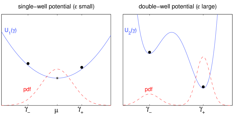
Figure 1: Regularized modeling of the qualitative behaviors of switching process.

2.1.2 Diffusive Stochastic Model (DSM)

The diffusive stochastic model (DSM) is given by

$$\begin{split}\textbf{(DSM)}\qquad\left\{\begin{array}[]{ll}d\widehat{u}&=-\widehat{\gamma}\widehat{u}\,dt+\sigma_{u}dB_{u}\\ d\widehat{\gamma}&=-\frac{\nu}{\epsilon}(\widehat{\gamma}-\mu)\,dt+\frac{\sigma}{\sqrt{\epsilon}}dB_{\gamma}\\ \end{array}\right.\end{split}$$

Note that $\widehat{\gamma}$ is in an Ornstein-Uhlenbeck process: solution of the Langevin equation

$$\begin{split}d{\widetilde{\gamma}}&=-\frac{1}{\epsilon}\nabla U({\widetilde{\gamma}})dt+\frac{\sigma}{\sqrt{\epsilon}}dB_{\gamma}\end{split}$$ (2.4)

with the potential

$$\begin{split}U(x)=U_{1}(x):=\frac{\nu}{2}(x-\mu)^{2}.\end{split}$$ (2.5)

We aim to tune this process to match the response of the system, in the observed variable $u$. The reason for interest in this model is that, although exact filtering is not possible, it is possible to compute an approximate Gaussian filter, based on exact propagation of the first two moments. Indeed provided $(\widehat{u}(0),\widehat{\gamma}(0))$ is joint Gaussian, the mean and covariance of $(\widehat{u}(T),\widehat{\gamma}(T))$ are exactly solvable. Denoting $\widehat{\gamma}_{n}\equiv\widehat{\gamma}(nT)$, the resultant moment mapping can be used for uncertainty propagation: $\mathbb{P}(\widehat{u}_{n-1},\widehat{\gamma}_{n-1}|Y_{n-1})\mapsto\mathbb{P}(\widehat{u}_{n},\widehat{\gamma}_{n}|Y_{n-1})$. Under this Gaussian approximation, the Kalman filter may be applied to obtain $\mathbb{P}(\widehat{u}_{n},\widehat{\gamma}_{n}|Y_{n-1})\mapsto\mathbb{P}(\widehat{u}_{n},\widehat{\gamma}_{n}|Y_{n})$. The resulting filter is named the stochastic parametrization extended Kalman filter (SPEKF) in [18] where it was introduced. Finally, a proper marginalization at every step yields the object of interest: $\mathbb{P}(\widehat{u}_{n}|Y_{n})$.

2.2 Rare-Event Regime

2.2.1 Dual-mode Mean Stochastic Model (dMSM)

When $\epsilon$ is large enough, transitions in $\gamma$ are rare. To study this case, we build the following dual-mode mean stochastic model (dMSM):

$$\begin{split}\textbf{(dMSM)}\qquad\left\{\begin{array}[]{ll}d\bar{{u}}^{\prime}&=-\bar{{\gamma}}^{\prime}\bar{{u}}^{\prime}\,dt+\sigma_{u}dB_{u}\\ \bar{{\gamma}}^{\prime}&=\left\{\begin{array}[]{ll}{\gamma}_{+}\;\text{with probability}\;\bar{\rho}_{+}\;\text{for}\;t\geq 0\\ {\gamma}_{-}\;\text{with probability}\;\bar{\rho}_{-}=1-\bar{\rho}_{+}\;\text{for}\;t\geq 0\\ \end{array}\right.\end{array}\right.\end{split}$$ (2.6)

as the reduced modeling of SSM. This can be viewed as an example of the more general switching linear dynamical system model [19].

If the probability distribution of $\bar{u}^{\prime}(0)$ is the sum of weighted Gaussian kernels, then note that

$$\begin{split}\mathbb{P}(\bar{u}^{\prime}(T))=\mathbb{P}(\bar{\gamma}^{\prime}=\gamma_{+})\mathbb{P}(\bar{u}^{\prime}(T)|\bar{\gamma}^{\prime}=\gamma_{+})+\mathbb{P}(\bar{\gamma}^{\prime}=\gamma_{-})\mathbb{P}(\bar{u}^{\prime}(T)|\bar{\gamma}^{\prime}=\gamma_{-}).\end{split}$$ (2.7)

Under this assumption on $\bar{u}^{\prime}(0)$, then, we may use the Gaussian mixture filter to obtain the exact filtering solution of dMSM. The procedure $\mathbb{P}(\bar{u}^{\prime}_{n-1}|Y_{n-1})\mapsto\mathbb{P}(\bar{u}^{\prime}_{n}|Y_{n-1})$ is performed using (2.7), and a parallel application of the Kalman filter to each Gaussian kernel, along with updating of the weights of each kernel, completes the update $\mathbb{P}(\bar{u}^{\prime}_{n}|Y_{n-1})\mapsto\mathbb{P}(\bar{u}^{\prime}_{n}|Y_{n})$.

In practice, the geometric growth in the number of kernels in the number of prediction steps prevents tractable exact inference as data is accumulated sequentially. One resolution that we adopt here is through the projection of the filtering solution onto the space of tractable distributions. Following the idea of assumed density filtering [33], a large mixture of Gaussians is replaced by a smaller mixture of Gaussians at regular time-intervals, while filtering progresses [11].

2.2.2 Dual-mode Diffusive Stochastic Model (dDSM)

As in the DSM we now try to use a diffusion process to model the switching process $\gamma$, in order to benefit from the possibility of propagating second moments exactly, as is done in the DSM. When $\epsilon$ is large, however, the process (2.4) with the single-well potential (2.5) is not suitable for mimicking rare transitions. We instead consider a double-well potential $U_{2}(x)$ for $U(x)$ (illustrated in the right-panel of Fig. 1). In this scenario, the motion of $\widetilde{\gamma}$ is captured within either of the potential wells for significant time periods, but random perturbations allow it to effectively jump over the potential barrier and enter the parallel metastable state.

Based upon the quadratic expansions

$$\begin{split}U_{2}(x)&\simeq\left\{\begin{array}[]{ll}U_{2}(\mu_{+})+\frac{\nu_{+}}{2}(x-\mu_{+})^{2}\qquad\text{when}\;\;|x-\mu_{+}|\;\;\text{is small}\\ U_{2}(\mu_{-})+\frac{\nu_{-}}{2}(x-\mu_{-})^{2}\qquad\text{when}\;\;|x-\mu_{-}|\;\;\text{is small}\\ \end{array}\right.\end{split}$$

we build a new model

$$\begin{split}\textbf{(dDSM)}\qquad\left\{\begin{array}[]{ll}d\widehat{{u}}^{\prime}&=-\widehat{{\gamma}}^{\prime}\widehat{{u}}^{\prime}\,dt+\sigma_{u}dB_{u}\\ d\widehat{{\gamma}}^{\prime}&=\left\{\begin{array}[]{ll}-\frac{\nu_{+}}{\epsilon}(\widehat{{\gamma}}^{\prime}-\mu_{+})\,dt+\frac{\sigma_{+}}{\sqrt{\epsilon}}dB_{\gamma}\;\text{with probability}\;\widehat{\rho}_{+}\\ -\frac{\nu_{-}}{\epsilon}(\widehat{{\gamma}}^{\prime}-\mu_{-})\,dt+\frac{\sigma_{-}}{\sqrt{\epsilon}}dB_{\gamma}\;\text{with probability}\;\widehat{\rho}_{-}=1-\widehat{\rho}_{+}\end{array}\right.\end{array}\right.\end{split}$$ (2.8)

where the uncertainty is separately delivered by two independent sets of SDEs. Eq. (2.8) is named by the dual-mode diffusive stochastic model (dDSM).

When $(\widehat{u}^{\prime}(0),\widehat{\gamma}^{\prime}(0))$ is a Gaussian mixture, utilizing the exact solvability of the first two moments of the propagated distributions (as for DSM), the probability of $(\widehat{u}^{\prime}(T),\widehat{\gamma}^{\prime}(T))$ can be approximated as Gaussian mixture with the number of kernels doubled, similarly to dMSM. As for dMSM we may perform a reduction of the number of mixtures to retain computational tractability. In this way, the approximate Gaussian mixture filter $\mathbb{P}(\widehat{u}^{\prime}_{n-1},\widehat{\gamma}^{\prime}_{n-1}|Y_{n-1})\mapsto\mathbb{P}(\widehat{u}^{\prime}_{n},\widehat{\gamma}^{\prime}_{n}|Y_{n-1})\mapsto\mathbb{P}(\widehat{u}^{\prime}_{n},\widehat{\gamma}^{\prime}_{n}|Y_{n})$ is established.

3 Model Validations

In this section, we proceed (i) to validate the proposed models, and (ii) to determine the adaptive parameters. We classify the $\epsilon$ parameter regime into the six regions; the scale-separation limit $\{\epsilon\to 0\}$, the sharp scale-separation regime $\{\epsilon\ll 1\}$, the imprecise scale-separation regime $\{\epsilon<1\}$, the moderately rare-event regime $\{\epsilon>1\}$, the extremely rare-event regime $\{\epsilon\gg 1\}$, the rare-event limit $\{\epsilon\to\infty\}$. Subsection 3.1 is devoted to the study of the case $\{\epsilon\to 0,\epsilon\to\infty\}$, and subsection 3.2 to $\{\epsilon\ll 1,\epsilon\gg 1\}$, and subsection 3.3 to $\{\epsilon<1,\epsilon>1\}$.

3.1 Convergence Results

Here we demonstrate the consistency of the simplified models by showing that $u_{T},\widehat{u}_{T}\to\bar{u}_{T}$ (subscript notation will be abused and $u_{T}=u(T)$) as $\epsilon\to 0$ and that $u_{T},\widehat{u}^{\prime}_{T}\to\bar{u}^{\prime}_{T}$ as $\epsilon\to\infty$ in senses elucidated in what follows. All proofs are deferred to the Appendix C.

3.1.1 Scale-Separation Limit

The main results here are the following theorem and corollary; the constants are defined in the developments following their statements.

Theorem 3.1

Assume that ${u}_{0}$, $\bar{u}_{0}$ and $\widehat{u}_{0}$ are identically distributed Gaussian random variables, and assume that $({u}_{0},{\gamma}_{0})$ and $(\widehat{u}_{0},\widehat{\gamma}_{0})$ are independent pairs of random variables. If $\bar{\gamma}$ and $\mu$ are equal to $\bar{\gamma}_{\infty}\equiv\frac{\lambda_{-}\gamma_{+}+\lambda_{+}\gamma_{-}}{\lambda_{-}+\lambda_{+}}$, then, for any fixed $T>0$, as $\epsilon\to 0$ the mean and variance of $u_{T}$ and $\widehat{u}_{T}$ converge to those of $\bar{u}_{T}$.

Proof 3.1 (of Theorem 3.1).

This follows from Lemmas 3.1, 3.2, 3.3, using the explicit calculations which are presented after the corollary below.

Corollary 3.1

Under the conditions in Theorem 3.1, the mean and variance in the Gaussian filters for $u_{n}|Y_{n}$ (defined in Appendix A.3.1) and $\widehat{u}_{n}|Y_{n}$, converge to those of $\bar{u}_{n}|Y_{n}$, for fixed $n>0$, as $\epsilon\to 0$.

Proof 3.2 (of Corollary 3.1).

This follows from the data assimilation formula of the Kalman filter [1].

Let ${u}^{\epsilon}$ solve

$$\begin{split}d{u}^{\epsilon}&=-{\gamma}^{\epsilon}{u}^{\epsilon}dt+\sigma_{u}dB_{u}\end{split}$$ (3.9)

for a random process ${\gamma}^{\epsilon}$. For $\Gamma^{\epsilon}_{t}\equiv\int^{t}_{0}{\gamma}^{\epsilon}(s)ds$ the integral process of ${\gamma}^{\epsilon}$ we have the variation-of-constants yields

$$\begin{split}u_{T}^{\epsilon}&=e^{-\Gamma^{\epsilon}_{T}}u_{0}^{\epsilon}+\sigma_{u}\int^{T}_{0}e^{-(\Gamma^{\epsilon}_{T}-\Gamma^{\epsilon}_{t})}dB_{u}(t).\end{split}$$ (3.10)

Application of the Itô formula shows that the mean and covariance are given by

$$\begin{split}\left\langle{u}^{\epsilon}_{T}\right\rangle&=\left\langle e^{-{\Gamma}^{\epsilon}_{T}}{u}^{\epsilon}_{0}\right\rangle\\ \text{Var}(u^{\epsilon}_{T})&=\left\langle\left(e^{-{\Gamma}^{\epsilon}_{T}}u_{0}^{\epsilon}\right)^{2}\right\rangle-\left\langle e^{-{\Gamma}^{\epsilon}_{T}}u^{\epsilon}_{0}\right\rangle^{2}+\sigma_{u}^{2}\int^{T}_{0}\left\langle e^{-2({\Gamma}^{\epsilon}_{T}-{\Gamma}^{\epsilon}_{t})}\right\rangle dt.\end{split}$$ (3.11)

Here and henceforth, $\langle\cdots\rangle$ denotes the statistical average. Eq. (3.11) reveals that the moment generating function (MGF) of integral process of $\gamma^{\epsilon}$ are particularly relevant to the first two moments propagation of $u^{\epsilon}$ governed by (3.9).

Lemma 3.1

Let $\bar{u}_{t}$ satisfy MSM (2.3). If

$$\left\langle e^{\alpha(\Gamma^{\epsilon}_{T}-\Gamma^{\epsilon}_{t})}\right\rangle\to e^{\alpha\bar{\gamma}(T-t)}\quad\text{for}\;\;\;\alpha=-1,-2\;\;\;\text{and}\;\;\;0\leq t\leq T$$ (3.12)

and if

$$\begin{split}\left\langle\left(e^{-{\Gamma}^{\epsilon}_{T}}u_{0}^{\epsilon}\right)^{m}\right\rangle\to\left\langle\left(e^{-\bar{\gamma}T}\bar{u}_{0}\right)^{m}\right\rangle\quad\text{for}\;\;\;m=1,2\end{split}$$ (3.13)

as $\epsilon\to 0$ then the mean and variance of ${u}^{\epsilon}_{T}$ converge to those of $\bar{u}_{T}$. Further if

$$\begin{split}\left\langle\left(e^{-\Gamma^{\epsilon}_{T}}{u}^{\epsilon}_{0}-e^{-\bar{\gamma}T}\bar{u}_{0}\right)^{2}\right\rangle\to 0\end{split}$$ (3.14)

as $\epsilon\to 0$ then ${u}^{\epsilon}_{T}$ converges to $\bar{u}_{T}$ in $L^{2}(\Omega;{\mathbb{R}}).$ The convergence rates are determined by those associated with Eqs. (3.12), (3.13) and (3.14).

Let $\Gamma_{t}\equiv\int^{t}_{0}\gamma(s)ds$ and $\widehat{\Gamma}_{t}\equiv\int^{t}_{0}\widehat{\gamma}(s)ds$ be the integral processes associated to SSM and DSM respectively. Because $\bar{\Gamma}_{t}\equiv\int_{0}^{t}\bar{{\gamma}}(s)ds=\bar{{\gamma}}t$ ($\bar{{\gamma}}(s)=\bar{{\gamma}}$ is constant) in the case of the MSM, we expect $u_{T},\widehat{u}_{T}\to\bar{u}_{T}$ provided both integral processes, $\Gamma_{t}$ and $\widehat{\Gamma}_{t}$, behave like the probability distribution $\delta_{\bar{\gamma}t}$ in the small $\epsilon$ limit. It turns out this is indeed the case due to averaging. The next two lemmas highlight this behavior.

Lemma 3.2 (SSM)

Let $\gamma_{t}\sim\rho_{+}(t)\delta_{\gamma_{+}}+\rho_{-}(t)\delta_{\gamma_{-}}$ then, for any fixed $t>0$, $\rho_{\pm}(t)\to\frac{\lambda_{\mp}}{\lambda_{-}+\lambda_{+}}$ as $\epsilon\to 0$. Let $\gamma_{\infty}\sim\frac{\lambda_{-}}{\lambda_{-}+\lambda_{+}}\delta_{\gamma_{+}}+\frac{\lambda_{+}}{\lambda_{-}+\lambda_{+}}\delta_{\gamma_{-}}$ and $\bar{\gamma}_{\infty}\equiv\langle\gamma_{\infty}\rangle=\frac{\lambda_{-}\gamma_{+}+\lambda_{+}\gamma_{-}}{\lambda_{-}+\lambda_{+}}$ then, for any fixed $T>t>0$, we have $\left\langle e^{\alpha({\Gamma}_{T}-{\Gamma}_{t})}\right\rangle\to e^{\alpha\bar{\gamma}_{\infty}(T-t)}$ as $\epsilon\to 0$.

Lemma 3.3 (DSM)

Let $\widehat{\gamma}_{\infty}\sim\mathcal{N}(\mu,\sigma^{2}/2\nu)$ then, for any fixed $t>0$, the mean and variance of $\widehat{\gamma}_{t}$ converge to those of $\widehat{\gamma}_{\infty}$ as $\epsilon\to 0$. Furthermore, we have, for any fixed $T>t>0$, $\left\langle e^{\alpha(\widehat{\Gamma}_{T}-\widehat{\Gamma}_{t})}\right\rangle\to e^{\alpha\mu(T-t)}$ as $\epsilon\to 0$.

3.1.2 Rare-Event Limit

The main results in this regime are the following theorem and corollary.

Theorem 3.2

Assume that ${u}_{0}$, $\bar{u}^{\prime}_{0}$ and $\widehat{u}^{\prime}_{0}$ are identically distributed Gaussian random variables, and assume that $({u}_{0},{\gamma}_{0})$ and $(\widehat{u}^{\prime}_{0},\widehat{\gamma}^{\prime}_{0})$ are independent pairs of random variables. Then, for any fixed $T>0$, the mean and variance of $\mathbb{P}({u}_{T}|{\gamma}_{0}=\gamma_{\pm})$, $\mathbb{P}(\widehat{u}^{\prime}_{T}|\widehat{\gamma}^{\prime}_{0}=\gamma_{\pm})$ converges to those of $\mathbb{P}(\bar{u}^{\prime}_{T}|\bar{\gamma}^{\prime}=\gamma_{\pm})$ as $\epsilon\to\infty$.

Furthermore, let ${\gamma}_{0}\triangleq\gamma_{\infty}$, and if $\bar{\gamma}^{\prime}$ and $\widehat{\gamma}^{\prime}_{0}$ are identically distributed with $\gamma_{\infty}$, then the weight, mean and variance of components in the Gaussian mixture approximation for ${u}_{T}$, $\widehat{u}^{\prime}_{T}$ converge to those of $\bar{u}^{\prime}_{T}$ as $\epsilon\to\infty$.

Proof 3.3.

This follows from Lemmas 3.4, 3.5, 3.6 below.

Corollary 3.2

Under the conditions in Theorem 3.2, the weight, mean and variance of mixture components in the Gaussian mixture filters for $u_{n}|Y_{n}$ (defined in Appendix A.3.2) and $\widehat{u}^{\prime}_{n}|Y_{n}$, converge to those of $\bar{u}^{\prime}_{n}|Y_{n}$, for fixed $n>0$, as $\epsilon\to\infty$.

Proof 3.4.

This follows from parallel application of the Kalman filter update to the mixture components.

Lemma 3.4

Let $\bar{u}^{\prime}_{t}$ solve dDSM (2.6). If, for each fixed $T>t>0$,

$$\left\langle e^{\alpha(\Gamma^{\epsilon}_{T}-\Gamma^{\epsilon}_{t})}|\gamma^{\epsilon}_{0}=\gamma_{\pm}\right\rangle\to e^{\alpha{\gamma_{\pm}}(T-t)}\quad\text{for}\;\;\;\alpha=-1,-2\;\;\;\text{and}\;\;\;0\leq t\leq T$$ (3.15)

and if

$$\begin{split}\left\langle\left(e^{-{\Gamma}^{\epsilon}_{T}}u_{0}^{\epsilon}\right)^{m}|\gamma^{\epsilon}_{0}=\gamma_{\pm}\right\rangle\to\left\langle\left(e^{-{\gamma}_{\pm}T}\bar{u}_{0}\right)^{m}\right\rangle\quad\text{for}\;\;\;m=1,2\end{split}$$ (3.16)

as $\epsilon\to\infty,$ then the mean and variance of ${u}^{\epsilon}_{T}|\gamma^{\epsilon}_{0}=\gamma_{\pm}$ converge to those of $\bar{u}_{T}|\bar{\gamma}^{\prime}=\gamma_{\pm}$. The convergence rates are determined by those associated with Eqs. (3.15), (3.16).

Furthermore, if ${\gamma}^{\epsilon}_{0}\triangleq\bar{\gamma}^{\prime}$, then the weight, mean and variance of components in the Gaussian mixture approximation for ${u}^{\epsilon}_{T}$ converge to those of $\bar{u}_{T}$ from $\mathbb{P}({u}^{\epsilon}_{T})=\mathbb{P}({\gamma}^{\epsilon}_{0}=\gamma_{+})\mathbb{P}({u}^{\epsilon}_{T}|{\gamma}^{\epsilon}_{0}=\gamma_{+})+\mathbb{P}({\gamma}^{\epsilon}_{0}=\gamma_{-})\mathbb{P}({u}^{\epsilon}_{T}|{\gamma}^{\epsilon}_{0}=\gamma_{-})$.

To ensure the convergences of SSM and dDSM to dMSM, as $\epsilon$ grows, both ${\Gamma}_{t}$ and $\widehat{\Gamma}^{\prime}_{t}\equiv\int^{t}_{0}\widehat{\gamma}^{\prime}(s)ds$ need to converge to $\bar{\Gamma}^{\prime}_{t}\equiv\int_{0}^{t}\bar{{\gamma}}^{\prime}(s)ds\sim\bar{\rho}_{+}\delta_{\gamma_{+}t}+\bar{\rho}_{-}\delta_{\gamma_{-}t}$.

Lemma 3.5 (SSM)

For fixed $T>t>0$ $\left\langle e^{\alpha(\Gamma_{T}-\Gamma_{t})}|{\gamma}_{0}=\gamma_{\pm}\right\rangle\to e^{\alpha\gamma_{\pm}(T-t)}$ as $\epsilon\to\infty$.

Lemma 3.6 (dDSM)

For fixed $T>t>0$ $\left\langle e^{\alpha(\widehat{\Gamma}^{\prime}_{T}-\widehat{\Gamma}^{\prime}_{t})}|\widehat{\gamma}^{\prime}_{0}=\gamma_{\pm}\right\rangle\to e^{\alpha\gamma_{\pm}(T-t)}$ as $\epsilon\to\infty$.

3.2 Asymptotic Matching

The convergence results in the preceding subsection demonstrate that the filtering performances of the approximate filters, and the exact filter, would be similar to one another in that $\bar{\gamma}=\bar{\gamma}_{\infty}$, $\mu=\bar{\gamma}_{\infty}$ (when $\epsilon\ll 1$) and $\bar{\gamma}^{\prime}\triangleq{\gamma}_{\infty}$, $\widehat{\rho}_{\pm}\propto{\lambda_{\mp}}$, $\mu_{\pm}=\gamma_{\pm}$ (when $\epsilon\gg 1$). The former result relates to the robustness of the DSM filter inherited from the adaptive parameters $\{\mu,\sigma\}$, demonstrated here when $\epsilon$ is small, and demonstrated through extensive numerical simulations in [16, 17].

However, when $\epsilon$ deviates considerably from the two extreme values ($\epsilon=0$ and $\epsilon=\infty$), the choice of associated parameters in the filtering models is indeed one critical factor for a successful filtering with model error. The current and next subsections concern the determination of $\Theta\equiv\{\mu,\nu,\sigma\}$ for DSM, and $\Theta^{\prime}\equiv\{\widehat{\rho}_{\pm},\mu_{\pm},\nu_{\pm},\sigma_{\pm}\}$ for dDSM. Unlike earlier works in this area where these associated parameters are chosen from a number of parallel direct numerical simulations comparing the original dynamics and its simplifications, our approach will specify the parameters in a systematic analysis-based manner.

3.2.1 Sharp Scale-Separation Regime

In this parameter regime, because DSM is associated to a nonlinear approximate Kalman filter, we attempt to equate the first and second order statistics of SSM and DSM,

$$\begin{split}\left\{\begin{array}[]{ll}\langle u_{T}\rangle&=\langle\widehat{u}_{T}\rangle\\ \text{Var}(u_{T})&=\text{Var}(\widehat{u}_{T})\end{array}\right.\end{split}$$ (3.17)

for high accuracy. It is worth noticing that, in view of (3.11), if the MGFs agree with one another, that is if

$$\qquad\;\left\langle e^{\alpha\Gamma_{T}}\right\rangle=\left\langle e^{\alpha\widehat{\Gamma}_{T}}\right\rangle\qquad\quad\text{for}\;\;\;\alpha=-1,-2$$ (3.18a)

$$\left\langle e^{\alpha(\Gamma_{T}-\Gamma_{t})}\right\rangle=\left\langle e^{\alpha(\widehat{\Gamma}_{T}-\widehat{\Gamma}_{t})}\right\rangle\quad\text{for}\;\;\;\alpha=-2\;\;\;\text{and}\;\;\;0\leq t\leq T$$ (3.18b)

and if $({u}_{0},{\gamma}_{0})$ and $(\widehat{u}_{0},\widehat{\gamma}_{0})$ are uncorrelated, and if ${u}_{0}\triangleq\widehat{u}_{0}$, then Eq. (3.17) holds. Motivated by convergence to the common limit, as demonstrated above, we here strive to asymptotically satisfy (3.18b) when $\epsilon\ll 1$.

To that end, we derive the approximation

$$\begin{split}\left\langle e^{\alpha(\Gamma_{T}-\Gamma_{t})}\right\rangle&\simeq\exp\Bigg{(}\alpha\bar{\gamma}_{\infty}(T-t)+\alpha^{2}\frac{3}{8}\frac{(\gamma_{-}-\gamma_{+})^{2}(\lambda_{-}^{2}+\lambda_{+}^{2})}{\lambda_{-}\lambda_{+}(\lambda_{+}+\lambda_{-})}(T-t)\epsilon\\ &+\alpha\left(\mathbb{P}(\gamma_{0}=\gamma_{+})\frac{(\gamma_{+}-\gamma_{-})}{4\lambda_{+}}+\mathbb{P}(\gamma_{0}=\gamma_{-})\frac{(\gamma_{-}-\gamma_{+})}{4\lambda_{-}}\right)\epsilon+\mathcal{O}(\epsilon^{2})\Bigg{)}\quad\epsilon<T-t\end{split}$$ (3.19)

in the Appendix A.2.1. We also derive the approximations

$$\left\langle e^{\alpha\widehat{\Gamma}_{T}}\right\rangle =\exp\left(\alpha\left(\mu T+\langle\widehat{\gamma}_{0}-\mu\rangle\frac{\epsilon}{\nu}\right)+\alpha^{2}\frac{\sigma^{2}}{2\nu^{2}}T\epsilon+\mathcal{O}(\epsilon^{2})\right)\quad\epsilon<T$$ (3.20a)

$$\left\langle e^{\alpha(\widehat{\Gamma}_{T}-\widehat{\Gamma}_{t})}\right\rangle =\exp\left(\alpha\mu(T-t)+\alpha^{2}\frac{\sigma^{2}}{2\nu^{2}}(T-t)\epsilon+\mathcal{O}(\epsilon^{2})\right)\quad\epsilon<t$$ (3.20b)

in the Appendix B.3.1. Importantly, the exponents of MGFs are of the second-order with respect to $\alpha T$ up to $\mathcal{O}(\epsilon)$, indicating that both $\Gamma_{T}$ and $\widehat{\Gamma}_{T}$ are statistically closer to Gaussian in this parameter regime.

From a comparison between (3.19) and (3.20), we realize Eq. (3.18b) is asymptotically met provided $\bar{\gamma}_{\infty}=\mu$ and

$$\begin{split}\frac{3}{8}\frac{(\gamma_{-}-\gamma_{+})^{2}(\lambda_{-}^{2}+\lambda_{+}^{2})}{\lambda_{-}\lambda_{+}(\lambda_{+}+\lambda_{-})}&=\frac{\sigma^{2}}{2\nu^{2}}\end{split}$$ (3.21)

and

$$\begin{split}\mathbb{P}(\gamma_{0}=\gamma_{+})\frac{(\gamma_{+}-\gamma_{-})}{4\lambda_{+}}+\mathbb{P}(\gamma_{0}=\gamma_{-})\frac{(\gamma_{-}-\gamma_{+})}{4\lambda_{-}}=\frac{\langle\widehat{\gamma}_{0}-\mu\rangle}{\nu}.\end{split}$$ (3.22)

Eqs. (3.21), (3.22) can be solved to determine a unique set of $\{\nu,\sigma^{2}\}$ but might result in $\nu<0$ which is unphysical. In order to avoid this possibility, we impose the equivalence between variances of stationary processes $\gamma_{\infty}$ and $\widehat{\gamma}_{\infty}$

$$\begin{split}\frac{\lambda_{+}\lambda_{-}(\gamma_{+}-\gamma_{-})^{2}}{(\lambda_{-}+\lambda_{+})^{2}}&=\frac{\sigma^{2}}{2\nu}\\ \end{split}$$ (3.23)

instead of Eq. (3.22). From Eqs. (3.21) and (3.23), we obtain

$$\begin{split}\Theta_{\text{naive}}\equiv\begin{cases}\mu&=\bar{\gamma}_{\infty}\\ \nu&=\frac{8}{3}\frac{\lambda_{-}^{2}\lambda_{+}^{2}}{(\lambda_{-}+\lambda_{+})(\lambda_{+}^{2}+\lambda_{-}^{2})}\qquad\text{when}\quad\epsilon\ll 1\\ \sigma^{2}&=\frac{16}{3}\frac{\lambda_{-}^{3}\lambda_{+}^{3}(\gamma_{-}-\gamma_{+})^{2}}{(\lambda_{-}+\lambda_{+})^{3}(\lambda_{+}^{2}+\lambda_{-}^{2})}\\ \end{cases}\end{split}$$ (3.24)

which we term the naive set of DSM parameters, valid when $\epsilon\ll 1$.

3.2.2 Extremely Rare-Event Regime

Using a similar argument to that employed in the case of DSM, we set ${\rho}_{\pm}=\widehat{\rho}_{\pm}=\frac{\lambda_{\mp}}{\lambda_{-}+\lambda_{+}}$ and attempt to satisfy

$$\begin{split}\left\{\begin{array}[]{ll}\langle u_{T}|\gamma_{0}=\gamma_{\pm}\rangle&=\langle\widehat{u}_{T}|\widehat{\gamma}^{\prime}_{0}=\gamma_{\pm}\rangle\\ \text{Var}(u_{T}|\gamma_{0}=\gamma_{\pm})&=\text{Var}(\widehat{u}_{T}|\widehat{\gamma}^{\prime}_{0}=\gamma_{\pm})\end{array}\right.\end{split}$$

hence

$$\quad\;\quad\left\langle e^{\alpha\Gamma_{T}}|\gamma_{0}=\gamma_{\pm}\right\rangle=\left\langle e^{\alpha\widehat{\Gamma}^{\prime}_{T}}|\widehat{\gamma}^{\prime}_{0}=\gamma_{\pm}\right\rangle\qquad\text{for}\;\;\alpha=-1,-2$$ (3.25a)

$$\left\langle e^{\alpha(\Gamma_{T}-\Gamma_{t})}|{\gamma}_{0}=\gamma_{\pm}\right\rangle=\left\langle e^{\alpha(\widehat{\Gamma}^{\prime}_{T}-\widehat{\Gamma}^{\prime}_{t})}|\widehat{\gamma}^{\prime}_{0}=\gamma_{\pm}\right\rangle\;\text{for}\;\;\alpha=-2\;\;\text{and}\;\;0\leq t\leq T$$ (3.25b)

for dDSM.

In the case $\epsilon\gg 1$, we derive

$$\begin{split}\left\langle e^{\alpha\Gamma_{T}}|{\gamma}_{0}=\gamma_{\pm}\right\rangle&\simeq\exp\left(\alpha\gamma_{\pm}T-\frac{1}{\epsilon}\lambda_{\pm}T\right)\\ \end{split}$$ (3.26)

in the Appendix A.2.2 and

$$\begin{split}\left\langle e^{\alpha\widehat{\Gamma}^{\prime}_{T}}|\widehat{\gamma}^{\prime}_{0}=\gamma_{\pm}\right\rangle&\simeq\exp\left(\alpha\left({\gamma}_{\pm}T-\frac{1}{2\epsilon}({\gamma}_{\pm}-\mu_{\pm})\nu_{\pm}T^{2}\right)+\frac{\alpha^{2}}{2}\frac{(\sigma_{\pm})^{2}}{3\epsilon}T^{3}\right)\\ \end{split}$$ (3.27)

in the Appendix B.3.2. Note the exponents in (3.26) and (3.27) are of different forms, indicating both ${\Gamma}_{T}$ and $\widehat{\Gamma}^{\prime}_{T}$ are distant from Gaussian in this parameter regime.

Differently from the case of DSM, we here manage to asymptotically satisfy Eq. (3.25a) alone, yielding

$$\begin{split}\Theta^{\prime}_{\text{naive}}\equiv\begin{cases}\widehat{\rho}_{\pm}=\frac{\lambda_{\mp}}{\lambda_{-}+\lambda_{+}}\\ \mu_{\pm}=2T\frac{\lambda_{+}\lambda_{-}(\gamma_{+}-\gamma_{-})^{2}}{(\lambda_{-}+\lambda_{+})^{2}}+\gamma_{\pm}\qquad\text{when}\quad\epsilon\gg 1\\ \nu_{\pm}=\frac{3\lambda_{\pm}}{2T^{2}}\frac{(\lambda_{-}+\lambda_{+})^{2}}{\lambda_{+}\lambda_{-}(\gamma_{+}-\gamma_{-})^{2}}\\ (\sigma_{\pm})^{2}=\frac{3\lambda_{\pm}}{T^{2}}\\ \end{cases}\end{split}$$ (3.28)

which we term the naive set of dDSM parameters, valid when $\epsilon\gg 1$. Unlike Eq. (3.24), due to the dependence on $T$, the set of parameters (3.28) is valid only for fixed-time prediction. The Gaussian mixture from dDSM with $\Theta^{\prime}_{\text{naive}}$ leads to accurate mean approximations but the accuracy of the variance approximation is not guaranteed in view of Eq. (3.11) where integration over $[0,T]$ is involved.

3.3 Minimizing Sum-of-Squares

In the parameter regime $\epsilon\sim O(1)$, due to the absence of small or large parameters allowing for asymptotic analysis, we invoke a minimization principle to determine the set of parameters $\Theta$ and $\Theta^{\prime}$.

3.3.1 Imprecise Scale-Separation Regime

When $\epsilon<1$, we aim to find $\Theta$ which minimizes the sum-of-squares

$$\begin{split}J(\epsilon)\equiv\kappa\big{|}\langle u_{T}\rangle-\langle\widehat{u}_{T}\rangle\big{|}^{2}+\big{|}\text{Var}(u_{T})-\text{Var}(\widehat{u}_{T})\big{|}^{2}\end{split}$$ (3.29)

where $\kappa\geq 0$ is introduced to ensure appropriate scaling of the two terms in the objective function. To be more precise, given $(\widehat{u}_{0},\widehat{\gamma}_{0})$, Eq. (3.29) is an algebraic relation in terms of $\Theta$ once we impose ${u}_{0}:=\widehat{u}_{0}$ and ${\gamma}_{0}:=\gamma_{\infty}$ (see Appendices A and B). Note that a minimizer of $J(\epsilon)$ comes as close as possible to fulfilling Eq. (3.17). It is worth mentioning that, differently from the MFG matching (3.18b) for which $(\widehat{u}_{0},\widehat{\gamma}_{0})$ should be at most weakly correlated for the approach to be valid, the minimization methodology can be used irrespective of their potentially strong correlation.

We identify a (local) minimizer by taking $\Theta_{\text{naive}}$ as an initial starting point, and applying an optimizer such as gradient descent. This minimization can be performed using continuation in $\epsilon$, starting from $\epsilon\ll 1$ where the initial guess will be accurate. Because the solution of this minimization is computed at each assimilation time step we name it dynamic calibration and denote the resulting time-dependent parameters by $\Theta_{\text{dynamic}}$. Of course the key issue in sequential filtering that we are addressing is to maintain an accurate description of the evolving probability distribution with reasonable computational cost. In this context it is impractical to compute $\Theta_{\text{dynamic}}$ at every observation time. In practice, one can take a time average of a range of dynamic calibrations. We refer to this as static calibration and denote the resulting parameter by $\Theta_{\text{static}}$.

3.3.2 Moderately Rare-Event Regime

As for the extremely rare-event regime, we carry out the same procedure for each stable and unstable Gaussian kernel. As for the imprecise scale-separation regime we also minimize an expression analogous to Eq. (3.29) in which the conditioned mean and covariance are used instead. We first find $\Theta^{\prime}_{\text{dynamic}}$ from $\Theta^{\prime}_{\text{naive}}$, and next find $\Theta^{\prime}_{\text{static}}$ from $\Theta^{\prime}_{\text{dynamic}}$. Unlike the method based on matching MGF asymptotics, where the potential inaccuracy of variance approximations are present, this method simultaneously accounts for accuracy in both the mean and covariance approximations.

4 Numerical Simulations

Having obtained three different versions of adaptive parameters (naive set, static calibration, dynamic calibration) for DSM and dDSM, we here investigate the filtering performances of the suggested models using numerical simulations.

Very importantly, one distinguished advantage of the framework we are currently adopting lies in the analytic tractability of the state space model. In Appendix A.1, we derive the closed form solution (when $\lambda_{+}=\lambda_{-}$) and the series solution (when $\lambda_{+}\neq\lambda_{-}$) for MGFs of the SSM integral process. In Appendix A.3, we use them to design the Gaussian filter (suitable when $\epsilon$ is small) and the Gaussian sum filter (suitable when $\epsilon$ is large) for SSM. Those results from the direct filtering of SSM are then to be used as the reference solutions in subsequent experiments. We emphasize that the presence of these reference probability distributions enables very careful examination of filter accuracy in our numerical experiments, beyond measuring the distance between a realization of the truth signal and the mean of an approximate filtering solution and beyond what is seen in most other works concerning the computational evaluations of filters; this in turn gives further depth to our demonstrations.

In all our experiments, we use the following parameter values to specify the SSM truth model: $\sigma_{u}=0.1549$, $\gamma_{+}=2.27$, $\gamma_{-}=-0.04$, $\lambda_{+}=1$ and $\lambda_{-}=2$ (these choices follow those in [16]). Fixing inter-observation time $T=1$, we study the cases of $\epsilon=10^{-1}$, $10^{0}$, $10^{1}$, $10^{2}$. Each one is selected as representative of the parameter regimes: sharp scale-separation, imprecise scale-separation, moderately rare-event, extremely rare-event, in the order given. Since $\mathbb{E}(\tau_{k})=1/r$ for $\tau_{k}\sim\exp(r)$, the reciprocal of $\epsilon$ equals the average number of transitions from the stable mode ($\gamma=\gamma_{+}$) to the unstable mode ($\gamma=\gamma_{-}$) on the unit time interval. As $\lambda_{-}$ is twice $\lambda_{+}$ in this example, the average time spent in the stable mode is twice that spent in the unstable mode.

We take the initial condition of SSM according to $u_{0}\triangleq\mathcal{N}(0.1,0.0016)$ and $\gamma_{0}\triangleq\gamma_{\infty}$, independently from one the other. For MSM (dMSM), we take $\bar{u}_{0}(\bar{u}^{\prime}_{0})\triangleq u_{0}$. We also take $\bar{\gamma}=\bar{\gamma}_{\infty}(=1.5)$ and $\bar{\gamma}^{\prime}\triangleq{\gamma}_{\infty}$. For DSM (dDSM), we take the independent Gaussian $(\widehat{u}_{0},\widehat{\gamma}_{0})$ (or $(\widehat{u}^{\prime}_{0},\widehat{\gamma}^{\prime}_{0})$) where $\widehat{u}_{0}\triangleq u_{0}$ and $\widehat{\gamma}_{0}\triangleq\mathcal{N}(1.2\bar{\gamma}_{\infty},\text{Var}(\gamma_{\infty}))$. We set $\widehat{\rho}^{\pm}(0)=\bar{\rho}_{\pm}$. For the observational process in Eq. (1.2), we use $R_{n}=0.25E$ where $E\equiv\sigma_{u}^{2}/(2\bar{\gamma})$ (in this case the variance of $\bar{u}_{n}|Y_{n}$ is independent of $n$).

4.1 Performances of Simplified Filters

4.1.1 Sharp Scale-Separation Regime

We first study the case of $\epsilon=10^{-1}$. For the implementation of DSM with dynamic calibration, along with $\Theta_{\text{naive}}$ as a starting point, a local minimizer $\Theta_{\text{dynamic}}$ of Eq. (3.29) is solved at every observation time. The choice of $\kappa$ in $J(\epsilon)$ plays a substantial role in this problem. Here and hereafter, the value of $\kappa$ is set to zero for simplicity and consistency of presentations; this allows the prior mean from dynamic and static calibrations to be inaccurate but, in filtering, the posterior is the main object of interest. The time average of these parameters for $1\leq n\leq 50$ is taken as $\Theta_{\text{static}}$.

In addition to DSM filters, we apply Gaussian filters for MSM and SSM. For the latter, due to distinct $\lambda_{\pm}$, we need to truncate the series solution of the MGF. Hereafter, the first $30$ terms of the series solution will be kept as this ensures accuracy by virtue of the fact that $\mathbb{P}(N_{T}>30)<10^{-5}$.

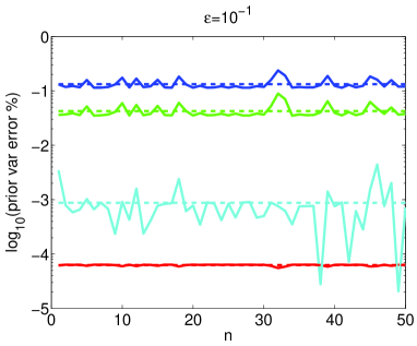
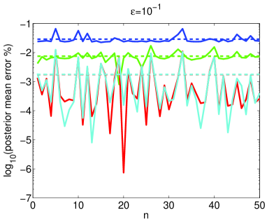
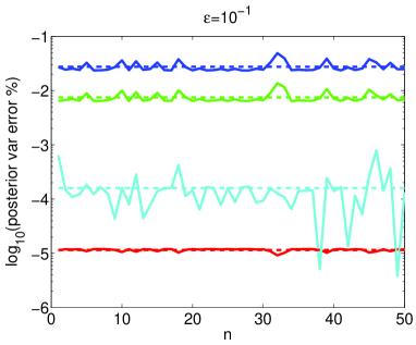
Figure 2: The relative errors of the mean and variance approximations of the prior $u_{n}|Y_{n-1}$ (top) and posterior $u_{n}|Y_{n}$ (bottom) distributions when $\epsilon=10^{-1}$. The dashed lines denote the time averages over $0\leq n\leq 50$.

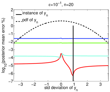
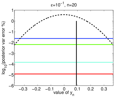
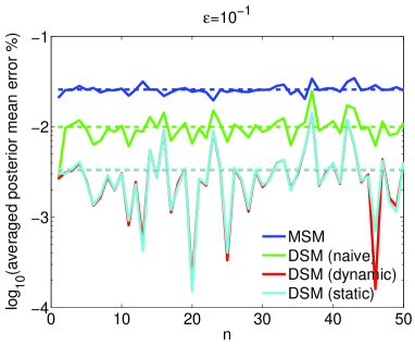
Figure 3: The relative errors of the approximations of the posterior $u_{n}|Y_{n}$ distributions that depend on the realization of $y_{n}=u_{n}+\eta_{n}$ (top and bottom-left), and their statistical averages with respect to the law of $y_{n}$ (bottom-right) when $\epsilon=10^{-1}$. In Gaussian filters, the accuracy of the posterior variance does not depend on the instance of $y_{n}$ (top-right).

In Fig. 3, we depict the relative errors of the prior and posterior approximations in terms of mean and variance. We see that the approximations of DSM with the parameters tuned by our methods are significantly more accurate than the MSM approximation. As expected, the overall errors of the mean and variance relative to those from SSM filtering solution are given in the order : DSM (dynamic calibration) $\lesssim$ DSM (static calibration) $<$ DSM (naive set) $<$ MSM. Admittedly, this result is merely for a single realization of the observation process. However we show that the result is indeed robust with respect to the chosen observational data set in the following manner.

At each observation time step, the posterior distributions of the approximate models are determined by the instance of observation, which is drawn from a Gaussian. In Fig. 3, we depict the dependence of the corresponding filter accuracy on $y_{n}$ for $n=20$ and $n=40$. It is observed that, for most values of $y_{n}$, Gaussian filters for DSM with dynamic and static calibrations significantly outperform MSM, leading to highly accurate posterior approximations. In Fig. 3, we also depict the statistical average of the posterior error with respect to $y_{n}$ for each $n$. There, one can see the ordering of the accuracies is exactly the same as in the single realization experiment.

4.1.2 Imprecise Scale-Separation Regime

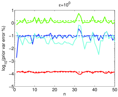
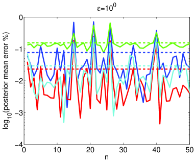
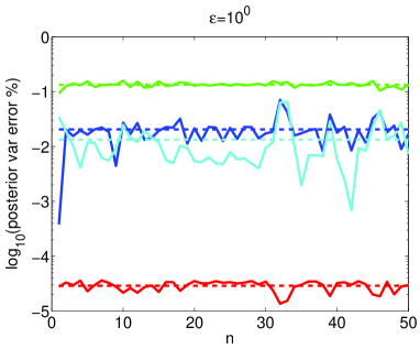
Figure 4: The relative errors of the mean and variance approximations of the prior $u_{n}|Y_{n-1}$ (top) and posterior $u_{n}|Y_{n}$ (bottom) distributions when $\epsilon=10^{0}$.

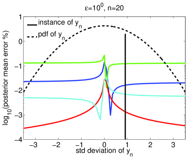
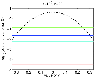
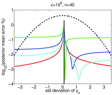
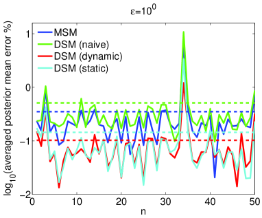
Figure 5: The relative errors of the approximations of the posterior $u_{n}|Y_{n}$ distributions that depend on the realization of $y_{n}=u_{n}+\eta_{n}$, and their statistical averages with respect to the law of $y_{n}$ when $\epsilon=10^{0}$.

Taking $\epsilon=10^{0}$, it is not immediately intuitive whether either the Gaussian description or the Gaussian mixture description is a better approximation of the SSM. It turns out that, in this case, the Gaussian filter for SSM is more suitable as the reference solution; our investigation of this issue can be found in subsection 4.2. Accordingly we find dynamic and static calibrations, and implement Gaussian filters for DSM, MSM and SSM. We depict Fig. 5 and Fig. 5, which correspond, respectively, to Fig. 3 and Fig. 3. The scenario interpreted from the figures is basically the same as the one arising when $\epsilon=10^{-1}$, with one exception that the naive DSM is less accurate than the MSM. This is no surprise, because $\epsilon$ is no longer small and $\Theta_{\text{naive}}$ is no longer expected to be valid. Therefore, the overall errors are ordered as: DSM (dynamic calibration) $\lesssim$ DSM (static calibration) $<$ MSM $<$ DSM (naive set).

4.1.3 Moderately Rare-Event Regime

When $\epsilon=10^{1}$, it is shown in subsection 4.2 that the Gaussian sum filter for SSM, made efficient by merging the mixture approximation of the posterior into a Gaussian at every observation time, is indeed better than the Gaussian filter for the reference solution. We apply the same kind of Gaussian sum filters for dMSM and dDSM. For the dDSM implementations, taking $\Theta^{\prime}_{\text{naive}}$ as a starting point, we solve dynamic calibrations for each of two evolving Gaussian kernels. We then individually average them to obtain a static calibration.

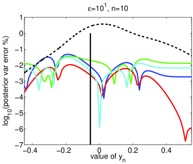
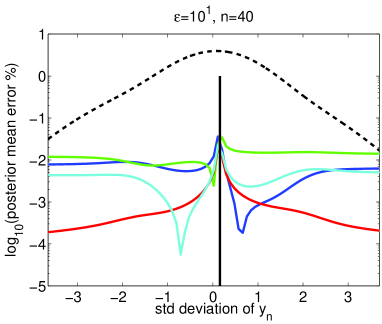
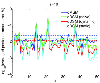
Figure 8: The relative errors of the approximations of the posterior $u_{n}|Y_{n}$ distributions that depend on the realization of $y_{n}=u_{n}+\eta_{n}$, and their statistical averages with respect to the law of $y_{n}$ when $\epsilon=10^{0}$. In Gaussian sum filters, the accuracy of the posterior variance depends on the instance of $y_{n}$ (top-right and middle-right).

In Fig. 7, we depict the relative error for each of the Gaussian kernel approximations. Combining these two cases, we plot Fig. 7 and Fig. 8, which correspond to Fig. 5 and Fig. 5 respectively. Importantly, for comparison, we additionally plot the result from DSM with $(\mu=\bar{\gamma}_{\infty},\nu=0.1\bar{\gamma}_{\infty},\sigma=5\sigma_{u})$. These parameters are the ones used in [16]. They are selected as suitable from direct numerical simulations in this parameter regime, and are interestingly very close to $\Theta_{\text{naive}}$. Here the DSM appears as a reasonable approximation of SSM but this Gaussian filter is characterized by significantly less accuracy than the remaining Gaussian sum filters.

Our simulations further indicate, in this case, that the dependency of filter accuracy on the observation is much more complicated than the previous Gaussian filtering examples (Fig. 8). The overall errors are of the order : dDSM (dynamic calibration) $\lesssim$ dDSM (static calibration) $<$ dMSM $\lesssim$ dDSM (naive set) $<$ DSM (naive set).

4.1.4 Extremely rare-event regime

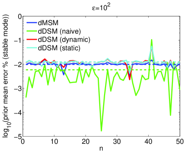
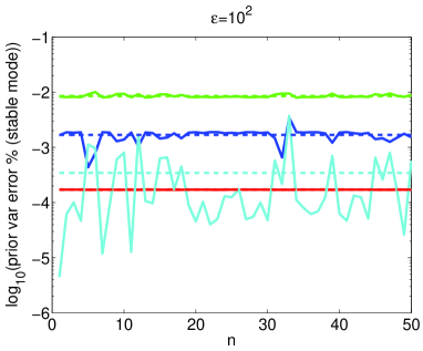
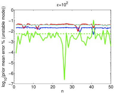
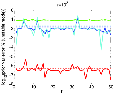
Figure 9: The relative errors of the mean and variance approximations of each Gaussian kernels of the prior distributions when $\epsilon=10^{2}$.

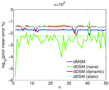
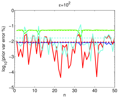
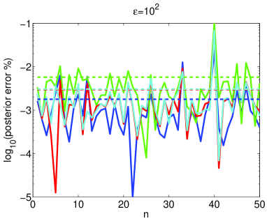
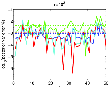
Figure 10: The relative errors of the mean and variance approximations of the prior $u_{n}|Y_{n-1}$ (top) and posterior $u_{n}|Y_{n}$ (bottom) distributions when $\epsilon=10^{2}$.

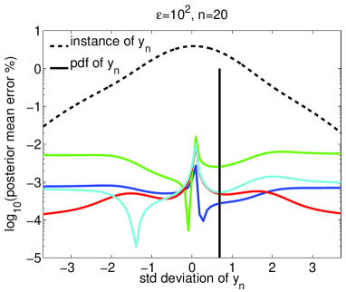
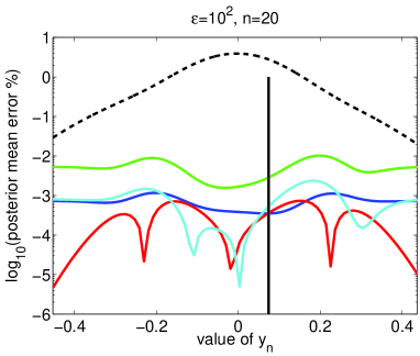
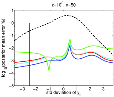
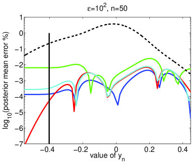
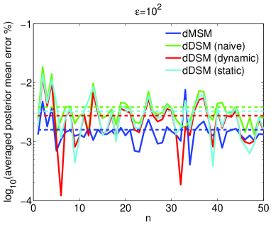
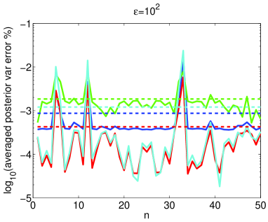
Figure 11: The relative errors of the approximations of the posterior $u_{n}|Y_{n}$ distributions that depend on the realization of $y_{n}=u_{n}+\eta_{n}$, and their statistical averages with respect to the law of $y_{n}$ when $\epsilon=10^{2}$.

Like the preceding case, we take as reference the Gaussian sum filter for SSM with projection of posterior into the set of Gaussian distributions. The overall scenario when $\epsilon=10^{2}$ is similar to the case with $\epsilon=10^{1}$, except that dMSM becomes more accurate. We plot Fig. 10, Fig. 10 and Fig. 11 that correspond to Fig. 7, Fig. 7 and Fig. 8 respectively. We see the overall errors are of the order : dDSM (dynamic calibration) $\simeq$ dMSM $<$ dDSM (static calibration) $<$ dDSM (naive set). Note dMSM is quite accurate in this case because $\epsilon$ is very large.

4.1.5 Summary

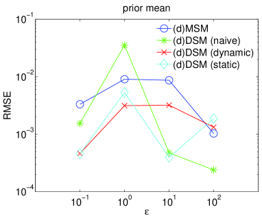
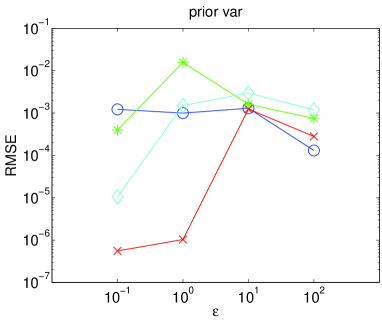
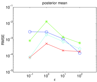
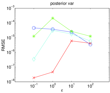
Figure 12: The root mean square errors between the references from SSM filters and the approximations from MSM and DSM filters.

To summarize we plot the root mean square errors of mean and variance between the reference and approximations for all four choices of $\epsilon$ in Fig. 12.

4.2 Supplementary Analysis

This section discusses our choices, especially in relation to choice of reference solution, made while performing numerical simulations in subsection 4.1; it can be skipped without harming the understanding of the main messages of the paper.

4.2.1 Imprecise Scale-Separation Regime

In this case where we take $\epsilon=10^{0}$, to make sure whether either the Gaussian description or the Gaussian sum description is a better approximation of the SSM, what we do is to compare the similarity/distance between MSM (note the derivation corresponds to $\epsilon=0$) and Gaussian approximation of SSM, and that between dMSM (that corresponds to $\epsilon=\infty$) and Gaussian sum approximation of SSM.

To that end, we plot the prior distributions from all four cases, when $n=10$ (and we do the same in the remaining examples), in the left panel of Fig. 15. We see that the dMSM has a one-sided fat tail, which is due to the contribution by the Gaussian kernel evolved while $\gamma$ is in the unstable mode. However this feature is not apparent in the mixture approximation of SSM (in fact both Gaussian and Gaussian mixture approximations of SSM are very similar and unimodal). Furthermore, the $L^{1}$ distance between MSM and SSM (Gaussian) is significantly smaller than the one between dMSM and SSM (Gaussian mixture), as shown in the right panel of Fig. 15. The discussion demonstrates that, in this parameter regime, the Gaussian filter for SSM is more suitable as a reference solution than is the Gaussian sum filter.

4.2.2 Moderately Rare-Event Regime

When $\epsilon=10^{1}$, we plot the four relevant prior distributions in the top-left panel of Fig. 15 . While MSM and SSM (Gaussian) are distant from one another, both dMSM and SSM (Gaussian mixture) are characterized by a one-sided fat tail, in contrast to the case of $\epsilon=10^{0}$, and further are very close to one another. Therefore SSM with the Gaussian sum filter is chosen as the appropriate reference solution.

We turn our attention to the validity of Gaussian approximation of the Gaussian mixture posterior. The top-right panel of Fig. 15 depicts the posterior of SSM (Gaussian mixture), which consists of two kernels. The distribution is well approximated by a single Gaussian that has the same mean and variance. This is due to the sharpness of the likelihood we choose (discussed shortly). We may thus approximate the filtering solution by a Gaussian at every observation time, and we can apply Gaussian sum filters in a computationally tractable way without harming accuracy.

4.2.3 Extremely Rare-Event Regime

With regard to SSM filter, the scenario when $\epsilon=10^{2}$ is the same as the case with $\epsilon=10^{1}$. In the bottom of Fig. 15, the priors of dMSM and SSM (Gaussian sum) are almost indistinguishable, and the SSM posterior is accurately approximated by a Gaussian.

We conclude the current section with further study of the Gaussian approximation of the posterior. Recall we have fixed $R_{n}=0.25E$ thus far. In this case, it is shown that the Gaussian approximation of the posterior can be performed without losing accuracy, but this may not be the case when $R_{n}$ is bigger. In Fig. 15, we plot the prior and posterior with $R_{n}=0.75E$. Due to the flatter likelihood, the posterior with two kernels significantly deviates from the Gaussian approximation. In this case, the Gaussian approximation of the posterior cannot guarantee the accuracy of the filtering solution.

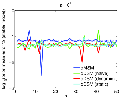
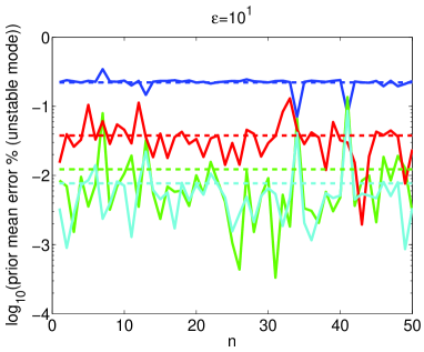
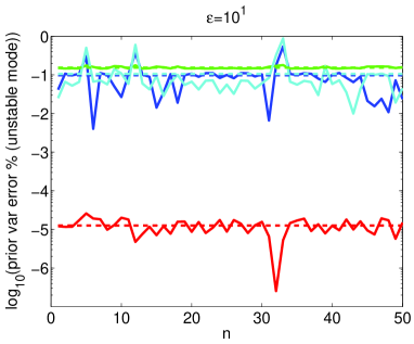
Figure 6: The relative errors of the mean and variance approximations of each Gaussian kernels of the prior distributions when $\epsilon=10^{1}$.

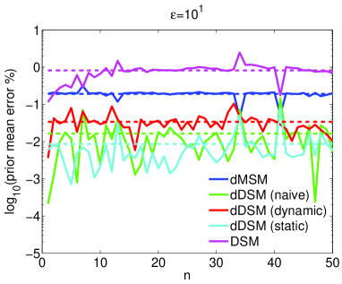
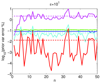
Figure 7: The relative errors of the mean and variance approximations of the prior $u_{n}|Y_{n-1}$ (top) and posterior $u_{n}|Y_{n}$ (bottom) distributions when $\epsilon=10^{1}$.

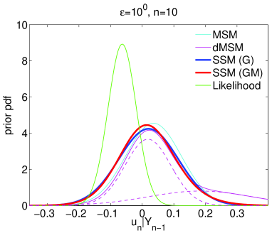
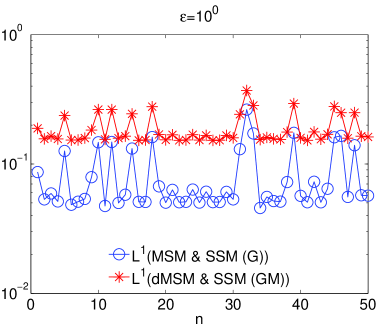
Figure 13: The Gaussian and Gaussian mixture approximations of SSM (labeled SSM(G) and SSM(GM) respectively) together with MSM and dMSM when $\epsilon=10^{0}$. The dashed lines represent two Gaussian kernels consisting of dMSM (left).

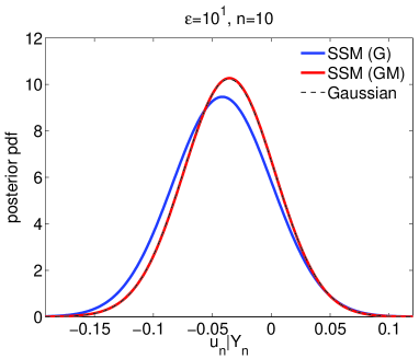
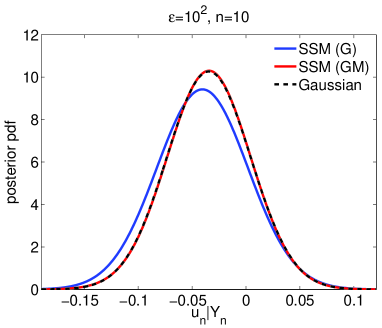
Figure 14: The Gaussian and Gaussian mixture approximations of SSM prior (left) and Gaussian approximations of SSM posterior (right) when $\epsilon=10^{1}$ (top) and $\epsilon=10^{2}$ (bottom). The dashed lines are two Gaussian kernels of SSM approximation (top-left) and Gaussian approximation of Gaussian mixture SSM (right).

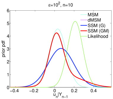
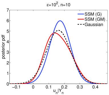
Figure 15: The Gaussian and Gaussian sum approximations of SSM prior (left) and Gaussian approximations of SSM posterior (right) when $\epsilon=10^{2}$ and $R=0.75E$.

5 Conclusions

In this paper we have employed simplified models for the estimation of a partially observed turbulent signal. Our test bed, the switching stochastic model (SSM), is a stochastic differential equation driven by a sign-alternating two-state Markov process. The system is either forced or dissipated depending on the sign of the driving signal, and as a consequence exhibits intermittent turbulent bursting. It is a cheap surrogate for turbulent signal generation, allowing rapid prototyping of a variety of approximate filters – filters with model error. Two approximate models (MSM, DSM) for SSM have been constructed via simplification of the switching process underlying the turbulent bursting, leading to a Gaussian description for the filtering solution. We study the moment generating function (MGF) with respect to the time integral of the switching process to reveal that these two models precisely mimic the SSM behavior when the switching frequency is relatively high. In addition to these two models, based on the same argument, we also build two models (dMSM, dDSM) whose regime of validity is rare switching for the driving signal. We associate these two models with Gaussian sum filters.

We first use the ergodicity of the switching processes to prove MSM (dMSM) is the high (low) switching frequency limit of SSM and DSM (dDSM). Besides verifying the consistency of the proposed approximate models, the convergence results give rise to an analytic determination of DSM (dDSM) parameters when the time-scales of driving input and system output are well separated. We achieve this from the comparison between asymptotics of MGFs in each of two opposing parameter regimes, because their matching implies the lower order moments of the corresponding DSM (dDSM) are very close to those of SSM. The result again gives rise to a determination of DSM (dDSM) parameters when two time-scales are weakly separated. In this case, we numerically find a minimizer of the sum-of-squares error function between the mean and variance of SSM and DSM (dDSM) for which the previous analytic solutions is used as the initial candidate. In our numerical simulations, the filtering results utilizing DSM (dDSM) with the parameters tuned according to our suggestions show significant improvements in accuracy in all the parameter regimes that we examined. Furthermore, when the time-scale separation is weak, the cost of performing the minimizations can be alleviated by averaging the parameters calculated only for a number of observation time steps, while maintaining the accuracy of the filtering solution to a considerable extent.

We have used the tools from three different research areas: limit theorems, asymptotic analysis and computational optimization to complete the whole scenario. These methods are not separate but carefully chained together through a solution cascade to provide a significant step in the analysis and development of filters utilizing approximate models suggested from a rigorous analysis of the underlying system. As the ultimate goal of filtering with model error is to estimate the system state and associated uncertainties of real-world turbulence, at tractable cost, our future work will include the development of these algorithms, and their benchmarking, in the case where the true signal is not generated by SSM, but rather by a real turbulence model.

Appendix A Switching Stochastic Model

Here we analyze SSM. Subsection A.1 is with regard to the computation of MGFs of integral process of driving signal, and subsection A.2 to their asymptotic behaviors. We develop SSM filters in subsection A.3. Note $\epsilon$ in $\lambda_{+}/\epsilon$ and $\lambda_{-}/\epsilon$ is dropped out for the notational economy.

A.1 Moment generating function (MGF) of integral process

Here we aim to analytically compute

$$\begin{split}&\left\langle e^{\alpha(\Gamma_{T}-\Gamma_{t})}\right\rangle\\ &\left\langle e^{\alpha(\Gamma_{T}-\Gamma_{t})}|\gamma_{0}=\gamma_{\pm}\right\rangle\end{split}$$ (A.1)

where $\Gamma_{t}=\int^{t}_{0}{\gamma}(s)ds$.

We first point out that it suffices provide the formula for

$$\begin{split}\left\langle e^{\alpha\Gamma_{t}}|\gamma_{0}=\gamma_{+}\right\rangle.\end{split}$$ (A.2)

Once it is done, that of $\left\langle e^{\alpha\Gamma_{t}}|\gamma_{0}=\gamma_{-}\right\rangle$ is immediate from the exchange $(\lambda_{+},\gamma_{+})\leftrightarrow(\lambda_{-},\gamma_{-})$. Because $\rho_{\gamma}(t)\equiv(\mathbb{P}(\gamma_{t}=\gamma_{+}),\mathbb{P}(\gamma_{t}=\gamma_{-}))^{t}$ solves $d{\rho}_{\gamma}(t)/{dt}=L^{t}\rho_{\gamma}(t)$, where upper $t$ denotes transpose and

$$L\equiv\left(\begin{array}[]{cc}-\lambda_{+}&\lambda_{+}\\ \lambda_{-}&-\lambda_{-}\end{array}\right),$$

it satisfies

$$\begin{split}\left(\begin{array}[]{c}\mathbb{P}(\gamma_{t}=\gamma_{+})\\ \mathbb{P}(\gamma_{t}=\gamma_{-})\end{array}\right)&=\frac{1}{\lambda_{+}+\lambda_{-}}\left(\begin{array}[]{cc}\lambda_{-}+\lambda_{+}e^{-(\lambda_{-}+\lambda_{+})t}&\;\lambda_{-}-\lambda_{-}e^{-(\lambda_{-}+\lambda_{+})t}\\ \lambda_{+}-\lambda_{+}e^{-(\lambda_{-}+\lambda_{+})t}&\;\lambda_{+}+\lambda_{-}e^{-(\lambda_{-}+\lambda_{+})t}\end{array}\right)\left(\begin{array}[]{c}\mathbb{P}(\gamma_{0}=\gamma_{+})\\ \mathbb{P}(\gamma_{0}=\gamma_{-})\end{array}\right).\end{split}$$ (A.3)

Then from substituting (A.3) into

$$\begin{split}\left\langle e^{\alpha(\Gamma_{T}-\Gamma_{t})}\right\rangle&=\mathbb{P}(\gamma_{t}=\gamma_{+})\left\langle e^{\alpha(\Gamma_{T}-\Gamma_{t})}|\gamma_{t}=\gamma_{+}\right\rangle+\mathbb{P}(\gamma_{t}=\gamma_{-})\left\langle e^{\alpha(\Gamma_{T}-\Gamma_{t})}|\gamma_{t}=\gamma_{-}\right\rangle\\ &=\mathbb{P}(\gamma_{0}=\gamma_{+})\left\langle e^{\alpha(\Gamma_{T}-\Gamma_{t})}|\gamma_{0}=\gamma_{+}\right\rangle+\mathbb{P}(\gamma_{0}=\gamma_{-})\left\langle e^{\alpha(\Gamma_{T}-\Gamma_{t})}|\gamma_{0}=\gamma_{-}\right\rangle\end{split}$$ (A.4)

it follows that

$$\begin{split}\left\langle e^{\alpha(\Gamma_{T}-\Gamma_{t})}|\gamma_{0}=\gamma_{+}\right\rangle=\frac{1}{\lambda_{+}+\lambda_{-}}&\Bigg{(}\left(\lambda_{-}+\lambda_{+}e^{-(\lambda_{-}+\lambda_{+})t}\right)\left\langle e^{\alpha(\Gamma_{T}-\Gamma_{t})}|\gamma_{t}=\gamma_{+}\right\rangle\\ &\quad+\left(\lambda_{+}-\lambda_{+}e^{-(\lambda_{-}+\lambda_{+})t}\right)\left\langle e^{\alpha(\Gamma_{T}-\Gamma_{t})}|\gamma_{t}=\gamma_{-}\right\rangle\Bigg{)}.\end{split}$$ (A.5)

Making use of $\left\langle e^{\alpha(\Gamma_{T}-\Gamma_{t})}|\gamma_{t}=\gamma_{+}\right\rangle=\left\langle e^{\alpha\Gamma_{T-t}}|\gamma_{0}=\gamma_{+}\right\rangle$, Eqs. (LABEL:eq:ssmmgfjt20) are expressed in terms of (A.2) through (A.4), (A.5).

We next attempt to compute Eq. (A.2). In what follows, we will show that (A.2) is given by (A.8) for identical $\lambda_{+}=\lambda_{-}$, and that (A.2) can be computed with the help of (A.6), (A.9) for distinct $\lambda_{+}\neq\lambda_{-}$. When $\gamma(0)=\gamma_{+}$, let $\gamma_{k}$ denote the value of $\gamma(s)$ after undergoing $k$ transitions, i.e., $\gamma_{k}=\gamma_{+}$ for even $k$ and $\gamma_{k}=\gamma_{-}$ for odd $k$. Let $\tau_{k}\triangleq\tau^{\gamma_{+}}$ for even $k$ and $\tau_{k}\triangleq\tau^{\gamma_{-}}$ for odd $k$. Let $T_{n}=\sum_{k=0}^{n-1}\tau_{k}$ and let $N_{t}=\max\{n\in\mathbb{N}:T_{n}\leq t\}$ denote the number of transitions of $\gamma(s)$ in the interval $s\in(0,t]$. From $\tau_{k}=T_{k+1}-T_{k}$, we have

$$\Gamma_{t}=\int^{t}_{0}{\gamma}(s)ds=\sum_{k=0}^{N_{t}-1}\gamma_{k}\tau_{k}+\gamma_{N_{t}}(t-T_{N_{t}})=\sum_{k=0}^{N_{t}-1}(\gamma_{k}-\gamma_{N_{t}})\tau_{k}+\gamma_{N_{t}}t.$$

Note $\tau\sim\exp(r)$ then $\mathbb{E}(e^{\alpha\tau})=\int_{0}^{\infty}e^{\alpha t}re^{-rt}dt=(1-{\alpha\over r})^{-1}$ for $\alpha<r$. Since $\{\tau_{k}\}_{k=0}^{n-1}$ are mutually independent and $\tau_{k}$ is distributed by exponential distribution, Eq. (A.2) allows for a formal expansion

$$\begin{split}\left\langle e^{\alpha\Gamma_{t}}|\gamma_{0}=\gamma_{+}\right\rangle&=\sum_{n=0}^{\infty}\mathbb{P}(N_{t}=n|\gamma_{0}=\gamma_{+})\left\langle e^{\alpha\left(\sum_{k=0}^{n-1}(\gamma_{k}-\gamma_{n})\tau_{k}+\gamma_{n}t\right)}|\gamma_{0}=\gamma_{+}\right\rangle\\ &=\sum_{\text{n:even}}\mathbb{P}(N_{t}=n|\gamma_{0}=\gamma_{+})e^{\alpha\gamma_{+}t}\left(1-\frac{\alpha(\gamma_{-}-\gamma_{+})}{\lambda_{-}}\right)^{-\frac{n}{2}}\\ &\quad+\sum_{\text{n:odd}}\mathbb{P}(N_{t}=n|\gamma_{0}=\gamma_{+})e^{\alpha\gamma_{-}t}\left(1-\frac{\alpha(\gamma_{+}-\gamma_{-})}{\lambda_{+}}\right)^{-\frac{n+1}{2}}\end{split}$$ (A.6)

for ${\lambda_{-}\over\gamma_{-}-\gamma_{+}}<\alpha<{\lambda_{+}\over\gamma_{+}-\gamma_{-}}$.

To compute $\mathbb{P}(N_{t}=n|\gamma_{0}=\gamma_{+})$, notice

$$\begin{split}\mathbb{P}(N_{t}=n)&=\mathbb{P}(N_{t}\geq n)-\mathbb{P}(N_{t}\geq n+1)\\ &=\mathbb{P}(T_{n}\leq t)-\mathbb{P}(T_{n+1}\leq t)\end{split}$$

which is, in other words,

$$\begin{split}\begin{cases}\mathbb{P}(N_{t}=0)&=1-\int^{t}_{0}f_{1}(s)ds\\ \mathbb{P}(N_{t}=n)&=\int^{t}_{0}f_{n}(s)ds-\int^{t}_{0}f_{n+1}(s)ds,\quad n\geq 1\end{cases}\end{split}$$ (A.7)

where $f_{n}$ denotes the probability density function of $T_{n}$. Let $f_{+}(t)=\lambda_{+}e^{-\lambda_{+}t}$ and $f_{-}(t)=\lambda_{-}e^{-\lambda_{-}t}$, and let $*$ denote the convolution, then

$$\begin{split}f_{m+n}(t)&=(f_{+})^{*m}*(f_{-})^{*n}(t)\\ &=\frac{\lambda_{+}^{m}\lambda_{-}^{n}}{(m-1)!(n-1)!}\int^{t}_{0}s^{m-1}e^{-\lambda_{+}s}(t-s)^{n-1}e^{-\lambda_{-}(t-s)}ds\\ &=\frac{\lambda_{+}^{m}\lambda_{-}^{n}}{(m-1)!(n-1)!}e^{-\lambda_{-}t}t^{m+n-1}\int^{1}_{0}s^{m-1}(1-s)^{n-1}e^{-(\lambda_{+}-\lambda_{-})ts}ds\\ \end{split}$$

with $|m-n|=1$.

A.1.1 $\lambda_{+}=\lambda_{-}$

In case of $\lambda_{+}=\lambda_{-}$, both are denoted by $\lambda$. Note the beta function is given by

$$\int^{1}_{0}s^{m-1}(1-s)^{n-1}ds=\frac{(m-1)!(n-1)!}{(m+n-1)!}$$

and the use of integration by parts yields

$$\begin{split}\int^{t}_{0}{f}_{n}ds=\int^{t}_{0}\lambda^{n}\frac{s^{n-1}}{(n-1)!}e^{-\lambda s}ds=\frac{\lambda^{n}}{n!}t^{n}e^{-\lambda t}+\int^{t}_{0}f_{n+1}ds.\end{split}$$

Therefore, from (A.7), $N_{t}$ is distributed by Poisson distribution with parameter ${\lambda}t$

$$\mathbb{P}(N_{t}=n)=e^{-{\lambda}t}\frac{({\lambda}t)^{n}}{n!}.$$

In this case, $\mathbb{P}(N_{t}=n|\gamma_{0}=\gamma_{+})=\mathbb{P}(N_{t}=n)$ and Eq. (A.6) is summed into the closed form

$$\begin{split}\left\langle e^{\alpha\Gamma_{t}}|\gamma_{0}=\gamma_{+}\right\rangle&=e^{-\lambda t}\Bigg{(}e^{\alpha\gamma_{+}t}\cosh\left(\lambda t\left(1-\frac{\alpha(\gamma_{-}-\gamma_{+})}{\lambda_{-}}\right)^{-\frac{1}{2}}\right)\\ &\quad+e^{\alpha\gamma_{-}t}\sinh\left(\lambda t\left(1-\frac{\alpha(\gamma_{+}-\gamma_{-})}{\lambda_{+}}\right)^{-\frac{1}{2}}\right)\left(1-\frac{\alpha(\gamma_{+}-\gamma_{-})}{\lambda_{+}}\right)^{-\frac{1}{2}}\Bigg{)}\end{split}$$ (A.8)

when $\lambda$ represents $\lambda_{+}=\lambda_{-}$.

A.1.2 $\lambda_{+}\neq\lambda_{-}$

Consider the case where $\lambda_{+}$ and $\lambda_{-}$ are different. Let $B(m,n;\alpha)\equiv\int^{1}_{0}s^{m-1}(1-s)^{n-1}e^{\alpha s}ds$ then integration by parts yields

$$B(m,n;\alpha)=\frac{1}{\alpha}\left[(m-1)B(m-1,n;\alpha)-(n-1)B(m,n-1;\alpha)\right].$$

Using $B(m-1,n;\alpha)=e^{\alpha}B(n,m-1;-\alpha)$ and

$$\int t^{n}e^{\alpha t}dt=\frac{t^{n}e^{\alpha t}}{\alpha}-\frac{n}{\alpha}\int t^{n-1}e^{\alpha t}dt$$

we recursively obtain $f_{n}$ and the probability distribution of $N_{t}$

$$\begin{split}\begin{cases}\mathbb{P}(N_{t}=0|\gamma_{0}=\gamma_{+})&=e^{-\lambda_{+}t}\\ \mathbb{P}(N_{t}=1|\gamma_{0}=\gamma_{+})&=\frac{\lambda_{+}(e^{-\lambda_{+}t}-e^{-\lambda_{-}t})}{-(\lambda_{+}-\lambda_{-})}\\ \mathbb{P}(N_{t}=2|\gamma_{0}=\gamma_{+})&=\frac{\lambda_{-}\lambda_{+}\exp(-\lambda_{-}t)-\lambda_{-}\lambda_{+}\exp(-\lambda_{+}t)+t\lambda_{-}\lambda_{+}(\lambda_{-}-\lambda_{+})\exp(-\lambda_{+}t)}{(\lambda_{-}-\lambda_{+})^{2}}\\ &\cdots\end{cases}\end{split}$$ (A.9)

from (A.7). One can make use of (A.9) to compute a truncation of (A.6). We conclude the section with the following theorem.

Theorem A.1

The RHS of Eq. (A.6) uniformly converges.

Proof A.1.

Let $f^{+}_{n}(s)=(\lambda_{+})^{n}\frac{s^{n-1}}{(n-1)!}e^{-\lambda_{+}s}$ and $f^{-}_{n}(s)=(\lambda_{-})^{n}\frac{s^{n-1}}{(n-1)!}e^{-\lambda_{-}s}$. The inequalities

$$\left(\frac{\lambda_{+}}{\lambda_{-}}\right)^{m}{f}^{-}_{m+n}(t)\leq f_{m+n}(t)\leq\left(\frac{\lambda_{-}}{\lambda_{+}}\right)^{n}{f}^{+}_{m+n}(t).$$

hold from $1\leq e^{-(\lambda_{+}-\lambda_{-})ts}\leq e^{-(\lambda_{+}-\lambda_{-})t}$ for $s\in[0,1]$. Let $f_{m+1+n}(t)=(f_{+})^{*(m+1)}*(f_{-})^{*n}(t)$ then using

$$\begin{split}\int^{t}_{0}\lambda^{n}\frac{s^{n-1}}{(n-1)!}e^{-\lambda s}ds\leq\int^{t}_{0}\lambda^{n}\frac{s^{n-1}}{(n-1)!}ds=\frac{(\lambda t)^{n}}{n!}\end{split}$$

we obtain

$$\begin{split}\int^{t}_{0}\left(f_{m+n}(s)-f_{m+1+n}(s)\right)ds&\leq\int^{t}_{0}\left(\left(\frac{\lambda_{-}}{\lambda_{+}}\right)^{n}{f}^{+}_{m+n}(s)-\left(\frac{\lambda_{+}}{\lambda_{-}}\right)^{m+1}{f}^{-}_{m+1+n}(s)\right)ds\\ &\leq\left(\frac{\lambda_{-}}{\lambda_{+}}\right)^{n}\frac{(\lambda_{+}t)^{m+n}}{(m+n)!}+\left(\frac{\lambda_{+}}{\lambda_{-}}\right)^{m+1}\frac{(\lambda_{-}t)^{m+1+n}}{(m+1+n)!}.\end{split}$$

Therefore when $n$ is even

$$\mathbb{P}(N_{t}=n|\gamma_{0}=\gamma_{+})\leq\left(\frac{\lambda_{-}}{\lambda_{+}}\right)^{\frac{n}{2}}\frac{(\lambda_{+}t)^{n}}{n!}+\left(\frac{\lambda_{+}}{\lambda_{-}}\right)^{\frac{n}{2}+1}\frac{(\lambda_{-}t)^{n+1}}{(n+1)!}$$

is satisfied and a similar bound holds when $n$ is odd. The application of Weierstrass M-test leads to the uniform convergence in view of Eq. (A.8).

A.2 Asymptotics for MGF of integral process

We here derive asymptotic formulae for MGFs (LABEL:eq:ssmmgfjt20), (A.2) when $\epsilon\ll 1$ (scale-separation regime) and $\epsilon\gg 1$ (rare-event regime).

A.2.1 Scale-separation regime

When $\lambda_{+}$ and $\lambda_{-}$ are distinct, and $\epsilon$ is small, we replace $\lambda$ in Eq. (A.8) by the harmonic mean $\bar{\lambda}\equiv\frac{2\lambda_{+}\lambda_{-}}{\lambda_{+}+\lambda_{-}}$ to derive an approximation. This is because the density function of $T_{n}$ is the convolution of $f_{+}=\lambda_{+}e^{-\lambda_{+}t}$ and $f_{-}=\lambda_{-}e^{-\lambda_{-}t}$, $n/2$ times respectively, and from

$$\begin{split}\left(1-\frac{i\alpha}{\lambda_{-}}\right)^{-\frac{n}{2}}\left(1-\frac{i\alpha}{\lambda_{+}}\right)^{-\frac{n}{2}}\simeq\left(1-\frac{i\alpha}{\bar{\lambda}}\right)^{-{n}}\end{split}$$

we see $T_{n}\sim f_{-}^{*n/2}*f_{+}^{*n/2}\simeq f$ where $f$ is the gamma distribution with rate $\bar{\lambda}$. Note $P(N_{t}=n)\simeq e^{-\bar{\lambda}t}(\bar{\lambda}t)^{n}/n!$ from $P(N_{t}\geq n)=P(T_{n}\leq t)$. Therefore we get

$$\begin{split}\left\langle e^{\alpha\Gamma_{t}}|\gamma_{0}=\gamma_{+}\right\rangle&\simeq e^{-\bar{\lambda}t}\Bigg{(}e^{\alpha\gamma_{+}t}\cosh\left(\bar{\lambda}t\left(1-\frac{\alpha(\gamma_{-}-\gamma_{+})}{\lambda_{-}}\right)^{-\frac{1}{2}}\right)\\ &\quad+e^{\alpha\gamma_{-}t}\sinh\left(\bar{\lambda}t\left(1-\frac{\alpha(\gamma_{+}-\gamma_{-})}{\lambda_{+}}\right)^{-\frac{1}{2}}\right)\left(1-\frac{\alpha(\gamma_{+}-\gamma_{-})}{\lambda_{+}}\right)^{-\frac{1}{2}}\Bigg{)}\\ &\simeq\exp\left(\alpha\bar{\gamma}_{\infty}t+\alpha^{2}\frac{3}{8}\frac{(\gamma_{-}-\gamma_{+})^{2}(\lambda_{-}^{2}+\lambda_{+}^{2})}{\lambda_{-}\lambda_{+}(\lambda_{+}+\lambda_{-})}t+\frac{\alpha(\gamma_{+}-\gamma_{-})}{4\lambda_{+}}\right)\end{split}$$

and the rescaling $\lambda_{\pm}\to{\lambda_{\pm}}/{\epsilon}$ yields

$$\begin{split}\left\langle e^{\alpha\Gamma_{t}}|\gamma_{0}=\gamma_{+}\right\rangle\simeq\exp\left(\alpha\bar{\gamma}_{\infty}t+\alpha^{2}\frac{3}{8}\frac{(\gamma_{-}-\gamma_{+})^{2}(\lambda_{-}^{2}+\lambda_{+}^{2})}{\lambda_{-}\lambda_{+}(\lambda_{+}+\lambda_{-})}t\epsilon+\frac{\alpha(\gamma_{+}-\gamma_{-})}{4\lambda_{+}}\epsilon+\mathcal{O}(\epsilon^{2})\right)\end{split}$$

where $(1+x)^{k}=1+kx+(k(k-1)/2!)x^{2}+\cdots$ and $\frac{1}{2}e^{x+\alpha\epsilon}+\frac{1}{2}e^{x+\beta\epsilon}(1+\gamma\epsilon)\simeq e^{x+((\alpha+\beta+\gamma)/2)\epsilon}$ is used.

Further we use $ce^{A+\alpha\epsilon}+(1-c)e^{A+\beta\epsilon}\simeq e^{A+(c\alpha+(1-c)\beta)\epsilon}$ to obtain

$$\begin{split}\left\langle e^{\alpha(\Gamma_{T}-\Gamma_{t})}\right\rangle&\simeq\exp\Bigg{(}\alpha\bar{\gamma}_{\infty}(T-t)+\alpha^{2}\frac{3}{8}\frac{(\gamma_{-}-\gamma_{+})^{2}(\lambda_{-}^{2}+\lambda_{+}^{2})}{\lambda_{-}\lambda_{+}(\lambda_{+}+\lambda_{-})}(T-t)\epsilon\\ &\qquad+\alpha\left(\mathbb{P}(\gamma_{0}=\gamma_{+})\frac{(\gamma_{+}-\gamma_{-})}{4\lambda_{+}}+\mathbb{P}(\gamma_{0}=\gamma_{-})\frac{(\gamma_{-}-\gamma_{+})}{4\lambda_{-}}\right)\epsilon+\mathcal{O}(\epsilon^{2})\Bigg{)}\end{split}$$

when $\epsilon<T-t$.

A.2.2 Rare-event regime

When $\epsilon$ is large, we leave the first term in Eq. (A.6) to obtain

$$\begin{split}\left\langle e^{\alpha\Gamma_{T}}\right\rangle&=\mathbb{P}(\gamma_{0}=\gamma_{+})\left\langle e^{\alpha\Gamma_{T}}|\gamma_{0}=\gamma_{+}\right\rangle+\mathbb{P}(\gamma_{0}=\gamma_{-})\left\langle e^{\alpha\Gamma_{T}}|\gamma_{0}=\gamma_{-}\right\rangle\\ &\simeq\mathbb{P}(\gamma_{0}=\gamma_{+})\exp\left(-\frac{\lambda_{+}}{\epsilon}t+\alpha\gamma_{+}t\right)+\mathbb{P}(\gamma_{0}=\gamma_{-})\exp\left(-\frac{\lambda_{-}}{\epsilon}t+\alpha\gamma_{-}t\right).\end{split}$$ (A.10)

A.3 Filters for SSM

Here we make use of the calculations given in subsection A.1 to define Gaussian filter and Gaussian sum filter for SSM.

A.3.1 Gaussian filter

We design the filter as the assumed density filter. Accordingly we assume $u_{0}$ to be Gaussian, and further assume the independence of $(u_{0},\gamma_{0})$ hence that of $(u_{0},\Gamma_{T})$. Then, from Eq. (3.11), it satisfies

$$\begin{split}\left\langle u_{T}\right\rangle&=\left\langle e^{-\Gamma_{T}}\right\rangle\langle u_{0}\rangle\\ \text{Var}(u_{T})&=\left\langle e^{-2\Gamma_{T}}\right\rangle\Big{(}\text{Var}(u_{0})+\langle u_{0}\rangle^{2}\Big{)}-\left\langle e^{-\Gamma_{T}}\right\rangle^{2}\langle u_{0}\rangle^{2}\\ &\quad+\sigma_{u}^{2}\int^{T}_{0}\left\langle e^{-2(\Gamma_{T}-\Gamma_{t})}\right\rangle dt\end{split}$$ (A.11)

for SSM. Either using closed form solution in case of identical $\lambda_{\pm}$ or a truncation of the series solution in case of distinct $\lambda_{\pm}$, one can compute

$$\left\langle e^{\alpha(\Gamma_{T}-\Gamma_{t})}\right\rangle$$

where $\alpha=-1,-2$ and $t\in[0,T]$, and Eq. (A.11). Together with using Eq. (A.3) for the prediction of $\gamma_{t}$, the first two moments mapping for $(u_{0},\gamma_{0})\to(u_{T},\gamma_{T})$ has been achieved. To complete the filter, we apply Kalman data assimilation for $u_{T}$ and keep $\gamma_{T}$ unchanged as this is consistent with Bayes’ rule when $(u_{T},\gamma_{T})$ is independent [12].

A.3.2 Gaussian sum filter

Let $u_{0}$ be Gaussian mixture and the independence of $(u_{0},\gamma_{0})$ be assumed. Using

$$\begin{split}\mathbb{P}({u}_{T})=\mathbb{P}({\gamma}_{0}=\gamma_{+})\mathbb{P}({u}_{T}|{\gamma}_{0}=\gamma_{+})+\mathbb{P}({\gamma}_{0}=\gamma_{-})\mathbb{P}({u}_{T}|{\gamma}_{0}=\gamma_{-})\end{split}$$

we approximate $u_{T}$ as Gaussian mixture with doubled Gaussian kernels. Similarly with Eq. (A.11), the mean and variance of $u_{T}|\gamma_{0}=\gamma_{\pm}$ are determined by

$$\left\langle e^{\alpha(\Gamma_{T}-\Gamma_{t})}|\gamma_{0}=\gamma_{\pm}\right\rangle$$

where $\alpha=-1,-2$ and $t\in[0,T]$. Using prior calculations, the conditioned mean and variance of each kernel are obtained. Then, using Eq. (A.3) for the prediction of $\gamma_{t}$, the algorithm of $(u_{0},\gamma_{0})\to(u_{T},\gamma_{T})$ is established.

To complete the filter, we apply Kalman data assimilation for each Gaussian kernel of $u_{T}$ with care of weights, while preserving the law of $\gamma_{T}$. Because the latter procedure preserves the number of Gaussians, total $2^{n}$ weighted Gaussian kernels describe the posterior distribution after $n$ inter-observation time steps provided $u_{0}$ is Gaussian.

Appendix B Diffusive Stochastic Models

This section is concerned with DSM and dDSM. The moments mapping formulae of DSM are derived in subsection B.1. We study the computation of MGFs of integral process in subsection B.2 and their asymptotic behaviors in subsection B.3.

B.1 DSM moments mapping

We in this subsection provide the moments mapping of

$$\begin{split}\begin{cases}du&=-\gamma u\,dt+\sigma_{u}dB_{u}\\ d\gamma&=-d_{\gamma}(\gamma-\bar{\gamma})\,dt+\sigma_{\gamma}dB_{\gamma}\end{cases}\end{split}$$

when $(u_{0},\gamma_{0})$ is Gaussian. Let $\Gamma_{\gamma}(t)\equiv\int^{t}_{0}\gamma(s)ds$ then the path-wise solutions read

$$\begin{split}u_{t}&=e^{-\Gamma_{\gamma}(t)}u_{0}+\sigma_{u}\int^{t}_{0}e^{-(\Gamma_{\gamma}(t)-\Gamma_{\gamma}(s))}dB_{u}(s)\equiv{A}_{t}+{B}_{t}\\ \gamma_{t}&=\bar{\gamma}+(\gamma_{0}-\bar{\gamma})e^{-d_{\gamma}t}+\sigma_{\gamma}\int^{t}_{0}e^{-d_{\gamma}(t-s)}dB_{\gamma}(s).\end{split}$$

Define

$$\begin{split}b_{\gamma}(t)&\equiv(1-e^{-d_{\gamma}t)})/{d_{\gamma}}\\ \mathcal{B}_{\gamma}(t)&\equiv\sigma_{\gamma}\int^{t}_{0}ds\int^{s}_{0}e^{-d_{\gamma}(s-s^{\prime})}dB_{\gamma}(s^{\prime})\end{split}$$

then $\Gamma_{\gamma}(t)=\bar{\gamma}(t-b_{\gamma}(t))+b_{\gamma}(t)\gamma_{0}+\mathcal{B}_{\gamma}(t)$ and we have

$$\begin{split}\langle u_{t}\rangle&=\langle A_{t}\rangle\\ \langle\gamma_{t}\rangle&=\bar{\gamma}+(\langle\gamma_{0}\rangle-\bar{\gamma})e^{-d_{\gamma}t}\\ \text{Var}(u_{t})&=\langle u_{t}^{2}\rangle-\langle u_{t}\rangle^{2}=\langle A_{t}^{2}\rangle+\langle B_{t}^{2}\rangle-\langle A_{t}\rangle^{2}\\ \text{Var}(\gamma_{t})&=e^{-2d_{\gamma}t}\text{Var}(\gamma_{0})+\frac{\sigma_{\gamma}^{2}}{2d_{\gamma}}\left(1-e^{-2d_{\gamma}t}\right)\\ \text{Cov}(u_{t},\gamma_{t})&=\langle u_{t}\gamma_{t}\rangle-\langle u_{t}\rangle\langle\gamma_{t}\rangle=\bar{\gamma}\left(1-e^{-d_{\gamma}t}\right)\langle A_{t}\rangle+e^{-d_{\gamma}t}\langle A_{t}\gamma_{0}\rangle\\ &\qquad\qquad\qquad\qquad\qquad+\langle A_{t}\dot{\mathcal{B}}_{\gamma}(t)\rangle-\langle A_{t}\rangle\langle\gamma_{t}\rangle\\ \end{split}$$ (B.1)

where upper dot denotes derivative.

Using

$$\begin{split}\langle\Gamma_{\gamma}(t)-\Gamma_{\gamma}(s)\rangle&=\left(b_{\gamma}(t)-b_{\gamma}(s)\right)\langle\gamma_{0}\rangle+\bar{\gamma}((t-s)-(b_{\gamma}(t)-b_{\gamma}(s)))\\ \text{Var}\left(\Gamma_{\gamma}(t)-\Gamma_{\gamma}(s)\right)&=\left(b_{\gamma}(t)-b_{\gamma}(s)\right)^{2}\text{Var}(\gamma_{0})+\text{Var}\left(\mathcal{B}_{\gamma}(t)-\mathcal{B}_{\gamma}(s)\right)\\ \langle\mathcal{B}_{\gamma}(t)\rangle&=0\\ \text{Var}(\mathcal{B}_{\gamma}(t))&=-\frac{\sigma_{\gamma}^{2}}{2d_{\gamma}^{3}}\left(3-4e^{-d_{\gamma}t}+e^{-2d_{\gamma}t}-2d_{\gamma}t\right)\\ \text{Var}(\mathcal{B}_{\gamma}(t)-\mathcal{B}_{\gamma}(s))&=-\frac{\sigma_{\gamma}^{2}}{d_{\gamma}^{3}}\left(1+d_{\gamma}(s-t)+e^{-d_{\gamma}(s+t)}\times\left(-1-e^{2d_{\gamma}s}+\cosh(d_{\gamma}(s-t))\right)\right)\\ \left\langle e^{-\mathcal{B}_{\gamma}(t)}\dot{\mathcal{B}}_{\gamma}(t)\right\rangle&=-\frac{1}{2}\partial_{t}\left(\text{Var}(\mathcal{B}_{\gamma}(t))\right)\left\langle e^{-\mathcal{B}_{\gamma}(t)}\right\rangle\end{split}$$

and using

$$\begin{split}\langle e^{z}\rangle&=e^{\langle z\rangle+\frac{1}{2}\text{Var}(z)}\\ \langle e^{z}x\rangle&=e^{\langle z\rangle+\frac{1}{2}\text{Var}(z)}\big{(}\langle x\rangle+\text{Cov}(x,z)\big{)}\\ \langle e^{z}xy\rangle&=e^{\langle z\rangle+\frac{1}{2}\text{Var}(z)}\Big{(}\text{Cov}(x,y)+\big{(}\langle x\rangle+\text{Cov}(x,z)\big{)}\big{(}\langle y\rangle+\text{Cov}(y,z)\big{)}\Big{)}\end{split}$$

where $(x,y,z)$ is joint Gaussian, we can compute

$$\begin{split}\left\langle A_{t}\right\rangle=\left\langle e^{-\Gamma_{\gamma}(t)}u_{0}\right\rangle&=e^{-\bar{\gamma}(t-b_{\gamma}(t))}\left\langle e^{-b_{\gamma}(t)\gamma_{0}}u_{0}\right\rangle\left\langle e^{-\mathcal{B}_{\gamma}(t)}\right\rangle\\ \left\langle A_{t}\gamma_{0}\right\rangle=\left\langle e^{-\Gamma_{T}}u_{0}\gamma_{0}\right\rangle&=e^{-\bar{\gamma}(t-b_{\gamma}(t))}\left\langle e^{-b_{\gamma}(t)\gamma_{0}}u_{0}\gamma_{0}\right\rangle\left\langle e^{-\mathcal{B}_{\gamma}(t)}\right\rangle\\ \left\langle A_{t}\dot{\mathcal{B}}_{\gamma}(t)\right\rangle=\left\langle e^{-\Gamma_{T}}u_{0}\dot{\mathcal{B}}_{\gamma}(t)\right\rangle&=e^{-\bar{\gamma}(t-b_{\gamma}(t))}\left\langle e^{-b_{\gamma}(t)\gamma_{0}}u_{0}\right\rangle\left\langle e^{-\mathcal{B}_{\gamma}(t)}\dot{\mathcal{B}}_{\gamma}(t)\right\rangle\\ \left\langle A_{t}^{2}\right\rangle=\left\langle e^{-2\Gamma_{T}}u_{0}^{2}\right\rangle&=e^{-2\bar{\gamma}(t-b_{\gamma}(t))}\left\langle e^{-2b_{\gamma}(t)\gamma_{0}}u_{0}^{2}\right\rangle\left\langle e^{-2\mathcal{B}_{\gamma}(t)}\right\rangle\\ \langle B_{t}^{2}\rangle&=\sigma_{u}^{2}\int^{t}_{0}\left\langle e^{-2(\Gamma_{\gamma}(t)-\Gamma_{\gamma}(s))}\right\rangle ds\\ &=\sigma_{u}^{2}\int^{t}_{0}e^{-2\langle\Gamma_{\gamma}(t)-\Gamma_{\gamma}(s)\rangle+2\text{Var}\left(\Gamma_{\gamma}(t)-\Gamma_{\gamma}(s)\right)}ds\end{split}$$

and thereby Eq. (B.1). Here numerical integrator like the trapezoidal rule can be employed for the computation of $\langle B_{t}^{2}\rangle$. As a consequence, the analytic moment-mapping $(u_{0},\gamma_{0})\to(u_{t},\gamma_{t})$ is obtained.

B.2 Moment generating function of integral process

Recall

$$\begin{split}\textbf{(DSM)}\qquad\left\{\begin{array}[]{ll}d\widehat{u}&=-\widehat{\gamma}\widehat{u}\,dt+\sigma_{u}dB_{u}\\ d\widehat{\gamma}&=-\frac{\nu}{\epsilon}(\widehat{\gamma}-\mu)\,dt+\frac{\sigma}{\sqrt{\epsilon}}dB_{\gamma}\\ \end{array}\right.\end{split}$$

and $\widehat{\Gamma}_{t}=\int^{t}_{0}\widehat{\gamma}(s)ds$ then, from the preceding subsection, we have

$$\begin{split}\langle\widehat{\Gamma}_{t}\rangle&=\mu t+\left\langle\widehat{\gamma}_{0}-\mu\right\rangle b_{\gamma}(t)\\ \text{Var}(\widehat{\Gamma}_{t})&=\text{Var}(\widehat{\gamma}_{0})b_{\gamma}(t)^{2}+\text{Var}(\mathcal{B}_{\gamma}(t))\\ \langle\widehat{\Gamma}_{t}-\widehat{\Gamma}_{s}\rangle&=b_{\gamma}(t-s)\langle\widehat{\gamma}_{s}\rangle+\mu((t-s)-b_{\gamma}(t-s))\\ \text{Var}(\widehat{\Gamma}_{t}-\widehat{\Gamma}_{s})&=(b_{\gamma}(t-s))^{2}\text{Var}(\widehat{\gamma}_{s})+\text{Var}\left(\mathcal{B}_{\gamma}(t-s)\right)\\ \langle\widehat{\gamma}_{t}\rangle&=\mu+(\langle\widehat{\gamma}_{0}\rangle-\mu)e^{-\nu t/\epsilon}\\ \text{Var}(\widehat{\gamma}_{t})&=e^{-2\nu t/\epsilon}\text{Var}(\widehat{\gamma}_{0})+\frac{\sigma^{2}}{2\nu}\left(1-e^{-2\nu t/\epsilon}\right)\\ \end{split}$$

where

$$\begin{split}b_{\gamma}(t)&=\epsilon(1-e^{-\nu t/\epsilon)})/{\nu}\\ \text{Var}(\mathcal{B}_{\gamma}(t))&=-\epsilon^{2}\frac{\sigma^{2}}{2\nu^{3}}\left(3-4e^{-\nu t/\epsilon}+e^{-2\nu t/\epsilon}-2\nu t/\epsilon\right).\end{split}$$

Let $\widehat{\gamma}_{0}$ be Gaussian then $\widehat{\Gamma}_{t}$ is Gaussian as well, and the MGFs

$$\begin{split}\left\langle e^{\alpha\widehat{\Gamma}_{t}}\right\rangle&=\exp\left({\alpha\langle\widehat{\Gamma}_{t}\rangle+\frac{\alpha^{2}}{2}\text{Var}(\widehat{\Gamma}_{t})}\right)\\ \left\langle e^{\alpha(\widehat{\Gamma}_{t}-\widehat{\Gamma}_{s})}\right\rangle&=\exp\left({\alpha\langle\widehat{\Gamma}_{t}-\widehat{\Gamma}_{s}\rangle+\frac{\alpha^{2}}{2}\text{Var}(\widehat{\Gamma}_{t}-\widehat{\Gamma}_{s})}\right)\end{split}$$ (B.2)

can be computed.

B.3 Asymptotics of MGFs of integral process

B.3.1 Scale-separation regime

For small $\epsilon$, from substituting $b_{\gamma}(t)=\frac{1}{d}\epsilon+\mathcal{O}(\epsilon^{2})$ and $\text{Var}(\mathcal{B}_{\gamma}(t)-\mathcal{B}_{\gamma}(s))=\frac{\sigma^{2}}{d^{2}}(t-s)\epsilon+\mathcal{O}(\epsilon^{2})$ into (B.2), we obtain

$$\begin{split}\left\langle e^{\alpha\widehat{\Gamma}_{t}}\right\rangle&=\exp\left(\alpha\left(\mu t+\langle\widehat{\gamma}_{0}-\mu\rangle\frac{\epsilon}{\nu}\right)+\alpha^{2}\frac{\sigma^{2}}{2\nu^{2}}t\epsilon+\mathcal{O}(\epsilon^{2})\right)\quad\epsilon<t\\ \left\langle e^{\alpha(\widehat{\Gamma}_{t}-\widehat{\Gamma}_{s})}\right\rangle&=\exp\left(\alpha\mu(t-s)+\alpha^{2}\frac{\sigma^{2}}{2\nu^{2}}(t-s)\epsilon+\mathcal{O}(\epsilon^{2})\right)\quad\epsilon<s.\end{split}$$

B.3.2 Rare-event regime

When $\epsilon$ is large, we use $b_{r}(t)=t-\frac{1}{2}\nu t^{2}/\epsilon+\mathcal{O}(1/\epsilon^{2})$ and $\text{Var}(\mathcal{B}_{\gamma}(t))=\frac{\sigma^{2}}{3}t^{3}/\epsilon+\mathcal{O}(1/\epsilon^{2})$ to obtain

$$\begin{split}\left\langle e^{\alpha\widehat{\Gamma}_{t}}\right\rangle&=\exp\Bigg{(}\alpha\left(\mu t+\langle\widehat{\gamma}_{0}-\mu\rangle\left(t-\frac{\nu}{2}\frac{t^{2}}{\epsilon}\right)\right)+\frac{\alpha^{2}}{2}\left(\text{Var}(\widehat{\gamma}_{0})\left(t^{2}-\nu\frac{t^{3}}{\epsilon}\right)+\frac{\sigma^{2}}{3}\frac{t^{3}}{\epsilon}\right)\\ &\qquad\qquad+\mathcal{O}\left(\frac{1}{\epsilon^{2}}\right)\Bigg{)}\end{split}$$

for DSM. Therefore, in case of dDSM, we have

$$\begin{split}\left\langle e^{\alpha\widehat{\Gamma}^{\prime}_{t}}|\widehat{\gamma}_{0}^{\prime}=\gamma_{\pm}\right\rangle&=\exp\left(\alpha\left(\mu_{\pm}t+({\gamma}_{\pm}-\mu_{\pm})\left(t-\frac{\nu_{\pm}}{2}\frac{t^{2}}{\epsilon}\right)\right)+\frac{\alpha^{2}}{2}\frac{(\sigma_{\pm})^{2}}{3}\frac{t^{3}}{\epsilon}+\mathcal{O}\left(\frac{1}{\epsilon^{2}}\right)\right)\\ &=\exp\left(\alpha\left({\gamma}_{\pm}t-\frac{1}{2\epsilon}({\gamma}_{\pm}-\mu_{\pm})\nu_{\pm}t^{2}\right)+\frac{\alpha^{2}}{2}\frac{(\sigma_{\pm})^{2}}{3\epsilon}t^{3}+\mathcal{O}\left(\frac{1}{\epsilon^{2}}\right)\right).\end{split}$$ (B.3)

Appendix C Proofs of Theorems

C.1 Scale-Separation Limit

Proof C.1 (of Lemma 3.1).

The convergence of the mean and variance follows from Eq. (3.11) and the bounded convergence theorem.

To show $L^{2}(\Omega;\mathbb{R})$ convergence, from Eq. (3.10) we obtain

$$\begin{split}u_{T}^{\epsilon}-\bar{u}_{T}&=\left(e^{-\Gamma^{\epsilon}_{T}}u_{0}^{\epsilon}-e^{-\bar{\gamma}T}\bar{u}_{0}\right)+\sigma_{u}\int^{T}_{0}\left(e^{-(\Gamma^{\epsilon}_{T}-\Gamma^{\epsilon}_{t})}-e^{-\bar{\gamma}(T-t)}\right)dB_{u}(t)\\ \end{split}$$

and

$$\begin{split}|u_{T}^{\epsilon}-\bar{u}_{T}|^{2}&\leq 2\left\lvert e^{-\Gamma^{\epsilon}_{T}}u_{0}^{\epsilon}-e^{-\bar{\gamma}T}\bar{u}_{0}\right\rvert^{2}+2\sigma_{u}^{2}\left\lvert\int^{T}_{0}\left(e^{-(\Gamma^{\epsilon}_{T}-\Gamma^{\epsilon}_{t})}-e^{-\bar{\gamma}(T-t)}\right)dB_{u}(t)\right\rvert^{2}.\end{split}$$

Use Itô lemma to obtain

$$\begin{split}\left\langle|u_{T}^{\epsilon}-\bar{u}_{T}|^{2}\right\rangle&\leq 2\left\langle\left\lvert e^{-\Gamma^{\epsilon}_{T}}u_{0}^{\epsilon}-e^{-\bar{\gamma}T}\bar{u}_{0}\right\rvert^{2}\right\rangle+2\sigma_{u}^{2}\int^{T}_{0}\left\langle\left\lvert e^{-(\Gamma^{\epsilon}_{T}-\Gamma^{\epsilon}_{t})}-e^{-\bar{\gamma}(T-t)}\right\rvert^{2}\right\rangle dt.\end{split}$$

Here note the term

$$\begin{split}\left\langle e^{-2(\Gamma^{\epsilon}_{T}-\Gamma^{\epsilon}_{t})}\right\rangle-2\left\langle e^{-(\Gamma^{\epsilon}_{T}-\Gamma^{\epsilon}_{t})}\right\rangle e^{-\bar{\gamma}(T-t)}+e^{-2\bar{\gamma}(T-t)}\end{split}$$ (C.1)

converges to zero as $\epsilon\to 0$. Then the bounded convergence theorem ensures the integration of (C.1) also converges to zero as $\epsilon\to 0$. Therefore the convergence

$$\begin{split}\left\langle|u_{T}^{\epsilon}-\bar{u}_{T}|^{2}\right\rangle\to 0\end{split}$$

as $\epsilon\to 0$ holds for any $\gamma^{\epsilon}$.

Now we state and prove Lemma C.1 and Lemma C.2 which will be used to prove Lemma 3.2 and Lemma 3.3.

Lemma C.1

Let $\mathcal{Y}$ be a Markov chain or a diffusion process associated with generator $\frac{1}{\epsilon}Q_{0}$. We assume $\mathcal{Y}$ is an ergodic process with invariant measure $\rho^{\infty}_{\mathcal{Y}}$ satisfying $\text{Null}({Q}_{0})=\text{span}\{\mathbf{1}\}$, $\text{Null}({Q}_{0}^{*})=\text{span}\{\rho^{\infty}_{\mathcal{Y}}\}$. Let $\mathcal{X}$ satisfy the ODE

$$\begin{split}\frac{d\mathcal{X}}{dt}=f(\mathcal{X},\mathcal{Y})\end{split}$$

and let the generator of the combined process $(\mathcal{X},\mathcal{Y})$ be of the form

$$\begin{split}Q=\frac{1}{\epsilon}Q_{0}+Q_{1}.\end{split}$$

Let $\bar{\mathcal{X}}$ satisfy the ODE

$$\begin{split}\frac{d\bar{\mathcal{X}}}{dt}=\bar{Q}_{1}(\bar{\mathcal{X}})=\int f(\bar{\mathcal{X}},\cdot)d\rho^{\infty}_{\mathcal{Y}}(\cdot)\end{split}$$ (C.2)

then, for any $t>0$, $\mathcal{X}(t)$ converges weakly or in distribution to $\bar{\mathcal{X}}(t)$ as $\epsilon\to 0$ (recall $X_{\epsilon}\rightharpoonup X$ is referred to converges weakly provided $\mathbb{E}(f(X_{\epsilon}))\to\mathbb{E}(f(X))$ for any bounded continuous function $f$).

Proof C.2 (of Lemma C.1).

The first step is to show that the averaged ODE is given by Eq. (C.2). Let be $\Phi$ be a bounded continuous function and let

$$\begin{split}v(x,y,t)&=\mathbb{E}(\Phi(\mathcal{X}_{t},\mathcal{Y}_{t})|\mathcal{X}_{0}=x,\mathcal{Y}_{0}=y).\end{split}$$

Then it satisfies the backward equation

$$\begin{split}\partial_{t}{v}(x,y,t)=Q{v}(x,y,t)=\left(\frac{1}{\epsilon}Q_{0}+Q_{1}\right){v}(x,y,t).\end{split}$$ (C.3)

We seek solution $v=v(x,y,t)$ in the form of the multi-scale expansion

$$\begin{split}v=v_{0}+\epsilon v_{1}+\mathcal{O}(\epsilon^{2}).\end{split}$$

From substituting the expansion and equating coefficients of equal powers of $\epsilon$ to zero, we find

$$\begin{split}\mathcal{O}\left(\frac{1}{\epsilon}\right):&\qquad Q_{0}v_{0}=0\\ \mathcal{O}(1):&\qquad Q_{0}v_{1}=-Q_{1}v_{0}+\frac{dv_{0}}{dt}\end{split}$$ (C.4)

and we see $v_{0}$ is independent of $y$ due to $\text{null}(Q_{0})=\mathbf{1}$. The operator $Q_{0}$ is singular and, for Eq. (C.4) to have a solution, the Fredholm alternative implies the solvability condition

$$-Q_{1}v_{0}+\frac{dv_{0}}{dt}\perp\text{Null}(Q_{0}^{*}).$$

For arbitrary $c(x)$, we find

$$\begin{split}\int\int c(x)\left(\frac{dv_{0}}{dt}-Q_{1}v_{0}\right)\,dxd\rho_{\infty}(y)=\int c(x)\left(\frac{dv_{0}}{dt}-\bar{Q}_{1}v_{0}\right)\,dx=0\end{split}$$

implying that

$$\frac{dv_{0}}{dt}-\bar{Q}_{1}v_{0}=0.$$

The second step is to show the weak convergence. Substituting

$$v=v_{0}+\epsilon v_{1}+r$$

into Eq. (C.3) yields

$$\begin{split}\frac{dr}{dt}&=\left(\frac{1}{\epsilon}Q_{0}+Q_{1}\right)r+\epsilon q\\ q&=Q_{1}v_{1}-\frac{dv_{1}}{dt}\end{split}$$

and

$$\begin{split}r(t)=e^{Qt}r(0)+\epsilon\int^{t}_{0}e^{Q(t-s)}q(s)ds\end{split}$$

from the variation-of-constants. From $v(t)=e^{Qt}v(0)$ we obtain $|e^{Qt}|_{\infty}\leq 1$ because $\Phi$ is bounded. We then have

$$\begin{split}|r(t)|_{\infty}&\leq\epsilon|e^{Qt}|_{\infty}|r(0)|_{\infty}+\epsilon\int^{t}_{0}|e^{Q(t-s)}|_{\infty}|q(s)|_{\infty}ds\\ &\leq\epsilon|v_{1}(0)|_{\infty}+\epsilon\int^{t}_{0}|q(s)|_{\infty}ds\\ &\leq\epsilon\left(|v_{1}(0)|_{\infty}+t\sup_{0\leq s\leq t}|q(s)|_{\infty}\right)\end{split}$$

and obtain

$$\begin{split}|v(t)-v_{0}(t)|_{\infty}\leq C(T)\epsilon\end{split}$$

for $0\leq t\leq T$.

Lemma C.2

Let $F_{X_{\epsilon}}(\cdot)\equiv\mathbb{P}(X_{\epsilon}\leq\cdot)$ and $F_{X}$ be the distribution function of $X_{\epsilon}$ and non-random variable $X$, respectively. If

$$\lim_{b\to\infty}e^{\alpha b}(F_{X_{\epsilon}}(b)-1)\to 0$$ (C.5a)

$$\lim_{a\to-\infty}e^{\alpha a}F_{X_{\epsilon}}(a)\to 0$$ (C.5b)

$$\lim_{a\to-\infty,b\to\infty}\int^{b}_{a}\left(F_{X_{\epsilon}}(x)-F_{X}(x)\right)e^{\alpha x}dx\to 0$$ (C.5c)

as $\epsilon\to 0$ then $\left\langle e^{\alpha X_{\epsilon}}\right\rangle\to e^{\alpha X}$ follows. The convergence rate is given by the lowest one in Eq. (C.5).

Proof C.3 (of Lemma C.2).

Use integration by parts to obtain

$$\begin{split}\left\langle e^{\alpha X_{\epsilon}}\right\rangle&=\lim_{a\to-\infty,b\to\infty}\int^{b}_{a}e^{\alpha x}dF_{X_{\epsilon}}(x)\\ &=\lim_{a\to-\infty,b\to\infty}e^{\alpha x}F_{X_{\epsilon}}(x)|^{b}_{a}-\int^{b}_{a}F_{X_{\epsilon}}(x)\alpha e^{\alpha x}dx\\ &=\lim_{b\to\infty}e^{\alpha b}(F_{X_{\epsilon}}(b)-1)-\lim_{a\to-\infty}e^{\alpha a}F_{X_{\epsilon}}(a)+e^{\alpha X}\\ &\quad-\lim_{a\to-\infty,b\to\infty}\int^{b}_{a}\left(F_{X_{\epsilon}}(x)-F_{X}(x)\right)\alpha e^{\alpha x}dx.\end{split}$$

Proof C.4 (of Lemma 3.2).

For a bounded continuous function $\Phi$, let

$$\begin{split}v(x,y_{i},t)&=\mathbb{E}(\Phi(\Gamma_{t},\gamma_{t})|\Gamma_{0}=x,\gamma_{0}=y_{i})\\ \end{split}$$

where $y_{1}=\gamma_{+}$ and $y_{2}=\gamma_{-}$. It satisfies the backward equation

$$\begin{split}\partial_{t}v(x,y_{i},t)&=\sum_{j}L_{ij}v(x,y_{j},t)+y_{i}\partial_{x}v(x,y_{i},t)\\ \end{split}$$

or

$$\begin{split}\partial_{t}{v}(x,t)&=Q{v}(x,t)\\ Q&=\frac{1}{\epsilon}Q_{0}+Q_{1}=\frac{1}{\epsilon}\left(\begin{array}[]{cc}-\lambda_{+}&\lambda_{+}\\ \lambda_{-}&-\lambda_{-}\end{array}\right)+\left(\begin{array}[]{cc}y_{1}\partial_{x}&0\\ 0&y_{2}\partial_{x}\end{array}\right)\end{split}$$

in vector notation. The generator of $\gamma$ is then given by

$$L=\frac{1}{\epsilon}\left(\begin{array}[]{cc}-\lambda_{+}&\lambda_{+}\\ \lambda_{-}&-\lambda_{-}\end{array}\right)$$

and $\gamma$ is ergodic process [36].

From Eq. (A.3), the time invariant measure of $\gamma$ is

$$\begin{split}\rho_{\gamma}^{\infty}=\frac{1}{\lambda_{-}+\lambda_{+}}\left(\begin{array}[]{c}\lambda_{-}\\ \lambda_{+}\end{array}\right)\end{split}$$

or

$$\begin{split}\rho_{\gamma}^{\infty}&\triangleq\frac{\lambda_{-}}{\lambda_{-}+\lambda_{+}}\delta_{\gamma_{+}}+\frac{\lambda_{+}}{\lambda_{-}+\lambda_{+}}\delta_{\gamma_{-}}\end{split}$$

on $\mathbb{R}$. An averaging of

$$\begin{split}\frac{d{\Gamma}}{dt}={\gamma}\end{split}$$

yields

$$\begin{split}\frac{d\bar{\Gamma}}{dt}=\int\gamma d\rho^{\infty}_{\gamma}=\frac{\lambda_{-}\gamma_{+}+\lambda_{+}\gamma_{-}}{\lambda_{-}+\lambda_{+}}\equiv\gamma_{\infty}.\end{split}$$

Let

$$\begin{split}v_{0}(x,t)&=\mathbb{E}(\phi(\bar{\Gamma}_{t})|\bar{\Gamma}_{0}=x)\end{split}$$

where $\phi(\cdot)=\Phi(\cdot,y)$ then

$$\begin{split}\partial_{t}v_{0}(x,t)={\gamma}_{\infty}\partial_{x}v_{0}(x,t)=\bar{Q}_{1}v_{0}(x,t)\end{split}$$

and Lemma C.1 ensures $v(x,y_{i},t)\to v_{0}(x,t)$ as $\epsilon\to 0$. In this case the weak convergence of $\Gamma_{t}$ to $\gamma_{\infty}t$ implies $\Gamma_{T}-\Gamma_{t}\rightharpoonup{\gamma}_{\infty}(T-t)$ from Slutsky’s theorem stating that if $X_{\epsilon}\rightharpoonup X$ and $Y_{\epsilon}\rightharpoonup Y$ as $\epsilon\to 0$, where $Y$ is non-random, then $X_{\epsilon}+Y_{\epsilon}\rightharpoonup X+Y$ as $\epsilon\to 0$.

Let the distribution function of $\Gamma_{T}-\Gamma_{t}$ be denoted by $F_{\Gamma_{T}-\Gamma_{t}}(x)\equiv\mathbb{P}(\Gamma_{T}-\Gamma_{t}\leq x)$ then

$$\begin{split}F_{\Gamma_{T}-\Gamma_{t}}(x)=\begin{cases}&0\qquad\text{for}\quad x<\gamma_{-}(T-t)\\ &1\qquad\text{for}\quad x\geq\gamma_{+}(T-t)\end{cases}\end{split}$$

Taking $a<\gamma_{-}(T-t)$ and $b>\gamma_{+}(T-t)$, Eqs. (C.5a), (C.5b) are satisfied. Note $\Gamma_{T}-\Gamma_{t}\rightharpoonup{\gamma}_{\infty}(T-t)$ is equivalent to $F_{\Gamma_{T}-\Gamma_{t}}(x)\to F_{{\gamma}_{\infty}(T-t)}(x)$ for every $x$ that is continuity point of $F_{{\gamma}_{\infty}(T-t)}$, given by

$$\begin{split}F_{{\gamma}_{\infty}(T-t)}(x)=\begin{cases}&0\qquad\text{for}\quad x<{\gamma}_{\infty}(T-t)\\ &1\qquad\text{for}\quad x\geq{\gamma}_{\infty}(T-t)\end{cases}\end{split}$$

from Lévy-Cramér continuity theorem. Then Eq. (C.5c) is satisfied from the bounded convergence theorem and Lemma C.2 ensures the MGF convergence. The convergence rate of $\left\langle e^{\alpha(\Gamma_{T}-\Gamma_{t})}\right\rangle\to e^{\alpha\gamma_{\infty}(T-t)}$ is equal to the one in

$$\begin{split}\lim_{\epsilon\to 0}\int^{\gamma_{+}(T-t)}_{\gamma_{-}(T-t)}\left(F_{\Gamma_{T}-\Gamma_{t}}(x)-F_{\gamma_{\infty}(T-t)}(x)\right)e^{\alpha x}dx=0.\end{split}$$

Proof C.5 (of Lemma 3.3).

The generator of the system

$$\begin{split}\left\{\begin{array}[]{ll}d\widehat{\Gamma}&=\widehat{\gamma}dt\\ d\widehat{\gamma}&=-\frac{1}{\epsilon}\nabla U(\widehat{\gamma})dt+\frac{1}{\sqrt{\epsilon}}\beta(\widehat{\gamma})dB_{\gamma}\\ \end{array}\right.\end{split}$$

is given by

$$\begin{split}y\partial_{x}+\frac{1}{\epsilon}\left(-\nabla U(y)\partial_{y}+\frac{1}{2}\beta(y)^{2}\partial_{y}^{2}\right)=Q_{1}+\frac{1}{\epsilon}Q_{0}.\end{split}$$

If $\widehat{\gamma}$ is an ergodic process with invariant measure $\rho_{\widehat{\gamma}}^{\infty}$ then Lemma C.1 ensures $\widehat{\Gamma}(t)\rightharpoonup\overline{\widehat{\Gamma}}(t)$ solving

$$\begin{split}\frac{d\overline{\widehat{\Gamma}}}{dt}=\int\widehat{\gamma}d\rho_{\widehat{\gamma}}^{\infty}.\end{split}$$

In case of DSM, the generator reads

$$\begin{split}y\partial_{x}+\frac{1}{\epsilon}\left(-\nu(y-\mu)\partial_{y}+\frac{\sigma^{2}}{2}\partial_{y}^{2}\right)=Q_{1}+\frac{1}{\epsilon}Q_{0}\end{split}$$

and the invariant measure for $\widehat{\gamma}$ is

$$\begin{split}\rho_{\widehat{\gamma}}^{\infty}&=\mathcal{N}\left(\mu,\frac{\sigma^{2}}{2\nu}\right)\end{split}$$

because it solves $Q_{0}^{*}\rho_{\widehat{\gamma}}^{\infty}=0$. Therefore we obtain $\widehat{\Gamma}_{t}\rightharpoonup\mu t$ and further $\widehat{\Gamma}_{T}-\widehat{\Gamma}_{t}\rightharpoonup\mu(T-t)$ from Slutsky’s theorem.

Since $\widehat{\gamma}$ is Gaussian process, we use Chernoff bound $F_{\mathcal{N}(0,1)}(x)\leq\frac{1}{2}e^{-x^{2}/2}$ to meet Eqs. (C.5a), (C.5b). Note Eq. (C.5c) is satisfied from bounded convergence theorem. As a consequence, MGF convergence follows and the analyis of convergence rate is the same with SSM case.

C.2 Rare-Event Limit

Proof C.6 (of Lemma 3.4).

It follows from

$$\begin{split}\left\langle{u}^{\epsilon}_{t}|\gamma^{\epsilon}_{0}=\gamma_{\pm}\right\rangle&=\left\langle e^{-{\Gamma}^{\epsilon}_{t}}{u}^{\epsilon}_{0}|\gamma^{\epsilon}_{0}=\gamma_{\pm}\right\rangle\\ \text{Var}(u^{\epsilon}_{t}|\gamma^{\epsilon}_{0}=\gamma_{\pm})&=\left\langle\left(e^{-{\Gamma}^{\epsilon}_{t}}u_{0}^{\epsilon}\right)^{2}|\gamma^{\epsilon}_{0}=\gamma_{\pm}\right\rangle-\left\langle e^{-{\Gamma}^{\epsilon}_{t}}u^{\epsilon}_{0}|\gamma^{\epsilon}_{0}=\gamma_{\pm}\right\rangle^{2}\\ &\quad+\sigma_{u}^{2}\int^{t}_{0}\left\langle e^{-2({\Gamma}^{\epsilon}_{t}-{\Gamma}^{\epsilon}_{s})}|\gamma^{\epsilon}_{0}=\gamma_{\pm}\right\rangle ds.\end{split}$$

Proof C.7 (of Lemma 3.5).

We take $\epsilon\to\infty$ in Eq. (A.6) and use Theorem A.1. In view of (A.10), this yields the case of $t=0$. We invoke (A.5) to complete proof.

Proof C.8 (of Lemma 3.6).

We take $\epsilon\to\infty$ to Eq. (B.3) for the case of $t=0$. Direct computation of (B.2) leads to the result.

References

• [1] B. Anderson and J. Moore, Optimal filtering, vol. 11, Prentice-hall Englewood Cliffs, NJ, 1979.
• [2] A. F. Bennett, Inverse Methods in Physical Oceanography, Cambridge University Press, 1992.
• [3] A. Bensoussan, J.-L. Lions, and G. Papanicolaou, Asymptotic analysis for periodic structures, vol. 374, American Mathematical Soc., 2011.
• [4] C. M. Bishop et al., Pattern recognition and machine learning, vol. 4, springer New York, 2006.
• [5] T. Bohr, M. Jensen, G. Paladin, and A. Vulpiani, Dynamical systems approach to turbulence, vol. 8, Cambridge Univ Pr, 2005.
• [6] M. Branicki, B. Gershgorin, and A. Majda, Filtering skill for turbulent signals for a suite of nonlinear and linear extended kalman filters, Journal of Computational Physics, 231 (2012), pp. 1462–1498.
• [7] M. Branicki and A. Majda, Dynamic stochastic superresolution of sparsely observed turbulent systems, Journal of Computational Physics, (2013).
• [8] E. Castronovo, J. Harlim, and A. Majda, Mathematical test criteria for filtering complex systems: Plentiful observations, Journal of Computational Physics, 227 (2008), pp. 3678–3714.
• [9] R. Chen and J. Liu, Mixture kalman filters, Journal of the Royal Statistical Society: Series B (Statistical Methodology), 62 (2000), pp. 493–508.
• [10] D. Cioranescu and P. Donato, Introduction to homogenization, (2000).
• [11] D. Crouse, P. Willett, K. Pattipati, and L. Svensson, A look at gaussian mixture reduction algorithms, in Information Fusion (FUSION), 2011 Proceedings of the 14th International Conference on, July 2011, pp. 1–8.
• [12] A. Doucet, N. De Freitas, and N. Gordon, Sequential Monte Carlo methods in practice, Springer Verlag, 2001.
• [13] G. Evensen, Data assimilation: the ensemble Kalman filter, Springer Verlag, 2009.
• [14] U. Frisch, Turbulence, Turbulence, by Uriel Frisch, pp. 310. ISBN 0521457130. Cambridge, UK: Cambridge University Press, January 1996., 1 (1996).
• [15] A. Gelb, Applied optimal estimation, MIT Press, 1974.
• [16] B. Gershgorin, J. Harlim, and A. Majda, Test models for improving filtering with model errors through stochastic parameter estimation, Journal of Computational Physics, 229 (2010), pp. 1–31.
• [17] B. Gershgorin, J. Harlim, and A. J. Majda, Improving filtering and prediction of spatially extended turbulent systems with model errors through stochastic parameter estimation, Journal of Computational Physics, 229 (2010), pp. 32–57.
• [18] B. Gershgorin and A. Majda, A nonlinear test model for filtering slow-fast systems, Communications in Mathematical Sciences, 6 (2008), pp. 611–649.
• [19] Z. Ghahramani and G. E. Hinton, Variational learning for switching state-space models, Neural computation, 12 (2000), pp. 831–864.
• [20] N. Gordon, D. Salmond, and A. Smith, Novel approach to nonlinear/non-gaussian bayesian state estimation, in Radar and Signal Processing, IEE Proceedings F, vol. 140, IET, 1993, pp. 107–113.
• [21] J. Harlim and A. Majda, Filtering nonlinear dynamical systems with linear stochastic models, Nonlinearity, 21 (2008), p. 1281.
• [22] J. Harlim and A. J. Majda, Test models for filtering with superparameterization, Multiscale Modeling & Simulation, 11 (2013), pp. 282–308.
• [23] A. Jazwinski, Stochastic processes and filtering theory, vol. 64. san diego, california: Mathematics in science and engineering, 1970.
• [24] R. Kalman et al., A new approach to linear filtering and prediction problems, Journal of basic Engineering, 82 (1960), pp. 35–45.
• [25] R. E. Kalman and R. S. Bucy, New results in linear filtering and prediction theory, Journal of Basic Engineering, 83 (1961), pp. 95–108.
• [26] E. Kalnay, Atmospheric Modeling, Data Assimilation, and Predictability, Cambridge University Press, 2003.
• [27] S. R. Keating, A. J. Majda, and K. S. Smith, New methods for estimating poleward eddy heat transport using satellite altimetry, Mon. Wea. Rev, (2011).
• [28] H. Kushner, Approximations to optimal nonlinear filters, Automatic Control, IEEE Transactions on, 12 (1967), pp. 546–556.
• [29] K. Law, A. Stuart, and K. Zygalakis, Data Assimilation: A Mathematical Introduction, Springer, 2015.
• [30] A. J. Majda and J. Harlim, Filtering Complex Turbulent Systems, Cambridge University Press, 2012.
• [31] A. J. Majda, J. Harlim, and B. Gershgorin, Mathematical strategies for filtering turbulent dynamical systems, Discrete and Continuous Dynamical Systems, 27 (2010), pp. 441–486.
• [32] X. Mao and C. Yuan, Stochastic differential equations with Markovian switching, World Scientific, 2006.
• [33] P. S. Maybeck, Stochastic models, estimation, and control, vol. 3, Academic Press, 1982.
• [34] K. P. Murphy, Machine learning: a probabilistic perspective, MIT Press, 2012.
• [35] D. S. Oliver, A. C. Reynolds, and N. Liu, Inverse theory for petroleum reservoir characterization and history matching, Cambridge University Press, 2008.
• [36] G. Pavliotis and A. Stuart, Multiscale methods: averaging and homogenization, vol. 53, Springer, 2008.
• [37] S. Reich and C. Cotter, Probabilistic Forecasting and Bayesian Data Assimilation, Cambridge University Press, 2015.
• [38] T. P. Sapsis and A. J. Majda, A statistically accurate modified quasilinear gaussian closure for uncertainty quantification in turbulent dynamical systems, Physica D: Nonlinear Phenomena, (2013).
• [39] H. W. Sorenson and D. L. Alspach, Recursive bayesian estimation using gaussian sums, Automatica, 7 (1971), pp. 465–479.
• [40] A. Stordal, H. Karlsen, G. Nævdal, H. Skaug, and B. Vallès, Bridging the ensemble kalman filter and particle filters: the adaptive gaussian mixture filter, Computational Geosciences, 15 (2011), pp. 293–305.
• [41] J. Walter and C. Schütte, Conditional averaging for diffusive fast-slow systems: a sketch for derivation, in Analysis, Modeling and Simulation of Multiscale Problems, Springer, 2006, pp. 647–682.
• [42] V. Zakharov, V. L’vov, and G. Falkovich, Kolmogorov spectra of turbulence 1. wave turbulence., Kolmogorov spectra of turbulence 1. Wave turbulence., by Zakharov, VE; L’vov, VS; Falkovich, G.. Springer, Berlin (Germany), 1992, 275 p., ISBN 3-540-54533-6,, 1 (1992).