Marginal dimensions of the Potts model with invisible states

Abstract

We reconsider the mean-field Potts model with $q$ interacting and $r$ non-interacting (invisible) states. The model was recently introduced to explain discrepancies between theoretical predictions and experimental observations of phase transitions in some systems where the $Z_{q}$-symmetry is spontaneously broken. We analyse the marginal dimensions of the model, i.e., the value of $r$ at which the order of the phase transition changes. In the $q=2$ case, we determine that value to be $r_{c}=3.65(5)$; there is a second-order phase transition there when $r<r_{c}$ and a first-order one at $r>r_{c}$. We also analyse the region $1\leq q<2$ and show that the change from second to first order there is manifest through a new mechanism involving two marginal values of $r$. The $q=1$ limit gives bond percolation and some intermediary values also have known physical realisations. Above the lower value $r_{c1}$, the order parameters exhibit discontinuities at temperature $\tilde{t}$ below a critical value $t_{c}$. But, provided $r>r_{c1}$ is small enough, this discontinuity does not appear at the phase transition, which is continuous and takes place at $t_{c}$. The larger value $r_{c2}$ marks the point at which the phase transition at $t_{c}$ changes from second to first order. Thus, for $r_{c1}<r<r_{c2}$, the transition at $t_{c}$ remains second order while the order parameter has a discontinuity at $\tilde{t}$. As $r$ increases further, $\tilde{t}$ increases, bringing the discontinuity closer to $t_{c}$. Finally, when $r$ exceeds $r_{c2}$ $\tilde{t}$ coincides with $t_{c}$ and the phase transition becomes first order. This new mechanism indicates how the discontinuity characteristic of first order phase transitions emerges.

, , ,

1 Introduction

The concept of universality - wherein certain features of a system do not depend on its details - plays a central role in understanding physical properties of various multi-particle systems. Continuous (second-order) phase transitions provide examples of phenomenon which exhibit universality [1, 2]. For short-range interacting systems, global factors, such as the dimension of space or the dimensions and symmetries of order parameters, define universal features of such a phase transition. These features are shared by different systems, independently of the details of the system structure. Such systems then belong to the same universality class. This is usually identified by critical exponents, critical amplitude ratios and scaling functions. Another universal quantity, which is intrinsic to the critical behaviour of complex systems, is the marginal dimension which marks the number of order-parameter components for which the order of the phase transition changes.

Examples of such systems include the $O(m)$-symmetric spin models [3]. The transitions there are of second order provided that the space dimension exceeds a lower-critical value $d>d_{lc}$ (where $d_{lc}=1$ for the Ising case $m=1$ and $d_{lc}=2$ for $m\geq 2$) [4, 5]. However, when the $O(m)$ symmetry is broken by the presence of terms invariant under the cubic group (the so-called anisotropic cubic model, relevant for an account of crystalline anisotropy [6, 7]), it leads to the emergence of a marginal dimension $m_{c}$. For given space dimension $d$, $m_{c}(d)$ separates regions where the phase transitions of a given symmetry are of first or of second order. For example, the $d=3$ cubic crystal with three easy axes should undergo either a first- or second-order phase transition provided $m_{c}$ is less than or greater than 3, respectively. Theoretical estimates are in favour of $m_{c}(d=3)<3$ [8, 9], supporting the first-order scenario in these systems [7]. Another example is the $q$-state Potts model [10]. Since this model has a discrete symmetry group, $Z_{q}$, the lower critical dimension is $d_{lc}=1$. The marginal value $q_{c}(d)$, for $d>d_{lc}$, separates the first- and second-order regimes there too. For $d=2$ the transition is of second order for $q\leq q_{c}=4$ and of first order otherwise. For $d=3$, the marginal value $q_{c}$ is below $3$ [11]. More examples of marginal dimensions that separate regions of phase transitions of different types are given by systems with non-collinear ordering [12], frustrations [13], structural disorder [14, 9], and competing fluctuating fields [15].

In this paper we will be interested in marginal dimensions of the Potts model with invisible states [16]. The model has been recently introduced in order to explain discrepancies between theoretical predictions and experimental observations of the phase transition in some two-dimensional systems where the $Z_{3}$-symmetry is spontaneously broken [17]. Although, these systems undergo a ferromagnetic phase transition, it appears to be of first order, whereas a standard Potts model predicts the second order scenario at $d=2$, $q=3$. The model continues to attract considerable interest [21, 18, 22, 19, 25, 23, 24, 20], although, as we will show below, some principal questions about its behaviour remain unsolved. In particular, to explain changes in the marginal number of states (marginal dimension) $q_{c}$ that separates the first and second order regimes, the model introduces $r$ additional Potts states (so-called invisible states) that do not contribute to system’s interaction energy but do contribute to the entropy. Hence, for fixed space dimension $d$ and number of states $q$, the value of $r_{c}$ represents a border separating the first- and second-order regimes.

The question of the marginal dimensionality of the Potts model with invisible states is one of the central issues discussed within the context of this model. The mean-field analysis in the framework of the Bragg-Williams approximation of Refs. [16, 18, 19] lead to an estimate $3<r_{c}<4$ for $q=2$. Obtained, as it is, within the mean-field approach, this estimate does not carry a dependence on the space dimensionality. A different mean-field approach employing 3-regular random (thin) graphs also demonstrates a change in the order of the phase transition, but the value of $r_{c}\simeq 17$ obtained at $q=2$ [20] is much higher than in the Bragg-Williams case. Numerical simulations of the Potts model with invisible states in $d=2$ dimensions gave solid evidence that the model exhibits a first-order phase transition at $q=2,3,4$ for high values of $r$ but it still remains a challenge for numerics to get a more precise estimate of $r_{c}$ [16]. Rigorous results prove the existence of a first-order regime for any $q>0$, provided that $r$ is large enough [23, 24]. Exact results for the value of $r_{c}$ for the model are known for a Bethe lattice [25] too.

In this paper we use the mean-field approach to determine more precise estimates for $r_{c}$ when $q=2$ and to find $r_{c}(q)$ in the region $1\leq q<2$. The aim is to deliver a better understanding of how $r_{c}$ changes with $q$. The region also includes the physically accessible case of bond percolation $q=1$ which is of special interest in its own right.

The rest of this paper is organized as follows. In Section 2 we obtain the expression for the free energy of the Potts model with invisible states in the mean-field approximation. The analysis of marginal dimensions is presented in Section 3. In the concluding section, we summarize the results obtained.

2 Free energy in the mean-field approximation

The Hamiltonian of the $(q+r)$-state Potts model with $r$ invisible states reads [16]

$${\cal H}=-\sum_{<i,j>}\delta_{S_{i},S_{j}}\sum_{\alpha=1}^{q}\delta_{S_{i},\alpha}\delta_{S_{j},\alpha}-h\,\sum_{i}\delta_{S_{i},1},$$ (1)

where, $S_{i}=1,\dots,q,(q+1),\dots,(q+r)$ is a Potts spin variable on a site $i=1,\dots,N$, $\delta_{a,b}$ are Kronecker deltas and $h$ is a magnetic field acting on the first visible state. The first sum in the first term spans all distinct nearest neighbour pairs. Only states with $S_{i}=1,\dots,q$ contribute to the interaction term in the Hamiltonian and without loss of generality we may put the coupling constant there equal to 1. The remaining $r$ states do not contribute to the interaction energy but they increase the number of configurations available, and hence they contribute to the entropy (as well as the internal energy). An external field $h$ is chosen to favour the $S_{i}=1$ state.

As mentioned above, a Bragg-Williams type mean-field calculation and Monte-Carlo simulations in two dimensions lead to the conclusion that with increasing $r$ the phase transition in the model (1) becomes ‘harder’; the second-order transition changes to a first-order one. As $r$ is further increased, the latent heat and the jump in the order parameter also increase at the first-order phase-transition point [16, 18, 19]. Since in the mean-field approximation the transition of the usual $q$-state Potts model is of first order for $q>2$, mean-field analysis of Refs. [16, 18, 19] concentrated on the Ising case $q=2$ to demonstrate the change in the order of the phase transition with increasing of $r$. It was shown that the transition becomes first order for $r>3$. However the value of $r_{c}$ has not yet been determined precisely for $q=2$. Here, we will apply another variant of the mean-field approach to obtain precise estimates for the value of the marginal dimension $r_{c}$ for $q=2$ as well as to analyse the entire $1\leq q\leq 2$ region. Besides the Ising case, this region includes another frequently investigated physically relevant case, namely that of bond percolation, $q=1$ [11]. Another challenge is to observe the continuous change of the marginal dimension $r_{c}(q)$, both because analytic continuation in the number of states is an inherent feature of the field-theoretical description of critical phenomena and because the Potts model at non-integer $q$ is relevant for the description of a number of interesting physical phenomena. To give just a few examples, besides the bond percolation previously mentioned, the limit $q\rightarrow 1$ describes turbulence [27, 28]. Universal spanning trees (Fortuin-Kasteleyn graphs) are described by a zero-state $q=0$ Potts model [29, 30]. This limit is related to an arboreal gas model [31] and resistor networks [32, 33]. The Potts model at $q=1/2$ corresponds to a spin glass model [34, 35], which can be also used to analyze the evolution of syntax and language [36]. Finally, the Potts model in the region $0\leq q<1$ describes gelation and vulcanization processes in branched polymers [37].

To proceed with the mean-field analysis, let us introduce thermodynamic averages

$$\langle\delta_{S_{i},\alpha}\rangle=\left\{\begin{array}[]{ccl}&\mu\,,&\alpha=1,\\ &\nu_{1}\,,&\alpha=2,\dots,q,\\ &\nu_{2}\,,&\alpha=q+1,\dots,r\,.\end{array}\right.$$ (5)

Here, the averaging is performed with respect to the Hamiltonian (1)

$$\langle\dots\rangle=\frac{1}{\cal Z}{\rm Tr}\,(\dots)e^{-\beta{\cal H}},\quad\quad{\mbox{with}}\quad\quad{\cal Z}={\rm Tr}\,e^{-\beta{\cal H}},$$ (6)

in the thermodynamic limit, where $\beta$ is the inverse temperature and the trace is taken over all possible spin configurations.

By (5), in the spirit of the mean-field approximation, we assume that the mean value of a spin in a given state does not depend on its coordinate. Note, that three different averages $\mu$, $\nu_{1}$, and $\nu_{2}$ are necessary to take into account the state favoured by the magnetic field and to discriminate between visible and invisible states. Their high- and low- temperature asymptotics are given in Table 1. At high temperatures all states are equally probable, whereas at low temperatures the direction of symmetry breaking is determined by the direction of the magnetic field.

Table 1: Low and high temperature asymptotics of the thermodynamic averages, Eq. (5), and for the order parameters, Eq. (6).

$\beta\rightarrow\infty$	$\mu=1$	$\nu_{1}=0$	$\nu_{2}=0$	$m_{1}=1$	$m_{2}=1$
$\beta\rightarrow 0$	$\mu=\frac{1}{q+r}$	$\nu_{1}=\frac{1}{q+r}$	$\nu_{2}=\frac{1}{q+r}$	$m_{1}=0$	$m_{2}=0$

This asymptotic behaviour together with an obvious normalization condition:

$$\mu+(q-1)\nu_{1}+r\nu_{2}=1$$ (7)

allows one to define the order parameters:

$$m_{1} = \mu-\nu_{1},$$

$$m_{2} = \mu-\nu_{2}.$$ (8)

Both $m_{1}$ and $m_{2}$ exhibit standard temperature asymtotics in that they vanish for $\beta\rightarrow 0$ and are equal to one for $\beta\rightarrow\infty$, see Table 1. However, as we will see below, only $m_{1}$ has a physical interpretation as a quantity that appears below the transition point and breaks the system symmetry. It is easy to show that also the following conditions are satisfied:

$$\mu = \frac{m_{2}r+m_{1}q+1-m_{1}}{q+r},$$

$$\nu_{1} = \frac{(m_{2}-m_{1})r+1-m_{1}}{q+r},$$

$$\nu_{2} = \frac{(m_{1}-m_{2})q+1-m_{1}}{q+r}.$$ (9)

The first Kronecker $\delta$ in the Hamiltonian (1) is rendered redundant by the other two, so that

$${\cal H}=-\sum_{<i,j>}\sum_{\alpha=1}^{q}\delta_{S_{i},\alpha}\delta_{\alpha,S_{j}}-h\sum_{i}\delta_{S_{i},1}.$$ (10)

To obtain the mean-field Hamiltonian, we represent each Kronecker-delta term as a sum of its mean value and deviation from that mean. Neglecting terms comprising a product of two such deviations,

$${{\cal H}=-\frac{z}{2}\sum_{i}[\mu(2\delta_{1,S_{i}}-\mu)+\sum_{\alpha=2}^{q}(2\delta_{\alpha,S_{i}}-\nu_{1})\nu_{1}]-h\sum_{i}\delta_{S_{i},1},}$$ (11)

where $z$ is the number of the nearest neighbours. For the partition function (6) we then get

$${\cal Z}\,=\,e^{-N\beta{z}(\mu^{2}+(q-1)\nu_{1}^{2})/2}\prod_{i}[e^{\beta(h+z\mu)}+(q-1)e^{\beta z\nu_{1}}+r].$$

We consequently derive the free energy per site as

$$f(m_{1},m_{2}) = -\frac{1}{\beta N}\log{\cal Z}=\frac{z}{2}\Bigg{(}\frac{(m_{1}q-m_{1}+m_{2}r+1)^{2}}{(q+r)^{2}}+$$ (12)

$$\frac{(q-1)(-m_{1}r-m_{1}+m_{2}r+1)^{2}}{(q+r)^{2}}\Bigg{)}-$$

$$\frac{1}{\beta}\log\Bigg{\{}(\exp\Bigg{[}{\beta\left(h+\frac{z(m_{1}q-m_{1}+m_{2}r+1)}{q+r}\right)}\Bigg{]}+$$

$$(q-1)\exp\Bigg{[}{\frac{\beta z(-m_{1}r-m_{1}+m_{2}r+1)}{q+r}}\Bigg{]}+r\Bigg{\}}.$$

For $r=0$ one recovers the free energy of the standard Potts model as a function of a single order parameter $m_{1}$ in the mean-field approximation [26]. Of course, $m_{2}$ does not arise in the standard Potts model. There the transition is of the second order only if $q\leq 2$. In the following, we are interested how the presence of invisible states changes the order of this transition.

3 Phase transition and marginal dimensions

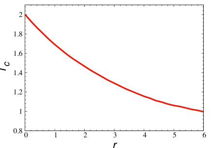
Figure 1: Critical temperature of the Potts model for $q=2$, $z=4$ as a function of the number of invisible states $r$. The critical temperature is a smooth function of $r$ and tends to zero as $r\to\infty$.

With the expression (12) to hand, the thermodynamics of the model are obtained via minimization of the free energy with respect to the two parameters $m_{1}$ and $m_{2}$. In particular, the system of equations that determines the free energy extrema, ${\displaystyle{\partial f/\partial m_{1}=\partial f/\partial m_{2}=0}}$, reads

$$\!\!\!\!\!\!\!\!\!\!\!\!\!\!\frac{(q+r)\left[{e^{\beta(h+m_{1}z)}-r-1}\right]}{e^{\beta(h+m_{1}z)}+re^{\frac{\beta z(m_{1}r+m_{1}-m_{2}r-1)}{q+r}}+q-1} = m_{1}[q+r(r+2)]-r(m_{2}r+1)\,,\quad\quad$$ (13)

$$\!\!\!\!\!\!\!\!\!\!\!\!\!\!\frac{(q+r)\left[{e^{\beta(h+m_{1}z)}+q-1}\right]}{e^{\beta(h+m_{1}z)}+re^{\frac{\beta z(m_{1}r+m_{1}-m_{2}r-1)}{q+r}}+q-1} = -m_{1}r(q-1)+m_{2}qr+q\,.$$ (14)

The solutions of these equations, $m_{1}(T,h)$, $m_{2}(T,h)$ are further analysed to ensure they meet the condition of stability, i.e that they correspond to the free energy minimum, or to local minima in the case of a first-order transition. From these considerations, and numerically solving the system of non-linear equations (13), (14), we find two types of solutions at zero external magnetic field and finite temperature, namely (i) $m_{1}(T,0)=0,\,m_{2}(T,0)\neq 0$ and (ii) $m_{1}(T,0)\neq 0,\,m_{2}(T,0)\neq 0$. Note that $m_{2}(T,0)$ never vanishes at finite temperature. Therefore only $m_{1}(T,0)$ is a proper order parameter, delivering a spontaneous magnetization that signals the occurrence of a phase transition. For fixed $q$, the transition from solution (i) to (ii) occurs at a finite $r$-dependent temperature $T_{c}(r)$.

3.1 The case $q=2$

First let us consider the extension of the Ising model with invisible states. In Fig. 1 we plot the transition temperature for $q=2$ as a function of $r$ for $z=4$. The critical temperature is a smooth function of $r$ and tends to zero as $r\to\infty$. In this limit the system becomes one of non-interacting particles. Note that for the $2D$ Potts model with invisible states on a square lattice $T_{c}$ vanishes for large $(q+r)$ as $T_{c}\approx 2/\ln(q+r)$[23].

      

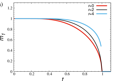
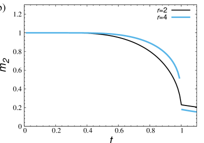
Figure 2: The dependency of the order parameters $m_{1}$ [Panel (a)] and $m_{2}$ [Panel (b)] on the reduced temperature $t=T/T_{c}$ for $r=0,2,4.$ For $r=0$, we only have a single order parameter, namely $m_{1}$. Indeed, $m_{1}(t)$ is a proper order parameter in that it vanishes on one side of the phase transition. In contrast, $m_{2}(t)$ never vanishes at finite temperature. However both $m_{1}$ and $m_{2}$ can be used to distinguish between the first and the second-order regimes as the plots demonstrate.

As has been shown in [16], $r=4$ invisible states are sufficient to change the phase transition of the $q=2$ Potts model from second to first order. This sets an upper bound for the marginal dimension as $r_{c}(q=2)<4$. We display the temperature dependence of the order parameters in Fig. 2 for $r=0,2,4$. Since $T_{c}$ is $r-$dependent we use the reduced temperature $t=T/T_{c}$. As we have noted before, one only has $m_{1}(T)$ for $r=0$. Depending on the value of $r$, the temperature dependency of both order parameters $m_{1}$, $m_{2}$ is characterized by two different regimes. For $r=0,2$ the plots are continuous, signalling second-order phase transitions. However when $r=4$ we observe a jump at the critical temperature. Note that both $m_{1}$ and $m_{2}$ may be used to distinguish between the first and the second order regimes. However, it is worth re-emphasising that above the critical temperature $m_{1}(t)=0$, while $m_{2}(t)$ vanishes only for the infinite temperature.

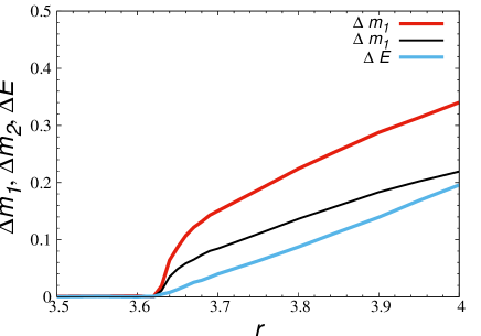
Figure 3: Jumps in the order parameters $\Delta m_{1}$ (red curve), $\Delta m_{2}$ (black curve) and the latent heat $\Delta E$ (blue curve) of the Potts model at $q=2$ as functions of the number of invisible states $r$.

To locate the marginal value $r_{c}$, we define the jump in the order parameters by

$$\Delta m_{j}=\lim_{t\to 1^{-}}m_{j}(t)-\lim_{t\to 1^{+}}m_{j}(t),\hskip 20.00003ptj=1,2,$$ (15)

and analyse the behaviour of $\Delta m_{j}$ as function of $r$. The first appearance of a non-zero value of $\Delta m_{j}$ corresponds to the onset of the first-order phase transition. In Fig. 3 we plot $\Delta m_{1}$ and $\Delta m_{2}$ as functions of the number of invisible states $r$. Similar behaviour is observed for the latent heat $\Delta E=-\Delta S\,T_{c}$, where $\Delta S$ is the entropy jump at the phase transition point:

$$\Delta S=\lim_{t\to 1^{-}}S(t)-\lim_{t\to 1^{+}}S(t).$$ (16)

This is also plotted in Fig. 3. The values of $r_{c}$ obtained from the vanishing of $\Delta m_{1}$, $\Delta m_{2}$, and $\Delta E$ are: $r_{c}=3.629(1)$, $r_{c}=3.627(2)$, and $r_{c}=3.617(3)$, respectively. Averaging these values we get $r_{c}=3.622(8)$. This estimate agrees well with the $z\to\infty$ limit of the result obtained for the Potts model with $q=2$ visible and $r$ invisible states on the Bethe lattice with $z$ nearest neighbours [25]: $r_{c}=\lim_{z\to\infty}\frac{4z}{3(z-1)}\Big{(}\frac{z-1}{z-2}\Big{)}^{2}\simeq 3.62$.

In the vicinity of $r_{c}$, the order parameter jumps can be approximated by a power-law decay:

$$\Delta m_{1}\sim(r-r_{c})^{a_{1}},\hskip 28.45274pt\Delta m_{2}\sim(r-r_{c})^{a_{2}}.$$ (17)

Numerical fits in the interval $r=3.625$ to $4.0$ yield estimates for the exponents: $a_{1}=0.477(10)$ and $a_{2}=0.566(15)$.

3.2 The case $1\leq q<2$

Let us consider now the region $1\leq q<2$. Typical behaviour of the order parameters $m_{1}(t)$ and $m_{2}(t)$ for fixed values of $q$ is shown in Fig. 4. There we plot these functions for $q=1.2$ and $r=4,5,6,7,8,9$. For small values of $r$, $m_{1}(t)$ and $m_{2}(t)$ are smooth functions of $t$ and the transition is second order. We observe that $m_{1}(t)$ vanishes linearly as $t$ approaches $t_{c}=1$ from below. This corresponds to the familiar mean-field result for the percolation critical exponent $\beta=1$.

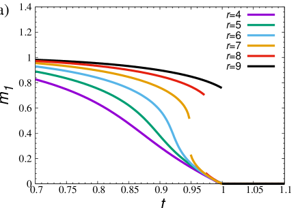
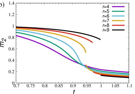
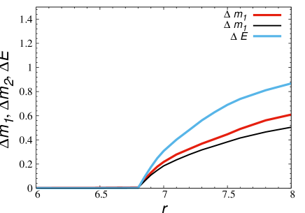
Figure 4: Dependencies of the first (a) and second (b) order parameters on the reduced temperature $t$ for $r=4,5,6,7,8,9$ at $q=1.2$. The second-order phase transition transforms to a first order phase transition at $r_{c_{2}}\simeq 8.495(5)$. Panel (c): discontinuities in the order parameter $\Delta m_{1}$ (red curve), $\Delta m_{2}$ (black curve) and the latent heat $\Delta E$ (blue curve) as functions of $r$ for $q=1.2$ at $t=\tilde{t}$.

For larger values of $r$, and starting from a certain value $r=r_{c1}$, gaps in $m_{1}(t)$ and $m_{2}(t)$ appear at $\tilde{t}<t_{c}$. The marginal dimension $r_{c1}$ obtained from the vanishing of these functions is $r_{c1}\simeq 6.834(11)$. The occurrence of this gap does not affect the order of the phase transition occurring at $t_{c}=1$, which, for these values of $r$, remains second order because the order parameters remain continuous there. The gap at $\tilde{t}$ increases with further increases of $r$ and finally, at $r=r_{c_{2}}$, $\tilde{t}$ and $t_{c}$ coincide. It is at this point that the transition at $t_{c}=1$ becomes first order. The value $r_{c_{2}}$ is therefore the marginal dimension (i.e., it is the value of $r$ at which the phase transition changes its order). It is defined by the condition

$$\Delta m_{1}>0\hskip 10.00002pt{\rm at}\hskip 10.00002ptm_{1}(t\to t_{c}^{+})=0\,.$$ (18)

The occurrence of a gap in the order parameter at temperature $\tilde{t}<t_{c}$ is, to our knowledge, a new phenomenon in the theory of phase transitions.

For $r_{c1}<r<r_{c2}$, the order parameter $m_{1}\neq 0$ in the temperature interval $\tilde{t}<t<t_{c}$. There is no new spontaneous symmetry breaking with respect to $m_{1}$ at $t=\tilde{t}$. However, its jump at $t=\tilde{t}$ is similar to that which occurs in the usual first-order phase transition scenario. Similar behaviour is observed at $t=\tilde{t}$ for the latent heat $\Delta E$ and for $\Delta m_{2}$. These functions are shown in Figs. 4c too.

         

         

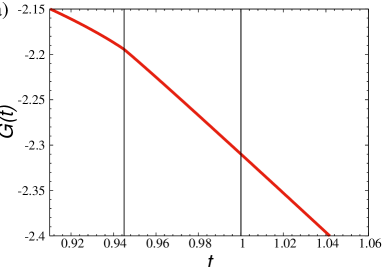
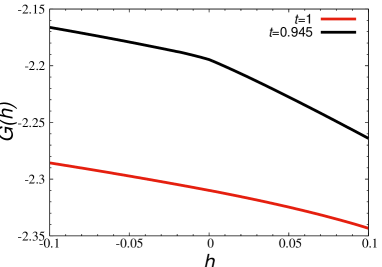
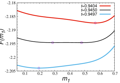
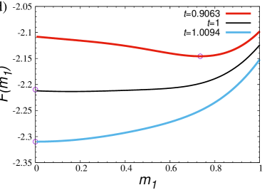
Figure 5: Typical behaviour of the free energy of the Potts model with invisible states at $1\leq q<2$ and $r_{c1}<r<r_{c2}$ ($q=1.2$ and $r=6.96$ for this figure); (a): Gibbs free energy $G(t)$ at $h=0$. Temperatures $\tilde{t}$ and $t_{c}$ are shown by vertical lines. One sees a cusp at $\tilde{t}$, it signals about the presence of a latent heat (a jump in the entropy at $\tilde{t}$); (b): Gibbs free energy $G(h)$ at $t=\tilde{t}$ (upper curve) and at $t=t_{c}$ (lower curve). A cusp in the upper curve signals about a jump in the order parameter at $\tilde{t}$. Note that the cusp is absent in lower curve: the order parameter is continuous at $t_{c}$; (c): Mean-field free energy $F(m_{1})$ at $h=0$ and $t<\tilde{t}$, $t\simeq\tilde{t}=0.945$, $t>\tilde{t}$ (upper, middle, and lower curves, correspondingly); (d): Landau free energy $F(m_{1})$ at $h=0$ and $t<t_{c}$, $t=t_{c}=1$, $t>t_{c}$. The circles in Figs. (c) and (d) show global minima of the free energy.

The behaviour of the Gibbs free energy $G(t,h)$ of the Potts model with invisible states in the region $1\leq q<2$ and $r_{c1}<r<r_{c2}$ is elucidated in Figs. 5 a, b. To this end, we used conditions (13), (14) to eliminate the order-parameter dependency of the mean-field free energy (12) in favour of the external field. In Fig. 5a we display the zero-field Gibbs free energy $G(t,h=0)$ as a function of the reduced temperature $t$. The cusp at $t=\tilde{t}$ signals the jump in the entropy. Fig. 5b shows the Gibbs free energy $G(h)$ at $t=\tilde{t}$ (upper curve) and at $t=t_{c}$ (lower curve). Again, a cusp in the upper curve signals a jump in the order parameter at $\tilde{t}$. However, the cusp is absent in the lower curve: the order parameter is continuous at $t_{c}$. The mean-field free energy $F(m_{1},m_{2})$ is further analysed in Figs. 5c, d. There we show the typical behaviour of the free energy as a function of the first-order parameter $m_{1}$ at $h=0$ in the region of temperatures in the vicinity of $t=\tilde{t}$ (c) and $t=t_{c}$ (d). To get two-dimensional plots, parameter $m_{2}$ has been excluded from the minimum conditions (13), (14). Fig. (c) demonstrates behaviour typical for the first-order phase transition: two minima exist at $t=\tilde{t}=0.945$, see the middle curve of the figure. Different situation is observed in Fig. (d). There, the only value $m_{1}=0$ corresponds to the free energy minimum at $t=t_{c}=1$.

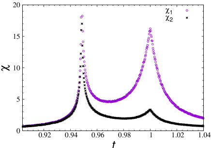
Figure 6: Typical behaviour of the isothermal susceptibilities $\chi_{1}$ and $\chi_{2}$ as functions of reduced temperature for $1<q<2$, $r_{c1}<r<r_{c2}$ ($q=1.2$ and $r=6.96$ in this figure). Distinct peaks are observed at $\tilde{t}$ and $t_{c}$.

To better understand temperature behaviour of the order parameters in the vicinity of $\tilde{t}$, we present, in Fig. 6 typical plots of the isothermal susceptibilities ${\displaystyle{\chi_{1}={{{\partial m_{1}}/{\partial h}}}}}$ and ${\displaystyle{\chi_{2}={{\partial m_{2}}/{\partial h}}}}$ for $1<q<2$ and $r_{c1}<r<r_{c2}$ (specifically, $q=1.2$ and $r=6.96$ in this figure). One observes two distinct peaks located at $\tilde{t}$ and $t_{c}$. The values of the susceptibilities were obtained by numerical evaluation of derivatives in the limit $h\to 0$.

Table 2: Marginal dimensions $r_{c1}$, $r_{c2}$ for different values of $1\leq q\leq 2$.

$q$	$r_{c1}$	$r_{c2}$
1	7.334(49)	9.55(35)
1.1	7.132(7)	8.995(5)
1.2	6.834(11)	8.495(5)
1.3	6.577(5)	8.025(5)
1.4	6.268(9)	7.535(5)
1.5	5.980(6)	7.025(5)
1.6	5.658(7)	6.525(5)
1.7	5.315(5)	6.025(5)
1.8	4.914(8)	5.505(5)
1.9	4.447(9)	4.825(5)
2	3.622(8)	3.65(5)

Values of the marginal dimensions $r_{c1}$ and $r_{c2}$ for different $q$ are collected in Table 2. We give the average value of $r_{c1}$ obtained numerically from the behaviour of the functions $\Delta m_{1}$, $\Delta m_{2}$, and $\Delta E$. The estimate for $r_{c2}$ has been obtained from the behaviour of $m_{1}$ as the minimal value of $r$ for which condition (18) holds. Fig. 7 shows the $q$-dependencies of $r_{c1}$ and $r_{c2}$. For the case $q=2$, where both marginal dimensions $r_{c1}$ and $r_{c2}$ have to coincide, we use the estimate $r_{c}=3.65(5)$ since it includes both values quoted in the table. It is worth noting, that in the region $1\leq q\leq 2$ the difference in the marginal dimensions is nicely approximated by a linear function: $r_{c2}-r_{c1}\simeq 2(2-q)$, although we do not have a simple explanation for this observation.

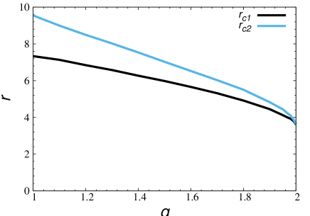
Figure 7: Marginal dimensions $r_{c1}$ (lower curve) and $r_{c_{2}}$ (upper curve) for the Potts model at $1\leq q\leq 2$. At $q=2$ both $r_{c1}$ and $r_{c_{2}}$ coincide within the fidelity interval: $r_{c1}=r_{c2}\simeq 3.65(5)$.

In the limiting case $q\to 1$, Eq. (12) gives the free energy that depends on the second-order parameter $m_{2}$ only:

$$\lim_{q\to 1}f(m_{1},m_{2})=\frac{z\left(m_{2}r+1\right)^{2}}{2(r+1)^{2}}-T\log\left(e^{\frac{h+\frac{z(m_{2}r+1)}{r+1}}{T}}+r\right).$$ (19)

Minimizing the free energy with respect to $m_{2}$ one gets the temperature behaviour $m_{2}(T)$. In turn, the appearance of a gap in this dependence can be used as a condition to determine the marginal dimension $r=r_{c1}$. We estimate numerically the marginal dimension $r_{c2}$ from the limit $\lim_{q\to 1^{+}}r_{c2}(q)$.

4 Conclusions

In this paper, we reconsidered the mean field approach to the recently introduced Potts model with invisible states [16]. The model was suggested in an attempt to resolve controversies between theoretical predictions of a second-order phase transition and simulations indicating a first-order scenario [17]. Indeed, the number of invisible states $r$ introduced into the model plays the role of a parameter that regulates the order of the phase transition. In the Potts case with $q$ interacting (visible) states, the transition becomes the first order starting from a certain, marginal, value $r_{c}$. For the particular case $q=2$ it had already been shown that the change occurs at large $r$ (for $d=2$) and that $3<r_{c}<4$ within the mean field analysis [16, 19]. Here, we determine a more precise estimate for the value for $q=2$, namely $r_{c}\simeq 3.65(5)$. This estimate is in excellent agreement with the $z\to\infty$ limit of the result obtained for the Bethe lattice with $z$ nearest neighbours [25].

We then considered the region $1\leq q<2$. There, the mechanism which changes the order of the phase transition is, to our knowledge, new to the field. Namely, there are two marginal dimensions, $r_{c1}$ and $r_{c2}$, as indicated in Fig. 4a, b. They characterise the temperature behaviour of the first derivatives of the free energy. At $r_{c1}$ the gap appears at a certain temperature $\tilde{t}<t_{c}$, however, the transition at $t_{c}$ remains of second order. The gap increases and moves towards $t_{c}$ with further increase of $r$, and, finally at $r_{c2}$ it reaches $t_{c}$: the transition becomes the first order. The marginal dimensions $r_{c1}$ and $r_{c2}$ are functions of $q$, they are shown in Fig. 7 and listed in Table 2.

The above observations shows essential difference in behaviour of the Potts model with invisible states at $q=2$ and at $1\leq q<2$. Whereas in the former case an increase of $r$ turns the second-order phase transition to the weak first-order transition (the jump in the order parameter $\lim_{r\to r_{c}}\Delta m_{1}\to 0$), in the latter case the second transition is turned to the sharp first-order transition, $\lim_{r\to r_{c2}}\Delta m_{1}\neq 0$. The same conclusion can be reached analysing the latent heat behaviour. In this respect, it is worth recalling that the case $q=1$, considered here, corresponds to the bond percolation. In turn, our result means that adding invisible states turns transition in the bond-percolation model into strong first-order. It is also worth mentioning here other mechanisms that are known to sharpen percolation transitions, such as those delivering explosive [38, 39] or bootstrap [40] percolation.

Marginal dimensions are widely met when phase transitions are analysed. Some examples are mentioned in the beginning of this paper. The first step towards defining these quantities for the Potts model with invisible states have been taken. More involved theories have to take into account fluctuations, which are wiped out within the method we currently used. One such approach, the renormalization group, leads to a perturbative expansion where the mean-field result enters as a first term. It is instructive to note here, that already this first-order contribution is non-integer, as foreseen by the results of this paper. Moreover, usually one expects logarithmic corrections to scaling to accompany the change in the order of a phase transition [41]. Again, these topics are out of reach of the mean-field analysis and will be a subject of a separate study.

This work was supported in part by FP7 EU IRSES projects No. $295302$ “Statistical Physics in Diverse Realizations”, No. $612707$ “Dynamics of and in Complex Systems”, No. $612669$ “Structure and Evolution of Complex Systems with Applications in Physics and Life Sciences”, and by the Doctoral College for the Statistical Physics of Complex Systems, Leipzig-Lorraine-Lviv-Coventry $({\mathbb{L}}^{4})$.

References

References

- [1] Stanley H E (1988) Introduction to Phase Transitions and Critical Phenomena (International Series of Monographs on Physics) (Oxford Science Publications, Oxford)
- [2] Domb C, The Critical Point (Taylor & Francis, London, 1996)
- [3] Stanley H E 1969 Phys. Rev. 179 570
- [4] Mermin N D and Wagner H 1966 Phys. Rev. Lett. 17 1133
- [5] Hohenberg P C 1967 Phys. Rev. 158 383
- [6] Aharony A 1976, in Phase Transitions and Critical Phenomena, edited by Domb C and Green M S, Academic Press, London 6
- [7] Sznajd J 1984 J. Magn. Magn. Mater. 42 269; Domański Z and Sznajd J 1985 Phys. Status Solidi B 129 135
- [8] Kleinert H and Schulte-Frohlinde V 1995 Phys. Lett. B 342 284; Folk R, Holovatch Yu, and Yavors’kii T 2000 Phys. Rev. B 62 12195, Erratum Phys. Rev. B 63 189901(E)
- [9] Dudka M, Holovatch Yu, and Yavors’kii T 2004 J. Phys. A: Math. Gen. 37 10727
- [10] Potts R B 1952 Proc. Camb. Phil. Soc. 48 106
- [11] Wu F Y 1982 Rev. Mod. Phys. 54 23
- [12] Holovatch Yu, Ivaneyko D, and Delamotte B 2004 J. Phys. A: Math. Gen. 37 3569
- [13] Delamotte B, Mouhanna D, and Tissier M 2004 Phys. Rev. B 69 134413; Calabrese P and Parruccini P 2004 Nucl. Phys. B 679 568
- [14] Pelissetto A and Vicari E 2002 Phys. Rep. 368 549; Folk R, Holovatch Yu, and Yavors’kii T 2003 Physics-Uspiekhi 46 169
- [15] Halperin B I, Lubensky T C, and Ma S 1974 Phys. Rev. Lett. 32 292; Folk R and Holovatch Yu 1996 J. Phys. A: Math. Gen 29 3409; Dudka M, Folk R, Holovatch Yu, and Moser G 2012 Condens. Matter Phys. 15 43001
- [16] Tamura R, Tanaka S, and Kawashima N 2010 Prog. Theor. Phys. 124 381
- [17] Tamura R and Kawashima N 2008 J. Phys. Soc. Jpn. 77 103002; Stoudenmire E M, Trebst S, and Balents L 2009 Phys. Rev. B 79 214436; Okumura S, Kawamura H, Okubo T, and Motome Y 2010 J. Phys. Soc. Jpn. 79 114705
- [18] Tanaka S, Tamura R, and Kawashima N 2011 J. Phys.: Conf. Ser. 297 012022
- [19] Tamura R, Tanaka S, and Kawashima N 2011 arXiv:1111.6509
- [20] Johnston D A and Ranasinghe R P K C M 2013 J. Phys. A: Math. Theor. 46 225001
- [21] Tanaka S and Tamura R 2011 J. Phys.: Conf. Ser. 320 012025
- [22] Mori T 2012 J. Stat. Phys. 147 1020
- [23] van Enter A C D, Iacobelli G, and Taati S 2011 Prog. Theor. Phys. 126 983
- [24] van Enter A C D, Iacobelli G, and Taati S 2011 arXiv:1109.0189
- [25] Ananikian N, Izmailyan N Sh, Johnston D A, Kenna R, and Ranasinghe R P K C M 2013 J. Phys. A: Math. Theor. 46 385002
- [26] Kihiara T, Midzuno Y, and Shizume J 1954 J. Phys. Soc. Jpn. 9 681; Mittag L and Stephen J 1974 J. Phys. A: Math. Gen. 7 L109; Straley J P and Fisher M E 1973 J. Phys. A: Math. Gen. 6 1310
- [27] Kasteleyn P W and Fortuin C M 1969 J. Phys. Soc. Jpn. 26 (Suppl.) 11
- [28] Giri M R, Stephen M J, and Grest G S 1977 Phys. Rev. B 16 4971
- [29] Stephen M J 1976 Phys. Lett. A 56 149
- [30] Deng Y, Garoni T M, and Sokal A D 2007 Phys. Rev. Lett. 98 030602
- [31] Jacobsen J L and Saleur H 2005 Nucl. Phys. B 716 439
- [32] Fortuin C M and Kasteleyn P W 1972 Physica 57 536
- [33] Stenull O, Janssen H K, and Oerding K 1999 Phys. Rev. E 59 4919
- [34] Aharony A 1978 J. Phys. C: Solid State Phys. 11
- [35] Aharony A and Pfeuty P 1979 J. Phys. C: Solid State Phys. 12
- [36] Siva K, Tao J, and Marcolli M 2015 arXiv: 1508.00504
- [37] Lubensky T C and Isaacson J 1978Phys. Rev. Lett. 41 12
- [38] Achlioptas D, D’Souza R M, and Spencer J 2009 Science 323 5920
- [39] Bastas N, Giazitzidis P, Maragakis M, and Kosmidis K 2014 Physica A 407 54
- [40] Adler J 1991 Physica A 171 453
- [41] Kenna R 2013 in: Order, Disorder and Criticality vol 3), ed. Holovatch Yu (Singapore: World Scientific) pp 1-46