Limitations of sum of products of Read-Once Polynomials

Abstract

We study limitations of polynomials computed by depth two circuits built over read-once polynomials (ROPs) and depth three syntactically multi-linear formulas. We prove an exponential lower bound for the size of the $\Sigma\Pi^{[N^{1/30}]}$ arithmetic circuits built over syntactically multi-linear $\Sigma\Pi\Sigma^{[N^{8/15}]}$ arithmetic circuits computing a product of variable disjoint linear forms on $N$ variables. We extend the result to the case of $\Sigma\Pi^{[N^{1/30}]}$ arithmetic circuits built over ROPs of unbounded depth, where the number of variables with $+$ gates as a parent in an proper sub formula is bounded by $N^{1/2+1/30}$. We show that the same lower bound holds for the permanent polynomial. Finally we obtain an exponential lower bound for the sum of ROPs computing a polynomial in ${\sf VP}$ defined by Raz and Yehudayoff [18].

Our results demonstrate a class of formulas of unbounded depth with exponential size lower bound against the permanent and can be seen as an exponential improvement over the multilinear formula size lower bounds given by Raz [14] for a sub-class of multi-linear and non-multi-linear formulas. Our proof techniques are built on the one developed by Raz [14] and later extended by Kumar et. al. [10] and are based on non-trivial analysis of ROPs under random partitions. Further, our results exhibit strengths and limitations of the lower bound techniques introduced by Raz [14].

1 Introduction

More than three decades ago, Valiant [21] developed the theory of Algebraic Complexity classes based on arithmetic circuits as the model of algebraic computation. Valiant considered the permanent polynomial ${{\sf perm}}_{n}$ defined over an $n\times n$ matrix $X=(x_{i,j})_{1\leq i,j\leq n}$ of variables:

${\sf perm}_{n}(X)=\sum\limits_{\pi\in{S}_{n}}\prod\limits_{i=1}^{n}x_{i,\pi(i)},$

where $S_{n}$ is the set of all permutations on $n$ symbols. Valiant [21] showed that the polynomial family $({\sf perm}_{n})_{n\geq 0}$ is complete for the complexity class ${\sf VNP}$. Further, Valiant [21] conjectured that ${{\sf perm}}_{n}$ does not have polynomial size arithmetic circuits. Since then, obtaining super polynomial size lower bounds for arithmetic circuits computing ${\sf perm}_{n}$ has been a pivotal problem in Algebraic Complexity Theory. However, for general classes of arithmetic circuits, the best known lower bound is quadratic in the number of variables [13].

Naturally, the focus has been on proving lower bound for ${\sf perm}_{n}$ against restricted classes of circuits. Grigoriev and Karpinski [3] proved an exponential size lower bound for depth three circuits of constant size over finite fields. Agrawal and Vinay [1] (See also [20, 9]) showed that proving exponential lower bounds against depth four arithmetic circuits is enough to resolve Valiant’s conjecture, and hence explaining the lack of progress in extending the results in [3] to higher depth circuits. This was strengthened to depth three circuits over infinite fields by Gupta et. al. [4].

Recently, Gupta et. al. [5] obtained a $2^{\Omega(\sqrt{n}\log n)}$ size lower bound for homogeneous depth four circuits computing ${\sf perm}_{n}$ where the bottom fan-in is bounded by $O(\sqrt{n})$. The techniques introduced in [5, 6] have been generalized and applied to prove lower bounds against various classes of constant depth arithmetic circuits, regular arithmetic formulas and homogeneous arithmetic formulas. (See e.g., [7, 11, 8].) Exhibiting polynomials that have exponential lower bound against concrete classes of arithmetic circuits is an important research direction.

In 2004, Raz [14] showed that any multilinear formula computing ${\sf perm}_{n}$ requires size $n^{\Omega(\log n)}$, which was one of the first super polynomial lower bounds against formulas of unbounded depth. Further, in [15], Raz extended this to separate multilinear formulas from multilinear circuits. Raz’s work lead to several lower bound results, most significant being an exponential separation of constant depth multilinear circuits [18]. More recently, Kumar et. al [10] extended the techniques developed in [14] to prove lower bounds against non-multilinear circuits and formulas.

•

Motivation and our Model : Depth three $\Sigma\Pi\Sigma$ circuits are in fact $\Sigma\Pi$ circuits built over linear forms. A linear form can be seen as the simplest form of read-once formulas (${\sf ROF}$): formulas where a variable appears at most once as a leaf label. Polynomials computed by ${\sf ROF}$s are called read-once polynomials or ${\sf ROP}$s. There are two natural generalizations of the $\Sigma\Pi\Sigma$ model: 1) Replace linear forms by sparse polynomials, this leads to the well studied $\Sigma\Pi\Sigma\Pi$ circuits; and 2) Replace linear forms with more general read-once formulae, this leads to the class of $\Sigma\Pi$ circuits over read-once formulas or $\Sigma\Pi{\sf ROP}$ for short.

In this paper, we consider the second extension, i.e., $\Sigma\Pi{\sf ROP}$. Restricted forms of $\Sigma\Pi{\sf ROP}$ were already considered in the literature. For example, Shpilka and Volkovich [19] obtained identity testing algorithms for the sum of ${\sf ROP}$s. Further [12] gives identity tests for $\Sigma\Pi{\sf ROP}$ when the top fan-in is restricted to two.

Apart from being a natural generalization of $\Sigma\Pi\Sigma$ circuits, the class $\Sigma\Pi{\sf ROP}$ can be seen as building non-multi-linear polynomials using the simplest possible multi-linear polynomials viz. ${\sf ROP}$s.

•

Our Results : We study the limitations of the model $\Sigma\Pi{\sf ROP}$ for some restricted class of circuits. Firstly, we prove,

Theorem 1.

Let $f_{i,j}$ be $N$-variate $\Sigma\Pi\Sigma$ syntactic multi-linear formulas with bottom $\Sigma$-fan-in at most $N^{1/2+\lambda}$ where $\lambda\leq 1/30$, and top $\Sigma$-fan-in at most $s^{\prime}$ for $1\leq i\leq s$ and $1\leq j\leq t$. Also assume that $t\leq N^{1/30}$. There is a product of variable disjoint linear forms $p_{lin}$ such that, if $\sum_{i}\prod_{j}f_{i,j}=p_{lin}$ then $s\cdot s^{\prime}=2^{\Omega(N^{1/4})}$.

Our arguments do not directly generalize to the case of unbounded depth ${\sf ROP}$s with small bottom $\Sigma$ fan-in. Nevertheless, we obtain a generalization of Theorem 1, allowing ${\sf ROP}$s of unbounded depth with a more stringent restriction than bottom $\Sigma$-fan-in. Let $F$ be an ${\sf ROF}$ and for a gate $v$ in $F$, let ${\sf sum\mbox{-}fan\mbox{-}in}(v)$ be the number of variables in the sub-formula rooted at $v$ whose parents are labelled as $+$. Then $s_{F}$ is the maximum value of ${\sf sum\mbox{-}fan\mbox{-}in}(v)$, where the maximum is taken over all $+$ gates in $F$ excluding the top layer of $+$ gates. Note that, in the case of $\Sigma\Pi\Sigma$ ${\sf ROP}$s, $s_{F}$ is equivalent to the bottom fan-in. For an ${\sf ROP}$ $f$, $s_{f}$ is the smallest value of $s_{F}$ among all ${\sf ROF}$s $F$ computing $f$. We prove,

Theorem 2.

Let $f_{i,j}$ be ${\sf ROP}$s with $s_{f_{i,j}}\leq N^{1/2+\lambda}$ for $\lambda\leq 1/30$, $1\leq i\leq s$ and $1\leq j\leq t$, where $t\leq N^{1/30}$. There is a product of linear forms ${p_{lin}}$ such that, if $\sum_{i}\prod_{j}f_{i,j}={p_{lin}}$ then $s=2^{\Omega(N^{1/4})}$.

As far as we know, this is the first exponential lower bound for a sub-class of non-multi-linear formulas of unbounded depth. It can be noted that our result above does not depend on the depth of the ${\sf ROP}$s. Further, note that even though a product of linear forms is a simple linear projection of ${\sf perm}_{n}$, Theorem 2 does not imply a lower bound for ${\sf perm}_{n}$ due to restrictions on $s_{F}$, since linear projections might change the bottom fan-in of the resulting ${\sf ROP}$s. However, we prove,

Theorem 3.

Let $f_{i,j}$ be ${\sf ROP}$s with $s_{f_{i,j}}\leq N^{1/2+\lambda}$ for $\lambda\leq 1/30$, $1\leq i\leq s$ and $1\leq j\leq t$, for $N=n^{2}$ and $t\leq N^{1/30}$. Then, if $\sum_{i}\prod_{j}f_{i,j}={\sf perm}_{n}$ then $s=2^{\Omega(N^{\epsilon})}$ for some $\epsilon>0$.

Finally, we show that the polynomial $g$ defined by Raz-Yehudayoff [17] cannot be written as sum of sub-exponentially many ${\sf ROP}$s:

Theorem 4.

There is a polynomial $g\in{\sf VP}$ such that for any ${\sf ROP}$s $f_{1},\ldots,f_{s}$, if $\sum_{i}f_{i}=g$, then we have $s=2^{\Omega(n/\log n)}$.

Related Results : Shpilka and Volkovich [19] proved a linear lower bound for a special class of ${\sf ROP}$s to sum-represent the polynomial $x_{1}\cdots x_{n}$ and used it crucially in their identity testing algorithm. Theorem 4 is an exponential lower bound against the same model as in [19], however against a polynomial in ${\sf VP}$. It should be noted that the results in Raz [14] combined with [10] immediately implies a lower bound of $n^{\Omega(\log n)}$ for the sum of ${\sf ROP}$s. Our results are an exponential improvement of bound given by [14].

Kayal [6] showed that at least $2^{n/d}$ many polynomials of degree $d$ are required to represent the polynomial $x_{1}\dots x_{n}$ as sum of powers. Our model is significantly different from the one in  [6] since it includes high degree monomials, though the powers are restricted to be sub-linear, whereas Kayal’s argument works against arbitrary powers.

•

Our Techniques Our techniques are broadly based on the partial derivative matrix technique introduced by Raz [14] and later extended by Kumar et. al [10]. It can be noted that the lower bounds obtained in [14] are super polynomial and not exponential. Though Raz-Yehudayoff [18] proved exponential lower bounds, their argument works only against bounded depth multilinear circuits. Further, the arguments in [14, 18] do not work for the case of non-multilinear circuits, and fail even in the case of products of two multilinear formulas. This is because rank of the partial derivative matrix, a complexity measure used by [14, 18] (see Section 2 for a definition) is defined only for multi-linear polynomials. Even though this issue can be overcome by a generalization introduced by Kumar et. al [10], the limitation lies in the fact that the upper bound of $2^{n-n^{\epsilon}}$ for an $n^{2}$ or $2n$ variate polynomial, obtained in [14] or [18] on the measure for the underlying arithmetic formula model is insufficient to handle products of two ${\sf ROP}$s.

Our approach to prove Theorems 2 and 3 lie in obtaining an exponentially stronger upper bounds (see Lemma 17 ) on the rank of the partial derivative matrix of an ${\sf ROP}$ $F$ on $N$ variables where $s_{F}\leq N^{1/2+1/30}$. Our proof is a technically involved analysis of the structure of ${\sf ROP}$s under random partitions of the variables. Even though the restriction on $s_{F}$ might look un-natural, in Lemma 18, we show that a simple product of variable disjoint linear forms in $N$-variables, with $s_{F}\geq N^{2/3}$ achieve exponential rank with probability $1-2^{-\Omega(N^{1/3})}$. Thus our results highlight the strength and limitations of the techniques developed in [18, 10] to the case of non-multi-linear formulas.

Finally proof of Theorem 4 is based on an observation pointed out to the authors by an anonymous reviewer. We have included it here since the details have been worked out completely by the authors.

Due to space limitations, all the missing proofs can be found in Sections 5,6 and 7.

2 Preliminaries

Let $\mathbb{F}$ be an arbitrary field and $X=\{x_{1},\ldots,x_{N}\}$ be a set of variables. An arithmetic circuit $\mathcal{C}$ over $\mathbb{F}$ is a directed acyclic graph with vertices of in-degree 0 or 2 and exactly one vertex of out-degree 0 called the output gate. The vertices of in-degree 0 are called input gates and are labeled by elements from $X\cup\mathbb{F}$. The vertices of in-degree more than 0 are labeled by either $+$ or $\times$. Thus every gate of the circuit naturally computes a polynomial. The polynomial $f$ computed by $\mathcal{F}$ is the polynomial computed by the output gate of the circuit.

An arithmetic formula is a an arithmetic circuit $\mathcal{F}$ where every gate has out-degree bounded by $1$, i.e., the underlying undirected graph $\mathcal{F}$ is a tree.

The size of an arithmetic circuit $\mathcal{F}$ is the number of gates in $\mathcal{F}$. For any gate $v$ depth of $v$ is the length of the longest path from an input gate to $v$ gate in $\mathcal{F}$. Depth of $\mathcal{F}$ is defined as the depth of its output gate.

An arithmetic read-once formula (${\sf ROF}$ for short) is an arithmetic formula $\mathcal{F}$ over $X$ where every input variable $x\in X$ occurs as a label of at most once $\mathcal{F}$. The polynomial $f$ computed by an ${\sf ROF}$ $\mathcal{F}$ is called a read-once-polynomial or ${\sf ROP}$.

Let $f(y_{1},\ldots,y_{m},z_{1},\ldots,z_{m})\in\mathbb{F}[y_{1},\ldots,y_{m},z_{1},\ldots,z_{m}]$ be a multilinear polynomial. The partial derivative matrix of $f$ denoted by $M_{f}$ [14] is a $2^{m}\times 2^{m}$ matrix defined as follows: The rows of $M_{f}$ are labeled by all possible multilinear monomials in $\{y_{1},\ldots,y_{m}\}$ and the columns of $M_{f}$ be labeled by all possible multilinear monomials in $\{z_{1},\ldots,z_{m}\}$. For any two multilinear monomials $p$ and $q$, the entry $M_{f}[p,q]$ is the coefficient of $p\cdot q$ in $f$.

Lemma 1.

[16](Sub-Additivity.) Let $f=f_{1}+f_{2}$ where $f,f_{1}$ and $f_{2}$ are multilinear polynomials in $\mathbb{F}[y_{1},\ldots,y_{m},z_{1},\ldots,z_{m}]$. Then, $rank(M_{f})\leq rank(M_{f_{1}})+rank(M_{f_{2}}).$ Moreover, if $\sf var(f_{1})\cap\sf var(f_{2})=\emptyset$ then $rank(M_{f})=rank(M_{f_{1}})+rank(M_{f_{2}}).$

Lemma 2.

[16](Sub-Multiplicativity.) Let $f=f_{1}\times f_{2}$, where $f,f_{1}$ and $f_{2}$ are multilinear polynomials in $\mathbb{F}[y_{1},\ldots,y_{m},z_{1},\ldots,z_{m}]$, and $\sf var(f_{1})\cap\sf var(f_{2})=\emptyset$. Then, $rank(M_{f})=rank(M_{f_{1}})\cdot rank(M_{f_{2}}).$

Kumar et. al. [10] generalized the notion of partial derivative matrix to include polynomials that are not multilinear. Let $Y=\{y_{1},\ldots,y_{m}\}$ and $Z=\{z_{1},\ldots,z_{m}\}$. Let $f\in\mathbb{F}[Y,Z]$ be a polynomial. The polynomial coefficient matrix of $f$ denoted by $\widehat{M}_{f}$ is a $2^{m}\times 2^{m}$ matrix defined as follows. For multilinear monomials $p$ and $q$ in variables $Y$ and $Z$ respectively, the entry $\widehat{M}_{f}[p,q]=A$ if and only if $f$ can be uniquely expressed as $f=pq\cdot A+B$ where $A,B\in\mathbb{F}[Y,Z]$ such that $\sf var(A)\subseteq\sf var(p)\cup\sf var(q)$ and $B$ does not have any monomial that is divisible by $p\cdot q$ and contains only variables present in $p$ and $q$.

Observation 1.

[10] For a multilinear polynomial $f\in\mathbb{F}[Y,Z]$, we have $\widehat{M}_{f}=M_{f}$.

Observe that the matrix $\widehat{M}_{f}$ has polynomial entries. Therefore $\operatorname{rank}(\widehat{M}_{f})$ is defined only under a substitution function that substitutes every variable in $f$ to a field element.

For any substitution function $S:Y\cup Z\rightarrow\mathbb{F}$, let us denote by ${\widehat{M}_{f}}|_{S}$ the matrix obtained by substituting every variable in $f$ at each entry of $\widehat{M}_{f}$ to the field element given by $S$. Define, $\operatorname{maxrank}(\widehat{M}_{f})\triangleq\max\limits_{S:Y\cup Z\rightarrow\mathbb{F}}\operatorname{rank}({\widehat{M}_{f}}|_{S}).$ Having defined polynomial coefficient matrix $\widehat{M}_{f}$ and $\operatorname{maxrank}(\widehat{M}_{f})$ we now look at properties of $\widehat{M}_{f}$ with respect to $\operatorname{maxrank}$.

Lemma 3.

[10](Sub-additivity.) Let $f,g\in\mathbb{F}[Y,Z]$. Then, $\operatorname{maxrank}(\widehat{M}_{f+g})\leq\operatorname{maxrank}(\widehat{M}_{f})+\operatorname{maxrank}(\widehat{M}_{g}).$

Lemma 4.

[10](Sub-multiplicativity.) Let $Y_{1},Y_{2}\subseteq Y$ and $Z_{1},Z_{2}\subseteq Z$ such that $Y_{1}\cap Y_{2}=\emptyset$ and $Z_{1}\cap Z_{2}=\emptyset$. Then for any polynomials $f\in\mathbb{F}[Y_{1},Z_{1}]$, $g\in\mathbb{F}[Y_{2},Z_{2}]$ we have: $\operatorname{maxrank}(\widehat{M}_{fg})=\operatorname{maxrank}(\widehat{M}_{f})\cdot\operatorname{maxrank}(\widehat{M}_{g})$.

A partition of $X$ is a function $\varphi:X\rightarrow Y\cup Z\cup\{0,1\}$ such that $\varphi$ is an injection when restricted to $Y\cup Z$, i.e., $\forall x\neq x^{\prime}\in X$, if $\varphi(x)\in Y\cup Z$ and $\varphi(x^{\prime})\in Y\cup Z$ then $\varphi(x)\neq\varphi(x^{\prime})$. Let $F$ be an ${\sf ROF}$ and $\varphi:X\rightarrow Y\cup Z\cup\{0,1\}$ be a partition function. Define $F^{\varphi}$ to be the formula obtained by replacing every variable $x$ that appears as a leaf in $F$ by $\varphi(x)$. Then the polynomial $f^{\varphi}$ computed by $F^{\varphi}$ is $f^{\varphi}=f(\varphi(x_{1}),\ldots,\varphi(x_{n}))$. Observe that $f^{\varphi}\in\mathbb{F}[Y,Z]$.

An arithmetic formula $\mathcal{F}$ is said to be a constant-minimal formula if no gate $u$ in $F$ has both its children to be constants. Observe that for any arithmetic formula $F$, if there exists a gate $u$ in $F$ such that $u=a~{}{\sf op}~{}b,a,b\in\mathbb{Z}$ then we can replace $u$ in $F$ by the constant $a~{}{\sf op}~{}b$, where ${\sf op}\in\{+,-\}$. Thus we assume without loss of generality that $\mathcal{F}$ is constant-minimal.

We need some observations on formulas that compute natural numbers. Recall that an arithmetic formula $\mathcal{F}$ is said to be monotone if $\mathcal{F}$ does not contain any negative constants.

Let $G$ be a monotone arithmetic formula were the leaves are labeled numbers in $\mathbb{N}$. Then for any gate $v$ in $G$, the value of $v$ denoted by ${\sf value}(v)$ is defined as : If $u$ is a leaf then ${\sf value}(u)=a$ where $a\in\mathbb{N}$ is the label of $u$ and $u=u_{1}~{}{\sf op}~{}u_{2}$ then ${\sf value}(u)={\sf value}(u_{1})~{}{\sf op}~{}{\sf value}(u_{2})$, where ${\sf op}\in\{+,\times\}$. Finally, ${\sf value}(G)$ is the value of the output gate of $G$. Let $G$ be a monotone arithmetic formula with leaves labelled by either $1$ or $2$. A node $u$ a is called a $rank\text{-}(1,2)\text{-}separator$ if $u$ is a leaf and ${\sf value}(u)=2$ or $u=u_{1}+u_{2}$ with ${\sf value}(u)=2$ and ${\sf value}(u_{1})={\sf value}(u_{2})=1$. The following is a simple upper bound on the value computed by a formula.

Lemma 5.

Let $G$ be a binary monotone arithmetic formula with $t$ leaves. If every leaf in $G$ takes a value at most $N>1$, then ${\sf value}(G)\leq N^{t}$.

Proof.

The proof is by induction on the size of the formula. Base Case : $s=1$

• If $G$ has a single $+$ gate then $\c@(G)\leq N+N\leq N^{2}$.

• If $G$ has a single $\times$ gate then $\c@(G)\leq N\cdot N=N^{2}$.

Induction Step : Let $u$ be the output gate of $G$ with children $u_{1}$ and $u_{2}$. Let the number of leaves in the sub formula rooted at $u_{1}$ and $u_{2}$ be $t_{1}$ and $t_{2}$.

• If $u$ is a $+$ gate. Then, ${\sf value}(u)={\sf value}(u_{1})+{\sf value}(u_{2})$. By induction hypothesis, ${\sf value}(u)\leq N^{t_{1}}+N^{t_{2}}\leq N^{t_{1}+t_{2}}\leq N^{t}$.

• If $u$ is a $\times$ gate. Then, ${\sf value}(u)={\sf value}(u_{1})\times{\sf value}(u_{2})$. By induction hypothesis, ${\sf value}(u)\leq N^{t_{1}}\times N^{t_{2}}\leq N^{t_{1}+t_{2}}\leq N^{t}$.

∎

Any formula with a large value should have a large number of $rank\text{-}(1,2)\text{-}separator$s.

Lemma 6.

Let $F$ be a binary monotone arithmetic formula with leaves labeled by either $1$ or $2$. If ${\sf value}(F)>2^{r}$ then there exists at least $\frac{r}{\log N}$ nodes that are $rank\text{-}(1,2)\text{-}separator$s.

Proof.

Let $F$ be a binary monotone arithmetic formula with leaves labeled by either $1$ or $2$. First mark every node $u$ such that $u$ is a $rank\text{-}(1,2)\text{-}separator$ and remove sub-formula rooted at $u$ except $u$. Consider any leaf $v$ that remains unmarked and along the path from $v$ to root there is no node that is marked. Then ${\sf value}(v)=1$. Consider the unique path from $v$ to root in $F$. Let $p$ the first node in the path such that ${\sf value}(p)\geq 2$. Let $p_{1}$ and $p_{2}$ be the children of $p$. Without loss of generality let $p_{1}$ be an ancestor of $v$. Then observe that there is atleast one marked node(say $q$) in the sub-formula rooted at $p_{2}$. Set ${\sf value}(q)={\sf value}(q)+1$. If $p$ is a $+$ gate set $p_{1}=0$ else set $p_{1}=1$. Let $u_{1},\ldots,u_{t}$ be the leaves of the resulting formula at the end of this process. For every $1\leq i\leq t$, we have $2\leq{\sf value}(u_{i})\leq N$. Therefore by Lemma 5, ${\sf value}(F)\leq N^{t}$. Since ${\sf value}(F)>2^{r}$, we have $2^{r}<N^{t}$. Therefore $t>\frac{r}{\log N}$ as required. ∎

Finally, we will use the following variants of Chernoff-Hoeffding bounds.

Theorem 5.

[2](Chernoff-Hoeffding bound) Let $X_{1},X_{2},\ldots,X_{n}$ be independent random variables. Let $X=X_{1}+X_{2}+\cdots+X_{n}$ and $\mu=\mathbb{E}[X]$. Then for any $\delta>0$,

• $\Pr[X>(1+\delta)\mu]<\left(\frac{\mathrm{e}^{\delta}}{(1+\delta)^{(1+\delta)}}\right)^{\mu}$; and

• $\Pr[X\geq(1+\delta)\mu]\leq\mathrm{e}^{\frac{-\delta^{2}\mu}{3}}$; and

• $\Pr[X\leq(1-\delta)\mu]\leq\mathrm{e}^{\frac{-\delta^{2}\mu}{2}}$.

3 Hardness of representation for Sum of ${\sf ROP}$s

Let $X=\{x_{1},\ldots,x_{2n}\},Y=\{y_{1},\ldots,y_{2n}\},Z=\{z_{1},\ldots,z_{2n}\}$. Define $\cal{D^{\prime}}$ as a distribution on the functions $\varphi:X\to Y\cup Z$ as follows : For $1\leq i\leq 2n$,

$\varphi(x_{i})\in\begin{cases}Y&\mbox{with prob. }\frac{1}{2}\\ Z&\mbox{with prob. }\frac{1}{2}\end{cases}$

Observe that $|\varphi(X)\cap Y|=|\varphi(X)\cap Z|$ is not necessarily true. Let $F$ be a binary arithmetic formula computing a polynomial $f$ on the variables $X=\{x_{1},\ldots,x_{2n}\}$. Note that any gate with at least one variable as a child can be classified as:

• type-$A$ gates : sum gates both of whose children are variables,

• type-$B$ gates : product gates both of whose children are variables,

• type-$C$ gates : sum gates exactly one child of which is a variable and the other an internal gate; and

• type- $D$ gates: product gates exactly one child of which is a variable and the other an internal gate

Given any ${\sf ROF}$ $F$, let there be $a$ type-$A$ gates, $b$ type-$B$, $c$ type-$C$ and $d$ type-$D$ gates in $F$. Note that $2a+2b+c+d=2n$. Let $\varphi\sim\mathcal{D}^{\prime}$. Let there be $a^{\prime}$ gates of type-$A$ that achieve $\operatorname{rank}$-1 under $\varphi$ and let $a^{\prime\prime}$ gates of type-$A$ that achieve $\operatorname{rank}$-2 under $\varphi$. Then, $a=a^{\prime}+a^{\prime\prime}$.

Lemma 7.

Let $F$ be an ${\sf ROF}$ computing an ${\sf ROP}$ $f$ and $\varphi:X\to Y\cup Z$. Then, $\operatorname{rank}(M_{f^{\varphi}})\leq 2^{a^{\prime\prime}+\frac{a^{\prime}}{2}+{b}+\frac{c}{2}}.$

Proof.

Observe that for any type-$D$ gate $g=h\times x$, $\operatorname{rank}(M_{g^{\varphi}})=\operatorname{rank}(M_{{(x\cdot h)}^{\varphi}})=\operatorname{rank}(M_{h^{\varphi}})$, and hence type-$D$ gates do not contribute to the rank.

The proof is by induction on the structure of $F$. Base case is when $F$ is of depth 1. Let $r$ be the root gate of $F$ computing the polynomial $f$. Then

• $r$ is an type-$A$ gate with children $x_{1},x_{2}$ : $f=x_{1}+x_{2}$. For any $\varphi$, we have $\operatorname{rank}(M_{f^{\varphi}})\leq 2$. Then $a=1,b=0,c=0$. Therefore either $a^{\prime}=1$ or $a^{\prime\prime}=1$. In either case, $\operatorname{rank}(M_{f^{\varphi}})\leq 2^{a^{\prime\prime}+\frac{a^{\prime}}{2}+{b}}$.

• $r$ is a type-$B$ gate with children $x_{1},x_{2}$ : $f=x_{1}\cdot x_{2}$. For any $\varphi$ we have $\operatorname{rank}(M_{f^{\varphi}})\leq 1$. Then $a=0,b=1,c=0$. Therefore $\operatorname{rank}(M_{f^{\varphi}})\leq 2^{a^{\prime\prime}+\frac{a^{\prime}}{2}+{b}+\frac{c}{2}}$.

For the induction step, we have the following cases based on the structure of $f$.

• $r$ is a type-$C$ gate with children $x,h$, i.e., $f=h+x$. For any $\varphi$, we have by sub-additivity $\operatorname{rank}(M_{f^{\varphi}})\leq\operatorname{rank}(M_{h^{\varphi}})+\operatorname{rank}(M_{x^{\varphi}})$. Let $a_{h}^{\prime},a_{h}^{\prime\prime}$ be the number of type-$A$ gates in the sub-formula rooted at $h$ that achieve rank-1 and rank-2 under $\varphi$ respectively. Let $b_{h},c_{h}$ be the number of type-$B$ and $c$ type-$C$ gates in the sub-formula rooted at $h$. We now have $a^{\prime}=a_{h}^{\prime},a^{\prime\prime}=a_{h}^{\prime\prime},b=b_{h},c=c_{h}+1$, and $\operatorname{rank}(M_{f^{\varphi}})\leq\operatorname{rank}(M_{h^{\varphi}})+\operatorname{rank}(M_{x^{\varphi}}).$ By Induction hypothesis $\operatorname{rank}(M_{h^{\varphi}})\leq 2^{a_{h}^{\prime\prime}+\frac{a_{h}^{\prime}}{2}+b_{h}+\frac{c_{h}}{2}}$. First suppose the case when $a_{h}^{\prime\prime}+\frac{a_{h}^{\prime}}{2}+b_{h}+\frac{c_{h}}{2}\geq 1.5$, then, $\operatorname{rank}(M_{f^{\varphi}})\leq 2^{a_{h}^{\prime\prime}+\frac{a_{h}^{\prime}}{2}+b_{h}+\frac{c_{h}}{2}}+\operatorname{rank}(M_{x^{\varphi}})=2^{a_{h}^{\prime\prime}+\frac{a_{h}^{\prime}}{2}+b_{h}+\frac{c_{h}}{2}}+1\leq 2^{a^{\prime\prime}+\frac{a^{\prime}}{2}+{b}+\frac{c}{2}}$. Now suppose $a_{h}^{\prime\prime}+\frac{a_{h}^{\prime}}{2}+b_{h}+\frac{c_{h}}{2}<1.5$ and hence $a_{h}^{\prime\prime}+\frac{a_{h}^{\prime}}{2}+b_{h}+\frac{c_{h}}{2}\leq 1$ (since $a_{h}^{\prime\prime},a_{h},b_{h}$ and $c_{h}$ are integers). If $a_{h}^{\prime\prime}=1$, then $rank(M_{f^{\varphi}})=2<2^{a^{\prime\prime}+\frac{a^{\prime}}{2}+\frac{b}{2}+\frac{c}{2}}$. Finally, if $a_{h}^{\prime\prime}=0$, for all of the remaining possibilities, we have $\operatorname{rank}(M_{f^{\varphi}})\leq 2\leq 2^{a^{\prime\prime}+\frac{a^{\prime}}{2}+b+\frac{c}{2}}$.

• $r=g\times h$ be an internal gate. For $H\in\{g,h\}$, let $a_{H}^{\prime},a_{H}^{\prime\prime}$ be the number of type-$A$ gates that achieve rank-1 and rank-2 under $\varphi$ respectively and $b_{H},c_{H}$ be the number of type-$B$ and $c$ type-$C$ gates in the sub-formula rooted at $H$. Then $f=g*h$ where $*\in\{+,\times\}$. In either case, $\operatorname{rank}(M_{f^{\varphi}})\leq\operatorname{rank}(M_{g^{\varphi}})\cdot\operatorname{rank}(M_{h^{\varphi}})$, and from Induction hypothesis $\operatorname{rank}(M_{f^{\varphi}})\leq\cdot 2^{a_{g}^{\prime\prime}+\frac{a_{g}^{\prime}}{2}+{b_{g}}+\frac{c_{g}}{2}}2^{a_{h}^{\prime\prime}+\frac{a_{h}^{\prime}}{2}+b_{h}+\frac{c_{h}}{2}}.$ Since $a^{\prime}=a_{g}^{\prime}+a_{h}^{\prime},a^{\prime\prime}=a_{g}^{\prime\prime}+a_{h}^{\prime\prime},b=b_{h}+b_{g},c=c_{g}+c_{h}$ we have $\operatorname{rank}(M_{f^{\varphi}})\leq 2^{a^{\prime\prime}+\frac{a^{\prime}}{2}+b+\frac{c}{2}}.$

∎

Lemma 8.

Let $F$ be a ${\sf ROF}$ and $\varphi\sim\mathcal{D}^{\prime}$. Let $a^{\prime}$ be the number type-$A$ gates that achieve $\operatorname{rank}$-$1$ under $\varphi$. Then, $\Pr_{\varphi\sim\mathcal{D}^{\prime}}\left[\frac{2}{5}a\leq a^{\prime}\leq\frac{3}{5}a\right]\geq 1-2^{-\Omega(a)}.$

Proof.

Let $v$ be a type-$A$ gate in $F$. Then $f_{v}=x_{i}+x_{j}$ for some $i,j\in[N]$. Then $\Pr[\operatorname{rank}(M_{f_{v}^{\varphi}})=1]=\Pr[(\varphi(x_{i}),\varphi(x_{j})\in Z)\vee(\varphi(x_{i}),\varphi(x_{j})\in Y)]=\frac{1}{2}$. Therefore, $\mathbb{E}[a^{\prime}]=a/2$. Applying Theorem 5 (2) and (3) with $\delta=1/2$, we get the required bounds for $a^{\prime}$. ∎

Lemma 9.

Let $F$ be a ${\sf ROF}$ computing and ${\sf ROP}$ $f$ $2n$ variables, and $\varphi\sim{\cal D}^{\prime}$. Then with probability at least $1-2^{-\Omega(n)}$, $\operatorname{rank}(M_{f^{\varphi}})\leq 2^{n-\frac{n}{5\log n}}$.

Proof.

Consider the following two cases:
Case 1 : $a+c\geq\frac{2n}{\log n}$. Then either $a\geq\frac{n}{\log n}$ or $c\geq\frac{n}{\log n}$.
Firstly, suppose $a\geq\frac{n}{\log n}$, then by Lemma 1, we have $\operatorname{rank}(M_{f^{\varphi}})\leq 2^{a^{\prime\prime}+a^{\prime}/2+b+c/2}$. Since $2a^{\prime}+2a^{\prime\prime}+2b+c+d=2n$, we have $a^{\prime}/2+a^{\prime\prime}+b+c/2\leq n-a^{\prime}/2$. By Lemma 8, $a^{\prime}\geq 2/5a\geq 2n/5\log n$. Therefore, $\operatorname{rank}(M_{f\varphi})\leq 2^{a^{\prime\prime}+a^{\prime}/2+b+c/2}\leq 2^{n-a^{\prime}/2}\leq 2^{n-\frac{n}{5\log n}}$.
Now suppose $c\geq\frac{n}{5\log n}$. Since $2a^{\prime}+2a^{\prime\prime}+2b+c\leq 2n$, we have $a^{\prime\prime}+a^{\prime}+b+c/2\leq n-c/2\leq n-n/2\log n$. Therefore by Lemma 1, $\operatorname{rank}(M_{f^{\varphi}})\leq 2^{a^{\prime\prime}+a^{\prime}/2+b+c/2}\leq 2^{a^{\prime\prime}+a^{\prime}+b+c/2}\leq 2^{n-c/2}\leq 2^{n-\frac{n}{5\log n}}.$
Case 2 : $a+c<\frac{2n}{\log n}$. Observe that $b\leq n$. Since any type $B$ gate achieves rank 1 under any $\varphi$, by a simple inductive argument we have $\operatorname{rank}(M_{f^{\varphi}})\leq 2^{a+c+b/2}$ for any $\varphi$. Therefore $\operatorname{rank}(M_{f^{\varphi}})\leq 2^{a+c+b/2}\leq 2^{n/2+2n/\log n}\leq 2^{n-n/5\log n}.$ ∎

The following polynomial was introduced by Raz and Yehudayoff [17].

Definition 1.

Let $n\in\mathbb{N}$ be an integer. Let $X=\{x_{1},\ldots,x_{2n}\}$ and $\mathcal{W}=\{w_{i,k,j}\}_{i,k,j\in[2n]}$. For any two integers $i,j\in\mathbb{N}$, we define an interval $[i,j]=\{k\in\mathbb{N},i\leq k\leq j\}$. Let $|[i,j]|$ be the length of the interval $[i,j]$. Let $X_{i,j}=\{x_{p}\mid p\in[i,j]\}$ and $W_{i,j}=\{w_{i^{\prime},k,j^{\prime}}\mid i^{\prime},k,j^{\prime}\in[i,j]\}$. For every $[i,j]$ such that $|[i,j]|$ is even we define a polynomial $g_{i,j}\in\mathbb{F}[X,\mathcal{W}]$ as $g_{i,j}=1$ when $|[i,j]|=0$ and if $|[i,j]|>0$ then, $g_{i,j}\triangleq(1+x_{i}x_{j})g_{i+1,j-1}+\sum_{k}w_{i,k,j}g_{i,k}g_{k+1,j}.$ where $x_{k}$, $w_{i,k,j}$ are distinct variables, $1\leq k\leq j$ and the summation is over $k\in[i+1,j-2]$ such that the interval $[i,k]$ is of even length. Let $g\triangleq g_{1,2n}.$

In the following, we view $g$ as polynomial in $\{x_{1},\ldots,x_{2n}\}$ with coefficients from the rational function field $\mathbb{G}\triangleq\mathbb{F}(\mathcal{W})$.

Lemma 10.

Let Let $X=\{x_{1},\ldots,x_{2n}\}$, $Y=\{y_{1},\ldots,y_{2n}\}$, $Z=\{z_{1},\ldots,z_{2n}\}$ and $\mathcal{W}=\{w_{i,k,j}\}_{i,k,j\in[2n]}$ be sets of variables. Suppose $\varphi\sim\mathcal{D}^{\prime}$ such that $||\varphi(X)\cap Y|-|\varphi(X)\cap Z||=\ell$. Then for the polynomial $g$ as in Definition 1 we have, $\operatorname{rank}(M_{g^{\varphi}})\geq 2^{n-\ell/2}.$

Proof.

Proof builds on Lemma 4.3 in [17] as a base case and is by induction on $n+\ell$.

Base case: Either $\ell=0$ or $\ell=2n$. For $\ell=0$, the statement follows by Lemma 4.3 in [17]. When $\ell=2n$, then $\operatorname{rank}(M_{g^{\varphi}})=1=2^{n-\ell/2}$.

Induction step: Without loss of generality, assume that $|\varphi(X)\cap Y|=|\varphi(X)\cap Z|+\ell$. There are three possibilities:

Case 1 :

Let $\varphi(x_{1})\in Y$ and $\varphi(x_{2n})\in Z$ or vice versa. In this case

$$\operatorname{rank}(M_{g^{\varphi}}) \geq \operatorname{rank}(M_{(1+x_{1}x_{2n})^{\varphi}})\operatorname{rank}(M_{g_{2,2n-1}^{\varphi}})=2\cdot\operatorname{rank}(M_{g_{2,2n-1}^{\varphi}})$$

$$\geq 2\cdot 2^{n-1-\ell/2}=2^{{n-\ell/2}}\hskip 28.45274pt[\text{By Induction Hypothesis.}]$$

Case 2 :

$\varphi(x_{1})\in Y$ and $\varphi(x_{2n})\in Y$. Then

$$\operatorname{rank}(M_{g^{\varphi}}) \geq\operatorname{rank}(M_{(1+x_{1}x_{2n})^{\varphi}})\operatorname{rank}(M_{g_{2,2n-1}^{\varphi}})=1\cdot\operatorname{rank}(M_{g_{2,2n-1}^{\varphi}})$$

$$\geq 2^{(2n-2)/2-(\ell-2)/2}=2^{n-\ell/2}.\hskip 28.45274pt[\text{By Induction Hypothesis.}]$$

For the penultimate inequality above, note that $g_{2,2n-1}$ is defined on $X^{\prime}=\{x_{2},\ldots,x_{2n-1}\}$ and $||\varphi(X^{\prime})\cap Y|-|\varphi(X^{\prime})\cap Z||=\ell-2$ and hence by Induction Hypothesis, $\operatorname{rank}(M_{g_{2,2n-1}^{\varphi}})\geq 2^{(2n-2)/2-(\ell-2)/2}$.

Case 3

$\varphi(x_{1})\in Z$ and $\varphi(x_{2n})\in Z$. Then there is an $i\in\{2,2n-1\}$ such that $||\varphi(X_{i})\cap Y|-|\varphi(X_{i})\cap Z||=0$ and $||\varphi(X\setminus X_{i})\cap Y|-|\varphi(X\setminus X_{i})\cap Z||=\ell$, where $X_{i}=\{x_{1},\ldots,x_{i}\}$. Then by the definition of $g$, over $\mathbb{G}$, $\operatorname{rank}(M_{g^{\varphi}})\geq\operatorname{rank}(M_{g_{1,i}^{\varphi}})\cdot\operatorname{rank}(M_{g_{i+1,2n}^{\varphi}})\geq 2^{i/2}\cdot 2^{(2n-i)/2-\ell/2}=2^{n-\ell/2},$ since $\operatorname{rank}(M_{g_{1,i}^{\varphi}})=2^{i/2}$ by Lemma 4.3 in [17], and $\operatorname{rank}(M_{g_{i+1,2n}^{\varphi}})\geq 2^{(2n-i)/2-\ell/2}$ by Induction Hypothesis.

∎

Lemma 11.

$\Pr_{\varphi\sim{\cal D}^{\prime}}[n-n^{2/3}\leq|\varphi(X)\cap Y|\leq n+n^{2/3}]\geq 1-2^{-\Omega(n^{1/3})}$.

Proof.

Proof is a simple application of Chernoff’s bound (Theorem 5) with $\delta=1/n^{1/3}$. ∎

Corollary 1.

$\Pr_{\varphi\sim{\cal D}^{\prime}}[\operatorname{rank}(M_{g^{\varphi}})\geq 2^{n-n^{2/3}/2}]\geq 1-2^{-\Omega(n^{1/3})}$.

Proof.

Apply Lemma 10 with $\ell=n/n^{1/3}=n^{2/3}$ and the probability bound follows from Lemma 11. ∎

Proof of Theorem 4

Proof.

Suppose $s<2^{n/10\log n}$. Then by Lemma 9 and union bound, probability that there is an $i$ such that $\operatorname{rank}(M_{f_{i}^{\varphi}})\geq 2^{n-n/5\log n}$ is $s2^{-\Omega(n)}=2^{-\Omega(n)}$ and hence by Lemma 1, $\operatorname{rank}(M_{g^{\varphi}})\leq s2^{n-n/5\log n}\leq 2^{n-n/10\log n}$ with probability $1-2^{-\Omega(n)}$. However, by Corollary 1, $\operatorname{rank}(M_{g^{\varphi}})\geq 2^{n-n^{2/3}/2}>2^{n-n/10\log n}$ with probability at least $1-2^{-\Omega(n^{1/3})}$, a contradiction. Therefore, $s=2^{\Omega(n/\log n)}$. ∎

4 Sum of Products of ${\sf ROP}$s

4.1 ${\sf ROP}$s under random partition

Throughout the section, let $m\triangleq N^{1/3}$, $n\triangleq\sqrt{N}$ and $\kappa=20\log n$. Let $\cal{D}$ denote the distribution on the functions $\varphi:X\to Y\cup Z\cup\{0,1\}$ defined as follows

$\varphi(x_{ij})\in\begin{cases}Y&\mbox{with prob. }\frac{m}{N}\\ Z&\mbox{with prob. }\frac{m}{N}\\ 1&\mbox{with prob. }\frac{\kappa n}{N}\\ 0&\mbox{with prob. }1-\left(\frac{2m+\kappa n}{N}\right)\end{cases}$

Lemma 12.

Let $f$ be an ${\sf ROP}$ computed by an ${\sf ROF}$ $F$ and $\varphi\sim{\cal D}$. Let $X$ be a random variable that denotes the number of non-zero multiplication gates at depth $1$. Then $\Pr\limits_{\varphi\sim D}\left[X>\mathcal{O}(N^{1/6}\log n)\right]\leq 2^{-\Omega(m)}$.

Proof.

Consider a multiplication gate $g$ at depth 1, with at least two variables as its input. Let $m$ be the monomial (excluding the coefficient) computed by $g$, note that $d=\deg(m)\geq 2$. we have,

$$\Pr_{\varphi\sim D}[m^{\varphi}\neq 0]=\left(\frac{2m+\kappa n}{N}\right)^{d}\leq\left(\frac{2m+\kappa n}{N}\right)^{2}\leq\left(\frac{2\kappa n}{N}\right)^{2}\leq\left(\frac{2\kappa}{n}\right)^{2}\leq\mathcal{O}\left(\frac{\kappa^{2}}{N}\right).$$

In the above, we have used the fact that $2m<\kappa n$ for large enough $n$. Since $F$ is an ${\sf ROF}$ in $N$ variables , the ${\sf ROP}$ $f$ computed by $F$ has at most $N/2$ multiplication gates where both the inputs are variables. Then, $\mu\triangleq\mathrm{E}[X]\leq\frac{N}{2}\cdot\Pr_{\varphi\sim D}[m^{\varphi}\neq 0]\leq N\cdot c\left(\frac{\kappa^{2}}{N}\right)\leq c(\kappa^{2})$, where $c$ is a constant. By Theorem 5, let $\delta=\frac{N^{1/6}}{\log n}>0$, we have

$$\Pr\limits_{\varphi\sim D}\left[X>\left(1+\frac{N^{1/6}}{\log n}\right)c\log^{2}n\right]\leq\mathrm{e}^{\frac{-cN^{2/6}}{3}}\leq 2^{-\frac{2cN^{1/3}}{3}}\leq 2^{-\Omega(m)}.$$

∎

Lemma 13.

Let $F$ be an ${\sf ROF}$ computing an ${\sf ROP}$ $f$ and $\varphi\sim{\cal D}$. Then there exists an ${\sf ROF}$ $F^{\prime}$ such that every gate in $F^{\prime}$ at depth-1 is an addition gate, and $\operatorname{rank}(M_{F^{\varphi}})\leq\operatorname{rank}(M_{F^{\prime\varphi}})\times 2^{\mathcal{O}(N^{1/6}\log n)}$ with probability atleast $1-2^{-\Omega(m)}$.

Proof.

Given an arithmetic formula $F$ we construct the formula $F^{\prime}$ by replacing every multiplication gate $v$ at depth-1 in $F$ by the constant 1. Let $X$ of product gates of fan-in $\geq$1 in $F^{\varphi}$. Then, by the construction of $F^{\prime}$,

$$\operatorname{rank}(M_{F^{\varphi}})\leq\operatorname{rank}(M_{F^{\prime\varphi}})\times 2^{X}.$$

Now by Lemma 12, with probability atleast $1-2^{-\Omega(m)}$ we have,

$$\operatorname{rank}(M_{F^{\varphi}})\leq\operatorname{rank}(M_{F^{\prime\varphi}})\times 2^{\mathcal{O}(N^{1/6}\log n)}.$$

∎

Recall that an arithmetic formula $F$ over $\mathbb{Z}$ is said to be monotone if it does not have any node labelled by a negative constant.

Lemma 14.

Let $F$ be an ROF, and $\varphi\sim{\cal D}$. Then there exists a monotone formula $G$ such that $\operatorname{rank}(M_{F^{\varphi}})\leq{\sf value}(G^{\varphi}).$

Proof.

Let $F$ be an constant-minimal ROF, and $\varphi\sim{\cal D}$. Let $G^{\varphi}$ be a monotone formula obtained from $F^{\varphi}$ as follows:
By short circuiting the gates if necessary, every leaf node $v$ labelled by a constant is replaced by $1$. For every gate $v$ in $F^{\varphi}$ with at least one leaf as a child,

• If $v=\prod_{j=1}^{k}v_{j}$, with $v_{1},\ldots,v_{i}$, $i\geq 1$ are non-constant leaf gates, then replace the gates $v_{1}\times v_{2}\times\ldots\times v_{i}$ by the rank of the polynomial computed by $\varphi(v_{1}\times v_{2}\times\ldots\times v_{i})$.

• Similarly, if $v=\sum_{j=1}^{k}v_{j}$, with $v_{1},\ldots,v_{i}$, $i\geq 1$ are non-constant leaf gates, then replace the gates $v_{1}+v_{2}+\ldots+v_{i}$ by the rank of the polynomial computed by $\varphi(v_{1}+v_{2}+\ldots+v_{i})$.

Clearly, the formula constructed above is monotone, since negative constants (if any) in $F^{\varphi}$ have been replaced by $1$. Then, by Lemmas 1 and 2, we have for any $\varphi$, $\operatorname{rank}(M_{F^{\varphi}})\leq{\sf value}(G^{\varphi})$. ∎

Observation 2.

Let $F$ be an ${\sf ROF}$ and $\varphi\sim{\cal D}$. By Lemma 14, we have, $\Pr[\operatorname{rank}(M_{F^{\varphi}})>2^{r}]\leq\Pr[{\sf value}(G^{\varphi})>2^{r}].$

Definition 2.

Let $F$ be an ${\sf ROF}$ and $\varphi\sim{\cal D}$. A gate $u$ in $F^{\varphi}$ is called a $rank\text{-}(1,2)\text{-}separator$, if either $u$ is a leaf with $\operatorname{rank}(M_{u^{\varphi}})=2$, or $u=u_{1}+u_{2}$ with $\operatorname{rank}(M_{u_{1}^{\varphi}})=\operatorname{rank}(M_{u_{2}^{\varphi}})=1$ and $\operatorname{rank}(M_{u^{\varphi}})=2$.

Corollary 2.

Let $F$ be an ROFand $\varphi\sim{\cal D}$. Then by Lemma 6 we have

Now all we need to do is to estimate the probability that a given set of nodes $u_{1},\ldots,u_{t}$ where $t>\frac{r}{\log N}$ are a set of $rank\text{-}(1,2)\text{-}separator$s.

Let $u_{i}=u_{i,1}+u_{i,2}$ be a $rank\text{-}(1,2)\text{-}separator$ in $F^{\varphi}$ and $\operatorname{rank}(M_{u_{i}^{\varphi}})=2$. Consider the sub-formula rooted at $u_{i}$. Note that $\operatorname{rank}(M_{u_{i}^{\varphi}})=2$ only if $\sf var(u_{i}^{\varphi})\cap Y\neq\emptyset$ and $\sf var(u_{i}^{\varphi})\cap Z\neq\emptyset$. By simple applications of Chernoff’s bound, we show that only a small number of $u_{1},\ldots,u_{t}$ can achieve rank-$2$ under a random $\varphi\sim{\mathcal{D}}$. Let $\ell_{i_{1}},\ldots,\ell_{i_{r}}$ be the addition gates at depth-1 in the sub-formula rooted at $u_{i}$. For $1\leq i\leq t$ we define $S_{i}\triangleq\sf var(\ell_{i_{1}})\cup\cdots\cup\sf var(\ell_{i_{r}})$. Let $v_{1},\ldots,v_{p}$ be the addition gates at depth-1 in $F^{\varphi}$ that are not contained in any of the sub-formulas rooted at $u_{1},\ldots,u_{t}$. For $1\leq j\leq p$, let $S_{t+j}=\sf var(v_{j})$, also let $q=t+p$.

Note that $|S_{i}|\leq s_{F}\leq N^{1/2+\lambda}$. By merging sets in a greedy fashion whenever necessary, we assume that $|S_{i}|\in[N^{1/2+\lambda},2N^{1/2+\lambda}]$. Therefore $q\leq N^{1/2-\lambda}$.

For $S\subseteq X$ and $\varphi\sim{\cal D}$ let $S^{\varphi}\triangleq\{\varphi(x)\mid x\in S\}$. Let $W=Y\cup Z$. We define the following random variables.

$$X_{2} =\{S_{i}\mid 1\leq i\leq q,~{}|S_{i}^{\varphi}\cap W|=2,~{}|S_{i}^{\varphi}\cap Y|=1,~{}|S_{i}^{\varphi}\cap Z|=1\}.$$

$$X_{3} =\{S_{i}\mid 1\leq i\leq q,~{}|S_{i}^{\varphi}\cap W|=3,~{}|S_{i}^{\varphi}\cap Y|\neq\phi,~{}|S_{i}^{\varphi}\cap Z|\neq\phi\}.$$

$$X_{4} =\{S_{i}\mid 1\leq i\leq q,~{}|S_{i}^{\varphi}\cap W|=4,~{}|S_{i}^{\varphi}\cap Y|=2,~{}|S_{i}^{\varphi}\cap Z|=2\}.$$

$$X_{5} =\{S_{i}\mid 1\leq i\leq q,~{}|S_{i}^{\varphi}\cap W|=5,~{}|S_{i}^{\varphi}\cap Y|=3\mbox{ and }|S_{i}^{\varphi}\cap Z|=2\mbox{ or vice versa}\}.$$

$$X_{\geq 6} =\{S_{i}\mid 1\leq i\leq q,~{}|S_{i}^{\varphi}\cap W|\geq 6,~{}|S_{i}^{\varphi}\cap Y|\geq 3,~{}|S_{i}^{\varphi}\cap Z|\geq 3\}.$$

Then we have,

Lemma 15.

With the notations as above,

• $\Pr[|X_{2}|+|X_{3}|+|X_{4}|+|X_{5}|\geq 4N^{4/15}]\leq 2^{-\Omega(m)}$; and

• $(2)\Pr[|X_{\geq 6}|\geq 1]\leq 2^{-\Omega(m)}$.

Proof.

We argue that $\Pr[|X_{2}|\geq N^{1/5}]\leq 2^{-\Omega(m)}$, the argument for the case of $\Pr[|X_{3}|\geq N^{1/5}]$, $\Pr[|X_{4}|\geq N^{1/5}]$ and $\Pr[|X_{5}|\geq N^{1/5}]$ are similar and the result follows by a simple union bound.
Let $\mu_{2}=\mathbb{E}[|X_{2}|]=\sum\limits_{i=1}^{q}\frac{|S_{i}|(|S_{i}|-1)}{2}\left(\frac{m}{N}\right)^{2}\left(1-\frac{m}{N}\right)^{|S_{i}|-2}$. Since $\lambda\leq\frac{1}{30},q\leq N^{1/2-\lambda}$ and $|S_{i}|\in[N^{1/2+\lambda},2N^{1/2+\lambda}]$, we have $\mu_{2}=O(N^{1/5})$. Applying Theorem 5 with $\delta=\sqrt{\frac{m}{\mu_{2}}}-1$ we get $\Pr[|X_{2}|\geq N^{4/15}]\leq 2^{-\Omega(m)}$. With a similar argument we get $\Pr[|X_{i}|\geq N^{4/15}]\leq 2^{-\Omega(m)}$ for $i\in\{3,4,5\}$ and (1) follows from union bound. For (2), we have

$$\mathbb{E}[|X_{\geq 6}]\leq\sum_{i=1}^{q}|S_{i}|(|S_{i}|-1)(|S_{i}|-2)(|S_{i}|-3)(|S_{i}|-4)(|S_{i}|-5)(m/N)^{6}(1-m/N)^{|S_{i}|-6}\leq 2^{6}N^{-1/2+5\lambda}.$$

Then if $\lambda\leq\frac{1}{30}$, setting $\delta=1/\mu-1$ in Theorem 5, we get $\Pr[|X_{\geq 6}|\geq 1]\leq 2^{-\Omega(m)}$ as required. ∎

Lemma 16.

The number of $rank\text{-}(1,2)\text{-}separator$ among $u_{1},\ldots,u_{t}$ is at most $O(N^{4/15})$ with probability at least $1-2^{-\Omega(m)}$.

Proof.

Firstly, we show that with probability atleast $1-2^{-\Omega(m)}$ among $u_{1},\ldots,u_{t}$ the number of $rank\text{-}(1,2)\text{-}separator$s is upper bounded by $|X_{2}|+|X_{3}|+2(|X_{4}|+|X_{5}|),$ which proves the lemma as an immediate consequence. Note that the sets $X_{2},X_{3},X_{4},X_{5}$ and $X_{\geq 6}$ are disjoint. Any $S_{i}\in X_{2}$ has exactly one variable each from $Y$ and $Z$, and hence each such $S_{i}$ can cause at most one of the $u_{j}$’s to be a rank-(1,2)-separator. Similarly, $S_{i}\in X_{3}$ can also cause at most one of the $u_{j}$’s to be a rank-(1,2)-separator. However, an $S_{i}\in X_{4}$, can result in at most two of the gates $u_{1},\ldots,u_{q}$ being $rank\text{-}(1,2)\text{-}separator$s, since $S_{i}$ could have been a result of merging two or more linear forms. Now the bound follows from Lemma 15. ∎

Lemma 17.

Let $f$ be an ROPon $N$ variables computed by an ROF  $F$, with $s_{F}\leq N^{1/2+\lambda}$ for some $\lambda\leq 1/30$. Then, $\Pr_{\varphi\sim{\cal D}}[\operatorname{rank}(M_{f^{\varphi}})\geq 2^{N^{4/15}}]\leq 2^{-\Omega(m)}.$

Proof.

By Corollary 2 and, we have

$$\Pr[\operatorname{rank}(M_{f^{\varphi}})\geq 2^{N^{4/15}}] \leq \Pr[\exists~{}rank\text{-}(1,2)\text{-}separators~{}u_{1},\ldots,u_{\frac{N^{1/4}}{\log N}}]$$

$$\leq {N\choose\frac{N^{1/4}}{\log N}}2^{-\Omega(m)}\leq 2^{-\Omega(m)};~{}\mbox{ by Lemma~{}\ref{lem:rank-2nodes} and since }{N\choose\frac{N^{1/4}}{\log N}}=2^{o(m)}.$$

∎

4.2 Polynomials with High Rank

In this section, we prove rank lower bounds for two polynomials under a random partition $\varphi\sim{\cal D}$. The first one is in $\VP$ and the other one is in $\VNP$.

Lemma 18.

Let $p_{lin}=\ell_{1}\cdots\ell_{m^{\prime}}$ where $\ell_{j}=\left(\sum_{i=(j-1)(N/2m)+1}^{jN/2m}x_{i}\right)+1$, where $m^{\prime}=2m$. Then, $\operatorname{rank}(M_{{p_{lin}}^{\varphi}})=2^{\Omega(m)}$ with probability $1-2^{-\Omega(m)}$.

Proof.

Let $p_{lin}=\ell_{1}\cdots\ell_{m^{\prime}}$ where $\ell_{j}=\left(\sum\limits_{(j-1)(N/2m)+1}^{jN/2m}x_{i}\right)+1$ and $m^{\prime}=2m$.

Let us define indicator random variables $\rho_{1},\rho_{2},\ldots,\rho_{m^{\prime}}$.

$$\rho_{i}=\begin{cases}1&\mbox{if $\operatorname{rank}(M_{\ell_{i}^{\varphi}})=2$}\\ 0&\mbox{otherwise }\end{cases}$$

Observe that for any $1\leq i\leq m^{\prime},\operatorname{rank}(M_{\ell_{i}^{\varphi}})=2$ iff $\ell_{i}^{\varphi}\cap Y\neq\emptyset\mbox{ and }\ell_{i}^{\varphi}\cap Z\neq\emptyset$. Therefore, $\Pr[\operatorname{rank}(M_{\ell_{i}^{\varphi}})=2]=\Pr[\ell_{i}^{\varphi}\cap Y\neq\emptyset\mbox{ and }\ell_{i}^{\varphi}\cap Z\neq\emptyset]$. For any $1\leq j\leq m^{\prime}$, $\Pr[\ell_{j}^{\varphi}\cap Y\neq\emptyset\mbox{ and }\ell_{j}^{\varphi}\cap Z\neq\emptyset]\geq\frac{N}{2m}\left(\frac{N}{2m}-1\right)\left(\frac{m}{N}\right)^{2}\left(1-\frac{m}{N}\right)^{\frac{N}{2m}-2}\geq 1/16~{}\mbox{ for large enough $N$.}$ Let $\rho=\sum\limits_{i=1}^{m^{\prime}}\rho_{i}$. Then by linearity of expectation, $\mu\triangleq\mathbb{E}[\rho]=\sum\limits_{i=1}^{m^{\prime}}\mathbb{E}[\rho_{i}]\geq\frac{m}{8}$. By Theorem 5, $\Pr[\rho<(1-\delta)\mu]\leq e^{-\mu\delta^{2}/2}=2^{-\Omega(m)}$. Since $\mu\geq m/8$, we have $\Pr[\rho<(1-\delta)m/8]\leq\Pr[\rho<(1-\delta)\mu]=2^{-\Omega(m)}$. This concludes the proof, by setting $\delta=1/4$, since $\operatorname{rank}(M_{p_{lin}^{\varphi}})=2^{\rho}$. ∎

Throughout the section let $\varphi$ denote a function of the form $\varphi:X\to Y\cup Z\cup\{0,1\}$. Let $X_{\varphi}$ denote the matrix $(\varphi(x_{ij}))_{1\leq i,j\leq n}$. If and when $\varphi$ involved in a probability argument, we assume that $\varphi$ is distributed according to $\mathcal{D}$.

Definition 3.

Let $1\leq i,j\leq n$. $(i,j)$ is said to be a Y-special $($respectively Z-special$)$ if $\varphi(x_{ij})\in Y~{}(\text{respectively~{}}\varphi(x_{ij})\in Z)$, $\forall i^{\prime}\in[n],i^{\prime}\neq i~{}~{}\varphi(x_{i^{\prime}j})\in\{0,1\}$ and $\forall j^{\prime}\in[n],j^{\prime}\neq j~{}~{}\varphi(x_{ij^{\prime}})\in\{0,1\}$.

Lemma 19.

Let ${\mathcal{Q}}\in\{Y,Z\}$, $\varphi$ as above and $\chi=|\varphi(X)\cap{\mathcal{Q}}|$ where $\varphi(X)=\{\varphi(x_{ij})\}_{i,j\in[n]}$. Then, $\Pr\limits_{\varphi\sim\cal{D}}\left[\frac{3m}{4}<\chi<\frac{5m}{4}\right]>1-2^{-\Omega(m)}$.

Proof.

Define indicator random variables $\chi_{ij}$ for $1\leq i,j\leq n$:

$$\chi_{ij}=\begin{cases}1&\mbox{if $\varphi(x_{ij})\in{\mathcal{Q}}$}\\ 0&\mbox{otherwise}.\end{cases}$$

Then $\chi=\sum_{i=1}^{n}\sum_{j=1}^{n}\chi_{ij}$ and $\mathop{{}\mathbb{E}}_{\varphi\sim{\mathcal{D}}}[\chi]=m$. Let $\delta=\frac{1}{4}$, then by Chernoff bounds in Theorem 5,

$$\Pr\left[\chi\geq\frac{5m}{4}\right]\leq\mathrm{e}^{-\frac{\delta^{2}\mu}{3}}\leq\mathrm{e}^{-\frac{m}{48}}=2^{-\Omega(m)};\mbox{ and}\Pr\left[\chi\leq\frac{3m}{4}\right]\leq\mathrm{e}^{-\frac{\delta^{2}\mu}{2}}\leq\mathrm{e}^{-\frac{m}{32}}=2^{-\Omega(m)}.$$

Therefore, $\Pr\limits_{\varphi\sim\cal{D}}\left[\frac{3m}{4}<\chi<\frac{5m}{4}\right]=1-2^{-\Omega(m)}.$ ∎

Let $C_{1},\ldots,C_{n}$ denote the columns of $X_{\varphi}$ and $R_{1},\ldots,R_{n}$ denote the rows of $X_{\varphi}$.

Definition 4.

Let ${\mathcal{Q}}\in\{Y,Z\}$. A column $C_{j}$, $1\leq j\leq n$ is said to be ${\mathcal{Q}}$-good if $\exists i\in[n],~{}~{}\varphi(x_{ij})\in{\mathcal{Q}}$; and $\forall i^{\prime}\in[n],i^{\prime}\neq i~{}~{}\varphi(x_{i^{\prime}j})\in\{0,1\}$. ${\mathcal{Q}}$-good rows are defined analogously.

Observation 3.

Let $C_{i}$ be a Y-good column in $X_{\varphi}$. Let $i,i^{\prime}\in[n]$, $R$ be the event that $\varphi(x_{ij})\in Y$ and $T$ be the event that $\varphi(x_{i^{\prime}j})\in Y$. The events $R$ and $T$ are mutually exclusive.

By Observation 3 and union bound we have:

Lemma 20.

For $1\leq i\leq n$, let $C_{i}$ be a column in $X_{\varphi}$. Then for any ${\mathcal{Q}}\in\{Y,Z\}$, $\Pr\limits_{\varphi\sim\cal{D}}[\text{$C_{i}$ is ${\mathcal{Q}}$-good}]=n\cdot\frac{m}{N}\left(1-\frac{2m}{N}\right)^{n-1}.$

For ${\mathcal{Q}}\in\{Y,Z\}$ let $\eta_{{\mathcal{Q}}}\triangleq|\{C_{i}~{}|~{}C_{i}\mbox{ is ${\mathcal{Q}}$-good}\}|$ and $\zeta_{{\mathcal{Q}}}\triangleq|\{R_{j}~{}|~{}R_{j}\mbox{ is ${\mathcal{Q}}$-good}\}$.

Lemma 21.

With notations as above, $\forall{\mathcal{Q}}\in\{Y,Z\}$, $\Pr\limits_{\varphi\sim\mathcal{D}}[\eta_{{\mathcal{Q}}}\geq\frac{2m}{3}]\geq 1-\frac{1}{2^{\Omega(m)}}$; and $\Pr\limits_{\varphi\sim\mathcal{D}}[\zeta_{{\mathcal{Q}}}\geq\frac{2m}{3}]\geq 1-\frac{1}{2^{\Omega(m)}}$.

Proof.

Proof is a simple application for Chernoff’s bound. We argue for the case of $\eta_{Y}$, the rest are analogous. For $1\leq i\leq n$, let

$$\eta_{i}=\begin{cases}1&\mbox{if $C_{i}$ is Y-good column}\\ 0&\mbox{otherwise}.\end{cases}$$

Then $\eta_{Y}=\eta_{1}+\cdots+\eta_{n}$ and by Observation 3 and Lemma 20 $\mathbb{E}[\eta_{i}]=\Pr[\text{$C_{i}$ is Y-good}]=n\cdot\frac{m}{N}\left(1-\frac{2m}{N}\right)^{n-1}$. By linearity of expectation, $\mathbb{E}[\eta_{Y}]=n^{2}\cdot\frac{m}{N}\left(1-\frac{2m}{N}\right)^{n-1}=m\left(1-\frac{2m}{N}\right)^{n-1}$.

Set $\rho=\left(1-\frac{2m}{N}\right)^{n-1}$ so that $\mathbb{E}[\eta_{Y}]=\rho m$. For $\delta=\frac{1}{4}$, we have by Theorem 5,

$$\Pr\left[\eta_{Y}\leq\left(1-\frac{1}{4}\right)\rho m\right]\leq\mathrm{e}^{\frac{-(1/4)^{2}\mu}{2}}\leq\mathrm{e}^{-\mu/32}.$$

As $m=o(n)$ and $N=n^{2}$, $\lim\limits_{n\to\infty}\frac{2m}{N}=0$. Thus for sufficiently large $n$, $\rho\geq 9/10$ and hence $\mu\geq 9m/10$. We conclude $Pr\left[\eta_{Y}\leq 27m/40\right]\leq 2^{-\Omega(m)}.$ Since $27/40>2/3$ we have $\Pr[\eta_{Y}\geq\frac{2m}{3}]\geq 1-\frac{1}{2^{\Omega(m)}}$ as required. ∎

Lemma 22.

For ${\cal Q}\in\{Y,Z\}$, let $\gamma_{\mathcal{Q}}$ denote the number of ${\mathcal{Q}}$-special positions in $X_{\varphi}$. Then $\forall{\mathcal{Q}}\in\{Y,Z\}$, $\Pr\limits_{\varphi\sim\cal{D}}\left[\gamma_{\mathcal{Q}}\geq\frac{m}{12}\right]\geq 1-2^{-\Omega(m)}.$

Proof.

We argue for ${\mathcal{Q}}=Y$, the proof is analogous when ${\mathcal{Q}}=Z$. Let $\varphi$ be distributed according to $\mathcal{D}$. Consider the following events on $X_{\varphi}$. $\mbox{E1}:2m/3\leq|X_{\varphi}\cap Y|\leq 5m/4$; $\mbox{E2}:\mbox{The number of $Y$-good columns and $Y$-good rows is at least $r\triangleq 2m/3$.}$

By Lemmas 19 and 21, $X_{\varphi}$ satisfies the events E1 and E2 with probability $1-2^{-\Omega(m)}$. Henceforth we assume that $X_{\varphi}$ satisfies the events E1 and E2.

Without loss of generality, let $R_{1},\ldots,R_{r}$ be the first $r$ $Y$-good rows in $X_{\varphi}$. For every $Y$-good row $R_{i}$, $1\leq i\leq r$ there exists a corresponding witness column $C_{j},j\in[n]$ such that $\varphi(x_{ij})\in Y$. Without loss of generality, assume $C_{1},\ldots,C_{r}$ be columns that are witnesses for $R_{1},\ldots,R_{r}$ being $Y$-good. Further, $X_{\varphi}(C_{j})$ denote the set of values along the column $C_{j}$.

Suppose among $C_{1},\ldots,C_{r}$, $t\geq 0$ columns are not Y-good, without loss of generality let them be $C_{1},C_{2},\ldots,C_{t}$.

Each of the column $C_{j}$ has at least one variable from $Y$ and hence the columns $C_{1},\ldots,C_{t}$ contain at least $t$ distinct variables from $Y$. By event E2, there are at least $\frac{2m}{3}$ $Y$-good columns that are distinct from $C_{1},\ldots,C_{t}$, each containing exactly one distinct variable from $Y$. Since the total number of variables from $Y$ in $X_{\varphi}$ is at most $5m/4$ (by E1) we have, $t\leq\frac{5m}{4}-\frac{2m}{3}\leq\frac{7m}{12}.$ That is, at most $7m/12$ of the columns among $C_{1},\ldots,C_{r}$ are not $Y$-good. Therefore, at least $r-t$ of the columns among $C_{1},\ldots,C_{r}$ are $Y$ good and hence the number of $Y$-special positions in $X_{\varphi}$ is atleast $r-t\geq(2/3-7/12)m=\frac{m}{12}$. We conclude, $\Pr\limits_{\varphi\sim\cal{D}}\left[\gamma_{Y}\geq\frac{m}{12}\right]\geq 1-2^{-\Omega(m)}$. ∎

A row $R$ in the matrix $A\in(Y\cup Z\cup\{0,1\})^{n\times n}$ said to be $1$-good if there is at least one $1$ in $R$ in a column other than $Y$-special and $Z$-special positions. The following observation is immediate :

Observation 4.

Let $\varphi$ be distributed according to $\mathcal{D}$. Then for any row $($column$)$ $R$: $\Pr\limits_{\varphi\sim\cal{D}}\left[\mbox{R is $1$-good}\right]\geq(1-1/n^{3}).$

Finally, we are ready to show that ${\sf perm}$ has high rank under a random $\varphi\sim\mathcal{D}$.

Theorem 6.

$\Pr[\operatorname{rank}(M_{{{\sf perm}}_{n}^{\varphi}})\geq 2^{m/12}]\geq(1-O(1/n^{2}))/2$.

We need a few notations and Lemmas before proving Theorem 6. Consider a $\varphi:X\to Y\cup Z\cup\{0,1\}$ and let the number of $Y$-special positions and the number of $Z$-special positions in $X_{\varphi}$ are both be at least $\gamma$. Let $(i_{1},j_{1}),(i_{2},j_{2}),\ldots,(i_{\gamma},j_{\gamma})$ be a set of distinct $Y$- special positions that do not share any row or column and $(k_{1},\ell_{1}),(k_{2},\ell_{2}),\ldots,(k_{\gamma},\ell_{\gamma})$ be a set of distinct $Z$ - special positions in $X_{\varphi}$ that do not share any row or column.

Without loss of generality, suppose $i_{1}<i_{2}<\cdots<i_{\gamma}$ and $k_{1}<k_{2}<\cdots<k_{\gamma}$. Let $\mathcal{M}$ be the perfect matching $((i_{1},j_{1}),(k_{1},\ell_{1})),\ldots,((i_{\gamma},j_{\gamma}),(k_{\gamma},\ell_{\gamma}))$.
For an edge $\{(i_{p},j_{p}),(k_{p},\ell_{p})\}\in\mathcal{M}$, $1\leq p\leq\gamma$ consider the $2\times 2$ matrix :

$B_{p}=\begin{pmatrix}X_{\varphi}[i_{p},j_{p}]&X_{\varphi}[i_{p},\ell_{p}]\\ X_{\varphi}[k_{p},j_{p}]&X_{\varphi}[k_{p},\ell_{p}]\end{pmatrix}.$

There exists a partition $\varphi:X\rightarrow Y\cup Z\cup\{0,1\}$ such that $\operatorname{rank}(M_{B_{p}^{\varphi}})=2$. Let $A$ be the matrix obtained by permuting the rows and columns in $X_{\varphi}$ such that $A$ can be written as in the Figure 1 below.

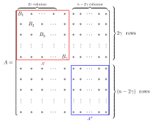
Figure 1: The matrix $A$ after permuting the rows an columns. $*$ denotes unspecified entries.

Since $(i_{p},j_{p})$ is a $Y$-special position, $(k_{p},\ell_{p})$ is a $Z$-special position we have $X_{\varphi}[i_{p},j_{p}]\in Y$, $X_{\varphi}[k_{p},\ell_{p}]\in Z$. Also $X_{\varphi}[i_{p},\ell_{p}]\in\{0,1\}$ and $X_{\varphi}[k_{p},j_{p}]\in\{0,1\}$. Further, $\operatorname{rank}(M_{{{\sf perm}}(B_{p})})=2$ if and only if $X_{\varphi}[k_{p},j_{p}]=X_{\varphi}[i_{p},\ell_{p}]=1$. Consider the following events: $F_{1}$: $\gamma\geq m/12$;   and $F_{2}$: Rows $i_{1},\ldots,i_{\gamma},k_{1}\ldots,k_{\gamma}$ are $1$-good.

Lemma 23.

Let ${A}$ and $A^{\prime\prime}$ be matrices as above. Then $\Pr_{\varphi}[perm({A^{\prime\prime}})\neq 0~{}|~{}F_{1},F_{2}]\geq 1-\frac{1}{n^{2}}.$

Proof.

Permanent of any matrix $M$ with entries from $Y\cup Z\cup\{0,1\}$ is zero if and only if $M$ has an all zero $s\times t$ sub matrix such that $s+t=n+1$.(See Theorem 12.1 in [22].) We begin with a bound on the probability that there is at least one column/row with all zero entries. Note that the event $F_{1}$ depends only on the entries of $X_{\varphi}$ being in $Y\cup Z$, and the event $F_{2}$ is independent of the rows and columns of $A^{\prime\prime}$. Thus, for any position $(i,j)$ in $A^{\prime\prime}$, we have $\Pr[\varphi(x_{i,j})=1]=\kappa n/N(1-2m/N)\approx\kappa n/N$, for large enough $n$. Thus,

$$\Pr[\forall j\in[n],\varphi(x_{ij})=0] \leq\left(1-\frac{\kappa n}{N}\right)^{n-2\gamma}\mbox{ and hence, }$$

$$\Pr[\exists i~{}\forall j\in[n],\varphi(x_{ij})=0] \leq n\cdot\left(1-\frac{\kappa n}{N}\right)^{n-2\gamma}~{}~{}\mbox{ by union bound}$$

Since $$\gamma=\mathcal{O}(m)=o(n) N=n^{2}$$ and ,

$$\Pr[\exists i~{}\forall j\in[n],\varphi(x_{ij})=0] \leq n\frac{\left(1-\frac{\kappa}{n}\right)^{n}}{\left(1-\frac{\kappa}{n}\right)^{2\gamma}}$$

As $n\rightarrow\infty$, the denominator $\left(1-\frac{\kappa}{n}\right)^{2\gamma}\rightarrow 1$. Now, consider $1<c<n^{\prime}-1$, where $n^{\prime}=n-2\gamma$. We estimate the probability that there exists an $c\times(n^{\prime}-c+1)$ all zero sub-matrix of $A^{\prime\prime}$. For any $c\times(n^{\prime}-c+1)$ sub-matrix $M$ of $A^{\prime\prime}$, $\Pr[M=0]=(1-\kappa/n)^{c(n^{\prime}-c+1)}$.

As there are ${n^{\prime}\choose c}^{2}$ many such sub-matrices $M$ of $A^{\prime\prime}$, we get

$$\Pr[\exists M,M=0] \leq{n^{\prime}\choose c}^{2}(1-\kappa/n)^{c(n^{\prime}-c+1)}$$

$$\leq(n^{\prime}e/c)^{c}(1-\kappa/n)^{c(n^{\prime}-c+1)}\approx e^{2c\log((n+1)/c)-\kappa c(n^{\prime}-c+1)/n}\leq e^{-4\log n}$$

the last inequality follows since, $\kappa=20\log n$, and hence $2c\log(n+1/c)-\kappa(c-1)(n^{\prime}-c+1)/n\leq-2$ for large enough $n$.

$$\Pr[perm(\mathcal{A^{\prime\prime}})=0\mid F_{1},F_{2}] \leq n\cdot\left(1-\frac{\kappa}{n}\right)^{n}+ne^{-4\log n}\leq n\left[\left(1-\frac{\kappa}{n}\right)^{n/\kappa}\right]^{\kappa}+1/n^{3}\leq n\cdot\mathrm{e}^{-\kappa}\leq 1/n^{2}.$$

The penultimate inequality in the above is obtained by substituting $\kappa=20\log n$. ∎

Let $F_{3}$ denote the event “${{\sf perm}}(A^{\prime\prime})\neq 0$”. Define sets of matrices:

$$\mathcal{A} \stackrel{{\scriptstyle\triangle}}{{=}}\left\{X_{\varphi}\mid\parbox{122.85876pt}{ $X_{\varphi}\in F_{1}\cap F_{2}\cap F_{3}$ and $\exists i\leq\gamma,\operatorname{rank}(M_{{{\sf perm}}(B_{i})})=1$ }\right\}; \mathcal{B}\stackrel{{\scriptstyle\triangle}}{{=}}\left\{X_{\varphi}\mid\parbox{122.85876pt}{ $X_{\varphi}\in F_{1}\cap F_{2}\cap F_{3}$ and $\forall i\leq\gamma,\operatorname{rank}(M_{{{\sf perm}}(B_{i})})=2$. }\right\}$$

Observation 5.

$\forall A\in\mathcal{A}$, $\operatorname{rank}({{\sf perm}}(A^{\prime}))<2^{\gamma}$ and $\forall B\in\mathcal{B},\operatorname{rank}({{\sf perm}}(B))\geq 2^{\gamma}$.

Lemma 24.

Let $\mathcal{A}$ and $\mathcal{B}$ as defined above. Then (a) $\Pr\limits_{\varphi\sim\mathcal{D}}[\operatorname{rank}(M_{{{\sf perm}}(X_{\varphi})})\geq 2^{\gamma})]\geq{\cal D}({\cal B})$; and (b) ${\cal D}(B)\geq{\cal D}({\cal A})$, where ${\mathcal{D}}(S)=\Pr\limits_{\varphi\sim\mathcal{D}}[X_{\varphi}\in S]$ for $S\in\{\mathcal{A},\mathcal{B}\}$.

Proof.

(a) follows from Observation 5. For (b), we establish a one-one mapping $\pi:\mathcal{A}\to\mathcal{B}$ defined as follows. Let $\varphi$ be such that $X_{\varphi}\in\mathcal{A}$. Consider $1\leq p\leq\gamma$ such that $\operatorname{rank}(M_{{{\sf perm}}(B_{p})})=1$. Then either $X_{\varphi}[k_{p},j_{p}]=0$ or $X_{\varphi}[i_{p},\ell_{p}]=0$ or both. If $X_{\varphi}[k_{p},j_{p}]=0$, then set $X_{\varphi^{\prime}}[k_{p},j_{p}]=1$, and $X_{\varphi^{\prime}}[k_{p},\iota_{p}]=0$ where $\iota_{p}\in[n]\setminus\{j_{1}\ldots,j_{\gamma},\ell_{1}\ldots,\ell_{\gamma}\}$ is the first index from left such that $X_{\varphi}[k_{p},\iota_{p}]=1$. Similarly, if $X_{\varphi}[i_{p},\ell_{p}]=0$, then set $X_{\varphi^{\prime}}[i_{p},\ell_{p}]=1$, and $X_{\varphi^{\prime}}[i_{p},\lambda_{p}]=0$ where $\lambda_{p}\in[n]\setminus\{j_{1}\ldots,j_{\gamma},\ell_{1}\ldots,\ell_{\gamma}\}$ is the first index from left such that $X_{\varphi}[k_{p},\lambda_{p}]=1$. Let $\varphi^{\prime}$ be the partition obtained from $\varphi$ by applying the above mentioned swap operation for every $1\leq p\leq\gamma$ with $\operatorname{rank}(M_{{{\sf perm}}(B_{p})})=1$, keeping other values of $\varphi$ untouched. Clearly $X_{\varphi^{\prime}}\in\mathcal{B}$. Set $\pi(X_{\varphi})\mapsto X_{\varphi^{\prime}}$. It can be seen that $\pi$ is an one-one map. Further, for any fixed $A\in\mathcal{A}$, $\Pr_{\varphi}[X_{\varphi}=A]=\Pr_{\varphi}[X_{\varphi}=\pi(A)]$ since $\varphi$ is independently and identically distributed for any position in the matrix. Thus we have $\mathcal{D}(\mathcal{A})\leq\mathcal{D}(\mathcal{B})$. ∎

Proof of Theorem 6.

It is enough to argue that $\Pr_{\varphi\sim\mathcal{D}}[X\varphi\in\mathcal{A}\cup\mathcal{B}]=1-O(\frac{1}{n^{2}})$, as $\mathcal{A}\cap\mathcal{B}=\emptyset$ . Now, $\Pr_{\varphi\sim\mathcal{D}}[X_{\varphi}\in\mathcal{A}\cup\mathcal{B}]=\Pr_{\varphi\sim\mathcal{D}}[F_{1}\cap F_{2}\cap F_{3}]$. By Lemma 19, $Pr_{\varphi\sim\mathcal{D}}[F_{1}]=1-2^{-\Omega(m)}$, by Lemma 4 combined with union bound we have $Pr_{\varphi\sim\mathcal{D}}[F_{2}]\geq 1-\gamma/n^{3}$ and by Lemma 23 $Pr_{\varphi\sim\mathcal{D}}[F_{3}|F_{1},F_{2}]\geq 1-2/n^{2}$. Thus we conclude $\Pr_{\varphi\sim\mathcal{D}}[F_{1}\cap F_{2}\cap F_{3}]=1-O(\frac{1}{n^{2}})$. As $\mathcal{D}(\mathcal{B}\cap\mathcal{A})=\mathcal{D}(\mathcal{A})+\mathcal{D}(\mathcal{B})$, by Lemma 24 we have $\Pr_{\varphi\sim\mathcal{D}}[\operatorname{rank}(M_{{{\sf perm}}(X_{\varphi})})\geq 2^{\gamma}]\geq 1/2(1-O(\frac{1}{n^{2}}))$. ∎

4.3 Putting them all together

Proof of Theorem 1

Proof.

Suppose $p_{lin}=\sum_{i=1}^{s}\prod_{j=1}^{t}f_{i,j}$ where $f_{i,j}$ are syntactically multi-linear $\Sigma\Pi\Sigma$ formula, with $s<2^{N^{1/4}}$, Let $f_{i,j}=\sum_{k=1}^{s^{\prime}}T_{i,j,k}$, and $T_{i,j,k}$ are products of variable disjoint linear forms, and hence ${\sf ROP}$s. Further, since the bottom fan-in of each $f_{i,j}$ is bounded by $N^{1/2+\lambda}$, we have $s_{T_{i,j,k}}\leq 2^{N^{1/2+\lambda}}$. Then by Lemma 17 and union bound there is an $i,j,k$ such that $\operatorname{rank}(M_{T_{i,j,k}^{\varphi}})\geq 2^{N^{4/15}}$ with probability at most $sts^{\prime}2^{-\Omega(m)}$. By Lemma 3 and 4, we have $\operatorname{maxrank}(\widehat{M}_{p_{lin}^{\varphi}})\leq 2^{N^{4/15}}$ with probability $1-o(1)$. However by Lemma 18, $\operatorname{maxrank}(\widehat{M}_{p_{lin}^{\varphi}})=\operatorname{rank}(M_{p_{lin}^{\varphi}})=2^{\Omega(m)}$ with probability at least $1-2^{-\Omega(m)}$, a contradiction. Hence $ss^{\prime}=2^{\Omega(N^{1/4})}$. ∎

Proof of Theorem 2

Proof.

Suppose $s<2^{N^{1/4}}$. Then by Lemma 17, the probability that there is an $f_{i,j}$ with $\operatorname{rank}(M_{f_{i,j}^{\varphi}})\geq 2^{N^{4/15}}$ is at most $2^{-\Omega(m)}s\cdot t=o(1)$. By Lemma 3 and 4, we have $\operatorname{maxrank}(\widehat{M}_{p_{lin}^{\varphi}})\leq 2^{N^{4/15}}$ with probability $1-o(1)$. However by Lemma 18, $\operatorname{maxrank}(\widehat{M}_{p_{lin}^{\varphi}})=\operatorname{rank}(M_{p_{lin}^{\varphi}})=2^{\Omega(m)}$ with probability $1-2^{-\Omega(m)}$, a contradiction. Hence $s\geq 2^{N^{1/4}}$. ∎

Proof of Theorem 3

Proof.

Suppose $s<2^{N^{1/4}}$. Then by Lemma 17, Probability that there is an $f_{i,j}$ with $\operatorname{rank}(M_{f_{i,j}^{\varphi}})\geq 2^{N^{4/15}}$ is at most $2^{-\Omega(m)}s\cdot t=o(1)$. By Lemma 3 and 4, we have $\operatorname{maxrank}(\widehat{M}_{{\sf perm}_{n}^{\varphi}})\leq 2^{N^{4/15}}$ with probability $1-o(1)$. However, by Theorem 6, $\operatorname{maxrank}(\widehat{M}_{{\sf perm}_{n}^{\varphi}})=\operatorname{rank}({\sf perm}_{n}^{\varphi})=2^{\Omega(m)}$ with probability $(1-1/n^{2})/2$, a contradiction. Hence $s\geq 2^{N^{1/4}}$. ∎

References

- [1] Manindra Agrawal and V. Vinay. Arithmetic circuits: A chasm at depth four. In FOCS, pages 67–75, 2008.
- [2] Devdatt Dubhashi and Alessandro Panconesi. Concentration of Measure for the Analysis of Randomized Algorithms. Cambridge University Press, New York, NY, USA, 1st edition, 2009.
- [3] Dima Grigoriev and Marek Karpinski. An exponential lower bound for depth 3 arithmetic circuits. In STOC, pages 577–582, 1998.
- [4] Ankit Gupta, Pritish Kamath, Neeraj Kayal, and Ramprasad Saptharishi. Arithmetic circuits: A chasm at depth three. In FOCS, pages 578–587, 2013.
- [5] Ankit Gupta, Pritish Kamath, Neeraj Kayal, and Ramprasad Saptharishi. Approaching the chasm at depth four. J. ACM, 61(6):33:1–33:16, 2014.
- [6] Neeraj Kayal. An exponential lower bound for the sum of powers of bounded degree polynomials. Electronic Colloquium on Computational Complexity (ECCC), 19:81, 2012.
- [7] Neeraj Kayal, Nutan Limaye, Chandan Saha, and Srikanth Srinivasan. STOC. pages 119–127, 2014.
- [8] Neeraj Kayal and Chandan Saha. Multi-k-ic depth three circuit lower bound. In STACS, pages 527–539, 2015.
- [9] Pascal Koiran. Arithmetic circuits: The chasm at depth four gets wider. Theor. Comput. Sci., 448:56–65, 2012.
- [10] Mrinal Kumar, Gaurav Maheshwari, and Jayalal Sarma. Arithmetic circuit lower bounds via maxrank. In Automata, Languages, and Programming - 40th International Colloquium, ICALP 2013, Riga, Latvia, July 8-12, 2013, Proceedings, Part I, pages 661–672, 2013.
- [11] Mrinal Kumar and Shubhangi Saraf. On the power of homogeneous depth 4 arithmetic circuits. In FOCS, pages 364–373, 2014.
- [12] Meena Mahajan, B. V. Raghavendra Rao, and Karteek Sreenivasaiah. Building above read-once polynomials: Identity testing and hardness of representation. In COCOON, pages 1–12, 2014.
- [13] Thierry Mignon and Nicolas Ressayre. A quadratic bound for the determinant and permanent problem. International Mathematics Research Notices, 2004(79):4241–4253, 2004.
- [14] Ran Raz. Multi-linear formulas for permanent and determinant are of super-polynomial size. In Proceedings of the 36th Annual ACM Symposium on Theory of Computing, Chicago, IL, USA, June 13-16, 2004, pages 633–641, 2004.
- [15] Ran Raz. Multilinear-nc neq multilinear-nc. In FOCS, pages 344–351, 2004.
- [16] Ran Raz. Multi-linear formulas for permanent and determinant are of super-polynomial size. J. ACM, 56(2), 2009.
- [17] Ran Raz and Amir Yehudayoff. Balancing syntactically multilinear arithmetic circuits. Computational Complexity, 17(4):515–535, 2008.
- [18] Ran Raz and Amir Yehudayoff. Lower bounds and separations for constant depth multilinear circuits. Computational Complexity, 18(2):171–207, 2009.
- [19] Amir Shpilka and Ilya Volkovich. Read-once polynomial identity testing. In STOC, pages 507–516, 2008.
- [20] Sébastien Tavenas. Improved bounds for reduction to depth 4 and depth 3. In MFCS, pages 813–824, 2013.
- [21] Leslie G. Valiant. Completeness classes in algebra. In STOC, pages 249–261, 1979.
- [22] J. H. van Lint and R. M. Wilson. A Course In Combinatorics. Cambridge University Press, 2nd edition, 2001.