Non-divisibility vs backflow of information in understanding revivals of quantum correlations for continuous-variable systems interacting with fluctuating environments

Abstract

We address the dynamics of quantum correlations for a bipartite continuous-variable quantum system interacting with its fluctuating environment. In particular, we consider two independent quantum oscillators initially prepared in a Gaussian state, e.g. a squeezed thermal state, and compare the dynamics resulting from local noise, i.e. oscillators coupled to two independent external fields, to that originating from common noise, i.e. oscillators interacting with a single common field. We prove non-Markovianity (non-divisibility) of the dynamics in both regimes and analyze the connections between non-divisibility, backflow of information and revivals of quantum correlations. Our main results may be summarized as follows: (i) revivals of quantumness are present in both scenarios, however, the interaction with a common environment better preserves the quantum features of the system; (ii) the dynamics is always non-divisible but revivals of quantum correlations are present only when backflow of information is present as well. We conclude that non-divisibility in its own is not a resource to preserve quantum correlations in our system, i.e. it is not sufficient to observe recoherence phenomena. Rather, it represents a necessary prerequisite to obtain backflow of information, which is the true ingredient to obtain revivals of quantumness.

I Introduction

Decoherence is a distinctive sign of the detrimental influence of the environment on a quantum system. In quantum information and technology, decoherence is the main obstacle to reliable quantum processing of information. More generally, decoherence is a widely accepted explanation for the loss of nonclassicality of quantum systems and for their transition to the classical realm zur01 ; paz01 . In the recent years, it has been recognized that the action of an environment on a system may also have some non-detrimental effects, at least for a transient. Indeed, non-trivial spectral structures and memory effects, usually leading to non-Markovian dynamics for the quantum system liu02 ; smi01 ; pii04 ; smi02 , may induce recoherence and revivals of quantum features.

The environment of a quantum system is usually made of several (classical and quantum) units with an overall complex structure. As a consequence, a full quantum treatment of the interaction betweeen a system and its environment is often challenging, or even unfeasible in a closed form. On the other hand, it is often the case that the overall action of the environment may be conveniently described as an external random force acting on the system, i.e. a classical stochastic field (CSF) gar01 . In general, one might expect that the modeling of a quantum environment as classical one leads to an incomplete description, i.e. such a description cannot capture the full quantum features of the dynamics. On the contrary, it has been proved that several system-environment interactions have a classical equivalent description hel01 ; hel02 ; cro01 ; wit01 ; str02 ; sto01 . In addition, there are experimental situations in which quantum systems interact with an inherently classical Gaussian noise ast01 ; gal01 ; abe01 ; str01 , or where the environment can be effectively simulated classically tur01 .

In this framework, the first goal of this paper is to analyze in details the dynamics of a bipartite system made of two independent quantum harmonic oscillators interacting with its classical fluctuating environments. In particular, we compare the dynamics of correlations in two different environmental situations. On the one hand, we consider a local noise model, where each oscillator interacts with its own classical environment. On the other hand, we also consider the situation where both the oscillators interact with a common environment, described by a single stochastic field. A similar analysis has been performed for qubit systems bel02 ; maz02 revealing a rich phenomenology.

Our work is also aimed at better analyzing the connections between the dynamics of quantumness, e.g. revivals of quantum correlations and the quantum-to-classical transition, and the non-Markovian features of the dynamics. In particular, we want to investigate the role of non-Markovianity itself (i.e. non-divisibility of the quantum dynamical map) against the role of the backflow of information, which is a sufficient (but not necessary) condition to prove non-Markovianity and, in turn, often used to witness its presence.

In order to introduce the subject, we remind that directly proving rhp ; ill01 ; ade01 the non-Markovian character of a dynamics is not always possible, as in many situations the full analytic form of the time-dependent quantum dynamical map is missing. When the direct verification is not possible, one may exploit witnesses of non-Markovianity, i.e. quantities that vanish in case of a Markovian dynamics. Even though the witnesses may successfully capture the memory feature of a non-Markovian process in many situations, they possess different physical meaning and may be ineffective in some specific situation. As an example, the BLP measure pii01 , and its continuous variable analogue based on fidelity nmc11 , have both a clear physical interpretation in terms of information flow from the environment back to the system. Used as a witness, the BLP measure has been proved useful and effective to quantify memory effects in several situations but it may also fail to detect non-Markovianity hai01 ; pii02 . On the other hand, recent results hp1 suggest that information backflow is the essential element in addressing non-Markovian dynamics of a quantum system and for this reason the BLP measure has been proposed as the definition of quantum non-Markovianity itself.

In this context, more information may be often extracted from the study of the quantum correlations of the system, e.g. the entanglement or the quantum discord. In fact, revivals of quantum features, especially in non-interacting bipartite systems, may be a signature of a non-Markovianity. This is what happens, e.g., for non-interacting qubits bel01 ; bel02 . On the other hand, the connection between revivals of correlations and backflow of information appears quite natural, especially in open quantum systems: a temporary and partial restoration of quantum coherence, previously lost during the interaction, is a sign of a memory effect, possibly of the environment, which is supposed to be storing correlations and sending them back to the system. Remarkably, revivals of correlations may also be found when the quantum system is interacting with a classical environment, suggesting that these feature reflects a property of the map, rather than a property of the environment. For qubit systems revivals have been detected in presence of Gaussian noise ben01 , and may even be found in the case of non-interacting qubits rlf01 . For a single oscillator, classical memory effects have been found to increase the survival time of quantum coherence catstf and, in particular, it has been proved that a detuning between the natural frequency of the system and the central frequency of the classical field induces revivals of quantum coherence.

For the system under investigation in this paper, non-Markovianity needs not to be witnessed, as it can be easily proven in a direct way. The stochastic description of the environment, in fact, allows us to determine the analytic form of the quantum dynamical map and to check straightforwardly its non-divisibility. On the other hand, information backflow may be revealed using fidelity witness nmc11 . Our results indicate that the dynamics is not divisible for both local and common noise, and that also revivals of quantumness appears in both cases, with the common case better preserving the quantum features of the system. At the same time, we found that revivals of quantum correlations are present only when non-Markovianity is present together with a backflow of information. We conclude that non-Markovianity itself is not the resource needed to preserve quantum correlations in our system. In other words, non-Markovianity alone is not a sufficient condition to induce revivals. Rather, it represents a necessary prerequisite to obtain backflow of information, which is the true ingredients to obtain revivals of quantumness.

The paper is organized as follows. In Sec.II we introduce the system and the stochastic modeling of both the environmental scenarios. In Sec. III we introduce the quantifiers of correlations and describe the initial preparation of the system, focusing on its inital correlations. In Sec. IV we analyze the dynamics of the correlations, delimiting the boundaries for the existence of revivals. In Sec. V we prove the nonmarkovianity of the dynamics and study the fidelity witness. Sec. VI summarizes the paper.

II The Interaction Model

We consider two non-interacting harmonic quantum oscillators with natural frequencies $\omega_{1}$ and $\omega_{2}$ and analyze the dynamics of this system in two different regimes: in the first one each oscillator is coupled to one of two independent non-interacting stochastic fields, we dub this scenario as the local noise case. In the second regime, the oscillators are coupled to the same classical stochastic field, so we dub this case as common noise. In both case, the Hamiltonian $H$ is composed by a free and an interaction term. The free Hamiltonian $H_{0}$ is given by

$$H_{0} =\hbar\sum_{j=1}^{2}\omega_{j}a_{j}^{\dagger}a_{j}$$ (1)

Unlike the free Hamiltonian $H_{0}$, which is the same in the description of both models, the interaction term $H_{I}$ differs. In the following subsections, we introduce the local and the common interaction Hamiltonian.

II.1 Local Interaction

The interaction Hamiltonian $H_{\hbox{\tiny L}\,}$ in the local model reads

$$H_{\hbox{\tiny L}\,}(t) =\sum_{j=1}^{2}a_{j}\bar{C_{j}}(t)e^{i\delta_{j}t}+a^{\dagger}_{j}C_{j}(t)e^{-i\delta_{j}t}$$ (2)

where the annihilation operators $a_{1},a_{2}$ represent the oscillators, each coupled to a different local stochastic field $C_{j}(t)$ with $j=1,2$, and $\delta_{j}=\omega_{j}-\omega$ is the detuning between the carrier frequency of the field and the natural frequency of the $j$-th oscillator. In the last equation and throughout the paper, we will consider the Hamiltonian rescaled in units of a reference level of energy $\hbar\omega_{0}$ (for a reason to be pointed out later). Under this condition, the stochastic fields $C_{1}(t),C_{2}(t)$, their central frequency $\omega$, the interaction time $t$, and the detunings all become dimensionless quantities.

The presence of fluctuating stochastic fields leads to an explicitly time-dependent Hamiltonian, whose corresponding evolution operator is given by

$$U(t)={\cal T}\exp\left\{-i\int_{0}^{t}\!\!ds\,H_{\hbox{\tiny L}\,}(s)\right\}\,,$$ (3)

where ${\cal T}$ is the time ordering. However, as the interaction Hamiltonian is linear in the annihiliation and creation operators of the two oscillators, the two-time commutator $[H_{\hbox{\tiny L}\,}(t_{1}),H_{\hbox{\tiny L}\,}(t_{2})]$ is always proportional to the identity. In particular, when the stochastic fields satisfy the conditions $C_{j}(t_{1})\bar{C_{j}}(t_{2})=C_{j}(t_{2})\bar{C_{j}}(t_{1})$, with $j=1,2$, the two-time commutator becomes

$$[H_{\hbox{\tiny L}\,}(t_{1}),H_{\hbox{\tiny L}\,}(t_{2})]= \sum_{j=1,2}2i\,\bar{C_{j}}(t_{1})C_{j}(t_{2})$$

$$\times\sin\left[\delta_{j}(t_{1}-t_{2})\right]\,\mathbb{I}_{12}$$ (4)

This form of the two-time commutator allows us to use the Magnus expansion mag1 ; mag2 to simplify the expression of the evolution operator (3) into

$$U(t)=\exp\left(\Xi_{1}+\Xi_{2}\right)$$ (5)

where the most general form of $\Xi_{1}$ and $\Xi_{2}$ is given by

$$\Xi_{1} =-i\int_{0}^{t}\!\!ds_{1}\,H_{I}(s_{1}),$$ (6)

$$\Xi_{2} =\frac{1}{2}\int_{0}^{t}\!ds_{1}\!\int_{0}^{s_{1}}\!\!ds_{2}\,\,[H_{I}(s_{1}),H_{I}(s_{2})].$$ (7)

The specific form of $\Xi_{1}$ for the local ($\Xi_{1}^{\hbox{\tiny L}\,}$) scenario is given by

$$\Xi_{1}^{\hbox{\tiny L}\,} =\sum_{j=1}^{2}\left(a_{j}^{\dagger}\phi_{j}(t)-a_{j}\phi_{j}^{*}(t)\right)$$ (8)

where

$$\phi_{j}(t) =-i\int_{0}^{t}ds\,e^{-i\delta_{j}s}C_{j}(s)\quad\mbox{with }j=1,2.$$ (9)

The evolution of the density operator of the system then reads

$$\rho_{L}(t) =\left[e^{\Xi^{\hbox{\tiny L}\,}_{1}}\rho(0)e^{(\Xi_{1}^{\hbox{\tiny L}\,})^{*}}\right]_{F}$$

$$=\left[D(\phi_{a},\phi_{b})\rho_{0}D^{\dagger}(\phi_{a},\phi_{b})\right]_{F}$$ (10)

where $D_{j}(\alpha)=\exp(\alpha a_{j}^{\dagger}-\alpha^{*}a_{j})$ is the displacement operator, $D(\alpha_{1},\alpha_{2})=D(\boldsymbol{\alpha})=D_{1}(\alpha_{1})D_{2}(\alpha_{2})$ and $\left[\ldots\right]_{F}$ is the average over the realizations of the stochastic fields.

In the local scenario, we assume each CSF

$$C_{j}(t)=C_{j}^{(x)}(t)+iC_{j}^{(y)}(t),$$

described as a Gaussian stochastic process with zero mean $[C_{j}^{(x)}(t)]_{F}=[C_{j}^{(y)}(t)]_{F}=0$ and autocorrelation matrix given by

$$\left[C_{j}^{(x)}(t_{1})C_{k}^{(x)}(t_{2})\right]_{F} =\left[C_{j}^{(y)}(t_{1})C_{k}^{(y)}(t_{2})\right]_{F}$$

$$=\delta_{jk}K(t_{1},t_{2})$$ (11)

$$\left[C_{j}^{(x)}(t_{1})C_{k}^{(y)}(t_{2})\right]_{F} =\left[C_{j}^{(y)}(t_{1})C_{k}^{(x)}(t_{2})\right]_{F}=0$$ (12)

where we introduced the kernel autocorrelation function $K(t_{1},t_{2})$. By means of the Glauber decomposition of the initial state $\rho(0)$

$$\rho(0)=\int\frac{d^{4}\boldsymbol{\zeta}}{\pi^{2}}\chi[\rho(0)](\boldsymbol{\zeta})D^{\dagger}(\boldsymbol{\zeta})$$ (13)

where $\chi[\rho](\boldsymbol{\zeta})=\mbox{Tr}[\rho D(\boldsymbol{\zeta})]$ is the symmetrically ordered characteristic function, the density matrix of the evolved state reads

$$\rho_{\hbox{\tiny L}\,}(t)=\mathcal{G}_{\hbox{\tiny L}\,}[\rho(0)]=\int\frac{d^{4}\boldsymbol{\zeta}}{\pi^{2}}g_{\hbox{\tiny L}\,}(\boldsymbol{\zeta})D(\boldsymbol{\zeta})\rho(0)D^{\dagger}(\boldsymbol{\zeta})$$ (14)

where we use the Gaussian function

$$g_{\hbox{\tiny L}\,}(\boldsymbol{\zeta})=\frac{\exp(-\frac{1}{2}\,\boldsymbol{\zeta}\cdot\boldsymbol{\Omega}\cdot\boldsymbol{\sigma}_{\hbox{\tiny L}\,}^{-1}\cdot\boldsymbol{\Omega}^{T}\cdot\boldsymbol{\zeta}^{T})}{\sqrt{\mbox{det}[\boldsymbol{\sigma}_{\hbox{\tiny L}\,}]}}$$ (15)

where $\boldsymbol{\sigma}_{\hbox{\tiny L}\,}$ and the symplectic matrix $\boldsymbol{\Omega}$ are given by

$$\boldsymbol{\Omega}=\left(\begin{array}[]{cc}0&1\vspace{0.1 cm}\\ -1&0\end{array}\right)\quad\boldsymbol{\sigma}_{\hbox{\tiny L}\,}=\left(\begin{array}[]{cc}\beta_{1}(t)\mathbb{I}_{2}&0\vspace{0.1 cm}\\ 0&\beta_{2}(t)\mathbb{I}_{2}\end{array}\right).$$ (16)

The matrix $\boldsymbol{\sigma}_{\hbox{\tiny L}\,}$ is the covariance of the noise function $g_{\hbox{\tiny L}\,}(\boldsymbol{\sigma})$ and its matrix elements are given by

$$\beta_{j}(t,t_{0})=\int_{t_{0}}^{t}\int_{t_{0}}^{t}ds_{1}ds_{2}\cos[\delta_{j}(s_{1}-s_{2})]K(s_{1},s_{2}).$$ (17)

II.2 Common Interaction

The Hamiltonian $H_{\hbox{\tiny C}\,}$ in the common interaction model reads

$$H_{\hbox{\tiny C}\,}(t) =\sum_{j=1}^{2}a_{j}e^{i\delta_{j}t}\bar{C}(t)+a^{\dagger}_{j}e^{-i\delta_{j}t}C(t)$$ (18)

where each oscillator, represented by the annihilation operators $a_{1},a_{2}$, is coupled to a common stochastic field $C(t)$ which is described as a Gaussian stochastic process with zero mean $[C^{(x)}]_{F}=[C^{(y)}]_{F}=0$ and the very same autocorrelation matrix of the local scenario.

Along the same lines of the local interaction model derivation, we use the Magnus expansion in order to get to the evolution operator. By asking the stochastic field to satisfy the relation $C(t_{1})\bar{C}(t_{2})=C(t_{2})\bar{C}(t_{1})$, the two-time commutator reads

$$[H_{\hbox{\tiny C}\,}(t_{1}),H_{\hbox{\tiny C}\,}(t_{2})] =\bar{C}(t_{1})C(t_{2})\sum_{j=1,2}2i\,\sin\left[\delta_{j}(t_{1}-t_{2})\right]\mathbb{I}_{12}.$$ (19)

The evolution operator for the common scenario is the same described in Eq. (5), where the specific form of $\Xi_{1}$ in the common interaction model is given by

$$\Xi_{1}^{\,\hbox{\tiny C}\,} =\sum_{j=1}^{2}\left(a_{j}^{\dagger}\psi_{j}(t)-a_{j}\psi_{j}^{*}(t)\right)$$ (20)

where

$$\psi_{j}(t) =-i\int_{0}^{t}ds\,e^{-i\delta_{j}s}C(s)\quad\mbox{with }j=1,2.$$ (21)

The evolution of the density operator of the system then reads

$$\rho(t)=\left[e^{\Xi^{\,\hbox{\tiny C}\,}_{1}}\rho(0)e^{(\Xi^{\,\hbox{\tiny C}\,}_{1})^{*}}\right]_{F}=\left[D(\psi_{1},\psi_{2})\rho_{0}D^{\dagger}(\psi_{1},\psi_{2})\right]_{F}$$ (22)

which, following the same steps of the derivation presented in the previous subsection, leads to

$$\rho_{\hbox{\tiny C}\,}(t)=\mathcal{G}_{\hbox{\tiny C}\,}[\rho(0)]=\int\frac{d^{4}\boldsymbol{\zeta}}{\pi^{2}}g_{\hbox{\tiny C}\,}(\boldsymbol{\zeta})D(\boldsymbol{\zeta})\rho(0)D^{\dagger}(\boldsymbol{\zeta})$$ (23)

where we use the Gaussian function

$$g_{\hbox{\tiny C}\,}(\boldsymbol{\zeta})=\frac{\exp(-\frac{1}{2}\,\boldsymbol{\zeta}\cdot\boldsymbol{\Omega}\cdot\boldsymbol{\sigma}_{\hbox{\tiny C}\,}^{-1}\cdot\boldsymbol{\Omega}^{T}\cdot\boldsymbol{\zeta}^{T})}{\sqrt{\mbox{det}[\boldsymbol{\sigma}_{\hbox{\tiny C}\,}]}}$$ (24)

$\boldsymbol{\sigma}_{\hbox{\tiny C}\,}$ being its covariance matrix, given by

$$\boldsymbol{\sigma}_{\hbox{\tiny C}\,}=\left(\begin{array}[]{cc}\beta_{1}(t)\mathbb{I}_{2}&\boldsymbol{R}\vspace{0.1 cm}\\ \boldsymbol{R}&\beta_{2}(t)\mathbb{I}_{2}\end{array}\right)$$ (27)

$$\boldsymbol{R}=\left(\begin{array}[]{cc}\beta_{\hbox{\tiny C}\,}(t)&\gamma_{\hbox{\tiny C}\,}(t)\vspace{0.1 cm}\\ \gamma_{\hbox{\tiny C}\,}(t)&\beta_{\hbox{\tiny C}\,}(t)\end{array}\right)$$ (30)

with the matrix elements given by

$$\beta_{c}(t,t_{0}) =\int_{t_{0}}^{t}\int_{t_{0}}^{t}ds_{1}ds_{2}\cos[(\delta_{1}s_{1}-\delta_{2}s_{2})]K(s_{1},s_{2}),$$

$$\gamma_{c}(t,t_{0}) =\int_{t_{0}}^{t}\int_{t_{0}}^{t}ds_{1}ds_{2}\sin[(\delta_{1}s_{1}-\delta_{2}s_{2})]K(s_{1},s_{2}).$$ (31)

II.3 Covariance Matrix dynamics in local and common interaction

The dynamical maps described by Eqs. (14) and (23) correspond to Gaussian channels, i.e. the evolution, in both regimes, preserves the Gaussian character of the input state. In turn, this is a useful features, since in this case quantum correlations, entanglement and discord, may be evaluated exactly. We also remind that Gaussian channels represent the short times solution of Markovian (dissipative) Master equations in the limit of high-temperature environment. In the following, this link will be exploited to analyze the limiting behaviour of the two-mode dynamics.

In order to get quantitative results, we assume that fluctuations in the environment are described by Ornstein-Uhlenbeck Gaussian processes, characterized by a Lorentzian spectrum and a kernel autocorrelation function

$$K(t_{1},t_{2})=\frac{1}{2}\lambda t_{\hbox{\tiny E}\,}^{-1}\exp({-|t_{1}-t_{2}|/t_{\hbox{\tiny E}\,}})\,,$$

where $\lambda$ is a coupling constant and $t_{\hbox{\tiny E}\,}$ is the correlation time of the environment. We also assume the case of resonant oscillators $(\omega_{1}=\omega_{2}=\omega_{0})$, which implies that the oscillators are identically detuned from the central frequency of the classical stochastic field, i.e.

$$\delta_{1}=\delta_{2}=\delta=1-\frac{\omega}{\omega_{0}}\,.$$

This assumptions simplifies the expression of the state dynamics: in the local scenario, leading to $\beta_{1}(t)=\beta_{2}(t)=\beta(t)$ and, in turn,

$$\rho_{\hbox{\tiny L}\,}(t) =\mathcal{E}_{\hbox{\tiny L}\,}[\rho(0)](t)=$$

$$=\int\frac{d^{4}\boldsymbol{\zeta}}{(\pi\beta(t))^{2}}\exp\left(-\frac{|\boldsymbol{\zeta}|^{2}}{\beta(t)}\right)D(\boldsymbol{\zeta})\rho(0)D^{\dagger}(\boldsymbol{\zeta})$$ (32)

where $\beta(\Delta t=t-t_{0})=\beta(t,t_{0})$ with the Ornstein-Uhlenbeck kernel is

$$\beta(t)= \frac{\lambda}{[1+(\delta\,t_{\hbox{\tiny E}\,})^{2}]^{2}}\Big{\{}t-t_{\hbox{\tiny E}\,}+(\delta\,t_{\hbox{\tiny E}\,})^{2}(t+t_{\hbox{\tiny E}\,})$$

$$+t_{\hbox{\tiny E}\,}\,e^{-t/t_{\hbox{\tiny E}\,}}\left[(1-(\delta\,t_{\hbox{\tiny E}\,})^{2})\cos\delta\,t-2\delta\,t_{\hbox{\tiny E}\,}\sin\delta\,t\right]\!\Big{\}}.$$ (33)

In the common noise case, the condition of resonant oscillators implies $\beta_{1}(t)=\beta_{2}(t)=\beta_{c}(t)=\beta(t)$ and $\gamma_{c}(t)=0$, leading to simplified matrices $\boldsymbol{R}$ and $\boldsymbol{\sigma}_{\hbox{\tiny C}\,}$ given by

$$\boldsymbol{R}=\left(\begin{array}[]{cc}\beta(t)&0\vspace{0.1 cm}\\ 0&\beta(t)\end{array}\right)\quad\boldsymbol{\sigma}_{\hbox{\tiny C}\,}=\left(\begin{array}[]{cc}\beta(t)\mathbb{I}_{2}&\boldsymbol{R}\vspace{0.1 cm}\\ \boldsymbol{R}&\beta(t)\mathbb{I}_{2}\end{array}\right)$$ (34)

corresponding to the Gaussian channel

$$\rho(t) =\mathcal{E}_{\hbox{\tiny C}\,}[\rho(0)](t)=$$

$$=\int\frac{d^{2}\zeta}{\pi\beta(t)}\exp\left(-\frac{|\zeta|^{2}}{\beta(t)}\right)D(\zeta,\zeta)\rho(0)D^{\dagger}(\zeta,\zeta).$$ (35)

As for the initial state $\rho(0)$ of the system, we assume a generic squeezed thermal state (STS), which is a zero-mean Gaussian state, described by a Gaussian characteristic function $\chi[\rho(0)](\boldsymbol{\zeta})=\exp\left(-\frac{1}{2}\boldsymbol{\zeta}^{T}\boldsymbol{\sigma}_{\!\hbox{\tiny STS}\,}\boldsymbol{\zeta}\right)$ where the covariance matrix $\boldsymbol{\sigma}_{\!\hbox{\tiny STS}\,}$ of the state has the general form

$$\boldsymbol{\sigma}_{\!\hbox{\tiny STS}\,}=\frac{1}{2}\left(\begin{array}[]{cc}A\,\mathbb{I}_{2}&C\sigma_{z}\\ C\sigma_{z}&B\,\mathbb{I}_{2}\end{array}\right),$$ (36)

where $\sigma_{z}=\mbox{diag}(1,-1)$ is the $z$ Pauli matrix. This covariance matrix corresponds to a density operator of the form

$$\rho=S_{2}(r)(\nu_{1}\otimes\nu_{2})S_{2}(r)^{\dagger}$$ (37)

where $S_{2}(r)=\exp\{r(a_{1}^{\dagger}a_{2}^{\dagger}-a_{1}a_{2})\}$ is the two-mode squeezing operator and $\nu_{j}$ is a single-mode thermal state

$$\nu_{j}=\frac{1}{\bar{n}_{j}}\sum_{m}\left(\frac{\bar{n}_{j}}{\bar{n}_{j}+1}\right)^{m}|m\rangle\langle m|.$$ (38)

The physical state depends on three real parameters: the squeezing parameter $r$ and the two numbers $\bar{n}_{1},\bar{n}_{2}$, which are related to the parameters $A,B,C$ of eq. (36) by the relations

$$A =\cosh(2r)+2\bar{n}_{1}\cosh^{2}r+2\bar{n}_{2}\sinh^{2}r$$

$$B =\cosh(2r)+2\bar{n}_{1}\sinh^{2}r+2\bar{n}_{2}\cosh^{2}r$$

$$C =(1+\bar{n}_{1}+\bar{n}_{2})\sinh(2r).$$ (39)

As the squeezed thermal state is a Gaussian state and the dynamics in both scenarios is described by a Gaussian channel, the output state at any time is Gaussian as well, so it is determined only by the covariance matrix. By evaluating the characteristic function of the evolved state, one finds that the covariance matrices of the state at time $t$ in the local and common scenarios are

$$\boldsymbol{\beta}_{\hbox{\tiny L}\,}(t) =\boldsymbol{\sigma}_{\!\hbox{\tiny STS}\,}+2\,\boldsymbol{\sigma}_{\hbox{\tiny L}\,}(t)$$ (40)

$$\boldsymbol{\beta}_{\hbox{\tiny C}\,}(t) =\boldsymbol{\sigma}_{\!\hbox{\tiny STS}\,}+2\,\boldsymbol{\sigma}_{\hbox{\tiny C}\,}(t)\,,$$ (41)

where $\boldsymbol{\sigma}_{\hbox{\tiny L}\,}(t)$ and $\boldsymbol{\sigma}_{\hbox{\tiny C}\,}(t)$ are given in Eqs. (16) and (34) respectively. As mentioned before, the Gaussian character of the states is preserved by the dynamics. Nevertheless, while the output state in the local scenario is always a STS, i.e. at any time it can be put in a diagonal form by means of a two-mode squeezing operation, the output state in the common scenario ceases to be an STS as soon as the interaction starts.

III Quantum Correlations

Systems possessing quantum features have proved themselves useful in many fields, e.g. quantum information, quantum computation and quantum estimation, increasing the performances of computation protocols and precision measurements. In the case of bipartite systems, the quantumness lies both in the nonclassicality of the state and in the correlations between the different parts of the system. In this section, we introduce two well-known markers of correlations, entanglement and quantum discord.

III.1 Entanglement

While classical multipartite systems, though being correlated, are always described in a quantum picture by separable states, quantum multipartite systems may show nonclassical correlations which require a description in terms of non-separable density operators. Aiming at quantifying these quantum correlations, the entanglement measures the degree of non-separability of a quantum system. For a bipartite Gaussian state $\rho$ with covariance matrix $\sigma$, the entanglement is given by the logarithmic negativity, which is defined as

$$\mathcal{N}(\rho)=\mbox{max}\{0,-\log(2\tilde{d}_{-})\}$$ (42)

where $\tilde{d}_{-}$ is the smallest symplectic eigenvalue of the partially transposed covariance matrix $\sigma^{\hbox{\tiny PT}\,}=\Delta\sigma\Delta$ with $\Delta=\mbox{diag}(1,-1,1,1)$. As stated by Simon sim1 , a two-mode gaussian state is separable if and only if the symplectic eigenvalue satisfies the relation $\tilde{d}_{-}\geq\frac{1}{2}$. Any violation of the latter implies that the state is non-separable (or entangled) and leads to a positive measure of the entanglement given in (42).

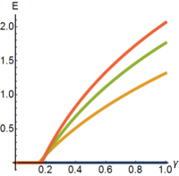
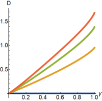
Figure 1: Quantum correlations of STS for different values of the energy $\epsilon$. Left panel: Entanglement of a STS as a function of squeezing parameter $\gamma$. The STS is entangled as long as $\gamma$ overtakes a threshold value that depends on the energy $\epsilon$. Right panel: Discord of a STS as a function of squeezing parameter $\gamma$. The STS is always a discordant state unless $\gamma=0$. In both panels, from bottom to top, $\epsilon=0$ (blue line), , $\epsilon=1$ (yellow line) , $\epsilon=2$ (green line) , $\epsilon=3$ (red line)

III.2 Quantum Discord

The total amount of the correlations possessed by a bipartite quantum state $\rho$ is called mutual information and is given by

$$\mathcal{I(\rho)}=S(\rho_{1})+S(\rho_{2})-S(\rho),$$ (43)

where $S(\rho_{j})$ is the Von Neumann entropy of the $j$-th subsystem. Usually, the mutual information can be divided into two parts: a classical part $\mathcal{C}(\rho)$ and a quantum part $\mathcal{D}(\rho)$, which takes name of quantum discord. The classical correlations, defined as the maximum amount of information extractable from one subsytem by performing local operations on the other, are given by

$$\mathcal{C}(\rho)=\mbox{max}_{\Pi_{i}}\Big{\{}S(\rho_{1})-\sum_{i}p_{i}S(\rho^{\Pi_{i}}_{1|2})\Big{\}}$$ (44)

where $\rho^{\Pi_{i}}_{1|2}=\mbox{Tr}_{2}(\rho\mathbb{I}\otimes\Pi_{i})$ is the state after the measurement on system 2 with probability $p_{i}=\mbox{Tr}_{1,2}(\rho\mathbb{I}\otimes\Pi_{i})$. The quantum discord is defined as the difference between the total correlations and the classical correlations:

$$\mathcal{D}(\rho)=\mathcal{I}(\rho)-\mathcal{C}(\rho).$$ (45)

The quantum discord then measures the amount of correlations whose origin cannot be addressed to the action of local operations or classical communication. However, computing the quantum discord may be challenging as it usually implies finding the POVM that maximizes the classical correlations. In the case of Gaussian states, the form of the POVM maximizing the classical correlations is known gio0 ; gio1 and the quantum discord depends only on the covariance matrix by the relation

$$\mathcal{D}(\rho)=h(\sqrt{I_{2}})-h(d_{-})-h(d_{+})+h\left(\sqrt{E_{min}}\right),$$ (46)

where $d_{-}$ and $d_{+}$ are the symplectic eigenvalues of the covariance matrix, $I_{1},I_{2},I_{3},I_{4}$ are the so-called symplectic invariants, $h(x)=(x+\frac{1}{2})\log(x+\frac{1}{2})-(x-\frac{1}{2})\log(x-\frac{1}{2})$ and gio1

$$E_{min}=\begin{cases}\left[\frac{2|I_{3}|+\sqrt{4I_{3}^{2}+(4I_{2}-1)(4I_{4}-1)}}{4I_{2}-1}\right]^{2}&\mbox{if }R_{\sigma}\leq 1\\ \frac{I_{1}I_{2}+I_{4}-I_{3}^{2}-\sqrt{(I_{1}I_{2}+I_{4}-I_{3}^{2})^{2}-4I_{1}I_{2}I_{4}}}{2I_{2}}&\mbox{if }R_{\sigma}>1\end{cases}$$ (47)

where

$$R_{\sigma}=\frac{4(I_{1}I_{2}-I_{4})^{2}}{(I_{1}+4I_{4})(1+4I_{2})I_{3}^{2}}\,.$$

For Gaussian states satisfying the second condition, the maximum amount of extractable information is achieved by measuring a canonical variable (e.g. by homodyne detection in optical systems hmqd ). On the other hand, for states falling in the first set, the optimal measurement is more general, and coincides with the projection over coherent states for STSs. For a generic Gaussian state, with covariance matrix $\sigma$ written in a block form

$$\sigma=\left(\begin{array}[]{cc}\mathbb{A}&\mathbb{C}\\ \mathbb{C}^{T}&\mathbb{B}\end{array}\right)$$ (48)

the symplectic invariants are $I_{1}=\mbox{det}\,\mathbb{A}$, $I_{2}=\mbox{det}\,\mathbb{B}$, $I_{3}=\mbox{det}\,\mathbb{C},I_{4}=\mbox{det}\,\sigma$.

III.3 STS correlations

In order to assess the dynamics of entanglement and discord in the presence of noise, we briefly review the static properties of quantum correlations bru15 for a squeezed thermal state. We consider the case of identical thermal states $(\bar{n}_{1}=\bar{n}_{2}=\bar{n})$ and use a convenient representation of STSs, built upon re-parametrizing the covariance matrix by means of its total energy $\epsilon=2(\bar{n}+n_{s}+2\bar{n}\,n_{s})$, with $n_{s}=\sinh^{2}r$, and a normalized squeezing parameter $\gamma\in[0,1]$, such that

$$n_{s} =\gamma\epsilon\quad\quad\bar{n}=\frac{(1-\gamma)\epsilon}{1+2\gamma\epsilon}.$$

Note that, for $\gamma=0$ the state has only thermal energy ($\epsilon=\bar{n}$) while for $\gamma=1$ the total amount of energy comes from the two-mode squeezing operation ($\epsilon=\sinh^{2}r$).

Fig.1 shows the quantum correlations of a STS as a function of the energy $\epsilon$ and the squeezing parameter $\gamma$. The left panel shows that the STS is entangled as long as $\gamma$ overtakes a threshold value which depends on the total amount of energy. Conversely, the quantum discord of a STS is always positive, unless the state is purely thermal, i.e. with zero squeezing. ($\gamma=0$). Notice that the states considered in this paper belongs to the class of Gaussian states for which the Gaussian discord equals the full quantum discord pir14 .

IV Dynamics of Quantum Correlations

Before proceeding with a detailed analysis of the dynamics of the quantum correlations, let us focus on the function $\beta(t)$, in order to understand which parameters affect the dynamics of the output state. As a matter of fact, the function $\beta(t)$, in (II.3) dependent on only two parameters (except time $t$), as it can be rescaled in units of $t_{\hbox{\tiny E}\,}$ by assuming $\tilde{\delta}=\delta t_{\hbox{\tiny E}\,}$, $\tilde{\lambda}=\lambda\,t_{\hbox{\tiny E}\,}$, $\tilde{t}=t/t_{\hbox{\tiny E}\,}$, leading to the expression (in which tildes have already been dropped)

$$\beta(t)= \,\frac{\lambda}{[1+\delta^{2}]^{2}}\Big{\{}t-1+\delta^{2}(t+1)$$

$$+\,e^{-t}\left[(1-\delta^{2})\cos\delta\,t-2\delta\,\sin\delta\,t\right]\!\Big{\}}.$$ (49)

Intuitively, given the form of the covariance matrices in Eqs. (40) and (41) one realizes that when $\beta(t)$ shows a monotonous behaviour, the system cannot gain any quantum features, or go back to the initial state at any value of the interaction time. Conversely, an oscillating $\beta(t)$ would let the system orbiting in the parameter space, which means that the quantum features of the output state may have a chance to be restored.

Formally, upon imposing the condition $d\beta(t)/dt=0$ leads to the following equation

$$2\lambda\,\frac{1-e^{-t}(\cos\delta t-\delta\sin\delta t)}{1+\delta^{2}}=0$$ (50)

which can not be analitically solved. The left panel of Fig. 2 contains a numerical plot of the solutions of (50) and shows the existence of a lower bound on the rescaled detuning $\delta$ for the oscillations of $\beta(t)$. The lower bound is represented by the black dashed line, corresponding to

$$\delta_{0}=\frac{3\pi}{2}[\mbox{\small{ProductLog}}(\frac{3\pi}{2})]^{-1}\simeq 3.644\,,$$

independently of $\lambda$.

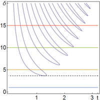
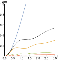
Figure 2: Left panel: Contourplot of $d\beta(t)/dt=0$ as a function of $t$ and $\delta$. The purple curve represents the solution of $d\beta(t)/dt=0$. The black dashed line represents the maximum value of $\delta=\delta_{0}$ for which $\beta(t)$ does not oscillate. Right panel: $\beta(t)$ for different values of $\delta$. From bottom to top, the other lines are for $\delta=1$ (blue), $\delta=5$ (yellow), $\delta=10$ (green), $\delta=15$ (red). An oscillating behavior is present only if $\delta>\delta_{0}$.

With this in mind, we now examinate the dynamics of quantum correlations of initially maximally entangled squeezed thermal states ($\gamma=1$) and two-mode thermal states ($\gamma=0)$ in presence of local and common stochastic environments. In order to be able of comparing the results of the different scenarios, we remind we already limited the analysis to resonant oscillators and that we assume identical the rescaled coupling constant $\lambda^{(c)}$ for the common scenario and $\lambda^{(1)},\lambda^{(2)}$ for the local scenario, $\lambda^{(c)}=\lambda^{(1)}=\lambda^{(2)}=\lambda$.

Let us start by addressing the dynamics of correlations of an initially entangled STS: the upper panels in Fig. 3 show how the classical stochastic fields, whether they be local or common, induce loss of correlations in time. However, the decay rate of correlations is not the same in both scenarios: indeed, the presence of a common stochastic field is less detrimental, i.e. the interaction with the same environment leads to a slower loss of correlations. In all the four panels, the green line corresponds to $\delta=\delta_{0}$, the threshold value over which $\beta(t)$ shows an oscillating behavior. As it is possible to see, $\delta=\delta_{0}$ plays the role of the threshold value also in the case of the correlations. In fact, detunings bigger than $\delta_{0}$ induce revivals of entanglement (upper right) and discord (lower left and right). The entanglement dynamics of the upper panel allows us to point out an important issue: $\delta>\delta_{0}$ is a necessary condition for an oscillating $\beta(t)$, though revivals of entanglement also depend on the rescaled coupling $\lambda$. In other words, when $\delta>\delta_{0}$, the symplectic eigenvalue $\tilde{d_{-}}$ of (42) flows in time in unison with $\beta(t)$, without necessarily violating the separability condition $\tilde{d_{-}}\geq\frac{1}{2}$. This explains the presence of a plateau in the entanglement of the common scenario with $\delta=\delta_{0}$.

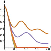
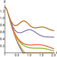
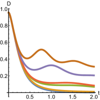
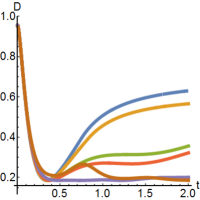
Figure 3: (Color Online) Dynamics of correlations in presence of CSFs for different values of rescaled detuning $\delta$. Upper left panel: Entanglement dynamics in local scenario as a function of time $t$. Upper right panel: Entanglement dynamics in common scenario as a function of time $t$. In both scenarios, the entanglement possessed by the system may revive. Lower left panel: Discord dynamics in local scenario as a function of time $t$. The initial discord decreases in time. Right left panel: Discord dynamics in common scenario as a function of time $t$. The initial discord decreases, reaches a minimum and the increases monotonically as a consequence of the interaction. In all panels, we set $\epsilon=1,\gamma=1,\lambda=1$, and, from bottom to top, $\delta=0$ (blue line), $\delta=2$ (yellow line), $\delta=\delta_{0}$ (green line), $\delta=4$ (red line), $\delta=6$ (purple line), $\delta=8$ (brown line).

Let us now focus on the discord dynamics (see the the lower panels in Fig. 3). While the entanglement shows a vanishing behavior in both scenarios in any setup of parameters, the same cannot be said for the quantum discord. While in the local scenario the initial discord tends to vanish, the common interaction introduces some correlations which clearly arise after the drop of the initial discord cic13 . The effect of the common stochastic field on the dynamics of the quantum discord is even clearer in the case of thermal input states (squeezing parameter $\gamma=0$). The upper left panel of Fig. 4 shows the discord evolution of the state $\rho=\nu_{1}\otimes\nu_{2}$ in the common scenario. The interaction transforms the initial zero-discord state into a discord state without affecting the separability of the input state (the symplectic eigenvalue $\tilde{d}_{-}$ always satisfies the condition $\tilde{d}_{-}\geq\frac{1}{2}$, as is apparent from the upper right panel of Fig. 4).

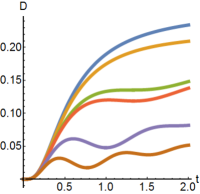
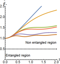
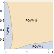
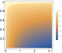
Figure 4: Upper panels: Correlations of a two-mode thermal state. Left panel: discord dynamics in time $t$ for different values of $\delta$. The initially zero-discord state becomes a discord state because of the interaction. Right panel: dynamics of symplectic eigenvalue $\tilde{d}_{-}$ for different values of $\delta$. The state always remains separable, though becoming a discord state. In both panels we have $\epsilon=1,\gamma=0,\lambda=1$ and, from top to bottom, $\delta=0$ (blue line), $\delta=2$ (yellow line), $\delta=\delta_{0}$ (green line), $\delta=4$ (red line), $\delta=6$ (purple line), $\delta=8$ (brown line). Lower left panel: Regionplot of the POVM minimizing the quantum discord. We set $\epsilon=1,\delta=3,\lambda=1$. Lower right panel: contourplot of the asymptotic value of the quantum discord as a function the input state parameters $\epsilon$ and $\gamma$. We set $\delta=3,\lambda=1$.

Furthermore, the quantum discord tends to an asymptotic value which depends on both the energy $\epsilon$ and the squeezing parameter $\gamma$ of the input Gaussian state, but it is not affected by the parameters of the environment $\lambda$ and $\delta$. Indeed, this can be seen as a consequence of the non-markovianity of the quantum map, as the long-time dynamics is influenced by the input state. A contourplot of the asymptotic value of the Discord as a function of $\epsilon$ and $\gamma$ is shown in the lower right panel of Fig. 4. Finally, we want to mention that the POVM that minimizes the quantum discord changes in time preserving the continuity of the discord itself. As an example, we report one particular scenario in the lower left panel of Fig. 4 where the regions corresponding to the two POVMs are coloured differently.

V Non Divisibility vs Information Backflow

The presence of revivals of correlations might be interpreted as a signature of some form of information backflow between the system and the environment, a phenomenon typically associated to non-Markovian effects. It is the purpose of this section to reveal the non-Markovian character of the Gaussian maps of both scenarios and explore the link between non-divisibility and information backflow, analyzing the evolution of the Fidelity of two input states.

A completely positive map $\mathcal{E}_{(t,t_{0})}$ describing the dynamical evolution of a quantum system is said to be divisible if it satisfies the decomposition rule $\mathcal{E}_{(t_{2},t_{0})}=\mathcal{E}_{(t_{2},t_{1})}\mathcal{E}_{(t_{1},t_{0})}$ for any $t_{2}\geq t_{1}\geq t_{0}$. Divisibility is often assumed to be the key concept to characterize non-Markovianity in the quantum regime and a completely positive map is said to be non-Markovian it it violates the decomposition rule for some set of times.

In our system, it is straightforward to prove that the Gaussian maps (14) and (23) do not satisfy the divisibility conditions, i.e. they cannot describe a Markovian dynamics. In order to prove this results, we notice that the composition of maps $\mathcal{E}_{\hbox{\tiny L}\,}(\Delta t_{2})\mathcal{E}_{\hbox{\tiny L}\,}(\Delta t_{1})$ corresponds to a convolution, leading to $\mathcal{E}_{\hbox{\tiny L}\,}(\Delta t_{2})\mathcal{E}_{\hbox{\tiny L}\,}(\Delta t_{1})=\mathcal{E}_{\hbox{\tiny L}\,}(\Delta t_{1}+\Delta t_{2})$. This condition is satisfied if and only if

$$\beta(\Delta t_{1}+\Delta t_{2})=\beta(\Delta t_{1})+\beta(\Delta t_{2}).$$ (51)

which is not satisfied for any choice of the parameters $\delta$ and $\lambda$, thus implying that the map is always non-Markovian. A similar proof can be obtained for the common noise map $\mathcal{E}_{\hbox{\tiny C}\,}(\Delta t)$.

We are now ready to discuss the connections between revivals of correlations, non-divisibility and information backflow. As we already mentioned in the introduction, non-Markovianity may be revealed by some witnesses, as the $BLP$ measure or the analogue measure based on fidelity for CV systems. Both techniques are based on the contractive property (valid for Markovian dynamics) of the trace distance and the Bures distance, respectively. Therefore, a non-monotonous behaviour of the trace distance or the fidelity is a signature of non-Markovianity. Furthermore, both these witnesses possess physical meaning: the trace distance is directly related to the probability of discriminating two states in time, whereas the Bures distance may be used to evaluate upper and lower bounds of the very same error probability defined by the trace distance. Therefore, a non-monotonous dynamics also implies a partial clawback of distinguishability of two input states, which has been interpreted as a sign of a backflow of informationpii03 . A measure of non-Markovianity $\mathcal{N}_{\mathcal{F}}$ can be constructed by the violation of the contractive property of the fidelity,

$$\mathcal{N}_{\mathcal{F}}=\frac{1}{2}\int\frac{1}{2}\int\left(\Big{|}\frac{d}{dt}D_{B}(\rho_{1},\rho_{2})\Big{|}+\frac{d}{dt}D_{B}(\rho_{1},\rho_{2})\right)dt,$$ (52)

where we used the Bures distance

$$D_{B}(\rho_{1},\rho_{2})=\sqrt{2\Big{[}1-\sqrt{\mathcal{F}(\rho_{1},\rho_{2})}\Big{]}}.$$ (53)

The quantity $\mathcal{N}_{\mathcal{F}}$ is nonzero only when the derivative of the Bures distance is positive, i.e. the contractive property is violated and the fidelity has a non-monotonous behaviour. In our system, the fidelity between any pair of two-mode Gaussian states

$$\mathcal{F}(\rho_{1},\rho_{2})=\Big{[}\mbox{Tr}\sqrt{\sqrt{\rho_{1}}\rho_{2}\sqrt{\rho_{1}}}\,\Big{]}.$$ (54)

may be evaluated analytically mar01 , though its expression is cumbersome and will not reported here.

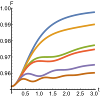
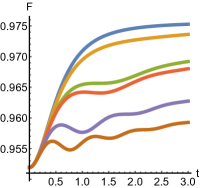
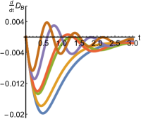
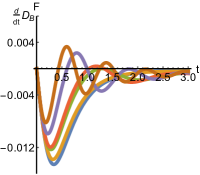
Figure 5: Dynamics of Fidelity and Bures distance derivative for different values of rescaled detuning $\delta$. Upper left panel: dynamics of Fidelity in a local scenario. Upper right panel: dynamics of Fidelity in a common scenario. In both situations, Fidelity ceases to oscillate when $\delta$ is lower than the threshold value $\delta_{0}$. The distinguishability of the input states diminishes monotonically in time and no backflow of information is detected. Lower left panel: derivative of Bures distance in local scenario. Lower right panel: derivative of Bures distance in common scenario. The curves with a positive part of derivative of Bures distance have $\delta>\delta_{0}$ and correspond to the curves in the upper panels where oscillations of Fidelity are shown. In all panels, we set $\epsilon_{1}=2,\epsilon_{2}=1,\gamma_{1}=\gamma_{2}=1,\lambda=1$ and, from top to bottom $\delta=0$ (blue line), $\delta=2$ (yellow line), $\delta=\delta_{0}$ (green line), $\delta=4$ (red line), $\delta=6$ (purple line), $\delta=8$ (brown line).

In Fig.5 we show the time evolution of the fidelity and the derivative of the Bures distance between a pair of two-mode squeezed vacuum states ($\gamma=1$) with different energies ($\epsilon_{1}\neq\epsilon_{2}$). The existence of sets of parameters leading to a non-monotonous behavior of the fidelity and a region of positive derivative of Bures distance is enough to confirm the already proven non-Markovianity of both maps. However, non-Markovianity is not detected when $\delta\leq\delta_{0}$, where $\delta_{0}$ is the very same threshold obtained in the previous Section, i.e. the threshold to observe revivals of correlations. The same behaviour is observed for any choice of the involved parameters, confirming that revivals of correlations are connected to the backflow of information revealed by the fidelity measure, rather than a feature related to non-divisibility of the map itself.

VI Conclusions

In conclusions, we have investigated the evolution of entanglement and quantum discord for two harmonic oscillators interacting with classical stochastic fields. We analyzed two different regimes: in the first the two modes interact with two separate environments describing local noise, whereas in the second case we consider a single environment describing a situation where the two oscillators are exposed to a common source of noise).

We have obtained the analytic form of the quantum map for both the local and the common noise model and analyzed the dynamics of quantum correlations for initial states ranging from maximally entangled to zero discord states. Our results show that the interaction with a classical environment always induces a loss of entanglement, while the quantum discord shows a vanishing behavior in the local scenario but may exhibit a non zero asymptotic value in the common scenario, independently on the the initial value of the discord. We have also shown that the interaction with a common environment is, in general, less detrimental than the interaction with separate ones.

Finally, we have proved the non-divisibility of the maps and found some structural boundaries on the existence of revivals of correlations in terms of a threshold value of the detuning between the natural frequency of the system and the central frequency of the noise. The same threshold determines the presence of backflow of information, associated to oscillations of the fidelity between a pair of initial states. Overall, this suggests that non-divisibility in itself is not a resource to preserve quantum correlations in our system, i.e. it is not sufficient to observe recoherence phenomena. Rather, it represents a necessary prerequisite to obtain backflow of information, which is the true ingredient to obtain revivals of quantumness and, in turn, the physically relevant resource. In this framework, our findings support some recent results hp1 ; hp2 about the definition of quantum non-Markovianity, which emphasize the fundamental role of information backflow, as opposed to divisibility, as a key concept for the characterization of non-Markovian dynamics in the quantum regime.

References

- (1) W. H. Zurek ”Decoherence and the Transition from Quantum to Classical” , Phys. Today 44 (10), 36 (1991).
- (2) J. P. Paz, S. Habib, and W. H. Zurek ”Reduction of the wave packet: Preferred observable and decoherence time scale”, Phys. Rev. D 47, 488 (1993).
- (3) B.-H. Liu, L. Li, Y.-F. Huang, C.-F. Li, G.-C. Guo, E.-M. Laine, H.-P. Breuer, J. Piilo ”Experimental control of the transition from Markovian to non-Markovian dynamics of open quantum systems”, Nat. Phys. 7, 931 (2011).
- (4) A. Smirne, D. Brivio, S. Cialdi, B. Vacchini, and M. G. A. Paris ”Experimental investigation of initial system-environment correlations via trace-distance evolution”, Phys. Rev. A 84, 032112 (2011).
- (5) J. Piilo, S.Maniscalco,K. Harkonen, and K.-A. Suominen ”Non-Markovian Quantum Jumps”, Phys. Rev. Lett. 100, 180402 (2008).
- (6) A. Smirne, S. Cialdi, G. Anelli, M. G. A. Paris, and B. Vacchini ”Quantum probes to experimentally assess correlations in a composite system”, Phys. Rev. A 88, 012108 (2013).
- (7) C.W. Gardiner, Harndbook of Stochastic Methods, (Springer, Berlin, 1983).
- (8) J. Helm and W. T. Strunz ”Quantum decoherence of two qubits”, Phys. Rev. A 80, 042108 (2009).
- (9) J. Helm, W. T. Strunz, S. Rietzler, and L. E. Würflinger ”Characterization of decoherence from an environmental perspective”, Phys. Rev. A 83, 042103 (2011).
- (10) D. Crow and R. Joynt ”Classical simulation of quantum dephasing and depolarizing noise”, Phys. Rev. A 89, 042123 (2014).
- (11) W. M. Witzel, K. Young, and S. Das Sarma ”Converting a real quantum spin bath to an effective classical noise acting on a central spin”, Phys. Rev. B 90, 115431 (2014).
- (12) W. T. Strunz, L. Díosi, and N. Gisin ”Open System Dynamics with Non-Markovian Quantum Trajectories”, Phys. Rev. Lett. 82, 1801 (1999).
- (13) J. T. Stockburger and H. Grabert ”Exact c-Number Representation of Non-Markovian Quantum Dissipation”, Phys. Rev. Lett. 88, 170407 (2002).
- (14) O. Astafiev, Yu. A. Pashkin, Y. Nakamura, T. Yamamoto, and J. S. Tsai ”Quantum Noise in the Josephson Charge Qubit”, Phys. Rev. Lett. 93, 267007 (2004).
- (15) Y. M. Galperin, B. L. Altshuler, J. Bergli, and D. V. Shantsev ”Non-Gaussian Low-Frequency Noise as a Source of Qubit Decoherence”, Phys. Rev. Lett. 96, 097009 (2006).
- (16) B. Abel and F. Marquardt ”Decoherence by quantum telegraph noise: A numerical evaluation”, Phys. Rev. B 78, 201302(R) (2008).
- (17) T. Grotz, L. Heaney and W.T. Strunz ”Quantum dynamics in fluctuating traps: Master equation, decoherence, and heating”, Phys. Rev. A, 74, 022102 (2006).
- (18) Q.A. Turchette, C. J. Hyatt, B.E. King, C. A. Sackett, D. Kielpinski, W. M. Itano, C. Monroe and D. J. Wineland ”Decoherence and decay of motional quantum states of a trapped atom coupled to engineered reservoirs”, Phys. Rev. A 62, 053807 (2000).
- (19) B. Bellomo, R. Lo Franco and G. Compagno ”Entanglement dynamics of two independent qubits in environments with and without memory”, Phys. Rev. Lett. 77, 032342 (2008).
- (20) L. Mazzola, S. Maniscalco, J. Piilo, K.-A. Suominen, and B. M. Garraway ”Sudden death and sudden birth of entanglement in common structured reservoirs”, Phys. Rev. A 79, 042302 (2009).
- (21) A. Rivas, S. F. Huelga, and M. B. Plenio, ”Entanglement and Non-Markovianity of Quantum Evolutions”, Phys. Rev. Lett. 105, 050403 (2010).
- (22) G. Torre, W. Roga and F. Illuminati, ”Non-Markovianity of Gaussian Channels”, Phys. Rev. Lett. 115, 070401 (2015).
- (23) L. A. M. Souza, H. S. Dhar, M. N. Bera, P. Liuzzo-Scorpo and G. Adesso, ”Gaussian interferometric power as a measure of continuous-variable non-Markovianity”, Phys. Rev. A 92, 052122 (2015).
- (24) H.-P. Breuer, E.-M. Laine and J. Piilo ”Measure for the Degree of Non-Markovian Behavior of Quantum Processes in Open Systems”, Phys. Rev. Lett. 103, 210401 (2009).
- (25) R. Vasile, S. Maniscalco, M. G. A. Paris, H.-P. Breuer, J. Piilo ”Quantifying non-Markovianity of continuous-variable Gaussian dynamical maps”, Phys. Rev. A 84, 052118 (2011).
- (26) W. Magnus ”On the exponential solution of differential equations for a linear operator”, Comm. Pure and Appl. Math. 7, 649 (1954).
- (27) S. Blanes, F. Casas, J.A. Oteo, and J. Ros ”The Magnus expansion and some of its applications”, Phys. Rep. 470, 151 (2008).
- (28) J.Liu, X.-M. Lu and X. Wang ”Nonunital non-Markovianity of quantum dynamics”, Phys. Rev. A 87 042103 (2013).
- (29) P.Haikka, J.D. Cresser and S. Maniscalco ”Comparing different non-Markovianity measures in a driven qubit system”, Phys. Rev. A, 83 012112 (2011).
- (30) L. Mazzola, E.-M. Laine,H.-P. Breuer, S.Maniscalco and J. Piilo”Phenomenological memory-kernel master equations and time-dependent Markovian processes”, Phys. Rev. A 81, 062120 (2010).
- (31) S. Wissmann, B. Vacchini and H.-P. Breuer, ”Generalized trace distance measure connecting quantum and classical non-Markovianity”, Phys. Rev. A 92, 042108 (2015).
- (32) B. Bellomo, R. Lo Franco and G. Compagno ”Non-Markovian Effects on the Dynamics of Entanglement”, Phys. Rev. Lett. 99, 160502 (2007).
- (33) C. Benedetti, M.G.A. Paris and S. Maniscalco ”Non-Markovianity of colored noisy channels”, Phys. Rev. A 89, 012114 (2014).
- (34) R. Lo Franco, B. Bellomo, E. Andersson and G. Compagno ”Revival of quantum correlations without system-environment back-action”, Phys. Rev. A 85, 032318 (2012).
- (35) J. Trapani, M. Bina, S. Maniscalco, M. G. A. Paris ”Collapse and revival of quantum coherence for a harmonic oscillator interacting with a classical fluctuating environment”, Phys. Rev. A 91, 022113 (2015).
- (36) R. Simon ”Peres-Horodecki Separability Criterion for Continuous Variable Systems”, Phys. Rev. Lett. 84 2726 (2000).
- (37) P. Giorda, M. G. A. Paris ”Gaussian Quantum Discord”, Phys. Rev. Lett. 105, 020503 (2010).
- (38) G. Adesso and A. Datta ”Quantum versus Classical Correlations in Gaussian States”, Phys. Rev. Lett. 105, 030501 (2010).
- (39) R. Blandino, M. G. Genoni, J. Etesse, M. Barbieri, M. G. A. Paris, P. Grangier, R. Tualle-Brouri ”Homodyne Estimation of Gaussian Quantum Discord”, Phys. Rev. Lett 109, 180402 (2012).
- (40) M. Brunelli, C. Benedetti, S. Olivares, A. Ferraro, M. G. A. Paris ”Single- and two-mode quantumness at a beam splitter”, Phys. Rev. A, Phys. Rev. A 91, 062315 (2015).
- (41) S. Pirandola, G. Spedalieri, S. L. Braunstein, N. J. Cerf, S. Lloyd ”Optimality of Gaussian Discord”, Phys. Rev. Lett.113, 140405 (2014)
- (42) F. Ciccarello, V. Giovannetti ”Creating quantum correlations through local nonunitary memoryless channels”, Phys. Rev. A 85, 010102(R) (2012)
- (43) E.-M. Laine, J. Piilo and H.-P. Breuer ”Measure for the non-Markovianity of quantum processes”, Phys. Rev. A 81, 062115 (2010).
- (44) P. Marian, T. A. Marian ”Uhlmann fidelity between two-mode Gaussian states”, Phys. Rev. A 86, 022340 (2012).
- (45) H.-P. Breuer, E.-M. Laine, J. Piilo and B. Vacchini, ”Non-Markovian dynamics in open quantum systems”, preprint arXiv:1505.01385 (2015).