Effective interaction potential for amorphous silica from ab initio simulations

Abstract

We discuss a novel approach that allows to obtain effective potentials from ab initio trajectories. Our method consists in fitting the weighted radial distribution functions obtained from the ab initio data with the ones obtained from simulations with the effective potential, and using the parameters of the latter as fitting variables. As a case study, we consider the example of amorphous silica, a material that is highly relevant in the field of glass science as well as in geology. Our approach is able to obtain an effective potential that gives a better description with respect to structural and thermodynamic properties than the potential proposed by van Beest, Kramer, and van Santen, and that has been very frequently used as a model for amorphous silica. In parallel, we have also used the so-called “force matching” approach proposed by Ercolessi and Adams to obtain an effective potential. We demonstrate that for the case of silica this method does not yield a reliable potential and discuss the likely origin for this failure.

I Introduction

In a classical molecular dynamics (MD) computer simulation, Newton’s equations of motion are solved for a many-particle system. Nowadays, such MD simulations allow to consider systems that contain generally between 10³ and several million particles Frenkel ; binder04 . Depending on the number of particles, typical time scales covered by the simulation range between a nano-second and several micro-seconds. In a classical simulation the interactions between the particles are given by an effective potential function that does of course not take into account in an explicit manner the electronic degrees of freedom. For simplicity and efficiency of the simulations, one often considers pairwise-additive interactions that depend only on the distance between pairs of particles. In fact, if one aims to reveal universal properties of, e.g., supercooled melts or glasses kob03 , or if the goal is to check analytical theories that are based on simple interaction models, such pairwise-additive interaction potentials are the most useful choice.

Although experience shows that even simple pair potentials can provide a surprisingly realistic description of rather complex materials, there is at present no systematic approach that allows to obtain an effective two-body potential for a given material. An example for this is amorphous silica that forms a disordered tetrahedral network structure in which tetrahedral SiO₄ units are connected to each other via the oxygen atoms at the corner of each tetrahedron silicabook ; glassbook . Although strong directional covalent Si-O bonds are essential for the formation of the tetrahedral network structure, pair-interaction models such as the one proposed by van Beest, Kramer, and van Santen (BKS) bks do reproduce many static and dynamic properties of real silica (see, e.g., Refs. vollmayr96 ; hemmati97 ; horbach99 ; horbach08 ; carre08 ; saika11 ; tokuyama11 ; guillot12 ).

Due to its importance for glass science as well as technology, intensive efforts have been undertaken in the past to investigate silica by means of classical MD simulations. To this end, different effective interaction models have been proposed in an ad hoc manner and also a variety of fitting schemes have been proposed, aiming at a more systematic way to obtain effective potentials bks ; hemmati97 ; carre08 ; woodcock76 ; soules79 ; soules11 ; sanders84 ; matsui85 ; matsui87 ; lasaga87 ; catlow88 ; feuston88 ; tsuneyuki88 ; chelikowsky90 ; vashishta90 ; sixtrude91 ; kramer91 ; schroder92 ; boer94 ; boer95 ; wilson93 ; wilson96 ; blonski97 ; duffrene98 ; demiralp99 ; tangney02 ; flikkema03 ; huang04 ; hoang06 ; pedone06 ; paramore08 ; coslovich09 . The first effective potentials were mainly geared towards the description of the crystalline phases of silica, such as $\alpha$-quartz and $\beta$-cristobalite and thus in some cases the functional Ansatz for these potentials were specifically designed to reproduce the symmetric tetrahedral environment found in crystals. The parameters of these potentials were adjusted to reproduce some macroscopic experimental data such as elastic constants, or microscopic data such as lattice parameters. Consequently these potentials reproduce by design such features, but give in fact very little considerations to the microscopic interactions while, ideally, an effective potential should describe at best the microscopic interactions and should consequently be able to describe and predict reliably macroscopic observables.

A significantly improved methodology has been proposed by Tsuneyuki et al. who derived a pair potential based on quantum calculations of the vibrational modes of a single Si(OH)₄ unit tsuneyuki88 . Later, this potential was improved by BKS bks using a similar approach but these authors included also information on bulk data. Although the BKS potential has been found to be surprisingly reliable for the description of many properties of amorphous silica (see above), it has also shortcomings in that, e.g. the equation of state carre08 and the vibrational density of state Benoit02 show relatively strong deviations from experimental data. That the fitting scheme, originally proposed by Tsuneyuki et al., leads to a good description of silica, is also somewhat accidental, since in general one cannot expect that a quantum calculations of a single tetrahedral unit allows to obtain an effective interaction potential of a bulk material. Although a similar methodology has also been successfully applied to GeO₂ oeffner98 ; hawlitzky08 , it is not obvious that it can be generalized to other oxides such as Al₂O₃ and B₂O₃ or more complex systems such as borosilicates, alkali silicates, phosphates and fluorophosphate glasses which are of prime technological importance.

It is evident that the idea to use ab initio data to obtain effective classical potentials is very appealing since ab initio simulations allow, at least in principle, to obtain the properties of any material. In such simulations one describes the ion cores as classical particles and the electronic degrees of freedom are treated quantum mechanically within the framework of a density functional theory marx09 . Ab initio simulations are nowadays routinely done for systems of 100 to 300 atoms on a time scale of several tens of picoseconds kalikka_14 ; bouzid_15 ; pedesseau_15ab . They allow to study systems in a well-defined thermodynamic ensemble, with the full information of the trajectories of all the ions in the system. From this information it is thus in principle possible to obtain effective potentials. In practice, however, it is not really feasible to integrate out the electronic degrees of freedom and thus to determine an exact effective potential function from the ab initio trajectories. Hence, one usually makes an Ansatz for an effective potential that contains a number of free parameters. Then these parameters are adjusted by a fitting procedure such that the optimal agreement between the ab initio data and classical MD calculations is obtained.

The Ansatz one chooses for the effective potential will depend on the nature of the system under consideration and often this choice is based on physical intuition. As mentioned above, systems such as silica can be described quite well by two-body potentials, such as the aforementioned BKS model for silica which consists of long-ranged Coulomb and short ranged Buckingham terms buckingham38 , with the latter describing the attractive and repulsive interactions between the ion cores on length scales of 2-8 Å. Once one has decided on the functional form of the potential one has to address the problem on how to fit the free parameters of this function to obtain an optimal reproduction of the ab initio data. This is of course a highly non-trivial task because one is confronted with a high-dimensional fitting problem since the potential of even the simplest systems will have on the order of 10-20 parameters that have to be determined. One must expect that the cost function that one optimizes (see below) will have many local minima in parameter space and thus there is the risk to be trapped in one of these and hence to not find the optimal set of parameters. In addition, one has to keep in mind that the Ansatz in terms of two-body or even three- or four-body interactions neglects higher-order many-body interactions, required to exactly describe the effective interactions between the ion cores. As a consequence, the cost function has to be chosen such that the relevant physical properties of the system are reproduced in simulations with the resulting effective potential. Thus, the choice of the cost function and its minimization are crucial to parameterise the potential such that it leads to a reliable description of the system under consideration.

In the present work, we compare two different approaches to determine the parameters of effective pair potentials. The system considered is amorphous silica (SiO₂) and the ab initio data has been obtained from a Car-Parrinello molecular dynamics (CPMD) simulation car85 ; cpmd . (In the following we refer to these simulations as CPMD simulations). As an Ansatz for the functional form of the three pair potentials that describe the O-O, Si-Si, and Si-O interactions, we use a combination of Coulomb and Buckingham terms, i.e. the same functional form as in the BKS model. This choice for the form of the potential is motivated by the fact that the BKS potential does give a good description of many properties of silica and hence it can serve as a reference on what can be achieved by this simple functional form. We do, however, of course not exclude the possibility that other type of pair potentials will give an even better description of this material.

The first approach we will use for finding the optimal parameters is the so-called “force-matching method”, proposed by Ercolessi and Adams ercolessi94 . In that approach, the parameters of the effective potential are optimized such that the resulting force on each particle matches as closely as possible the one obtained from the ab initio simulation. Below we will show that if one uses the parameters of the BKS model as start parameters for the fitting, one does indeed find an effective potential that gives a very good description of these forces. However, we show that the structure resulting from the force matching procedure gives only a very bad description of silica and is in fact much worse than the BKS model. This becomes, e.g., evident if one uses this potential to calculate structural quantities such as the pair correlation or angular distribution functions, and compares them with those from the CPMD simulation.

The second approach that we consider for optimizing the parameters uses as input the structural data from the ab initio simulations, notably the pair correlation function. This method has been applied in the past to obtain a reliable potential for silica carre08 . Here, we extend this work and clarify why the structure matching method leads to a much better model than the force-matching method, at least in the case of silica. Thus, we demonstrate that the structure-matching method provides a systematic scheme to obtain effective potentials from ab initio trajectories.

The outline of this paper is as follows: In Sec. IIA we present the methodology as well as the simulations parameters we use for the ab initio simulations. The results of these simulations are used as input to the force matching procedure described in Sec. II.2. The fitting procedure based on the structural data is described in Sec. II.3. The structural and dynamical features given by the two new potentials are presented in Sec. III and in Sec. IV we give a summary.

II Obtaining the potential

In this section, we will first give the details on the ab initio simulations that have been used to generate the data that is afterwards used to make the fits. Subsequently, we will present two fitting procedures that allow to obtain an effective potential.

II.1 Ab initio Simulation Details

The system considered in the ab initio simulations contains $N=114$ particles, i.e. 38 SiO₂ units, confined in a cubic box with periodic boundary conditions. The size of the box is $L=11.982$ Å which corresponds to a mass density of $2.2$ g/cm³, the experimental value of the density of silica at room temperature CRC . To obtain an initial configuration, we have first carried out a classical simulation at 3600 K using the BKS potential bks . From this simulation we have extracted an equilibrium configuration and used it as starting point for the Car-Parrinello molecular dynamics (CPMD) runs car85 . Although the BKS potential is not perfectly reliable regarding the structural properties of SiO₂, it does give a reasonable description of the structure and hence the ab initio simulation do not have to be very long in order to reach an equilibrium state.

Within the ab initio simulations, we have described the electronic structure of the system by means of the Kohn-Sham formulation of the density functional theory using the local density approximation Martin-book . The Kohn-Sham orbitals were expanded in a plane-wave basis at the $\Gamma$ point of the supercell. Core electrons were not treated explicitly but were replaced by atomic pseudopotentials of the Bachelet-Hamann-Schlüter type for silicon Bachelet and the Troullier-Martins type for oxygen Troullier . This choice of pseudopotentials and exchange and correlation functionals are motivated by previous ab initio simulations of amorphous SiO₂ Benoit02 ; Benoit_Ispas_1 ; Benoit_Ispas_2 . The simulations have been carried out with version 3.9.2 of the CPMD code cpmd , using a time step of $0.0725$ fs and a fictitious electronic mass of $\mu=600$ atomic units. The cutoff radius used in the CPMD simulation for defining the spatial extent of the plane waves in the reciprocal space was $70$ Ry. The simulations were done in the $NVT$ ensemble at 3600 K and the temperature was controlled by means of a Nosé-Hoover chain Nose_Hoover_1 ; Nose_Hoover_2 coupled to each nuclear degree of freedom of the system Martyna1992 . As documented in Refs. Benoit_Ispas_2 ; Poehlmann , this procedure shortens considerably the time for equilibration. As already described in previous studies Sarnthein_Pasquarello , one finds that in silica the electronic gap can close. To counterbalance the energy flow from the ions to the electrons Sprik , we have therefore connected also the electronic degrees of freedom to a Nosé-Hoover chain. The sample was equilibrated within the CPMD for 3.5 ps, a time span that for this temperature is sufficiently long to allow all the species to reach a diffusive behavior. The equilibration was followed by a production run of 16 ps and this trajectory was used to calculate the observables of interest for the system discussed in more detail below (radial distribution functions, forces, etc.). In practice, we have extracted from this trajectory one hundred configurations, i.e. one configuration every $160$ fs, and the wave-function of each of these configurations has been quenched to the Born-Oppenheimer surface. Although a $70$ Ry energy cutoff is sufficient to obtain converged values for the forces, we have used a cutoff of $130$ Ry to ensure the proper convergence of the diagonal elements of the stress tensor. More details on this can be found in Ref. Carre_Phd .

II.2 Potential from force matching

The so-called “force matching (FM) procedure” proposed by Ercolessi and Adams, Ref. ercolessi94 , starts from the physical idea that the forces on particle $i$ as obtained from the effective potential, $\mathbf{F}_{i}^{\rm{FM}}$, should be able to reproduce as closely as possible the real force on the particle, i.e. in the present case the force obtained from the ab initio simulations, $\mathbf{F}_{i}^{\rm{CP}}$.

To achieve this goal we introduce the cost function $\chi_{F}^{2}$ which is defined as

$$\chi_{F}^{2}=\frac{1}{N}\sum_{i=1}^{N}\frac{\langle|\mathbf{F}_{i}^{\rm FM}-\mathbf{F}_{i}^{\rm CP}|^{2}\rangle}{\sigma_{i}^{2}}\quad.$$ (1)

Here $\langle.\rangle$ stands for the canonical average, which in our case is approximated by the average over the 100 selected configurations mentioned above. In contrast to the original method described in Ref. ercolessi94 , the force difference for particle $i$ is here divided by $\sigma_{i}$, the average standard deviation of the force acting on particle $i$. This modification is motivated by the fact that different type of atoms will experience different average forces and fluctuations, and hence the cost function, should take this into account. In practice, we have considered that all atoms of a given specie have the same $\sigma_{i}$, and have used the following definition for $\sigma_{\alpha}$, for $\alpha=$ Si, O:

$$\sigma_{\alpha}=\sqrt{\langle|\mathbf{F}_{\alpha}^{\rm CP}|^{2}\rangle-|\langle\mathbf{F}_{\alpha}^{\rm CP}\rangle|^{2}}=\sqrt{|\langle\mathbf{F}_{\alpha}^{\rm CP}\rangle|^{2}}\quad,$$ (2)

where the second equality holds because $\langle{\mathbf{F}}_{i}^{\rm{CP}}\rangle=0$. The numerical values determined for $\sigma_{\rm Si}$ and $\sigma_{\rm O}$ are 3.55 eV/Å  and 2.69 eV/Å, respectively.

The functional form of the effective potential considered for the fit is basically the same as the one proposed by van Beest, Kramer, and van Santen bks and is given by:

$$V^{\rm eff}=\sum_{i<j}\frac{q_{i}q_{j}}{4\pi\varepsilon_{0}r_{ij}}+A_{ij}\exp\left(-B_{ij}r_{ij}\right)-\frac{C_{ij}}{r_{ij}^{6}}+\frac{D_{ij}}{r_{ij}^{24}}.$$ (3)

The short range (SR) part of the potential (i.e. the second and third term) is of the Buckingham type and has been truncated and shifted at a distance $r_{\rm cut}=6.5$ Å. In order to have a smooth function, we have then multiplied this part by a function $G(r)$ such that the resulting function and its derivatives go smoothly to zero at $r\leq r_{\rm cut}$ and are zero for $r>r_{\rm cut}$. Finally, our smoothed SR potential is given by

$$V_{\rm SSR}(r) = \left\{\begin{array}[]{r@{\quad:\quad}l}[V_{\rm SR}(r)-V_{\rm SR}(r_{\mbox{\scriptsize{cut}}})]G(r)&r\leq r_{\mbox{\scriptsize{cut}}}\\ 0&r>r_{\mbox{\scriptsize{cut}}}\end{array}\right.$$ (6)

$${\rm with}\;G(r) = \exp\left(-\frac{\gamma^{2}}{\left(r-r_{\mbox{\scriptsize{cut}}}\right)^{2}}\right).$$ (7)

All the simulation results presented in this paper have been done with a value of $\gamma^{2}=0.05$ Ų. The (strongly repulsive) last term $D_{ij}/r^{24}_{ij}$ in Eq. (3) has been introduced to prevent that two particles fuse together due to the van der Waals forces. The values we have used for the parameters $D_{ij}$ are (in eV.Ų⁴) given by 113, 29, and 3423200 for the O-O, Si-O, and Si-Si pairs, respectively. Note that none of the subsequent results will depend in a relevant manner on the choice of these parameters. Finally, we mention that the Coulombic term in Eq. (3) has been calculated using the Ewald summation method Frenkel . For convenience we will use in the following the notation $\bm{\xi}=\{\xi_{1},...,\xi_{10}\}$ to designate the 10 parameters of the effective potential that have to be minimized (i.e. $q_{\rm Si}$, $A_{ij}$, $B_{ij}$, and $C_{ij}$).

The cost function $\chi_{F}^{2}$ given by Eq. (1) has been minimized using as starting point the BKS parameters bks . The optimization has been performed using the Levenberg-Marquardt algorithm Numerical_Recipes , i.e. a minimization approach that combines the Gauss-Newton algorithm and the steepest descent method. The weighting between these two algorithms is regulated by a parameter which is iteratively being updated Numerical_Recipes . Far from any local minima the Levenberg-Marquardt behaves similar to the steepest descent method, close to a local minimum, where the gradient becomes very small, the minimization is done by means of the more computational demanding Gauss-Newton algorithm. Note that this method requires the calculation of the first derivatives of the cost function $\chi^{2}_{F}$ with respect to the parameters $\bm{\xi}$. Due to the very simple form of the Buckingham-Coulomb Ansatz it is possible to calculate analytically these expressions so as to gain precision and computing efficiency. These analytical forms have been thereafter numerically evaluated for the purpose of the fit.

In the following we will refer to the potential obtained with this approach as the “FM potential”. Its parameters are given in Table 1 and its properties will be discussed in Sec. III.

II.3 Potential from the structure

In the second approach considered to obtain an effective potential no attempts have been made anymore in order to directly optimize the forces working on the particles. Instead the attention has been focused on the description of the local structural environment. It is evident that there is a large choice regarding the type of structural observables that can be considered for such an optimization. In the following, we will focus on two-point correlation functions, a choice that is certainly reasonable and not specific to the open network structure of SiO₂.

The definition of the cost function $\chi^{2}_{n}$ used in our structural fitting procedure is given by

$$\chi^{2}_{n}=\sum_{\alpha,\beta}\int_{0}^{L/2}\left[r^{n}(g_{\alpha\beta}^{\rm{CP}}(r)-g_{\alpha\beta}(r;\bm{\xi}))\right]^{2}dr\quad.$$ (8)

Here $g_{\alpha\beta}(r;\bm{\xi})$ are the partial pair correlation functions defined as hansen_XX

$$g_{\alpha\beta}(r;\bm{\xi})=\frac{L^{3}}{N_{\alpha}(N_{\beta}-\delta_{\alpha\beta})}\frac{1}{4\pi r^{2}}\sum_{i=1}^{N_{\alpha}}\sum_{j=1}^{N_{\beta}}\left\langle\delta(r-|\vec{r}_{i}-\vec{r}_{j}|)\right\rangle\quad,$$ (9)

where $L$ is the size of the simulation box, $N_{\alpha}$ is the number of particles of species $\alpha$, and $\delta_{\alpha\beta}$ is the Kronecker delta function. Note that the right hand side of Eq. (9) depends on $\bm{\xi}$ via the thermal average. The exponent $n$ allows to choose how the different distances are weighted: $n=0$ makes that the difference on the right hand side of Eq. (8) is just the difference in the radial distribution function, i.e. a significant weight is put on the first nearest neighbor distance, whereas with increasing $n$ larger distances are given a larger weight. The choice of $n$ will be discussed in more detail below.

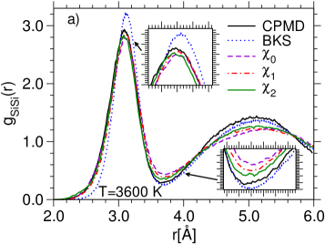
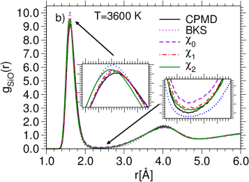
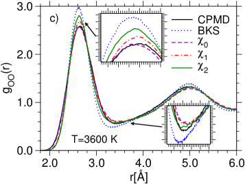
Figure 1: Partial pair distribution functions at $T=3600$ K computed using different sets of parameters (BKS, $\chi_{n},n\in\{0,1,2\}$) and compared to the CPMD results.

To calculate the cost function $\chi_{n}^{2}$ from Eq. (8), we need first to determine the functions $g_{\alpha\beta}(r;\bm{\xi})$. For this we have made an $NVT$ simulation at $T=3600$ K, using $N=1152$ atoms confined in a cubic box of $L=25.904$ Å, i.e. $\rho=2.2$ g/cm³. These simulations, with a time step of 1 fs, had a length of 10 ps. The first 20% of these runs were discarded since they might be affected by out-of-equilibrium effects (the starting configuration used for these MD runs corresponds to a SiO₂ melt equilibrated using another empirical potential, and hence the change in the effective potential will lead to an out-of-equilibrium situation.)

The search for the optimal set of parameters $\bm{\xi}$ has again been done by means of the Levenberg-Marquardt algorithm. Since this requires the derivative of $\chi_{n}^{2}$ with respect to the various $\xi_{i}$, and hence the variation of $g_{\alpha\beta}(r,\bm{\xi})$ with $\bm{\xi}$, we have determined the latter from a finite difference scheme:

$$\frac{\partial g_{\alpha\beta}(r;\bm{\xi)}}{\partial\xi_{i}}\approx\frac{g_{\alpha\beta}(r;\xi_{i}+\varepsilon_{i})-g_{\alpha\beta}(r;\xi_{i}-\varepsilon_{i})}{2\varepsilon_{i}}.$$ (10)

Here the variations $\varepsilon_{i}$ have to be chosen with care for two reasons: On the one hand, these variations must be sufficiently small so that the approximation of Eq. (10) remains accurate, i.e. that the finite difference is a good approximation of the derivative. On the other hand, a variation of the fitting parameters that is too small will make that the variation of $g_{\alpha\beta}(r,\bm{\xi})$ is very small and hence the right hand side of Eq. (10), which is subject to noise because of the finite length of the run, cannot be determined with sufficient precision. In practice, the choice of $\varepsilon_{i}$ will also depend on how the discretization of the distance $r$, needed to calculate the integral (9), are made. Indeed, a small spatial discretization grid will give rise to a larger statistical uncertainty per bin of the $g(r)$, whereas a bin size that is too large will give an inaccurate evaluation of the integral. To calculate the integral in Eq. (8), we have divided the distance $r$ in bins of width 0.02 Å. Given the length of the MD trajectory, it has been determined that a good choice for the $\varepsilon_{i}$’s is to take them on the order of a few percent of $\xi_{i}$. In Table 1 we have included in the last column also the parameters that have been used here. More details can be found in Ref. Carre_Phd .

At this point, the importance of the equilibration phase must be emphasized for the scanning the parameter space. Each change of $\bm{\xi}$ will make that the initial particle configuration will no longer be representative of an equilibrium situation, this means that the system first needs to be re-equilibrated. This re-equilibration has been achieved by replacing every 50 time steps the velocities of all the particles by ones that have been drawn from a Maxwell-Boltzmann distribution Andersen . This massive thermostatting is necessary since the change of the potential generates a quite strong out-of-equilibrium situation, and more gentle thermostats, like, e.g. Nosé-Hoover, are not very efficient in such situations. Only once the system is equilibrated, one can start measuring the structural quantities, such as the radial distribution functions, that are required to calculate the cost function.

Finally, we comment on the choice of the exponent $n$ in Eq. (8). Using the fitting procedure just described we have determined the optimal values for the parameters $\bm{\xi}$ by considering in the cost function of Eq. (8) three values of $n$: $n=0$, 1, and 2. With these three sets of optimized parameters we have carried out standard MD simulations and determined the partial pair distribution functions at $T=3600$ K. These functions are shown in Fig. 1. Also included in the figures are the $g_{\alpha\beta}(r)$ as predicted, for the same temperature, by the CPMD simulation and the BKS potential. A comparison of the different curves shows that the BKS potential gives a fair description of the CPMD data, but that it is definitively less accurate than the prediction of the three other potentials, notably in the vicinity of the main peaks. Furthermore, it can be observed that with increasing $n$, the differences of the corresponding $g_{\alpha\beta}(r)$ with the CPMD data increase at the main peak and decrease at the first minimum, a trend that is understandable since a larger $n$ implies that the cost function is more sensitive for larger $r$.

Figure 2: Angular distribution functions for the $\widehat{\mbox{OSiO}}$ and $\widehat{\mbox{SiOSi}}$ angles at $T=3600$ K as obtained from different potentials.

For probing the influence of $n$ on the structure it is also useful to study the average angle spanned by two particles that share a common neighbor. For the case of $\widehat{\mathrm{OSiO}}$ and $\widehat{\mathrm{SiOSi}}$, the corresponding distributions are shown in Fig. 2. (The meaning of the various peaks and shoulders will be discussed below but can also be found, e.g., in Ref. vollmayr96 .) From this figure we recognize that the distributions corresponding to the different values of $n$ agree all quite well with the data from the CPMD simulations. However, a closer inspection of the distributions, in particular the one for $\widehat{\mathrm{OSiO}}$ around the peak, shows that $n=1$ gives a slightly better description of the CPMD distribution than the other potentials. Since also the pair distribution function for $n=1$ is very similar to the one from the CPMD simulations, see Fig. 1, in the following part of the text the potential derived using the $\chi^{2}_{1}$ criterion will be referred as being the “CHIK potential” carre08 . We note that data labelled “$\chi_{1}$” in Figs. 1–2 correspond to preliminary tests, and, due to different run lengths, differences exist with respect to similar data labelled “CHIK potential” in the following sections (e.g. in Figs. 5–6).

II.4 New effective potentials

The values for the optimal parameters $\bm{\xi}$ that we have obtained from the force-matching approach derived following Eq. (1), and the CHIK potential are listed in Tab. 1. For the sake of comparison, we have also included the values of the BKS potential from Ref. bks . In order to understand better their similarities and differences, the three potentials and the corresponding forces are plotted in Fig. 3.

Parameter		BKS	FM	CHIK	$\epsilon_{i}$
qSi	[e]	2.4	1.3743	1.9104	0.075
AOO	[eV]	1388.7730	666.3	659.5	105
BOO	[Å-1]	2.76000	2.748	2.590	0.085
COO	[eV.Å6]	175.0000	41.6	26.8	13.125
ASiO	[eV]	18003.7572	26486.	27029.	540
BSiO	[Å-1]	4.87318	5.1842	5.1586	0.03
CSiO	[eV.Å6]	133.5381	145.4	148.0	4.1
ASiSi	[eV]	0.0	3976.7	3150.4	300
BSiSi	[Å-1]	0.0	2.794	2.851	0.03
CSiSi	[eV.Å6]	0.0	882.5	626.7	66

Table 1: Parameters of the various potentials having the functional form given by Eq. (3). The last column gives the values of $\epsilon_{i}$ used in Eq. (10) to calculate the partial derivatives.

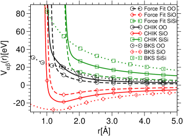
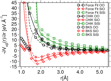
Figure 3: a) The $r-$dependence of the various effective potentials considered in this work. b) The corresponding forces.

Figure 3a gives the impression that the three potentials are qualitatively quite similar, and that only their absolute values are different. We point out, however, that it is not possible to make the different potentials coincide by a simple shift of the energy axis and we recall that 1 eV corresponds to 11600 K, thus the differences are in fact remarkably large. This can also recognized in Fig. 3b where we show the forces. In the range between 2-3 Å these forces differ by up to a factor of two, which shows that in fact the three force fields are very different. Furthermore, it can also be noted that the values of the various parameters for the three potentials are quite different: For example the charge of a silicon atom differs by 20%, and the prefactor $C_{\rm OO}$ of the van der Waals term varies by a factor of 6. In view of these large variations, we conclude that the problem of replacing the ab initio potential by an effective two-body potential is somewhat ill-posed and hence care has to be taken regarding the physical quantities (here forces or structure) used for determining the optimal parameters. Hence, it is important to check the quality of the obtained potentials by comparing its predictions for quantities that have not been used in the fitting procedure. This is done in the following section.

III Test of the potentials

In this section, we will first compare the predictions of the two effective potentials with the ab initio simulations results. As we will see, the potential obtained from the force matching gives structures that are rather different from the ones of the CPMD simulations and hence cannot be considered to be accurate. Hence, in the second part of this section the attention will be focused on the predictions of the CHIK potential, which seems to be quite reliable, the obtained structures will be compared with the ones predicted by the simulations of the CPMD and the BKS potentials.

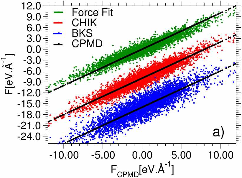
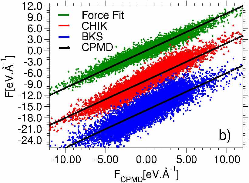
Figure 4: $x-$component of the force as obtained from the effective force fields as a function of the $x-$component of the CPMD force. The black straight lines are diagonals, i.e. correspond to a perfect correlation. Panels a) and b) show respectively the Si and O forces. For the sake of clarity the forces for the CHIK and BKS potentials have been shifted downwards by 8 eV/Å  and 16 eV/Å , respectively.

To start, we compare how, for a given configuration, the forces as predicted by the different potentials compare with the ones from the CPMD simulations. In Fig. 4, we show a scatter plot of the forces on a given particle as a function of the corresponding CPMD force. (Here we show the force in the $x$-direction, but the ones in $y$- and $z$-directions show of course qualitatively the same behavior). To calculate this scatter plot we have used all 100 configurations extracted from the CPMD run. If the effective potentials would indeed be able to reproduce reliably the CPMD forces, all the points should lie on the diagonal. We see that for the case of the FM potential the data points are indeed quite close to the diagonal, which shows that this approach is able to reproduce the CPMD forces with good accuracy. (Note that although the FM potential has been optimized such that the forces are well reproduced, it is a priori not evident that the functional form given by Eq. (3) is indeed able to give a good description of the forces).

Also included in Fig. 4 is the data obtained from the CHIK potential. We recognize that these forces deviate a bit more from the diagonal than the ones from the FM potential, which is no surprise since for the CHIK potential the information on the force was not taken into account for the optimization of the parameters. Despite this larger scattering, the correlation is still very satisfactory, giving thus evidence that this potential is indeed reliable.

In this figure we have included also the forces derived from the BKS potential and we see that these forces correlate significantly less with the CPMD forces that the ones from the two other potentials. This is somewhat surprising since in the past the BKS potential has been found to be quite reliable in predicting the properties of amorphous silica Horbach_thesis . Thus we can conclude that a good description of the forces on a given atom is not a necessary condition for a potential to give a good description of the material and later we will come back to this point. For the moment we thus just remark that it is satisfactory to see that the CHIK potential is able to give a better description of the forces than the BKS potential, even if this type of information has not been used at all for the optimization of its parameters. To quantify this trend we have calculated the $\chi^{2}_{F}$ as defined by Eq. (1) but now we have used on the right hand side the forces from the BKS and CHIK potentials. We have found that the corresponding values of $\chi_{F}^{2}$ are respectively 1.22 and 0.54, thus showing that quantitatively the forces have indeed improved significantly, even if they match the CMPD forces less good than the one from the FM potential (for which the $\chi_{F}^{2}$ was 0.17).

From Fig. 4, it can also be observed that in the oxygen scatter plot for the BKS as well as the CHIK potential the average slope is somewhat higher than unity. This indicates that for these potentials the large forces (in absolute value) are overestimated. This might be the reason why for these effective potentials the vibrational properties at intermediate and low frequencies are not very well reproduced Benoit02 .

In order to test the reliability of the FM and CHIK potential we have carried out a simulation of a $N=1152$ atoms system contained in a cubic box of size $L=24.904$ Å, which corresponds to a density of $2.2$ g/cm³. These simulations were done in the $NVT$ ensemble at a temperature of 3600 K using an Andersen thermostat Andersen . From the resulting configurations, we have then determined various structural quantities which allowed us to make a direct comparison of the structures obtained from the ab initio simulations with those obtained from the ones with the effective force fields.

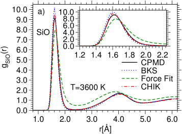
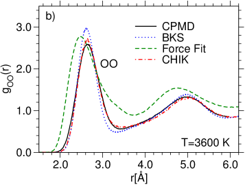
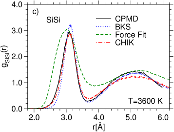
Figure 5: The different partial pair distribution functions at $T=3600$ K. The solid line corresponds to the ab initio simulations. The dotted and dashed-dotted lines show the results for the BKS and CHIK potential, respectively, and the dashed lines the one for the FM potential. The Inset in panel a) is a zoom onto the first peak.

.

In Fig. 5, we show the pair correlation functions from these simulations and compare them with the ones obtained from the CPMD simulations. The Si-O correlation function, Fig. 5a, shows that the BKS potential is able to give a good description of this correlation in that this function is very similar to the one from the CPMD. The main difference is seen in the first nearest neighbor peak in that the BKS potential overestimates its height by about 10%. For this peak, the CHIK potential gives a better description, in that the discrepancy is only about 5%. We also see that this potential is able to give an excellent description of the correlator in the vicinity of the first minimum, whereas in that region the BKS is slightly less accurate. For larger distances, the two effective potentials have a comparable accuracy. The perhaps most astonishing result of that figure is the curve for the FM potential in that we see that the correlator matches the CPMD curve extremely poorly. Thus, we can conclude already at this point that this potential is not able to reproduce the structure in a reliable manner, and in the final section this result will be commented further.

In Fig. 5b we show the O-O correlation function. Again we find that the curve from the BKS potential gives a good description of the CPMD data, but overestimates the height of the first peak and underestimates its width as well as the location of the first minimum. More accurate is the correlator of the CHIK potential in that the discrepancy regarding the height of the first peak is significantly reduced and also the first minimum as well as the second nearest neighbor peak are very similar to the one of the CPMD curve. The data from the FM deviates again very strongly from the CPMD curve.

The Si-Si pair correlation function, associated with the correlation that extends to the largest distance, is displayed in Fig. 5c. We see that the BKS potential gives a rather good description of the second nearest neighbor peak, but overestimates again the height of the first peak. The opposite trend is found for the CHIK potential in that the first peak matches very well the one from the CPMD simulations, but underestimates the height of the second peak. Also here the curve from the FM potential strongly deviates for all distances from the one of the CPMD simulation.

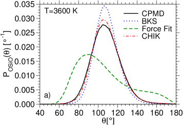
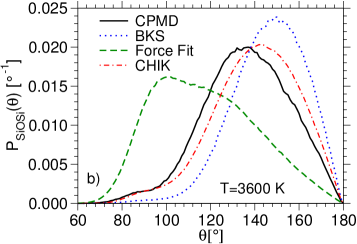
Figure 6: Comparison of the angular distribution functions derived from ab initio simulation, BKS and CHIK simulations and simulations using the FM potential at $T=3600$ K.

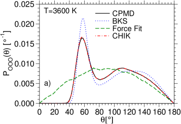
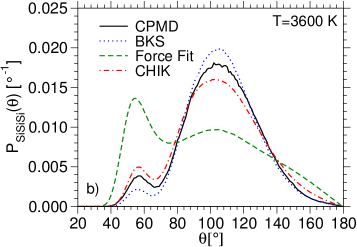
Figure 7: Angular distribution functions for the $\widehat{\mbox{OOO}}$ and $\widehat{\mbox{SiSiSi}}$ angles at $T=3600$ K computed using the CHIK and BKS potential and compared to the CPMD results..

After having discussed the two body correlation functions, we now present a comparison of the different potentials regarding a three point correlation function, i.e. an observable that characterizes the structure on a somewhat larger length scale. This is done by considering the distribution of the angles between three neighboring atoms, i.e. two atoms that are first nearest neighbor to the same central atom. In Fig. 6 and Fig. 7, we show the four most relevant combinations of such triplets. The most important one for the local structure is the angle $\widehat{\mathrm{OSiO}}$, see Fig. 6a, since it determines largely the shape of the tetrahedra. We note that the BKS potential as well as the CHIK potential reproduce well the peak around $106^{\circ}$, i.e. the typical angle in a tetrahedron, predicted by the CPMD simulations. The BKS potential overestimates the height of the peak by about 10% whereas for the CHIK potential this discrepancy is reduced to 6%. The distribution from the FM potential is very different from the one of the CPMD simulations and we conclude that this potential does not give rise to a realistic structure.

The angle $\widehat{\mathrm{SiOSi}}$ characterizes the relative arrangement of two neighboring tetrahedra. The corresponding distribution function is shown in Fig. 6b and we see that for this quantity the CHIK potential is significantly more reliable than the BKS potential in that the position and height of the main peak of the former are much closer to the one of the CPMD distribution than the ones of the latter. Also for this case the distribution for the FM potential is very different from the one of the CPMD.

The angle $\widehat{\mathrm{OOO}}$ gives information on the shape of a tetrahedron, as well as the relative orientation of two neighboring tetrahedra, and its distribution is shown in Fig. 7a. The first peak at $\theta=58^{\circ}$ corresponds to the angles made by three oxygen atoms belonging to the same tetrahedron. The height of this peak is significantly overestimated by the BKS potential indicating that this potential tends to generate structures that are too regular. As a consequence the second peak, located at $\theta\simeq 120-140^{\circ}$ and related to the oxygens on two neighboring tetrahedra, is lower and also flatter than the one predicted by the CPMD simulations. What is surprising in the figure is that the CHIK potential gives an almost perfect description of this distribution function. In contrast to this, the distribution from the FM potential is not good at all.

Finally, we show in Fig. 7b the distribution of the angle $\widehat{\mathrm{SiSiSi}}$, i.e. the angle between three neighboring tetrahedra. The graph shows that the BKS as well as the CHIK potential give a good although not perfect description of this distribution function. The position of the small peak at around $\theta\simeq 56^{\circ}$, which is due to three-membered rings see Ref. Rino , is reproduced well, but its height is over/underestimated by the CHIK and BKS potentials respectively. The main peak at around $\theta\simeq 104^{\circ}$ is due to larger rings and its height is again not reproduced very well, although its position is. Also in this case the prediction of the FM potential is not reliable.

So far we have checked to what extent the two effective potentials are able to reproduce the ab initio data at $T=3600$ K, i.e. at the temperature for which the various parameters characterizing these potentials have been optimized. However, it is of course also important to test whether these potentials are also capable to make reliable predictions at different temperatures, notably in the glass state. In the following we will thus present such tests. Since we have seen that the FM potential does a rather poor job in reproducing the CPMD data, for reasons that will be discussed in the final section, we will carry out these tests only for the CHIK potential and compare them with the results from the BKS potential.

Figure 8: Temperature dependence of the pressure as predicted by the BKS potential and for the CHIK potential with different cut-off radii for the short range part of the potential.

To this end, we start with the equation of state by monitoring how the pressure $P$ varies as a function of temperature if the density is kept fixed. We recall that silica has an anomaly in the density in that upon heating from low temperatures at constant pressure, its density first increases and only at intermediate and high temperatures it starts to decrease (or, if one considers heating of the system at constant volume, the pressure first decreases, before it starts to increase). In experiments, this anomaly, which is related to the open network structure of the system, is observed at around 1800 K bruckner . In Fig. 8 we show the temperature dependence of $P$ for the case of the BKS potential. In agreement with previous simulations at constant pressure vollmayr96 , one finds an anomaly at around 4800 K, i.e. the pressure dependence is qualitatively correct, but quantitatively the agreement is not that good. Also included in the figure is the result for the CHIK potential. We see that also this potential predicts an anomaly, although it is not very pronounced. On the other hand, the temperature at which this anomaly occurs is now shifted down to around 2200 K, i.e. relatively close to the temperature at which experiments show the maximum in the density.

Since Vollmayr et al. have found that the pressure depends quite strongly on the cut-off distance for the Buckingham terms of the interatomic potential vollmayr96 , it is of interest to check how this distance influences the equation of state for the CHIK potential. The result is included in Fig. 8 as well in that we show data for different values of this cut-off distance. We observe that changing this distance leads to a vertical shift of $P(T)$ that is basically independent of $T$. In particular we find that a decrease of $r_{\rm cut}$ by 1 Å leads to an increase of the pressure of about 1 GPa, whereas an increase of 2 Å makes that the pressure decreases by about 1 GPa. Thus in summary we can conclude that the choice of $r_{\rm cut}=6.5$ Å  is a very reasonable one.

Next, we study the structure of glasses produced with the various potentials. For this we have equilibrated a system of $1152$ atoms with the CHIK potential at $T=2440$ K and subsequently quenched it to $T=300$ K using a very high quench rate. To improve the statistics of the results we have repeated this procedure for 16 independent initial configurations.

We will compare the results with the data from three ab initio samples, discussed in Ref. Benoit02 , that have been obtained by quenching samples of the BKS potential to $300$ K and subsequently annealing them by means of a CPMD run of $0.7$ ps. Furthermore, we will also present data for the BKS potential. These glass structures have already been studied in Ref. vollmayr96 and have been obtained by cooling at constant pressure ($P=0$ GPa) ten systems of 1002 atoms with a quench rate of $4.44\times 10^{12}$ K/s to zero temperature.

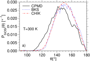
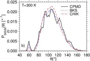
Figure 9: Angular distribution functions for the $\widehat{\mbox{SiOSi}}$, $\widehat{\mbox{SiSiSi}}$, and $\widehat{\mbox{OOO}}$ angles at $T=300$ K as obtained from the CHIK and BKS potentials and compared to the CPMD results.

Before we start with the comparison of the glass properties, we recall that these features do depend on the quench rate with which the glasses have been produced vollmayr96 . Therefore, one has to be careful if one compares the properties of glass samples that have been produced using very different cooling rates. However, these cooling rate effects are relatively small, depending on the observable considered on the order of 1-10% vollmayr96 , and hence are significantly smaller than the variation one gets by using different potentials (see below). Thus, in the following we will not discuss these cooling-rate effects.

In Fig. 9, we show the angular distribution functions as obtained from the three different potentials. The distribution of the $\widehat{\mbox{SiOSi}}$ angle is shown in panel (a) and we see that the one predicted by the BKS potential basically coincides with the one of the CHIK potential in that they both have a maximum at around 150^∘. A comparison with the corresponding distributions in Fig. 6 shows that the different maxima have shifted by $\Delta\theta^{\mathrm{CP}}\simeq 9^{\circ}$, $\Delta\theta^{\mathrm{BKS}}\simeq 4^{\circ}$, and $\Delta\theta^{\mathrm{CHIK}}\simeq 7^{\circ}$, indicating that the CHIK potential has a stronger $T-$dependence of the average angle than the BKS potential. Note that the experimental value for this angle, obtained from NMR data Mauri , is around 151^∘, thus it is in quite good agreement with the angle predicted by the CHIK and BKS potential. Surprisingly, this value is, however, larger than the one predicted by the CPMD data, $\theta^{\rm CP}_{\rm max}\simeq 145^{\circ}$. Thus, at this point one might start to wonder whether the CPMD simulation used to relax the glasses generated by the BKS potential Benoit02 ; Benoit_Ispas_1 are indeed able to anneal the structure in a significant manner. More studies on this point would certainly be very useful. Thus, if we assume that the distribution of this angle as predicted from the CPMD is not quite reliable and instead take the experimental value for the mean angle as a reference, we can conclude that the CHIK potential is indeed able to give a surprisingly good description of this angle for the glass at room temperature.

For the distribution of the angle $\widehat{\mbox{SiSiSi}}$, shown in Fig. 9b, we see that the BKS as well as the CHIK potential give results that are in good agreement with the CPMD data. However, due to the lack of statistics the latter is rather noisy and therefore it is at this point not possible to conclude much more from this agreement.

Regarding the $\widehat{\mbox{OOO}}$ distribution, shown in Fig. 9c, we can conclude that also here the agreement between the two effective potentials and the CPMD data is good, although both overestimate somewhat the height of the peak at around 60^∘. Since we have seen in Fig. 7b that at 3600 K the CHIK potential shows an excellent agreement with the CPMD data, we can thus conclude that this potential is able to give a good description of this angular distribution at several temperatures.

In experiments on atomic systems it is not possible to access in a direct way the partial pair distribution functions discussed above (Fig. 5). Instead one can sometimes measure their space-Fourier transforms, i.e. the partial structure factors $S_{\alpha\beta}({\bf q})$, where ${\bf q}$ is the wave-vector. However, in most cases these partial observables are also not accessible and only the neutron scattering function $S_{n}({\bf q})$, which is a weighted average over these partials, can be measured. This function is given by Lovesey

$$S_{n}({\bf q})=\frac{1}{N_{\rm{Si}}b_{\rm{Si}}^{2}+N_{\rm{O}}b_{\rm{O}}^{2}}\sum_{j=1}^{N}\sum_{k=1}^{N}b_{j}b_{k}\left\langle\exp\left[i{\bf q}\cdot({\bf r}_{j}-{\bf r}_{k})\right]\right\rangle.$$ (11)

Here the coefficients $b_{\alpha}$ with $\alpha\in\{\rm{Si,O}\}$ are the neutron scattering cross sections, $N_{\alpha}$ is the number of atoms of type $\alpha$ and $\langle\cdot\rangle$ is the thermal average. To calculate $S_{n}({\bf q})$ from the partial structure factors we have used the experimental values $0.4149\times 10^{-12}$ cm and $0.5803\times 10^{-12}$ cm for $b_{\rm{Si}}$ and $b_{\rm{O}}$, respectively nist .

The structure factor thus obtained from the different potentials is shown in Fig. 10. In this figure, the data from the BKS potential has been taken from Ref. horbach99 and the experimental data from Ref. Susman .

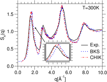
Figure 10: Comparison of the neutron scattering function from our simulation (red dashed line) with the experimental data of Susman et al. Susman (solid black line) and with simulation data with the BKS potential horbach99 (blue dotted line). The Inset shows a zoom on the first peak.

From this figure we see that the simulations with the effective potential are in quite good agreement with the experimental data. For the CHIK potential the position of the first peak, related to the nearest neighbor distance between two tetrahedra, reproduces the experimental value better than the BKS potential (see Inset), a trend that is very reasonable if one recalls the results on the radial distribution functions discussed above. Finally, we also note that the first peak, as well as the first minima are slightly over- and underestimated, respectively, indicating that the simulated structures are a bit too regular.

III.1 Vibrational density of states

So far we have mainly studied to what extent the effective potentials are able to reproduce the structural properties of the liquid and glass. However, many quantities that are relevant for practical applications do not depend on the geometry of the structure, but instead on the vibrational properties of the glass. Important examples for such quantities are the specific heat, the optical transmission coefficient, etc. It is therefore of interest to check whether the effective potentials are also able to reproduce the vibrational spectra, also called vibrational density of states (vDOS), of the system. We recall that this spectrum is given by the eigenvectors of the dynamical matrix, which is in turn directly related to the Hessian matrix, $\partial^{2}V/\partial{\bf r}_{i}\partial{\bf r}_{j}$. Thus, the vDOS can be considered as a measure on how accurate the potential is able to describe the local curvature of the potential in the vicinity of a local minimum, i.e. a glass state.

Previous studies on silica glasses have shown that ab initio simulations are able to reproduce quite reliably the vDOS as obtained from inelastic neutron scattering experiments Benoit02 ; Sarnthein ; giacomazzi ; haworth . This is also the case for the silica considered here and hence we can use the vDOS from the CPMD calculation as reference data.

In practice, we have determined the vDOS $g(\nu)$, where $\nu$ is the frequency, by using the glass configurations generated with the CHIK potential at 300 K (and from which we have obtained the structure of the glass discussed above) and started a standard $NVE$ simulation. By recording the velocity of all the particles, we calculated the Fourier transform of the mass-weighted velocity auto-correlation function. Within the harmonic approximation, which can be expected to hold at temperatures well below the glass transition temperature, this Fourier transform is then directly related to the vDOS via Dove

$$g(\nu)=\frac{1}{Nk_{B}T}\sum_{j}m_{j}\int_{-\infty}^{\infty}dt\langle{\bf v}_{j}(t)\cdot{\bf v}_{j}(0)\rangle\exp(i2\pi\nu t).$$ (12)

Note that by restricting in this relation the sum to only one species of particles, one can obtain the so-called partial vDOS which gives information on the vibrational behavior of a given species. The so obtained vDOS can be compared to the ab initio data published in Ref. Benoit02 and to the classical data obtained from the BKS potential vollmayr96 ; Horbach_thesis , see Fig. 11.

For the high frequency domain, $\nu>25$ THz, Sarnthein et al. have shown that the observed doublet is due to local vibrational modes of the SiO₄ tetrahedra, with the peak at $\nu=31.5$ THz being related to an out-of-phase motion of oxygen atoms in which two oxygen atoms move towards the central Si atom while the other two move away, and the peak at $\nu=35$ THz to an in-phase motion of all oxygen atoms toward the Si atom Sarnthein_Pasquarello . As can be seen in Fig. 11, the BKS predicts the location and intensity of these two peaks more accurately than the CHIK potential. This is not that surprising since in the parameterization of the BKS potential one has made use of the information of the vibrational modes located within one tetrahedron bks . In contrast to this, the CHIK potential does not have this kind of input and it is therefore a positive surprise that it is nevertheless able to reproduce these two peaks with a quite good quality.

The frequency range below $25$ THz shows a broad band that includes several peaks. We see that the CHIK potential gives a very good description of the high frequency edge of this band, and in particular it is in this $\nu-$range significantly more accurate than the BKS potential. The peak around $24$ THz, very pronounced in the CPMD data, is due to the bending of the Si-O-Si angle in the Si-O-Si plane Pasquarello98 . Although the CHIK potential underestimates somewhat the frequency of these excited states, it gets its intensity about right, and also in this case it fares better than the BKS potential.

For lower frequencies the vDOS of both classical potentials is relatively featureless and they are in fact very similar. This is in contrast to the CPMD data which show various peaks: The one at around 18 THz is related to modes associated with three-membered rings, and the one at around 12 THz to four-membered rings Pasquarello_Car . In agreement with previous studies, the classical potentials are not able to reproduce these spectral features and at present no obvious reason is known why this is so huang15 .

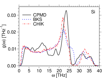
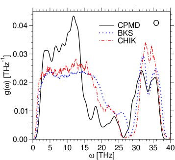
Figure 11: Partial vibrational density of states. The curves corresponding to the CHIK and BKS potentials have been determined using the velocity autocorrelation function at $T=300$ K on a sample with $N=1152$ and $N=8016$ atoms horbach99 , respectively. The ab initio data have been obtained at $0$ K by calculating the eigenvalues of the dynamical matrix on three $N=78$ atoms samples and by convoluting the resulting spectrum with a Gaussian broadening of width $2\sigma=1.05$ THz.

IV Summary and Conclusions

The goal of the presented work was to develop a method in which one uses the microscopic information provided by ab initio simulations to develop effective classical potentials. In addition, we wanted to compare our approach with the force matching method proposed by Ercolessi and Adams ercolessi94 since for certain systems this approach has given satisfactory results.

In the present approach, we started from the idea that if the effective potential is able to reproduce reliably the local arrangement of the atoms, it should give a good description of many other properties of the systems as well. Therefore, we have used the ab inito simulations at $T=3600$ K to calculate the partial radial distribution functions and then defined a cost function, Eq. (8), that characterizes how accurate an effective potential can reproduce these distribution functions. In a first step we have tested what choice should be done to define “local” by varying the exponent $n$ in Eq. (8) and found that $n=1$ is a good compromise since it gives a substantial weight to the structure at the first and second nearest neighbor distance.

Using this cost function we have optimized the parameters of the functional form given by Eq. (3) and obtained a new interaction potential (referred to as CHIK) for amorphous SiO₂. A comparison of the predictions of this new potential with the ones of the well studied BKS potential shows that for most structural properties the CHIK potential gives a better description of the CPMD data than the BKS potential, and that sometimes the improvement is quite significant. This superiority is found also in the equation of state in that the CHIK potential predicts a density anomaly at a temperature that is closer ($T=2300$ K) to the experimental value ($T=1823$ K) than the prediction of the BKS potential ($T=4800$ K). For the properties of the glass, we find that the CHIK potential predicts a structure that is in reasonably good agreement with the one from the ab initio simulations, and quite similar to the one of the BKS potential. In particular, it is remarkable that the vibrational vDOS of the CHIK potential shows the double peak feature at high frequencies, although this type of information has not been entered at all in the optimization of the parameters. We also mention that in Ref. carre08 we have discussed the temperature dependence of the diffusion constants and found that they are quite similar to the one of the BKS potential carre08 . In particular, they show at intermediate and low temperatures an Arrhenius dependence on temperature with an activation energy that is in good agreement with the experimental values for silica. Finally, we mention that we have also tested whether the CHIK potential is able to describe certain properties of crystalline data and found that, e.g., the elastic constants are reproduced quite well Carre_Phd . Further support that this potential is indeed quite reliable comes from other recent simulations in which one has studied amorphous silica at high pressures horbach08 ; zhang10 , its deformation at the nanoscale zheng10 , as well as the modeling of silica nanopores coasne11 ; cheng12 ; ori14 ; manga14 ; coasne14 and silica substrates ewers12 ; lepinay15 . Although a priori one cannot expect that the CHIK potential works well for these problems, since it has been derived with respect to the properties of bulk amorphous silica, in all these cases, the CHIK model has provided a reliable description. Thus we can conclude that the underlying idea of the presented fitting scheme works quite well in that the resulting potential is able to describe with good accuracy properties of the system that have not been used in the cost function.

Before we conclude we want to return to the surprisingly poor performance of the approach proposed by Ercolessi and Adams. In Fig. 4, we have seen that the effective potential obtained by the force matching method accurately reproduces the CPMD forces but that, Fig. 5, the resulting local structure is very different from the one predicted by the ab initio simulation. The reason for this apparent discrepancy lies, most probably, in the fact that the forces that act on the atoms of a local structure, say a tetrahedron, are highly correlated with each other and that there is in fact a large amount of compensations between these forces. The force matching method does not take into account this effect, making that the local residual forces are not necessarily small and thus in turn give rise to a local structure that can be very different from the one of the target (i.e. here the CPMD structure). For the case of a metal, where the forces are not covalent and much less directional, this effect can be expected to play a smaller role, thus rationalizing why for such systems the force matching method works significantly better than it is the case here ercolessi94 .

In summary, we can conclude from the present work that using the local structure as target for the optimization of the parameters of the potential is a very promising approach. As it is set up, the method gives a lot of freedom on the functional form that one wants to use, and thus one can of course also use, e.g., three body potentials. It is also possible to include in the cost function additional quantities, such as, e.g., elastic constants etc. The future will tell how useful the method will be for multi-component systems, but one can expect that as long as the number of parameters does not become too large, the approach will indeed allow to obtain reliable effective potentials.

- (1) K. Binder, J. Horbach, W. Kob, W. Paul, and F. Varnik, J. Phys.: Condens. Matter 16, S429 (2004).
- (2) D. Frenkel and B. Smit, Understanding Molecular Simulations: From Algorithms to Applications (Academic Press, San Diego, 2001).
- (3) W. Kob, Supercooled liquids, the glass transition, and computer simulations, in Lecture Notes for “Slow relaxations and nonequilibrium dynamics in condensed matter”, Les Houches July, 1-25, 2002; Les Houches Session LXXVII; Eds. J.-L. Barrat, M. Feigelman, J. Kurchan, and J. Dalibard (Springer, Berlin, 2003), p. 199-270.
- (4) P. J. Heaney, C. T. Prewitt, and G. V. Gibbs, Silica: physical behavior, geochemistry and materials applications, Rev. Mineral. 29 (Mineralogical Society of America, Washington, DC, 1994).
- (5) K. Binder and W. Kob, Glassy Materials and Disordered Solids: An Introduction to Their Statistical Mechanics (World Scientific, Singapore, 2011).
- (6) B. W. H. van Beest, G. J. Kramer, and R. A. van Santen, Phys. Rev. Lett. 64, 1955 (1990).
- (7) K. Vollmayr, W. Kob, and K. Binder, Phys. Rev. B 54, 15808 (1996).
- (8) M. Hemmati and C. A. Angell, J. Non-Cryst. Solids 217, 236 (1997).
- (9) J. Horbach and W. Kob, Phys. Rev. B 60, 3169 (1999).
- (10) J. Horbach, J. Phys.: Condens. Matter 20, 244118 (2008).
- (11) A. Carré, J. Horbach, S. Ispas, and W. Kob, Europhys. Lett. 82, 17001 (2008).
- (12) I. Saika-Voivod, H. M. King, P. Tartaglia, F. Sciortino, and E. Zaccarelli, J. Phys.: Condens. Matter 23, 285101 (2011).
- (13) B. Guillot and N. Sator, Geochim. Cosmochim. Acta 80, 51 (2012).
- (14) M. Tokuyama, J. Phys. Chem. B 115, 14030 (2011).
- (15) L. V. Woodcock, C. A. Angell, and P. Cheeseman, J. Chem. Phys. 65, 1565 (1976).
- (16) T. F. Soules, J. Chem. Phys. 71, 4570 (1979).
- (17) T. F. Soules, G. H. Gilmer, M. J. Matthews, J. S. Stolken, and M. D. Feit, J. Non-Cryst. Solids 357, 1564 (2011).
- (18) M. J. Sanders, M. Leslie, and C. R. A. Catlow, J. Chem. Soc., Chem. Commun. 1271 (1984).
- (19) M. Matsui and T. Matsumoto, Acta Cryst. B 41, 377 (1985).
- (20) M. Matsui, M. Akaogi, and T. Matsumoto, Phys. Chem. Minerals 14, 101 (1987).
- (21) A. C. Lasaga and G. V. Gibbs, Phys. Chem. Minerals 14, 107 (1987).
- (22) R. A. Jackson and C. R. A. Catlow, Mol. Simul. 1, 207 (1988).
- (23) B. P. Feuston and S. H. Garofalini, J. Chem. Phys. 89, 5818 (1988).
- (24) S. Tsuneyuki, M. Tsukada, H. Aoki, and Y. Matsui, Phys. Rev. Lett. 61, 869 (1988).
- (25) J. R. Chelikowsky, H. E. King, and J. Glinnemann, Phys. Rev. B 41, 10866 (1990).
- (26) P. Vashishta, R. K. Kalia, J. P. Rino, and I. Ebbsjö, Phys. Rev. B 41, 12197 (1990).
- (27) L. Sixtrude and M. S. T. Bukowinski, Phys. Rev. B 44, 2523 (1991).
- (28) G. J. Kramer, N. P. Farragher, B. W. H. van Beest, and R. A. van Santen, Phys. Rev. B 43, 5068 (1991).
- (29) K. P. Schröder, J. Sauer, M. Leslie, C. R. A. Catlow, and J. M. Thomas, Chem. Phys. Lett. 188, 320 (1992).
- (30) K. de Boer, A. P. J. Jansen, and R. A. van Santen, Chem. Phys. Lett. 223, 46 (1994).
- (31) K. de Boer, A. P. J. Jansen, and R. A. van Santen, Phys. Rev. B 52, 12579 (1995).
- (32) M. Wilson and P. A. Madden, J. Phys.: Condens. Matter 5, 2687 (1993).
- (33) M. Wilson, P. A. Madden, M. Hemmati, and C. A. Angell, Phys. Rev. Lett. 77, 4023 (1996).
- (34) S. Blonski and S. H. Garofalini, J. Am. Ceram. Soc. 80, 1997 (1997).
- (35) L. Duffrène and J. Kieffer, J. Phys. Chem. Solids 59, 1025 (1998).
- (36) E. Demiralp, T. Cagin, and W. A. Goddard III, Phys. Rev. Lett. 82, 1708 (1999).
- (37) P. Tangney and S. Scandolo, J. Chem. Phys. 117, 8898 (2002).
- (38) E. Flikkema and S. T. Bromley, Chem. Phys. Lett. 378, 622 (2003).
- (39) L. Huang and J. Kieffer, Phys. Rev. B 69, 224203 (2004).
- (40) V. V. Hoang, Eur. Phys. J. B 54, 291 (2006).
- (41) A. Pedone, G. Malavasi, M. C. Menziani, A. N. Cormack, and U. Segre, J. Phys. Chem. B 110, 11780 (2006).
- (42) S. Paramore, L. W. Cheng, and B. J. Berne, J. Chem. Theory Comput. 4, 1698 (2008).
- (43) D. Coslovich and G. Pastore, J. Phys.: Condens. Matter 21, 285107 (2009).
- (44) M. Benoit and W. Kob, Europhys. Lett. 60, 269 (2002).
- (45) R. D. Oeffner and S. R. Elliott, Phys. Rev. B 58, 14791 (1998).
- (46) M. Hawlitzky, J. Horbach, S. Ispas, M. Krack, and K. Binder, J. Phys.: Condens. Matter 20, 285106 (2008).
- (47) D. Marx and J. Hutter, Ab Initio Molecular Dynamics: Basic Theory and Advanced Methods (Cambridge University Press, Cambridge, 2009).
- (48) J. Kalikka, J. Akola, and R. O. Jones, Phys. Rev. B 90, 184109 (2014).
- (49) A. Bouzid, S. Gabardi, C. Massobrio, M. Boero, and M. Bernasconi, Phys. Rev. B 91, 184201 (2015).
- (50) L. Pedesseau, S. Ispas, and W. Kob, Phys. Rev. B, 91, 134201 (2015), Phys. Rev. B, 91, 134202 (2015).
- (51) R. A. Buckingham, Proc. R. Soc. A 168, 264 (1938).
- (52) R. Car and M. Parrinello, Phys. Rev. Lett. 55, 2471 (1985).
- (53) CPMD, Copyright IBM Corp 1990-2006, Copyright MPI für Festkörperforschung Stuttgart 1997-2001.
- (54) F. Ercolessi and J. B. Adams, Europhys. Lett. 26, 583 (1994).
- (55) D. R. Lide, Handbook of Chemistry and Physics, 82th edition (CRC Press, Boca Raton, 2002).
- (56) R. Martin, Electronic Stucture: Basic Theory and Practical Methods (Cambridge University Press, Cambridge, 2004)
- (57) G. B. Bachelet, D. R. Hamann, and M. Schlüter, Phys. Rev. B 26, 4199 (1982).
- (58) N. Troullier and J. L. Martins, Phys. Rev. B 43, 1993 (1991).
- (59) M. Benoit, S. Ispas, P. Jund, and R. Jullien, Eur. Phys. J. B 13, 631 (2000).
- (60) M. Benoit, S. Ispas, and M. E. Tuckerman, Phys. Rev. B 64, 224205 (2001).
- (61) S. Nosé, J. Chem. Phys. 81, 511 (1984).
- (62) W. G. Hoover, Phys. Rev. A 31, 1695 (1985).
- (63) G. J. Martyna, M. L. Klein, and M.E. Tuckerman, J. Chem. Phys. 97, 2635 (1992).
- (64) M. Pöhlmann, M. Benoit, and W. Kob, Phys. Rev. B 70, 184209 (2004).
- (65) J. Sarnthein, A. Pasquarello, and R. Car, Phys. Rev. Lett. 74, 4682 (1995).
- (66) M. Sprik, J. Phys. Chem. 95, 2283 (1991).
- (67) A. Carré, Development of Empirical Potentials for Amorphous Silica (VDM Verlag Dr. Müller, Saarbrücken, 2008).
- (68) W. H. Press, S. A. Teukolsky, W. T. Vetterling, and B. P. Flannery, Numerical Recipes in C The Art of Scientific Computing, 2nd Ed. (Cambridge University Press, Cambridge, 1992).
- (69) J.-P. Hansen and I. R. McDonald, Theory of Simple Liquids (Fourth Edition) (Academic Press, London, 2013).
- (70) H. C. Andersen, J. Chem. Phys. 72, 2384 (1980).
- (71) J. Horbach, Molekulardynamiksimulationen zum glasübergang von Silikatschmelzen (Ph. D. Thesis, Mainz, 1998).
- (72) J. P. Rino, I. Ebbsjö, R. K. Kalia, A. Nakano, and P. Vashishta, Phys. Rev. B 47, 3053 (1993).
- (73) R. Brückner, J. Non-Cryst. Solids, 5, 123 (1970).
- (74) F. Mauri, A. Pasquarello, B. G. Pfrommer, Y.-G Yoon, and S. G. Louie, Phys. Rev. B 62, R4786 (2000).
- (75) S. W. Lovesey, The Theory of Neutron Scattering from Condensed Matter, Vol. II (Oxford University Press, Oxford, 1986).
- (76) NIST: http://www.ncnr.nist.gov/resources/n-lengths/
- (77) S. Susman, K. J. Volin, D. G. Montague, and D. L. Price, Phys. Rev. B 43, 11076 (1991).
- (78) J. Sarnthein, A. Pasquarello, and R. Car, Science 275, 1925 (1997).
- (79) L. Giacomazzi, P. Umari, and A. Pasquarello, Phys. Rev. B 79, 064202 (2009).
- (80) R. Haworth, G. Mountjoy, M. Corno, P. Ugliengo, and R. J. Newport, Phys. Rev. B 81, 060301(R) (2010).
- (81) M. T. Dove, Introduction to Lattice Dynamics (Cambridge University Press, Cambridge, 1993).
- (82) A. Pasquarello, J. Sarnthein, and R. Car, Phys. Rev. B 57, 060301(R) 14133 (1998).
- (83) A. Pasquarello and R. Car, Phys. Rev. Lett. 80, 5145 (1998).
- (84) L. Huang and J. Kieffer, p. 87, in “Molecular Dynamics Simulations of Disordered Materials. From Network Glasses to Phase-Change Memory Alloys”, Editors: C. Massobrio, J. Du, M. Bernasconi, and P. Salmon, Springer Series in Materials Science 215 (Springer, Berlin, 2015).
- (85) C. Zhang, Z. H. Duan, and M. Y. Li, Geochim. Cosmochim. Acta 74, 4140 (2010).
- (86) K. Zheng, C. C. Wang, Y.-Q. Cheng, Y. H. Yue, X. D. Han, Z. Zhang, Z. W. Shan, S. X. Mao, M. M. Ye, Y. D. Yin, and E. Ma, Nature Comm. 1, 24 (2010).
- (87) B. Coasne, J. Haines, C. Levelut, O. Cambon, M. Santoro, F. Gorelli, and G. Garbarino, Phys. Chem. Chem. Phys. 13, 20096 (2011).
- (88) L. W. Cheng, J. A. Morrone, and B. J. Berne, J. Phys. Chem. C 116, 9582 (2012).
- (89) G. Ori, F. Villemot, L. Viau, A. Vioux, and B. Coasne, Mol. Phys. 112, 1350 (2014).
- (90) E. D. Manga, H. Blasco, P. Da-Costa, M. Drobek, A. Ayral, E. Le Clezio, G. Despaux, B. Coasne, and A. Julbe, Langmuir 30, 10336 (2014).
- (91) B. Coasne, C. Weigel, A. Polian, M. Kint, J. Rouquette, J. Haines, M. Foret, R. Vacher, and B. Rufflé, J. Phys. Chem. B 118, 14519 (2014).
- (92) B. W. Ewers and J. D. Batteas, J. Phys. Chem. C 116, 25165 (2012).
- (93) M. Lepinay, L. Broussous, C. Licitra, F. Bertin, V. Rouessac, A. Ayra, and B. Coasne, J. Phys. Chem. C 119, 6009 (2015).