Reconciling $(g-2)_{\mu}$ and charged lepton flavour violating processes through a doubly charged scalar

Abstract

The scalar particle discovered at the Large Hadron Collider (LHC) has properties very similar to that of a standard model (SM) Higgs boson. Limited experimental knowledge of its model origin, as of now, however, does not rule out the possibility of accommodating this new particle into a beyond the SM (BSM) framework. A few of these schemes suggest that the observed scalar is just the lightest candidate of an enriched sector with several other heavier states awaiting to be detected. Such models with nonminimal scalar sector also accommodate other neutral and electrically charged (singly, doubly, triply, etc.) component fields as prescribed by the specific model. Depending on the mass and electric charge, these new states can produce potential signatures at colliders as well as in low-energy experiments. The presence of a doubly charged scalar, when accompanied by other neutral or charged scalar(s), can also generate neutrino masses. Adopting the second scenario, e.g., Babu-Zee construction, constraints from neutrino physics have been effaced in this study. Here, we investigate a few phenomenological consequences of a uncoloured doubly charged scalar which couples to the charged leptons as well as gauge bosons. Restricting ourselves in the regime of conserved charged-parity (CP), we assume only a few nonzero Yukawa couplings ($y_{\mu\ell}$, where $\ell=e,\mu,\tau$) between the doubly charged scalar and the charged leptons. Our choices allow the doubly charged scalar to impinge low-energy processes like anomalous magnetic moment of muon and a few possible charged lepton flavour violating (CLFV) processes. These same Yukawa couplings are also instrumental in producing same-sign dilepton signatures at the LHC. In this article we examine the impact of individual contributions from the diagonal and off-diagonal Yukawa couplings in the light of muon $(g-2)$ excess. Subsequently, we use the derived information to inquire the possible CLFV processes and finally the collider signals from the decay of a doubly charged scalar. Our simplified analyses, depending on the mass of doubly charged scalar, provide a good estimate for the magnitude of the concerned Yukawa couplings. Our findings would appear resourceful to test the phenomenological significance of a doubly charged scalar by using complementary information from muon $(g-2)$, CLFV and the collider experiments.

I Introduction

Discovery of a new scalar Aad et al. (2012a); Chatrchyan et al. (2012a) has already proclaimed the success of LHC. This scalar has properties Aad et al. (2015a); atl (2015) quite identical to that of the SM Higgs boson, the only fundamental scalar within the SM framework. In the SM, the Higgs field emerges from an $SU(2)$ complex scalar doublet. A complete knowledge of the SM Higgs sector would require (i) measurements of the vacuum expectation value (VEV) acquired by the electrically neutral CP-even component of the aforementioned complex scalar doublet, (ii) the Higgs boson mass and (iii) the Higgs self coupling. At present, we have already probed the VEV of the SM through experimental measurements Olive et al. (2014) and, have estimated the mass of a Higgs-like scalar boson at the LHC Aad et al. (2015a). Thus, it remains to examine the only remaining parameter of the SM-Higgs sector, namely, the self-coupling. Unfortunately, the experimental sensitivity for the latter is very poor at the LHC and one perhaps needs to wait for the future colliders Baer et al. (2013). Hence, the possibility of having a Higgs-like scalar from BSM theories is certainly not redundant till date, especially when several other observations already ask for such an extension, e.g., nonzero neutrino masses and mixing Forero et al. (2012); Fogli et al. (2012); Gonzalez-Garcia et al. (2012). Furthermore, mass of the newly discovered scalar Aad et al. (2015a) and the top-quark mass Olive et al. (2014) strongly prefer the presence of one or more BSM scalars in the theory before $10^{9}-10^{11}$ GeV Sher (1989); Elias-Miro et al. (2012); Alekhin et al. (2012); Buttazzo et al. (2013) (see also Refs. Djouadi (2008a, b) for review). Introduction of these new scalars assures stability of the SM-Higgs potential up to the Planck scale. Combining these observations, an extension of the SM Higgs sector seems rather plausible. For example, one can add extra scalar states which are encapsulated in different multiplets guided by the gauge symmetry and/or pattern of the symmetry breaking. A plethora of analyses Pati and Salam (1974); Mohapatra and Pati (1975a, b); Senjanovic and Mohapatra (1975); Konetschny and Kummer (1977); Senjanovic (1979); Magg and Wetterich (1980); Schechter and Valle (1980); Cheng and Li (1980); Zee (1980); Lazarides et al. (1981); Mohapatra and Senjanovic (1981); Zee (1985); Georgi and Machacek (1985); Chanowitz and Golden (1985); Zee (1986); Babu (1988); McDonald (1994); Bento et al. (2000); Burgess et al. (2001); Babu and Macesanu (2003); Davoudiasl et al. (2005); Schabinger and Wells (2005); Cirelli et al. (2006); Kusenko (2006); Chen et al. (2007a); O’Connell et al. (2007); Bahat-Treidel et al. (2007); Chen et al. (2007b); Gogoladze et al. (2008); Barger et al. (2009); Hambye et al. (2009); Dawson and Yan (2009); Babu et al. (2009); Gonderinger et al. (2010); Aoki et al. (2011); del Aguila et al. (2012); Lebedev (2012); Elias-Miro et al. (2012); Chun et al. (2012); Chao et al. (2012); Bhupal Dev et al. (2013); Barry and Rodejohann (2013); Cline et al. (2013); Chakrabortty et al. (2014a, b); King et al. (2014); Okada et al. (2014); Costa et al. (2015); Martín Lozano et al. (2015); Falkowski et al. (2015); Bonilla et al. (2015a); Okada and Yagyu (2015); Das et al. (2015); Bambhaniya et al. (2015a) already exists in this connection where additional scalar mulitiplets are introduced to solve different shortcomings of the SM, like stability of the scalar potential up to the Planck scale, dark-matter, neutrino masses and mixing, etc.

These BSM scalar multiplets in general contain not only the electrically neutral fields but the charged (singly, doubly, triply, etc.) ones also. Phenomenology of these states may be constrained from the electroweak precision tests Olive et al. (2014), e.g., see Refs. Blank and Hollik (1998); Melfo et al. (2012); Chun et al. (2012); Bonilla et al. (2015b) for an extension with $SU(2)$ triplet Higgs. The presence of charged scalars, depending on the structure of the associated multiplet, at the same time can produce novel signals at the collider experiments, e.g., same-sign multileptons. Several analyses Gunion et al. (1996); Chakrabarti et al. (1998); Chun et al. (2003); Muhlleitner and Spira (2003); Akeroyd and Aoki (2005); Chen et al. (2007a); Han et al. (2007); Garayoa and Schwetz (2008); Kadastik et al. (2008); Akeroyd et al. (2008); Fileviez Perez et al. (2008); del Aguila and Aguilar-Saavedra (2009); Akeroyd and Chiang (2009); Maiezza et al. (2010); Akeroyd et al. (2010); Tello et al. (2011); Rentala et al. (2011); Aoki et al. (2011); Akeroyd and Sugiyama (2011); Melfo et al. (2012); Aoki et al. (2012); Akeroyd et al. (2012); Chakrabortty et al. (2012a); Das et al. (2012); Chun and Sharma (2012); Chen et al. (2013); Kanemura et al. (2013a); Bambhaniya et al. (2013); del Aguila et al. (2013); Chun and Sharma (2014); del Águila and Chala (2014); Bambhaniya et al. (2014a); Dutta et al. (2014); Kanemura et al. (2014a, b); Bambhaniya et al. (2014b); Deppisch et al. (2015); Han et al. (2015); Bambhaniya et al. (2015b) are already performed in this direction, including experimental ones Acton et al. (1992); Abbiendi et al. (2002); Abdallah et al. (2003); Abbiendi et al. (2003); Achard et al. (2003); Abazov et al. (2004); Acosta et al. (2004); Azuelos et al. (2006); Rommerskirchen and Hebbeker (2007); Hektor et al. (2007); Abazov et al. (2008); Aaltonen et al. (2008); Abazov et al. (2012); Aaltonen et al. (2011); Chatrchyan et al. (2012b); Aad et al. (2012b, 2015b). These charged scalars, apart from atypical LHC signatures, can also contribute to a class of low-energy phenomena that lead to lepton number as well as flavour violating processes. Such processes include CLFV (e.g. $\mu\to e\gamma,\,$ $\mu$ to $e$ conversion in atomic nuclei etc.) Petcov (1982); Leontaris et al. (1985); Bernabeu et al. (1986); Bilenky and Petcov (1987); Swartz (1989); Chun et al. (2003); Kakizaki et al. (2003); Cirigliano et al. (2004a, b); Abada et al. (2007); Fukuyama et al. (2010); Ren et al. (2011); Chakrabortty et al. (2012b); Dinh et al. (2012); Das et al. (2012); Barry and Rodejohann (2013); Nayak and Parida (2015); King et al. (2014); Borah et al. (2014); Deppisch et al. (2015), neutrinoless double beta decay ($0\nu\beta\beta$) Mohapatra and Vergados (1981); Haxton et al. (1982); Wolfenstein (1982); Hirsch et al. (1996); Cirigliano et al. (2004b); Chen et al. (2007a); Tello et al. (2011); del Aguila et al. (2012); Chakrabortty et al. (2012c); Barry and Rodejohann (2013); Bhupal Dev et al. (2015); King et al. (2014); Deppisch et al. (2015), rare meson decays (e.g., $M\to M^{\prime}\ell_{i}\ell_{j},\,M\to M^{\prime}\ell_{i}\ell_{j}\ell_{m}\ell_{n}$) Picciotto (1997); Ma (2009); Quintero (2013); Bambhaniya et al. (2015c), muon $(g-2)$ Fukuyama et al. (2010); Freitas et al. (2014) etc. Some of these processes, e.g., $0\nu\beta\beta$, rare-meson decays, etc. have one thing in common, i.e., they violate lepton number by $2$ units which is the characteristic of a doubly-charged scalar. The same doubly charged scalar can also participate in the CLFV processes and muon $(g-2)$. Several investigations, as aforesaid, do already exist concerning various phenomenological aspects of a doubly charged scalar. A dedicated entangled phenomenological inspection of the doubly-charged scalars, in the context of collider and low-energy experiments at the same time, however, still remains somewhat incomplete. This is exactly what we plan to do here and the current article is the first step toward a complete investigation. In passing we note that the other part of multiplets, i.e., the neutral scalar states can also show their own distinctive signals. For example, if these BSM neutral scalars are light, they can affect the SM-Higgs decay phenomenology through mixing. Phenomenological implications of additional neutral scalars are however, beyond the theme of this article and will not be addressed further.

We initiate our investigation with the discrepancy in anomalous magnetic moment of muon $\Delta a_{\mu}=a^{exp}_{\mu}-a^{th}_{\mu}$, which can be explained well in the presence of a doubly-charged scalar, $\Delta^{\pm\pm}$. Subsequently, we use this information to constrain only the most relevant associated Yukawa couplings that connect the doubly charged scalar with the charged leptons, i.e., $y_{\mu\ell}$ with $\ell=e,\,\mu,\,\tau$. In the next step, we investigate the allowed relevant CLFV processes in the presence of the same set of Yukawa couplings. At this level we scrutinize a new set of constraints on that same set of Yukawa couplings from the experimental limits on different CLFV processes. Finally, we explore the collider signals of a doubly charged scalar that appear feasible with the chosen set of Yukawa couplings and, are in agreement with the experimental constraints of $(g-2)_{\mu}$ and the relevant CLFV processes. However, like the existing literature we do not work in the context of any specific model. Rather, we parametrize the unknown model of doubly charged scalar in terms of a few relevant Yukawa couplings and the mass of the doubly charged scalar $(m_{\Delta^{\pm\pm}})$ that are resourceful to probe the existence of a doubly charged scalar experimentally. As a first attempt, we also stick to the regime of conserved CP. It is also important to emphasise that we focus on the range of $400~{}{\rm GeV}$ Aad et al. (2015b) $\raise 1.29167pt\hbox{$\;<$\kern-7.5pt\raise-4.73611pt\hbox{$\sim\;$}}m_{\Delta^{\pm\pm}}\raise 1.29167pt\hbox{$\;<$\kern-7.5pt\raise-4.73611pt\hbox{$\sim\;$}}1000~{}{\rm GeV}$ which is well accessible during run-II of the LHC. Thus, in a nutshell, in this work we explore the possible correlations among $m_{\Delta^{\pm\pm}}$ and $y_{\mu\ell}$ as well as between different $y_{\mu\ell}$ in the context of (i) $(g-2)_{\mu}$ and (ii) a few CLFV processes. Thereafter, we use these information to study the possible $\Delta^{\pm\pm}\to\ell^{\pm}_{\alpha}\ell^{\pm}_{\beta}$ processes (i.e., same-sign dileptons) at the LHC.

It remains to mention one more important aspect associated with a $\Delta^{\pm\pm}$, i.e., the generation of nonzero neutrino masses and mixing. Accommodating massive neutrinos in the presence of a $\Delta^{\pm\pm}$ depends on the chosen theory framework which we will discuss later in Sec. II. Models of these kinds typically contain additional scalars (neutral, charged or both, depending on the concerned model) and a larger set of Yukawa couplings. This nonminimal set of Yukawa couplings (compared to $y_{\mu\ell}$) is essential to accommodate massive neutrinos simultaneously with an explanation for the $(g-2)_{\mu}$ anomaly, in the presence of a few CLFV processes. In the context of a minimal model (described later), we observed that the set of constraints on the relevant Yukawa couplings coming from the anomalous $(g-2)_{\mu}$ and nonobservation of the CLFV processes is rather independent to the ones required to satisfy the observed three flavour global neutrino data Forero et al. (2012); Fogli et al. (2012); Gonzalez-Garcia et al. (2012).

The paper is organised as follows, after the introduction we present a concise description of the underlying theoretical framework in Sec. II. Analytical expressions for the muon $(g-2)$ and a few possible CLFV processes are given in Sec. III and Sec. IV, respectively. We present results of our numerical analyses on $\Delta a_{\mu}$ and the allowed CLFV processes in Sec. V. Collider phenomenology of the $\Delta^{\pm\pm}\to\ell^{\pm}_{\alpha}\ell_{\beta}^{\pm}$ processes, following findings of the previous section is addressed in Sec. VI. Our conclusions are given in Sec. VII. Finally, a detail computation of the anomalous magnetic moment of muon through a doubly charged scalar is relegated in the appendix.

II The theory framework

The presence of a doubly charged scalar is possible in various representations, for example (i) an $SU(2)$ triplet $\delta^{T}\equiv(\delta^{++},\,\delta^{+},\delta^{0})$ with hypercharge, $Y=1$ Konetschny and Kummer (1977); Senjanovic (1979); Magg and Wetterich (1980); Schechter and Valle (1980); Cheng and Li (1980), (ii) an $SU(2)$ singlet $\kappa^{++}$ with $Y=2$ Babu (1988); del Aguila et al. (2012); Gustafsson et al. (2013), (iii) left-right symmetric model Pati and Salam (1974); Mohapatra and Pati (1975a, b); Senjanovic and Mohapatra (1975), (iv) a quadruplet $\Sigma^{T}\equiv(\Sigma^{++},\,\Sigma^{+},\,\Sigma^{0},\,\Sigma^{-})$ with $Y=1/2$ Ren et al. (2011), (v) another doublet $\chi^{T}\equiv(\chi^{++},\,\chi^{+})$ with $Y=3/2$ Gunion et al. (1996); Rentala et al. (2011); Aoki et al. (2011); Yagyu (2013), (vi) a quintuplet $\Omega^{T}\equiv(\Omega^{++},\,\Omega^{+},\,\Omega^{0},\,\Omega^{-},\,\Omega^{--})$ with $Y=0$ etc. The mulitiplets $\Sigma$ and $\chi$ give rise to dimension-five while $\Omega$ produces dimension-six neutrino mass operators through their respective interactions with the SM fields. It is worth mentioning that a doubly charged scalar can also appear in a quintuplet with $Y>0$ or in multiplets with larger isospins Babu et al. (2009); Picek and Radovcic (2010); Kumericki et al. (2011); Ren et al. (2011); Bambhaniya et al. (2013); Earl et al. (2014).

Phenomenological aspects of these multiplets are constrained from the electroweak precision observables Georgi and Machacek (1985); Chanowitz and Golden (1985); Blank and Hollik (1998); Melfo et al. (2012); Hally et al. (2012); Chun et al. (2012); Hisano and Tsumura (2013); Kanemura et al. (2013b); Earl et al. (2013); Bonilla et al. (2015b), especially if the multiplet contains an electrically neutral component which develops a VEV. For the simplicity of analysis we however, focus solely on the doubly charged scalar without caring about the rest of multiplet members. This approach helps us to pin down the precise contributions from the doubly charged scalar. Furthermore, we assume negligible to vanishingly small VEV for the neutral scalar member of the associated multiplet, if any. The latter choice not only protects the $\rho$-parameter Olive et al. (2014), but also guarantees the absence and(or) severe suppression of some of the couplings, e.g., $\Delta^{\pm\pm}W^{\mp}W^{\mp}$.

We are now ready to write down the relevant terms for our analysis. For the purpose of $(g-2)_{\mu}$ one needs to consider only terms like $y_{\mu\ell}\Delta^{\pm\pm}\mu^{\mp}\ell^{\mp}$. All other Yukawa couplings are taken to be zero and further, we assume $y_{\mu\ell}=y_{\ell\mu}$ as well as $y_{\mu e}=y_{\mu\tau}$. One must remain careful while interpreting these $y_{\mu\ell}$ where information about the specific model (see Refs. del Aguila et al. (2013); del Águila and Chala (2014)) are also embedded. Our simplified choice of $y_{\mu\ell}$ leaves us with only three free parameters, namely $y_{\mu\mu},\,y_{\mu e}(=y_{\mu\tau})$ and $m_{\Delta^{\pm\pm}}$ relevant for our analysis. It is apparent from our choice of Yukawa couplings that, along with $(g-2)_{\mu}$, a few CLFV processes like $\mu\to e\gamma$, $\tau\to\mu\gamma$, $\mu N\to eN^{*}$ ($\mu$ to $e$ conversion in atomic nuclei) etc. are automatically switched on. We will elaborate this issue further in Sec. IV. Finally, we need to write down the relevant terms which lead to $pp\to\Delta^{\pm\pm}\Delta^{\mp\mp}$ process at the LHC. The necessary trilinear couplings between $\Delta^{\pm\pm}$ and the electroweak gauge-bosons, in the absence of VEV for the new multiplet, are given as del Águila and Chala (2014): $2ig_{2}\sin\theta_{W}\Delta^{\pm\pm}\Delta^{\mp\mp}A_{\sigma}p^{\sigma}$ and $i(g_{2}/\cos\theta_{W})(2-{Y}-2\sin^{2}\theta_{W})\Delta^{\pm\pm}\Delta^{\mp\mp}Z_{\sigma}p^{\sigma}$, where $p^{\sigma}$ is the momentum transfer at these vertices. Here, $Y$ is hypercharge of the scalar multiplet that contains $\Delta^{\pm\pm}$, $g_{2}$ is the $SU(2)$ gauge coupling and $\theta_{W}$ is Weinberg angle Olive et al. (2014). It is important to note the structure of $\Delta^{\pm\pm}\Delta^{\mp\mp}Z_{\mu}$ vertex, where some knowledge of the underlying multiplet appears necessary through the hypercharge quantum number.

Massive neutrinos with a $\Delta^{\pm\pm}$

In this subsection, as mentioned in the beginning, we aim to present a brief discussion about the neutrino mass generation in the presence of a $\Delta^{\pm\pm}$. Accommodating tiny neutrino masses in a model with $\Delta^{\pm\pm}$ can be achieved in different ways, e.g., in the tree-level from a Type-II seesaw mechanism using an $SU(2)$ triplet Konetschny and Kummer (1977); Senjanovic (1979); Magg and Wetterich (1980); Schechter and Valle (1980); Cheng and Li (1980) or in the loop-level with an $SU(2)$ singlet doubly and another $SU(2)$ singlet singly $(S^{+})$ charged scalar Babu (1988) etc. However, a $\Delta^{\pm\pm}$ gets directly involved in the mechanism of neutrino mass generation only for the latter model and thus, we restrict our discussion only for this framework.

It turns out for the aforesaid scenario, better known as the Babu-Zee model Zee (1980, 1985, 1986); Babu (1988), one needs a $S^{+}$ along with a $\Delta^{\pm\pm}$ to generate neutrino masses ($m_{\nu}$) in the two-loop level. Now, let us assume that $y^{s}_{\ell\ell^{\prime}},\,y^{d}_{\ell\ell^{\prime}}$ represent the generic real Yukawa couplings between the charged leptons and $S^{+},\,\Delta^{\pm\pm}$, respectively with the following property: $y^{s(d)}_{\ell\ell^{\prime}}=y^{s(d)}_{\ell^{\prime}\ell}$. At this point if we set the scale of new physics (i.e., masses of $S^{\pm},\,\Delta^{\pm\pm}$ ($m_{S^{\pm}},\,m_{\Delta^{\pm\pm}}$) and any other relevant parameter) $\sim\mathcal{O}(1$ TeV), just for an example, then following Ref. Babu (1988) one can extract the following conditions:

(i) $\sum y^{s}_{\mu\ell}y^{s}_{\ell\mu}+\sum y^{d}_{\mu\ell}y^{d}_{\ell\mu}\sim\mathcal{O}(10)$ (from $(g-2)_{\mu}$ Nyffeler (2014)),

(ii) $\sum y^{s}_{e\ell}y^{s}_{\ell\mu}+\sum y^{d}_{e\ell}y^{d}_{\ell\mu}\raise 1.29167pt\hbox{$\;<$\kern-7.5pt\raise-4.73611pt\hbox{$\sim\;$}}\mathcal{O}(0.001)$ (from $\mu\to e\gamma$ Adam et al. (2013)) and

(iii) $y^{d}_{\mu\mu}y^{s^{2}}_{\mu\tau}(y^{s^{2}}_{e\tau}+y^{s^{2}}_{\mu\tau}+y^{s^{2}}_{e\mu})/(y^{s^{2}}_{e\tau}+y^{s^{2}}_{\mu\tau})\sim 0.06$ and $(y^{s^{2}}_{e\tau}+y^{s^{2}}_{\mu\tau})y^{d}_{\tau\tau}\sim 2\times 10^{-4}$ (assuming $m_{\nu}\sim 0.1$ eV Ade et al. (2015)).

At this point, let us assume that only $y^{s}_{\mu\mu},\,y^{d}_{\mu\mu}$ are $\sim\mathcal{O}(1)$ while other associated $y^{s},\,y^{d}$ values remain at least $\raise 1.29167pt\hbox{$\;<$\kern-7.5pt\raise-4.73611pt\hbox{$\sim\;$}}0.1$. Now one can easily satisfy condition (i) with $y^{s}_{\mu\mu}\sim 3$ and $y^{d}_{\mu\mu}\sim 1$. These chosen values can safely coexist with condition (ii) as long as (at least) $y^{s}_{e\mu},\,y^{d}_{e\mu}$ $\raise 1.29167pt\hbox{$\;<$\kern-7.5pt\raise-4.73611pt\hbox{$\sim\;$}}0.001$ and $y^{s}_{e\tau},\,y^{d}_{e\tau}$ $\raise 1.29167pt\hbox{$\;<$\kern-7.5pt\raise-4.73611pt\hbox{$\sim\;$}}0.01$. With these estimations one can rewrite condition (iii), up to a good approximation, as: $y^{d}_{\mu\mu}y^{s^{2}}_{\mu\tau}\sim 0.06$ and $y^{s^{2}}_{\mu\tau}y^{d}_{\tau\tau}\sim 2\times 10^{-4}$. The former is trivially satisfied with $y^{d}_{\mu\mu}\sim 1$ and $y^{s}_{\mu\tau}\raise 1.29167pt\hbox{$\;<$\kern-7.5pt\raise-4.73611pt\hbox{$\sim\;$}}\mathcal{O}(0.1)$. The latter with $y^{s}_{\mu\tau}\raise 1.29167pt\hbox{$\;<$\kern-7.5pt\raise-4.73611pt\hbox{$\sim\;$}}\mathcal{O}(0.1)$ hints $y^{d}_{\tau\tau}\sim\mathcal{O}(0.01)$. Making the scale of new physics $\sim\mathcal{O}(500$ GeV) one can get similar results, however, with reduced upper bounds on the concerned Yukawa couplings.

Collectively, playing with a larger set of Yukawa couplings, e.g., imposing hierarchical structures between $y^{d}$ and $y^{s}$ as well as among different flavour indices, one can always satisfy all the three aforementioned criteria. It is evident from conditions (i) - (iii), that the constraints from neutrino mass simultaneously put bounds on the off-diagonal $y^{s}$ and diagonal $y^{d}$. On the contrary, limits from $(g-2)_{\mu}$ and CLFV processes constrain independently both the diagonal and off-diagonal $y^{s},\,y^{d}$ couplings. Thus, without emphasising the neutrino physics, one can safely work in a scenario when $y^{s}\to 0$. The remaining Yukawa couplings, namely $y^{d}$s, however, remain tightly constrained from the experimental limits on muon $(g-2)$ and CLFV processes. An analysis of the said kind, thus, provides maximum estimates for the associated $y^{d}$-type couplings. Any further attempt to add additional requirements for the same model, like neutrino mass generation, would only provide reduced upper bounds on the involved $y^{d}$s. Hence, for the rest of the work we keep on working with only $y_{d}$-type Yukawa couplings (henceforth read as $y_{\ell\ell^{\prime}}$), imposing a minimal structure essential to account for the muon $(g-2)$ anomaly. We note in passing that, unless compensated by the relative mass hierarchies, the contribution to muon $(g-2)$ from a $\Delta^{\pm\pm}$ normally exceeds the same from a $S^{\pm}$ since $\Delta^{\pm\pm}\Delta^{\mp\mp}\gamma$, $S^{\pm}S^{\mp}\gamma$ vertices are sensitive to the electric charges of the concerned fields.

III Muon $(g-2)$ with $\Delta^{\pm\pm}$

Precision measurements of the different low-energy processes always provide an acid test for the BSM theories. Observation of any possible disparity for these processes, compared to the corresponding SM predictions, provides a golden opportunity to explore as well as constrain various BSM models. The observed discrepancy in the anomalous magnetic moment of muon, $\Delta a_{\mu}$ is a very intriguing example of this kind.

In the SM, anomalous magnetic moment of muon is associated with the coupling $ig_{2}\sin\theta_{W}$ $\overline{\mu}\gamma^{\sigma}\mu A_{\sigma}$. However, even including the higher order contributions within the SM one can not explain the observed discrepancy $\Delta a_{\mu}=$ $a^{exp}_{\mu}$ Bennett et al. (2006); Roberts (2010) - $a^{th}_{\mu}$ Prades et al. (2009); Nyffeler (2010); Davier et al. (2011); Hagiwara et al. (2011). Here $a^{exp}_{\mu}$ is the experimentally measured value of $(g-2)_{\mu}$ and $a^{th}_{\mu}$ is the theoretical estimate of $(g-2)_{\mu}$ in the context of the SM. The latest numerical value following Ref. Nyffeler (2014) is given by

$$\Delta a_{\mu}=a^{exp}_{\mu}-a^{th}_{\mu}=(29.3\pm 9.0)\times 10^{-10}.$$ (1)

The presence of any possible BSM contribution will generally affect the $\mu\to\mu\gamma$ process at the loop level. In the presence of a $\Delta^{\pm\pm}$, the new BSM contributions to $(g-2)_{\mu}$ are shown in Fig. 1.

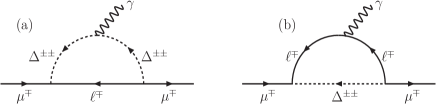
Figure 1: Possible Feynman diagrams showing contributions to the muon anomalous magnetic moment through the exchange of a doubly charged scalar and the selected $y_{\mu\ell}$. The arrows represent the direction of electric charge flow.

From this figure one can see that a $\Delta^{\pm\pm}$ can contribute to $(g-2)_{\mu}$ through two possible ways. Following Refs. Leveille (1978); Moore et al. (1985), new contribution to $(g-2)_{\mu}$, in the presence of $\Delta^{\pm\pm}$ and allowing all the charged leptons in the loop, is given by:

$$\Delta a_{\mu}=\frac{f_{m}m_{\mu}^{2}y_{\mu\ell}^{2}}{8\pi^{2}}$$

$$\times\Bigg{[}\int_{0}^{1}d\rho\,\,\frac{2(\rho+\frac{m_{\ell}}{m_{\mu}})(\rho^{2}-\rho)}{[m_{\mu}^{2}\rho^{2}+(m_{\Delta^{\pm\pm}}^{2}-m_{\mu}^{2})\rho+(1-\rho)m_{\ell}^{2}]}$$

$$-\int_{0}^{1}d\rho\,\,\frac{(\rho^{2}-\rho^{3}+\frac{m_{\ell}}{m_{\mu}}\rho^{2})}{[m_{\mu}^{2}\rho^{2}+(m_{\ell}^{2}-m_{\mu}^{2})\rho+(1-\rho)m_{\Delta^{\pm\pm}}^{2}]}\Bigg{]},$$ (2)

where $m_{\mu}$ is the mass of muon Olive et al. (2014) and $m_{\ell}$ is the mass of charged lepton $``\ell$”. We have also assumed real $y_{\mu\ell}$, so that $|y_{\mu\ell}|^{2}=y_{\mu\ell}^{2}$. Further details of the computation are relegated to the appendix. In Eq. (III), $f_{m}$ is equal to $1$ for $\ell=e,\,\tau$ while equals to $4$ for $\ell=\mu$. This multiplicative factor appears due to the presence of two identical fields in the interaction term.

IV CLFV and $\Delta^{\pm\pm}$

The most general Yukawa interactions between the charged leptons and a $\Delta^{\pm\pm}$ contains off-diagonal Yukawa couplings that are instrumental in producing CLFV processes like $\ell_{i}\to\ell_{j}\gamma$, $\ell_{a}\to\ell_{b}\ell_{c}\ell_{d}$ etc. In this article, however, we have assumed a minimal set of Yukawa couplings focusing on the muon anomalous magnetic moment. Thus, as already stated in Sec. II, our Yukawa sector contains only $y_{\mu\mu},\,y_{\mu e}$ and $y_{\mu\tau}$, with $y_{\mu e}=y_{\mu\tau}$. Such a parameter choice would allow only six CLFV processes, namely $\mu\to e\gamma,\,\tau\to e\gamma,\,\tau\to\mu\gamma,\,\tau\to 3\mu,\,\tau\to e\mu^{+}\mu^{-}$ and $\mu N\to eN^{*}$ at the respective leading orders, that too with only a few possible diagrams. For the clarity of reading, we describe all such diagrams in Fig. 2. At this stage, it appears crucial to explain the phrase “only six CLFV processes at the leading orders” in order to ameliorate any possible delusion. It is absolutely true that the chosen set of $y_{\mu\ell}$ forbids tree-level processes like $\mu\to 3e$, $\tau\to\mu e^{+}e^{-}$ through an off-shell $\Delta^{\pm\pm}$, as sketched for $\tau\to e\mu^{+}\mu^{-}$ process in diagram (e) of Fig. 2. All the relevant branching fractions $(Br)$ for the set of processes shown in Fig. 2 are given below Chun et al. (2003); Kakizaki et al. (2003); Akeroyd et al. (2009); Chakrabortty et al. (2012b):

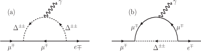
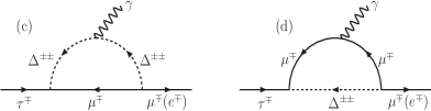
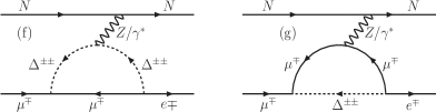
Figure 2: Possible Feynman diagrams showing contributions to $\mu\to e\gamma\,({\rm a,\,b}),\tau\to e\gamma,\tau\to\mu\gamma\,({\rm c,\,d}),\tau\to 3\mu,\tau\to e\mu^{+}\mu^{-}\,({\rm e})$ and $\mu N\to eN^{*}\,({\rm f,\,g})$ processes in the presence of a $\Delta^{\pm\pm}$ and the selected $y_{\mu\ell}$s. Here, $N$ represents the concerned atomic nucleus. The arrows represent the direction of electric charge flow.

$$Br(\mu\to e\gamma)=\frac{27\alpha_{em}|(yy^{\dagger})_{e\mu}|^{2}}{64\pi G_{F}^{2}m_{\Delta^{\pm\pm}}^{4}}~{}~{}Br(\mu\to e\bar{\nu}_{e}\nu_{\mu}),$$ (7)

$$Br(\tau\to e\gamma)=\frac{27\alpha_{em}|(yy^{\dagger})_{e\tau}|^{2}}{64\pi G_{F}^{2}m_{\Delta^{\pm\pm}}^{4}}~{}Br(\tau\to e\bar{\nu}_{e}\nu_{\tau}),$$

$$Br(\tau\to\mu\gamma)=\frac{27\alpha_{em}|(yy^{\dagger})_{\mu\tau}|^{2}}{64\pi G_{F}^{2}m_{\Delta^{\pm\pm}}^{4}}~{}Br(\tau\to\mu\bar{\nu}_{\mu}\nu_{\tau}),$$

$$Br(\tau\to 3\mu)=\frac{|y_{\tau\mu}|^{2}~{}|y_{\mu\mu}|^{2}}{4G_{F}^{2}m_{\Delta^{\pm\pm}}^{4}}~{}~{}Br(\tau\to\mu\bar{\nu}_{\mu}\nu_{\tau}),~{}{\rm and}$$

$$Br(\tau\to\mu\mu e)=\frac{|y_{\tau\mu}|^{2}~{}|y_{\mu e}|^{2}}{4G_{F}^{2}m_{\Delta^{\pm\pm}}^{4}}~{}~{}Br(\tau\to\mu\bar{\nu}_{\mu}\nu_{\tau}),$$

where $\alpha_{em}=g^{2}_{2}\sin^{2}\theta_{W}/4\pi$, $G_{F}$ is the Fermi constant Olive et al. (2014), $Br(\mu\to e\bar{\nu}_{e}\nu_{\mu})=100\%$, $Br(\tau\to e\bar{\nu}_{e}\nu_{\tau})=17.83\%$ and $Br(\tau\to\mu\bar{\nu}_{\mu}\nu_{\tau})=17.41\%$ Olive et al. (2014).

The rate of $\mu\to e$ conversion in atomic nuclei with the chosen set of $y_{\mu\ell}$ is written as

$$R(\mu N\to eN^{*})=\frac{(\alpha_{em}m_{\mu})^{5}Z_{\rm eff}^{4}Z|F(q)|^{2}}{4\pi^{4}m_{\Delta^{\pm\pm}}^{4}\Gamma_{\rm capt}}$$ (8)

$$\times\Big{|}\frac{y^{\dagger}_{e\mu}y_{\mu\mu}F(r,s_{\mu})}{3}-\frac{3(y^{\dagger}y)_{e\mu}}{8}\Big{|}^{2},{\rm where~{}}$$

$$F(r,s_{\mu}) ={\rm ln}~{}s_{\mu}+\frac{4s_{\mu}}{r}+(1-\frac{2s_{\mu}}{r})$$ (9)

$$\times\sqrt{(1+\frac{4s_{\mu}}{r})}~{}~{}{\rm ln}\frac{\sqrt{(1+\frac{4s_{\mu}}{r})}+1}{\sqrt{(1+\frac{4s_{\mu}}{r})}-1},$$

$$r=-\frac{q^{2}}{m_{\Delta^{\pm\pm}}^{2}},s_{\mu}=\frac{m_{\mu}^{2}}{m_{\Delta^{\pm\pm}}^{2}}.$$

Here, $Z$ is the atomic number of the concerned nucleus. Values of $Z_{\rm eff}$, $\Gamma_{\rm capt}$ and $F(q^{2}\backsimeq-m^{2}_{\mu})$ for the different atomic nuclei can be obtained from Ref. Kitano et al. (2002).

Finally, before we start discussing our results in the next section, we summarise the present and the expected future limits of the considered CLFV processes in Table 1.

CLFV processes	Present Limit	Future Limit
$\rm{BR}(\mu\rightarrow e\gamma)$	$5.7\times 10^{-13}$ Adam et al. (2013)	$6.0\times 10^{-14}$ Baldini et al. (2013)
$\rm{BR}(\tau\rightarrow e\gamma)$	$3.3\times 10^{-8}$ Aubert et al. (2010)	$3.0\times 10^{-9}$ Aushev et al. (2010)
$\rm{BR}(\tau\rightarrow\mu\gamma)$	$4.4\times 10^{-8}$ Aubert et al. (2010)	$3.0\times 10^{-9}$ Aushev et al. (2010)
$\rm{BR}(\tau\rightarrow 3\mu)$	$2.1\times 10^{-8}$ Hayasaka et al. (2010)	$1.0\times 10^{-9}$ Aushev et al. (2010)
$\rm{BR}(\tau\rightarrow e\mu^{+}\mu^{-})$	$2.7\times 10^{-8}$ Hayasaka et al. (2010)	$1.0\times 10^{-9}$ Aushev et al. (2010)
R($\mu N\rightarrow eN^{*}$)	$7.0\times 10^{-13}$ Bertl et al. (2006)	$2.87\times 10^{-17}$ Bartoszek et al. (2014)
(for ${\rm Au}$)

Table 1: The present and the expected future limits of the concerned CLFV processes.

V Results

We initiate exploring our findings with the muon anomalous magnetic moment in the context of BSM input parameters $m_{\Delta^{\pm\pm}}$ and $y_{\mu\ell}~{}(\equiv y_{\ell\mu})$. A self-developed FORTRAN code has been used for the purpose of numerical analyses. In our investigation we perform a scan over three free parameters $y_{\mu\mu}$, $y_{\mu e}(\equiv y_{\mu\tau})$ and $m_{\Delta^{\pm\pm}}$ in the following ranges: $10^{-4}\raise 1.29167pt\hbox{$\;<$\kern-7.5pt\raise-4.73611pt\hbox{$\sim\;$}}y_{\mu\mu},y_{\mu e}\raise 1.29167pt\hbox{$\;<$\kern-7.5pt\raise-4.73611pt\hbox{$\sim\;$}}1.2$ and $400~{}{\rm GeV}$ $\raise 1.29167pt\hbox{$\;<$\kern-7.5pt\raise-4.73611pt\hbox{$\sim\;$}}m_{\Delta^{\pm\pm}}\raise 1.29167pt\hbox{$\;<$\kern-7.5pt\raise-4.73611pt\hbox{$\sim\;$}}1000~{}{\rm GeV}$, respectively. For the analysis of $(g-2)_{\mu}$ we do not consider any constraints from the list of CLFV processes shown in Table 1. In Fig. 3, we plot the variation of $y_{\mu\mu}$ with $m_{\Delta^{\pm\pm}}$ when (i) only $y_{\mu\mu}$ is contributing to $\Delta a_{\mu}$ (left plot), that is $\ell$=$\mu$ in Fig. 1 and, (ii) all the chosen $y_{\mu\ell}$s are contributing to $\Delta a_{\mu}$ (right plot). The left plot of Fig. 3 shows a copacetic correlation between $m_{\Delta^{\pm\pm}}$ and $y_{\mu\mu}$, as expected for an analysis with only two free parameters [see Eq. (III) with $y_{\mu\ell}=0$ for $\ell\neq\mu$]. The smooth increase of $y_{\mu\mu}$ with larger $m_{\Delta^{\pm\pm}}$ values is also well understood from the same equation since $y_{\mu\mu}$ appears in the numerator while $m_{\Delta^{\pm\pm}}$ in the denominator. Hence, larger $y_{\mu\mu}$ values appear a must to satisfy the constraint on $\Delta a_{\mu}$ with increasing $m_{\Delta^{\pm\pm}}$. The blue and the green lines represent lower and upper bounds of the allowed one and two sigma (1$\sigma$-2$\sigma$) ranges for $\Delta a_{\mu}$ [see Eq. (1)], respectively. From the left plot one can also extract the possible range for $y_{\mu\mu}$, i.e., between $0.1-0.65$ when $m_{\Delta^{\pm\pm}}$ varies within $400~{}{\rm GeV}-1000$ GeV. The astonishing correlation between $y_{\mu\mu}$ and $m_{\Delta^{\pm\pm}}$ gets distorted when one switches on the other off-diagonal Yukawa couplings, namely $y_{\mu e}$ and $y_{\mu\tau}$, as shown in the right plot of Fig. 3. These distortions are apparent only for the upper bands of allowed one and two sigma $\Delta a_{\mu}$ values while the lower bands remain practically the same as the scenario with only $y_{\mu\mu}$. Two conclusions become apparent from the right plot of Fig. 3: (1) off-diagonal Yukawa couplings can produce significant contributions to $\Delta a_{\mu}$ and, (2) these new contributions are normally negative and thus, one needs larger $y_{\mu\mu}$ values to accommodate the $\Delta a_{\mu}$ data. At the same time, the similarity of the lower one and two sigma lines, in both of the plots, implies that contributions from the off-diagonal $y_{\mu\ell}$s are typically smaller compared to the same from $y_{\mu\mu}$. Unlike the left plot, here one does not get a smooth increase in $y_{\mu\mu}$ value with increasing $m_{\Delta^{\pm\pm}}$. One can however, still estimate a range for $y_{\mu\mu}$, i.e., $0.1-1.2$ for $400~{}{\rm GeV}\leq m_{\Delta^{\pm\pm}}\leq 1000~{}{\rm GeV}$.

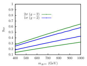
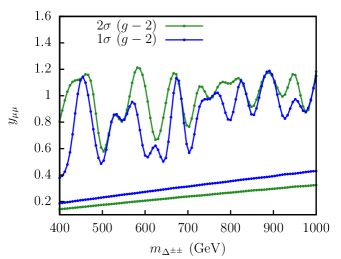
Figure 3: Correlations between $m_{\Delta^{\pm\pm}}$ and $y_{\mu\mu}$ for the allowed one and two sigma ranges of $\Delta a_{\mu}$. In the left plot $\Delta a_{\mu}$ is originating solely from $y_{\mu\mu}$ while in the right plot contributions from other off-diagonal $y_{\mu\ell}$s are also included. The blue and the green lines represent the one and two sigma bands of the allowed $\Delta a_{\mu}$ values, as given by Eq. (1).

In order to understand the relative contributions from $y_{\mu\mu}$ and $y_{\mu e},\,y_{\mu\tau}$ to the computation of $\Delta a_{\mu}$, we plot the four possible variations in Fig. 4. We consider the same range of $m_{\Delta^{\pm\pm}}$, i.e., $400~{}{\rm GeV}\raise 1.29167pt\hbox{$\;<$\kern-7.5pt\raise-4.73611pt\hbox{$\sim\;$}}m_{\Delta^{\pm\pm}}\raise 1.29167pt\hbox{$\;<$\kern-7.5pt\raise-4.73611pt\hbox{$\sim\;$}}1000~{}{\rm GeV}$ for these plots, similar to Fig. 3. All these data points (deep and light greens) satisfy the one and two sigma bounds on $\Delta a_{\mu}$ (represented by the light-brown and golden coloured bands, respectively), as given in Eq. (1). Two plots in the top row of Fig. 4 show the variations of $\Delta a^{y_{\mu\mu}}_{\mu}$ with respect to $y_{\mu\mu}$ and the off-diagonal Yukawa couplings. Two of the bottom row plots represent the same but for $|\Delta a^{y_{\mu e}+y_{\mu\tau}}_{\mu}|$. Here, $\Delta a^{y_{\mu\mu}}_{\mu}$ is that part of $\Delta a_{\mu}$ which arises solely from $y_{\mu\mu}$ while $|\Delta a^{y_{\mu e}+y_{\mu\tau}}_{\mu}|$ represents the same from $y_{\mu\ell}$ with $\ell\neq\mu$ [see Eq. (III)]. From the top-left plot of Fig. 4, it is evident that in the presence of off-diagonal Yukawas, $y_{\mu\mu}\raise 1.29167pt\hbox{$\;>$\kern-7.5pt\raise-4.73611pt\hbox{$\sim\;$}}0.3$ can yield a large contribution to muon $(g-2)$ beyond $2\sigma$. Thus, if we assume that contribution to $\Delta a_{\mu}$ arises solely from $y_{\mu\mu}$, i.e., $\Delta a_{\mu}\approx\Delta a^{y_{\mu\mu}}_{\mu}$, all points above the golden band remain experimentally excluded. The situation remains the same for $\Delta a^{y_{\mu\mu}}_{\mu}$ in the context of off-diagonal $y_{\mu\ell}$ when $y_{\mu e}$ or $y_{\mu\tau}\raise 1.29167pt\hbox{$\;>$\kern-7.5pt\raise-4.73611pt\hbox{$\sim\;$}}0.2$ (top-right plot for Fig. 4). Beyond $y_{\mu e}=0.2$, the sizeable but opposite $sign$ contributions (-$|\Delta a^{y_{\mu e}+y_{\mu\tau}}_{\mu}|$) from $y_{\mu\ell}$ adjust the positive over-growth of $\Delta a^{y_{\mu\mu}}_{\mu}$ beyond $2\sigma$ for $y_{\mu\mu}\raise 1.29167pt\hbox{$\;>$\kern-7.5pt\raise-4.73611pt\hbox{$\sim\;$}}0.3$, as shown in the bottom-right plot of Fig. 4. One more observation is apparent from the bottom-right plot of Fig. 4, that the contribution from $|\Delta a^{y_{\mu e}+y_{\mu\tau}}_{\mu}|$ in the determination of $\Delta a_{\mu}$ is practically negligible for $y_{\mu e}\raise 1.29167pt\hbox{$\;<$\kern-7.5pt\raise-4.73611pt\hbox{$\sim\;$}}0.01$. On the contrary, as can be seen from the bottom-left plot of Fig. 4, that $|\Delta a^{y_{\mu e}+y_{\mu\tau}}_{\mu}|$ shows hardly any sensitivity to $y_{\mu\mu}$ below $y_{\mu\mu}\raise 1.29167pt\hbox{$\;<$\kern-7.5pt\raise-4.73611pt\hbox{$\sim\;$}}0.3$. Only in the regime of $y_{\mu\mu}\raise 1.29167pt\hbox{$\;>$\kern-7.5pt\raise-4.73611pt\hbox{$\sim\;$}}0.3$, $|\Delta a^{y_{\mu e}+y_{\mu\tau}}_{\mu}|$ grows with $y_{\mu\mu}$. This growth becomes prominent for $y_{\mu\mu}\raise 1.29167pt\hbox{$\;>$\kern-7.5pt\raise-4.73611pt\hbox{$\sim\;$}}0.7$. So one can conclude that:

• (1) For the region $y_{\mu\mu}\raise 1.29167pt\hbox{$\;<$\kern-7.5pt\raise-4.73611pt\hbox{$\sim\;$}}0.3$, $y_{\mu e}(\equiv y_{\mu\tau})\raise 1.29167pt\hbox{$\;<$\kern-7.5pt\raise-4.73611pt\hbox{$\sim\;$}}0.01$, $\Delta a_{\mu}=\Delta a^{y_{\mu\mu}}_{\mu}+\Delta a^{y_{\mu e}+y_{\mu\tau}}_{\mu}\approx\Delta a^{y_{\mu\mu}}_{\mu}$. This is the reason why the lower one and two sigma lines for the two plots of Fig. 3 remain almost unaltered.

• (2) In a tiny region: $0.3\raise 1.29167pt\hbox{$\;<$\kern-7.5pt\raise-4.73611pt\hbox{$\sim\;$}}y_{\mu\mu}\raise 1.29167pt\hbox{$\;<$\kern-7.5pt\raise-4.73611pt\hbox{$\sim\;$}}0.7$, $0.01\raise 1.29167pt\hbox{$\;<$\kern-7.5pt\raise-4.73611pt\hbox{$\sim\;$}}y_{\mu e}(\equiv y_{\mu\tau})\raise 1.29167pt\hbox{$\;<$\kern-7.5pt\raise-4.73611pt\hbox{$\sim\;$}}0.2$, both of the contributions remain comparable to the measured $\Delta a_{\mu}$ [see Eq. (1)], i.e., $|\Delta a^{y_{\mu e}+y_{\mu\tau}}_{\mu}|\sim\Delta a^{y_{\mu\mu}}_{\mu}$ $\sim{\cal{O}}(\Delta a_{\mu})$. Hence, the measured constraint on $\Delta a_{\mu}$ appears feasible after a tuned cancellation between $\Delta a^{y_{\mu\mu}}_{\mu}$ and $\Delta a^{y_{\mu e}+y_{\mu\tau}}_{\mu}$.

• (3) Finally, in the region with $y_{\mu\mu}\raise 1.29167pt\hbox{$\;>$\kern-7.5pt\raise-4.73611pt\hbox{$\sim\;$}}0.7$, $y_{\mu e}(\equiv y_{\mu\tau})\raise 1.29167pt\hbox{$\;>$\kern-7.5pt\raise-4.73611pt\hbox{$\sim\;$}}0.2$, both of the contributions are larger than the measured $\Delta a_{\mu}$ (beyond the golden band at $2\sigma$ level). In other words, $|\Delta a^{y_{\mu e}+y_{\mu\tau}}_{\mu}|\sim\Delta a^{y_{\mu\mu}}_{\mu}$ $\gg{\cal{O}}(\Delta a_{\mu})$. Clearly, for this region, the parameter space that remains compatible with the measured constraint of $\Delta a_{\mu}$ appears through a much-tuned cancellation between $\Delta a^{y_{\mu\mu}}_{\mu}$ and $\Delta a^{y_{\mu e}+y_{\mu\tau}}_{\mu}$.

These last two features are also reflected in the erratic variation of $y_{\mu\mu}$, as shown in the right panel of Fig. 3.

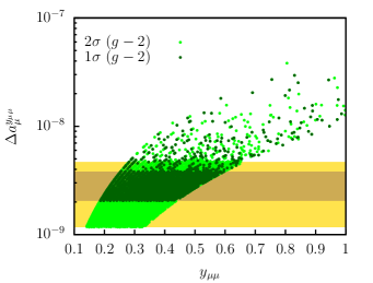
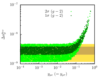
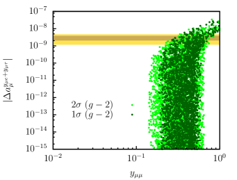
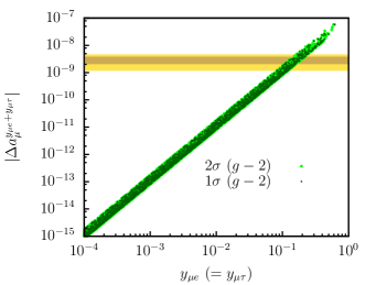
Figure 4: Plots showing variations of $\Delta a^{y_{\mu\mu}}_{\mu}$ with $y_{\mu\mu}$ (top-left), $y_{\mu e}(\equiv y_{\mu\tau})$ (top-right) and the changes of $|\Delta a^{y_{\mu e}+y_{\mu\tau}}_{\mu}|$ with $y_{\mu\mu}$ (bottom-left), $y_{\mu e}(\equiv y_{\mu\tau})$ (bottom-right). The quantities $\Delta a^{y_{\mu\mu}}_{\mu}$ and $|\Delta a^{y_{\mu e}+y_{\mu\tau}}_{\mu}|$ are explained in the text. The light-brown and golden coloured bands represent the measured $1\sigma$ and $2\sigma$ ranges of $\Delta a_{\mu}$ (see Eq. (1)). The deep-green (light-green) coloured point represents whether it satisfies the constraint on $\Delta a_{\mu}$ at the $1\sigma~{}(2\sigma)$ interval. We consider $400~{}{\rm GeV}\raise 1.29167pt\hbox{$\;<$\kern-7.5pt\raise-4.73611pt\hbox{$\sim\;$}}m_{\Delta^{\pm\pm}}\raise 1.29167pt\hbox{$\;<$\kern-7.5pt\raise-4.73611pt\hbox{$\sim\;$}}1000~{}{\rm GeV}$ for these plots.

A pictorial representation of these three aforesaid observations is shown in Fig. 5. Here, we plot the variations of individual components, i.e., $|\Delta a^{y_{\mu e}+y_{\mu\tau}}_{\mu}|$ and $\Delta a^{y_{\mu\mu}}_{\mu}$ with the total $\Delta a_{\mu}(\equiv\Delta a^{tot}_{\mu})$. It is apparent from this plot that the contribution of $\Delta a^{y_{\mu\mu}}_{\mu}$ in the evaluation of $\Delta a^{tot}_{\mu}$ is either the leading one (regime of overlap with the golden coloured band at the $2\sigma$ interval) or overshooting. On the other hand, for a novel region of the parameter space $|\Delta a^{y_{\mu e}+y_{\mu\tau}}_{\mu}|$ remains subleading (left-hand side of the golden coloured band) or comparable to $\Delta a^{y_{\mu\mu}}_{\mu}$ (regime of overlap with the golden band at the $2\sigma$ interval). Further, for $y_{\mu\ell}(\ell\neq\mu)\raise 1.29167pt\hbox{$\;>$\kern-7.5pt\raise-4.73611pt\hbox{$\sim\;$}}0.2$, $|\Delta a^{y_{\mu e}+y_{\mu\tau}}_{\mu}|$ can also overshoot $\Delta a^{tot}_{\mu}$ like $\Delta a^{y_{\mu\mu}}_{\mu}$ (right-hand side of the golden band). However, this excess is opposite in sign to that of the $\Delta a^{y_{\mu\mu}}_{\mu}$ and thus, together they respect the $2\sigma$ constraint on $(g-2)_{\mu}$.

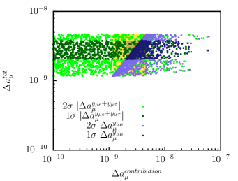
Figure 5: Plot showing variations of the individual components, i.e., $|\Delta a^{y_{\mu e}+y_{\mu\tau}}_{\mu}|$ and $\Delta a^{y_{\mu\mu}}_{\mu}$ with the total $\Delta a_{\mu}(\equiv\Delta a^{tot}_{\mu})$. The deep-green (light-green) coloured point represents whether it satisfies the constraint of $\Delta a_{\mu}$ at the $1\sigma~{}(2\sigma)$ interval for $|\Delta a^{y_{\mu e}+y_{\mu\tau}}_{\mu}|$. The deep-blue (light-blue) coloured points represent the same for $\Delta a^{y_{\mu\mu}}_{\mu}$. Remaining details are the same as Fig. 4.

The discussion presented so far in the context of $\Delta a_{\mu}$, using the information available from Fig. 3, Fig. 4 and Fig. 5, can be summarised as follows:

• (1) For most of the parameter space, the dominant contribution to $\Delta a_{\mu}$ is coming from $y_{\mu\mu}$, irrespective of $y_{\mu\ell}~{}(\ell\neq\mu)$ or $m_{\Delta^{\pm\pm}}$. This region is $y_{\mu e}(\equiv y_{\mu\tau})\raise 1.29167pt\hbox{$\;<$\kern-7.5pt\raise-4.73611pt\hbox{$\sim\;$}}0.01$, $0.1\raise 1.29167pt\hbox{$\;<$\kern-7.5pt\raise-4.73611pt\hbox{$\sim\;$}}y_{\mu\mu}\raise 1.29167pt\hbox{$\;<$\kern-7.5pt\raise-4.73611pt\hbox{$\sim\;$}}0.3$.

• (2) The contribution of $y_{\mu\ell}$ in $\Delta a_{\mu}$ is always negative and practically negligible till $y_{\mu\ell}\sim 0.01$. In the range of $0.01\raise 1.29167pt\hbox{$\;<$\kern-7.5pt\raise-4.73611pt\hbox{$\sim\;$}}y_{\mu\ell}\raise 1.29167pt\hbox{$\;<$\kern-7.5pt\raise-4.73611pt\hbox{$\sim\;$}}0.2$, $y_{\mu\ell}$ can yield a contribution to $(g-2)_{\mu}$ comparable to that from $y_{\mu\mu}$ (i.e., when $0.3\raise 1.29167pt\hbox{$\;<$\kern-7.5pt\raise-4.73611pt\hbox{$\sim\;$}}y_{\mu\mu}\raise 1.29167pt\hbox{$\;<$\kern-7.5pt\raise-4.73611pt\hbox{$\sim\;$}}0.7$) but with an opposite sign. Lastly, beyond $y_{\mu\ell}\sim 0.2$, a large negative contribution from this parameter helps to nullify the positive overshooting contribution to $\Delta a_{\mu}$ from $y_{\mu\mu}$ with $y_{\mu\mu}>0.7$.

• (3) Depending on the chosen range of $m_{\Delta^{\pm\pm}}$, i.e., $400~{}{\rm GeV}\raise 1.29167pt\hbox{$\;<$\kern-7.5pt\raise-4.73611pt\hbox{$\sim\;$}}m_{\Delta^{\pm\pm}}\raise 1.29167pt\hbox{$\;<$\kern-7.5pt\raise-4.73611pt\hbox{$\sim\;$}}1000~{}{\rm GeV}$, one can extract the upper bounds for the parameters $y_{\mu\mu}$ and $y_{\mu\ell}(\ell\neq\mu)$ from our analyses as $1.2$ [see right-panel plot of Fig. 3] and $0.6$ (see top-right plot of Fig. 4), respectively. These are the absolute possible upper limits of the respective parameters, as extracted through a simplified analysis. Adding other off-diagonal Yukawa couplings or introducing complex phases will in general result smaller upper bounds for the concerned parameters. The only trivial way to raise these bounds is to consider a higher $m_{\Delta^{\pm\pm}}$. This in turn would yield a smaller production cross-section for the process $pp\to\Delta^{\pm\pm}\Delta^{\mp\mp}$ at the LHC and thereby enhancing the possibility of escaping the detection.

The investigation of muon $(g-2)$ has given us some useful information about the parameters $y_{\mu\mu}$, $y_{\mu\ell}(\ell\neq\mu)$ and $m_{\Delta^{\pm\pm}}$. We are now in a perfect platform to analyse the importance of these parameters in the context of suitable and relevant CLFV processes, as given in Table 1. In order to perform this task, we do not consider the constraint from $(g-2)_{\mu}$. In this way, we can explore the other allowed corner of the parameter space for $y_{\mu\mu}$ and $y_{\mu\ell}$, focusing only on the CLFV processes. Subsequently, we will scrutinize mutual compatibility of the two allowed regions in $y_{\mu\mu}$ and $y_{\mu\ell}$ parameter space, as obtained from the $(g-2)_{\mu}$ and CLFV processes. However, to simplify our analysis we will use one key observation from our discussion of $\Delta a_{\mu}$, i.e., in general $y_{\mu\mu}>y_{\mu\ell}$.

The expressions for the branching fractions or the rate of different CLFV processes are given in Eqs. (7) – (8). From these formulas it is evident that the allowed region in $y_{\mu\mu}-y_{\mu\ell}$ parameter space, consistent with the bounds shown in Table 1, will expand with larger $m_{\Delta^{\pm\pm}}$ values. One can further extract another useful information from these expressions, i.e., $Br(\tau\to e\gamma)$ and $Br(\tau\to e\mu\mu)$ are the only two CLFV decays without any $y_{\mu\mu}$ contribution. Both of these processes are $\propto y^{2}_{\mu\ell}$ and thus, are in general suppressed compared to $Br(\tau\to\mu\gamma)$ and $Br(\tau\to 3\mu)$, respectively. At the same time, from the view point of present and the expected future limits (see Table 1), $Br(\tau\to e\gamma)$ $\sim{\cal{O}}$ $(Br(\tau\to\mu\gamma))$ and $Br(\tau\to e\mu\mu)$ $\sim{\cal{O}}$ $(Br(\tau\to 3\mu))$. Hence, one can safely neglect the constraints coming from those two processes on the $y_{\mu\mu}-y_{\mu\ell}$ parameter space without any loss of generality. The latter statement has also been verified numerically. Thus, we do not consider constraints from these two channels in our numerical analysis as they will not affect our conclusions anyway.

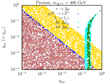
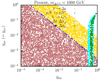
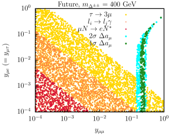
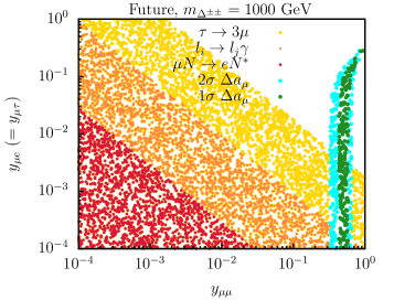
Figure 6: Plots showing variations of $y_{\mu\mu}$ with $y_{\mu e}~{}(\equiv y_{\mu\tau})$ in the context of CLFV processes: $\mu\to e\gamma$, $\tau\to\mu\gamma$ (collectively phrased as $\ell_{i}\to\ell_{j}\gamma$), $\tau\to 3\mu$, $\mu N\to eN^{*}$ and $\Delta a_{\mu}$. The plots of the top row are drawn for $m_{\Delta^{\pm\pm}}=400$ GeV (top-left) and $m_{\Delta^{\pm\pm}}=1000$ GeV (top-right) assuming the existing constraints on various CLFV processes (see Table 1). The sky-blue (deep-green) coloured point represents whether it satisfies the constraint of $\Delta a_{\mu}$ at the $2\sigma~{}(1\sigma)$ interval. The golden coloured points (for all the four plots) are those which satisfy the constraint of only $Br(\tau\to 3\mu)$. Deep-blue and dark-red colours (top-row) are used to represent those points which satisfy the constraint from only $\mu N\to eN^{*}$ process and only $\ell_{i}\to\ell_{j}\gamma$ process, respectively. The red and orange coloured points are used to represent the same two quantities in the bottom row plots. The plots of the bottom row are drawn using the expected future limits on different allowed CLFV processes.

We plot the allowed region of $y_{\mu\mu}-y_{\mu\ell}$ parameter space in Fig. 6 using the individual constraints on different CLFV processes as well as on $\Delta a_{\mu}$, adopting one at a time. Further, we consider two extreme values of $m_{\Delta^{\pm\pm}}$, i.e., $400$ GeV and $1000$ GeV which cover the entire span. This choice would help us to understand the relative modification of the surviving $y_{\mu\mu}-y_{\mu\ell}$ parameter space for a change in $m_{\Delta^{\pm\pm}}$ value. It is clear from all the plots of Fig. 6 that unlike $(g-2)_{\mu}$, the scales of $y_{\mu\mu}$ and $y_{\mu\ell}$ maintain some kind of reciprocal behaviour. This phenomenon is expected since all the formulas of Eqs. (7) – (8) contain the product of Yukawa couplings in the form of ($y_{\mu\mu}y_{\mu\ell}$). The relative arenas of the allowed $y_{\mu\mu}-y_{\mu\ell}$ regions for the different CLFV processes are also well understood. It is apparent from Table 1 that at present the most stringent limit is coming from $\mu\to e\gamma$, followed by $\mu N\to eN^{*}$. On the other hand, the CLFV tau decays have much larger lower bounds, ${\cal{O}}(10^{-8})$. Hence, as expected, the allowed $y_{\mu\mu}-y_{\mu\ell}$ parameter space for $\mu\to e\gamma$ (thus for $\ell_{i}\to\ell_{j}\gamma$) lies in the bottom (dark-red points in the top-row plots of Fig. 6). This region is followed by the survived $y_{\mu\mu}-y_{\mu\ell}$ parameter space from $\mu N\to eN^{*}$ process, since the present limit on $R(\mu N\to eN^{*})$ is marginally larger compared to the present bound on $Br(\mu\to e\gamma)$. This feature is evident from the narrow visible strip of blue coloured points as can be seen in both of the top-row plots of Fig. 6. Finally, rather high lower limit for $\tau\to 3\mu$ decay leaves a large allowed region in the $y_{\mu\mu}-y_{\mu\ell}$ space which is shown by the golden coloured points. The strip in the $y_{\mu\mu}-y_{\mu\ell}$ parameter space which respects the constraint of $\Delta a_{\mu}$ is very narrow and given by the sky-blue (dark-green) coloured points for the respective $2\sigma~{}(1\sigma)$ limit [see Eq. 1]. The presence of $m_{\Delta^{\pm\pm}}$ in the denominators [see Eqs. (7) – (8)] suggests an increase of the allowed $y_{\mu\mu}-y_{\mu\ell}$ parameter space with higher $m_{\Delta^{\pm\pm}}$ values. This behaviour is visible from the two top-row plots of Fig. 6 where the surviving $y_{\mu\mu}-y_{\mu\ell}$ region grows larger for $m_{\Delta^{\pm\pm}}=1000$ GeV (top-right plot) compared to $m_{\Delta^{\pm\pm}}=400$ GeV scenario (top-left plot). Independent study of the allowed CLFV processes and $(g-2)_{\mu}$ suggests that only a very narrow region of the $y_{\mu\mu}-y_{\mu\ell}$ parameter space can survive the combined constraints from both. This region is about $0.15-0.3$ for $y_{\mu\mu}$ while $0.0001-0.0004$ for $y_{\mu\ell}$ when $m_{\Delta^{\pm\pm}}=400$ GeV (top-left plot of Fig. 6). The span for $y_{\mu\ell}$ increases slightly, i.e., $0.0001-0.0008$ when one moves to $m_{\Delta^{\pm\pm}}=1000$ GeV (top-right plot of Fig. 6). The quantity $y_{\mu\mu}$, at the same time, just makes a small shift toward larger values, i.e., $0.3-0.6$ without expanding the allowed region.

The two plots in the bottom row of Fig. 6 trail more or less a similar discussion, especially in the context of $\Delta a_{\mu}$ for which the allowed $y_{\mu\mu}-y_{\mu\ell}$ parameter space remains the same. This is not true for other processes since these plots are made using the expected future sensitivities of the allowed CLFV processes (see Table 1). Now in the future, the quantity $R(\mu N\to eN^{*})$ is expected to achieve a lower limit which is about four orders of magnitude smaller than the current bound. On the contrary, future sensitivities for $\mu\to e\gamma$ process and CLFV tau decays are only one order of magnitude smaller than the existing ones. Thus, in the future the most stringent constraint on the $y_{\mu\mu}-y_{\mu\ell}$ parameter space would come from $R(\mu N\to eN^{*})$, as shown by the red coloured points in the two bottom-row plots. The next most severe constraint will appear from $\mu\to e\gamma$ (hence for $\ell_{i}\to\ell_{j}\gamma$) which is represented by orange coloured points. The golden coloured points represent the surviving $y_{\mu\mu}-y_{\mu\ell}$ region from the constraint of $\tau\to 3\mu$ process. Once again, for each of these concerned processes, a larger allowed region in the $y_{\mu\mu}-y_{\mu\ell}$ parameter space appears as we move from $m_{\Delta^{\pm\pm}}=400$ GeV (bottom-left plot) to $m_{\Delta^{\pm\pm}}=1000$ GeV (bottom-right plot). The relative shrink of the allowed parameter space while using improved future bounds, compared to that with the present constraints, is natural. However, the important observation from the bottom-row plots of Fig. 6 is the complete disappearance of the region of overlap between the surviving $y_{\mu\mu}-y_{\mu\ell}$ parameter spaces from $R(\mu N\to eN^{*})$ and $(g-2)_{\mu}$. The situation is practically the same for $Br(\mu\to e\gamma)$ and $(g-2)_{\mu}$, although a tiny region of overlap would remain for $m_{\Delta^{\pm\pm}}=1000$ GeV (bottom-right plot). A sizeable region of overlap will still exist between $Br(\tau\to 3\mu)$ and $(g-2)_{\mu}$ processes, however, smaller compared to the same with present constraints. So the region of $y_{\mu\mu}-y_{\mu\ell}$ parameter space that can survive the combined constraints from the possible CLFV processes and $(g-2)_{\mu}$ may disappear in the future. This missing area of overlap will certainly rule out the possibility of accommodating both the CLFV processes and $(g-2)_{\mu}$ in the context of a doubly charged scalar in the mass window of $400~{}{\rm GeV}\raise 1.29167pt\hbox{$\;<$\kern-7.5pt\raise-4.73611pt\hbox{$\sim\;$}}m_{\Delta^{\pm\pm}}\raise 1.29167pt\hbox{$\;<$\kern-7.5pt\raise-4.73611pt\hbox{$\sim\;$}}1000$ GeV. Nevertheless, one may observe a region of overlap like that of the top-row plots with larger values of $m_{\Delta^{\pm\pm}}$. The latter, as already stated, has rather less appealing collider phenomenology.

VI $\Delta^{\pm\pm}$ at the LHC

In this final section of our analysis we investigate the collider phenomenology of a $\Delta^{\pm\pm}$ in the light of LHC run-II. Our knowledge about the parameters $y_{\mu\mu},\,y_{\mu e}(\equiv y_{\mu\tau})$ and $m_{\Delta^{\pm\pm}}$, as we have acquainted in the last section thus, will appear resourceful. For the clarity of reading, it is important to reemphasise that so far we considered a few low-energy signatures solely from a $\Delta^{\pm\pm}$. Here, we study the pair-production of these $\Delta^{\pm\pm}$ having hypercharge $Y=1$ at the LHC and so, for our collider analysis. Thus, the coupling for $\Delta^{\pm\pm}\Delta^{\mp\mp}Z_{\sigma}$ vertex (see Sec. II) goes as $i(g_{2}\cos 2\theta_{W}/\cos\theta_{W})p^{\sigma}$. For other choices of the hypercharge one can simply scale this production cross-section, $\sigma(pp\xrightarrow{Z/\gamma}\Delta^{\pm\pm}\Delta^{\mp\mp})_{Y=1}$ as a function of $g_{2},\,Y$ and $\sin^{2}\theta_{W}$. Further, we also assume a negligible/vanishingly small VEV for the possible neutral scalar component of this $Y=1$ multiplet and hence, process like $\Delta^{\pm\pm}\to W^{\pm}W^{\pm}$ becomes irrelevant. In this scenario, the leading decay modes for a $\Delta^{\pm\pm}$ are $\ell^{\pm}_{\alpha}\ell^{\pm}_{\beta}$ which are controlled by $y_{\mu\mu}$ and $y_{\mu e}/y_{\mu\tau}$. It is thus apparent that a set of unconstrained $y_{\mu\ell}~{}(\ell=e,\,\mu,\,\tau)$ couplings will not only produce the same-sign same-flavour dileptons, e.g., $\Delta^{\pm\pm}\to\mu^{\pm}\mu^{\pm}$ but will also generate same-sign different-flavour dileptons, e.g., $\Delta^{\pm\pm}\to\mu^{\pm}e^{\pm},\,\mu^{\pm}\tau^{\pm}$ with equal branching fractions. The last two decays are example of lepton flavour violating scalar decays.

At this point, our knowledge of $y_{\mu\mu}$, $y_{\mu e}(\equiv y_{\mu\tau})$ and $m_{\Delta^{\pm\pm}}$ from Sec. V appears very meaningful to estimate the relative strengths of different possible $\Delta^{\pm\pm}\to\ell^{\pm}_{\alpha}\ell^{\pm}_{\beta}$ processes. For our collider analysis, just like our two previous investigations of a few CLFV processes and $(g-2)_{\mu}$, we consider $400~{}{\rm GeV}\raise 1.29167pt\hbox{$\;<$\kern-7.5pt\raise-4.73611pt\hbox{$\sim\;$}}m_{\Delta^{\pm\pm}}\raise 1.29167pt\hbox{$\;<$\kern-7.5pt\raise-4.73611pt\hbox{$\sim\;$}}1000$ GeV, following the exclusion limit set by the LHC run-I data-set Aad et al. (2015b). At the same time, from Sec. V, we can observe an allowed region in the $y_{\mu\mu}-y_{\mu\ell}(\ell\neq\mu)$ parameter space that survives the combined set of present constraints from muon $(g-2)$ and a few CLFV processes. In this region of survival, one gets $y_{\mu\ell}\sim{\mathcal{O}}(10^{-4})$ while $y_{\mu\mu}\sim{\mathcal{O}}(10^{-1})$ (see two top-row plots of Fig. 6). It is hence needless to mention that at the LHC processes like $\Delta^{\pm\pm}\to\mu^{\pm}e^{\pm}$ or $\Delta^{\pm\pm}\to\mu^{\pm}\tau^{\pm}$ will remain orders of magnitude suppressed compared to $\Delta^{\pm\pm}\to\mu^{\pm}\mu^{\pm}$ mode, provided one respects the combined constraints coming from $(g-2)_{\mu}$ and a few CLFV processes. Unfortunately, as discussed in Sec. V, such a conclusion would not hold true in the future when the $y_{\mu\mu}-y_{\mu\ell}(\ell\neq\mu)$ parameter space that can survive the combined constraints of $(g-2)_{\mu}$ and CLFV processes remains missing. One should note that such a region in the parameter space can reappear for large $m_{\Delta^{\pm\pm}}$ values, but at the cost of a diminished $\sigma(pp\xrightarrow{Z/\gamma}\Delta^{\pm\pm}\Delta^{\mp\mp})$. From the aforementioned discussion one can conclude that with our simplified parameter choice, the region of parameter space which respects the combined constraints of muon $(g-2)$ and some CLFV processes will predominantly yield four-muon ($pp\to\Delta^{\pm\pm}\Delta^{\mp\mp}\to 2\mu^{\pm}2\mu^{\mp}$) final state at the LHC.

For the sake of numerical analyses, the parton level signal events are generated using CalcHEP Belyaev et al. (2013). These events are then passed through PYTHIA v6.4.28 Sjostrand et al. (2006) for decay, showering, hadronization, and fragmentation. PYCELL has been used for the purpose of jet construction. We have used CTEQ6L parton distribution function Pumplin et al. (2002) while generating the events. Factorisation and renormalisation scales are set at $\sqrt{\hat{s}}$ (i.e, $\mu_{R}=\mu_{F}=\sqrt{\hat{s}}$), where $\sqrt{\hat{s}}$ is the parton level center-of-mass energy. We work in the context of LHC with 13 TeV center-of-mass energy and used the following set of basic selection cuts to identify isolated leptons ($l=e,~{}\mu$) and jets (hadronic) in the final states:

• (i) A final state lepton must have $p_{T}^{l}>10$ GeV and $|\eta^{l}|<2.5$.

• (ii) A final state jet is selected if $p_{T}^{j}>20$ GeV and $|\eta^{j}|<2.5$.

• (iii) Lepton-lepton separation, $\Delta R_{ll}>0.2$.

• (iv) Lepton-photon separation, $\Delta R_{l\gamma}>0.2$.

• (v) Lepton-jet separation, $\Delta R_{lj}>0.4$.

• (vi) Hadronic energy deposition, $\sum p^{had}_{T}$ around an isolated lepton must be $<0.2\times p_{T}^{l}$.

• (vii) Final states with four-leptons are selected if the leading and subleading leptons have $p_{T}^{l}>30$ GeV while for the remaining two, $p_{T}^{l}>20$ GeV.

Leading SM background contribution will arise from $t\bar{t}Z/\gamma^{*}$ or $ZZ/\gamma^{*}$ events. However, one can use the two following characteristics to suppress these backgrounds: (1) Four-lepton final states from $t\bar{t}Z/\gamma^{*}$ channels always appear with certain amount of missing transverse energy (${E\!\!\!\!/_{T}}$). (2) The set of four-leptons coming from $ZZ$ process contains pairwise same flavour opposite-sign leptons from a $Z$-decay, and can easily be eliminated using appropriate invariant mass ($m^{inv}$) cuts which is isomorphic to $Z-veto$. Background events are generated using MadGraph5@aMCNLO v$2.2.3$ Alwall et al. (2011, 2014) and subsequently showered with PYTHIA. In our background simulations, we switched on all the possible processes that lead to $pp\to 2\mu^{\mp}2\mu^{\pm}$ final state with at most two jets (light or $b$-tagged). At this stage, after a careful scrutiny of the different kinematic distributions for both the signal $(S)$ and background $(B)$ events, we have introduced the following set of advanced cuts to guarantee an optimized signal to background event ratio:
$C1$: Within the chosen framework a $\Delta^{\pm\pm}$ decays only into $\mu^{\pm}\ell^{\pm}~{}(\ell=e,\,\mu,\,\tau)$ and hence, one would expect no hadronic jets for the final states. However, hadronic jets may appear while showering and we therefore, limit the final state hadronic jet multiplicity up to one.
$C2$: We further impose another criterion on the possible final state hadronic-jet, i.e., it must not be a $b$-tagged jet. This choice helps to reduce the $t\bar{t}Z/\gamma^{*}$ background.
$C3$: Theoretically, no source of ${E\!\!\!\!/_{T}}$ exists for the predominant decay mode $\Delta^{\pm\pm}\to\mu^{\pm}\mu^{\pm}$ although nonzero ${E\!\!\!\!/_{T}}$ can appear from subleading $\Delta^{\pm\pm}\to\mu^{\pm}\tau^{\pm}$ mode. The latter, as discussed in the Sec. V, remains highly suppressed. Hence, we consider an upper limit of 30 GeV on the ${E\!\!\!\!/_{T}}$.
$C4$: In our analysis, a pair of same-sign leptons emerges from a $\Delta^{\pm\pm}$ whereas for the backgrounds, a pair of opposite-sign leptons shares the same source. We therefore, construct $m^{inv}$ for all the possible final state opposite-sign lepton pairs and discard all those events with $|m^{inv}_{l^{+}l^{-}}-m_{Z}|\leq 15$ GeV. Here, $m_{Z}$ is the mass of $Z$-boson. This cut appears useful to suppress backgrounds from $Z$-boson decay.

Benchmark	Parameters		Production	Cross-section
Points	$m_{\Delta^{\pm\pm}}$ (GeV)	$y_{\mu\mu}$	cross-section	after cuts
			(fb)	(fb)
BP1	600	0.29	1.52	0.286
BP2	800	0.46	0.33	0.061
BP3	1000	0.47	0.08	0.014
SM backgrounds	All inclusive		11.56	0.01

Table 2: Signal cross-sections for the three chosen benchmark points before and after applying the selection-cuts as described in the text. The final row represents the total cross-section from all the possible SM backgrounds which contain four-muon final states with a maximum hadronic-jet multiplicity of two.

In Table 2, we show the signal cross-sections prior and after implementing all the basic and advanced cuts. In this context, following the discussion of last section, we consider a set of three representative benchmark points which simultaneously satisfies the present set of bounds on CLFV processes and $(g-2)$ of muon. The same discussion also predicts $y_{\mu\mu}\gg y_{\mu\ell}(\ell\neq\mu)$ with $y_{\mu\mu}\sim{\cal{O}}(0.1)$ and $y_{\mu\ell}\sim{\cal{O}}(10^{-4})$. Thus, we do not explicitly mention the corresponding values of $y_{\mu e}(\equiv y_{\mu\tau})$ in Table 2. In the context of numbers presented in Table 2, it is interesting to explore the effectiveness of the advanced cuts, e.g., C3, C4. We have observed that the advanced selection cut C3 reduces 22% of the background events while diminishes 18% of the signal events (BP1 for example). Subsequent application of cut C4 kills 4% of the surviving events for the signal (BP1) whereas removes 99% of the surviving background events.

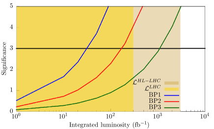
Figure 7: Variation of the statistical significance as a function of the integrated luminosity $(\mathcal{L})$ for the three different benchmark points (see Table 2). The black coloured horizontal line represents a $3\sigma$ statistical significance. The golden (dark-golden) coloured band represents the luminosity range (with a chosen lower limit of 1 fb^-1) for the LHC (proposed high luminosity LHC, HL-LHC).

Finally, in Fig. 7 we show the variation of statistical significance as a function of the integrated luminosity $(\mathcal{L})$, for a set of three possible benchmark points (see Table 2). The integrated luminosity range (starting from 1 fb^-1 up to the proposed maximum) for the LHC and the high-luminosity LHC (HL-LHC) hig ) are represented with golden and dark-golden colour, respectively. The horizontal black coloured line represents a $3\sigma$ statistical significance. The diminishing nature of statistical significance with increasing $m_{\Delta^{\pm\pm}}$ (see benchmark points in Table 2) is a natural consequence of reducing $\sigma(pp\to\Delta^{\pm\pm}\Delta^{\mp\mp})$. One can compensate this reduction with a higher center-of-mass energy or larger $\mathcal{L}$, as can be seen from Fig. 7. It is evident from this figure that one would expect strong experimental evidence (statistical significance $\geq 4\sigma$) of a $\Delta^{\pm\pm}$ (as sketched within our construction) up to $m_{\Delta^{\pm\pm}}\approx 800$ GeV during the ongoing LHC run-II. The exact time line is however, $m_{\Delta^{\pm\pm}}$ dependent. For example, a discovery (statistical significance $\geq 5\sigma$) of the studied $\Delta^{\pm\pm}$ up to $m_{\Delta^{\pm\pm}}\approx 600$ GeV appears possible with $\mathcal{L}=100$ fb^-1, which is well envisaged by 2017 – 2018. A similar conclusion for $m_{\Delta^{\pm\pm}}=800$ GeV at the $4\sigma$ level however, needs $\mathcal{L}=300$ fb^-1 and hence, could appear feasible around 2020. For a more massive $\Delta^{\pm\pm}$ discovery, e.g., $m_{\Delta^{\pm\pm}}=1000$ GeV, one would undoubtedly require a larger $\mathcal{L}$ like $3000$ fb^-1. Necessity of such a high $\mathcal{L}$ would leave a massive $\Delta^{\pm\pm}$ undetected at the LHC. The proposed high-luminosity extension of the LHC, HL-LHC hig , however, will certainly explore this scenario. We note in passing that a $\Delta^{\pm\pm}$ much heavier than $1000$ GeV would remain hidden even in such a powerfull machine. The latter, however, will leave its imprints through a region in the $y_{\mu\mu}-y_{\mu\ell}(\ell\neq\mu)$ parameter space (see Fig. 6) that would simultaneously respect the improved future bounds on a few CLFV processes and muon $(g-2)$.

VII Summary and Conclusions

Discovery of a “Higgs-like” scalar at the LHC and hitherto incomplete knowledge about its origin have revived the quest for an extended scalar sector beyond the SM. An interesting possibility is to consider these extensions through different spin-zero multiplets that contain various electrically charged (singly, doubly, triply etc.) and often also neutral fields. In this paper we have entangled the CLFV and muon (g-2) data to constrain the relevant parameters associated with a doubly charged scalar through a simplified structure and also discuss the possible collider signatures. Further, focusing on the muon anomalous magnetic moment, we have assumed only a few nonzero Yukawa couplings, namely $y_{\mu\ell}$ with $\ell=e,\,\mu,\,\tau$, between the doubly charged scalar and the charged leptons. Furthermore, for simplicity we have chosen them real as well as $y_{\mu e}=y_{\mu\tau}$ and thus, left with only three relevant free parameters, namely $y_{\mu\mu},\,y_{\mu e}(\equiv y_{\mu\tau})$ and $m_{\Delta^{\pm\pm}}$.

This simplified framework gives two additional contributions to the muon anomalous magnetic moment, as shown in Fig. 1. To start with we have computed contributions of these two new diagrams in $(g-2)_{\mu}$ as functions of the parameters $y_{\mu\mu},\,y_{\mu e}(\equiv y_{\mu\tau})$ and $m_{\Delta^{\pm\pm}}$. Subsequently, we have scrutinized the impact of individual as well as combined contributions from $y_{\mu\mu}$ and $y_{\mu e}(\equiv y_{\mu\tau})$ on the $(g-2)_{\mu}$, for different choices of $m_{\Delta^{\pm\pm}}$. We have also explored various correlations among these three free parameters while analysing Figs. 3 – 5. These correlations were used to extract the upper bounds on parameters $y_{\mu\mu}$ and $y_{\mu e}(\equiv y_{\mu\tau})$ as $1.2$ and $0.3$, respectively, keeping in mind their real nature and the span in $m_{\Delta^{\pm\pm}}$, i.e., $400~{}{\rm GeV}$ – $1000$ GeV. In addition, these plots also provide the following observations: (1) Contribution from $y_{\mu e}(\equiv y_{\mu\tau})$ in the evaluation of $\Delta a_{\mu}$ is always negative. (2) The size of this contribution is negligible for $y_{\mu e}(\equiv y_{\mu\tau})\raise 1.29167pt\hbox{$\;<$\kern-7.5pt\raise-4.73611pt\hbox{$\sim\;$}}0.01$. In this region, the constraint on $\Delta a_{\mu}$ gets satisfied solely from $y_{\mu\mu}$ with $0.1\raise 1.29167pt\hbox{$\;<$\kern-7.5pt\raise-4.73611pt\hbox{$\sim\;$}}y_{\mu\mu}\raise 1.29167pt\hbox{$\;<$\kern-7.5pt\raise-4.73611pt\hbox{$\sim\;$}}0.3$. (3) In the span of $0.01\raise 1.29167pt\hbox{$\;<$\kern-7.5pt\raise-4.73611pt\hbox{$\sim\;$}}y_{\mu e}(\equiv y_{\mu\tau})\raise 1.29167pt\hbox{$\;<$\kern-7.5pt\raise-4.73611pt\hbox{$\sim\;$}}0.1$, this contribution is comparable to the same coming from $y_{\mu\mu}$ (i.e., when $0.3\raise 1.29167pt\hbox{$\;<$\kern-7.5pt\raise-4.73611pt\hbox{$\sim\;$}}y_{\mu\mu}\raise 1.29167pt\hbox{$\;<$\kern-7.5pt\raise-4.73611pt\hbox{$\sim\;$}}0.6$) and, together they satisfy the constraint on $\Delta a_{\mu}$ through a tuned cancellation. (4) In the region $0.1\raise 1.29167pt\hbox{$\;<$\kern-7.5pt\raise-4.73611pt\hbox{$\sim\;$}}y_{\mu e}(\equiv y_{\mu\tau})\raise 1.29167pt\hbox{$\;<$\kern-7.5pt\raise-4.73611pt\hbox{$\sim\;$}}0.3$, a large negative contribution from this parameter appears useful to compensate the large positive contribution from $y_{\mu\mu}$ with $y_{\mu\mu}\raise 1.29167pt\hbox{$\;>$\kern-7.5pt\raise-4.73611pt\hbox{$\sim\;$}}0.6$. In this corner of the parameter space, two large but opposite sign contributions partially cancel each other in a much-tuned way to satisfy the experimental bound on $\Delta a_{\mu}$.

The chosen set of Yukawa couplings also generates new contributions to a class of CLFV processes, as addressed in Sec. IV. We have also investigated these processes in this paper in the light of parameters $y_{\mu\mu},\,y_{\mu e}(\equiv y_{\mu\tau})$ and $m_{\Delta^{\pm\pm}}$, independent of the $(g-2)_{\mu}$ process. In the context of these analyses we observed that the allowed $y_{\mu\mu}-y_{\mu\ell}~{}(\ell\neq\mu)$ parameter space prefers reciprocal behaviour between the two aforementioned parameters. This feature is evident from Fig. 6. In these same set of plots we observed a significant enhancement of the surviving $y_{\mu\mu}-y_{\mu\ell}$ parameter space as one considers larger $m_{\Delta^{\pm\pm}}$ values. On the contrary, the allowed region in the $y_{\mu\mu}-y_{\mu\ell}$ parameter space shrinks when one considers more stringent expected future limits on different CLFV processes. As a final step of our analysis, we have explored the region of overlap among the different possible $y_{\mu\mu}-y_{\mu\ell}$ planes that can survive the individual constraints of various CLFV processes and $(g-2)_{\mu}$. Our investigation predicts a regime of overlap, i.e., $0.0001\raise 1.29167pt\hbox{$\;<$\kern-7.5pt\raise-4.73611pt\hbox{$\sim\;$}}y_{\mu e}(\equiv y_{\mu\tau})\raise 1.29167pt\hbox{$\;<$\kern-7.5pt\raise-4.73611pt\hbox{$\sim\;$}}0.0004$, $0.1\raise 1.29167pt\hbox{$\;<$\kern-7.5pt\raise-4.73611pt\hbox{$\sim\;$}}y_{\mu\mu}\raise 1.29167pt\hbox{$\;<$\kern-7.5pt\raise-4.73611pt\hbox{$\sim\;$}}0.3$ for $m_{\Delta^{\pm\pm}}=400$ GeV where all the present constraints on various CLFV processes and $(g-2)_{\mu}$ are simultaneously satisfied. This region, as can be seen from Fig. 6, expands slightly for $y_{\mu e}$, i.e., $0.0001\raise 1.29167pt\hbox{$\;<$\kern-7.5pt\raise-4.73611pt\hbox{$\sim\;$}}y_{\mu e}(\equiv y_{\mu\tau})\raise 1.29167pt\hbox{$\;<$\kern-7.5pt\raise-4.73611pt\hbox{$\sim\;$}}0.0006$ while shifts for $y_{\mu\mu}$, i.e., $0.3\raise 1.29167pt\hbox{$\;<$\kern-7.5pt\raise-4.73611pt\hbox{$\sim\;$}}y_{\mu\mu}\raise 1.29167pt\hbox{$\;<$\kern-7.5pt\raise-4.73611pt\hbox{$\sim\;$}}0.6$ when one considers $m_{\Delta^{\pm\pm}}=1000$ GeV. Expected improvements of the lower bounds for CLFV processes by a few orders of magnitude in the future, e.g., $R(\mu N\to eN^{*})$ would washout any such common region where constraints on the CLFV processes and $\Delta a_{\mu}$ are simultaneously satisfied. Hence, any future measurements in this direction will discard the possibility that only a doubly charged scalar is instrumental for both the CLFV processes and the muon anomalous magnetic moment. In other words, given that one can achieve the proposed sensitivities for the CLFV processes in future and observe a region of overlap, the presence of certain other BSM particles is definitely guaranteed. One can nevertheless, revive some regime of overlap, even when only a doubly charged scalar is present, by considering a much larger $m_{\Delta^{\pm\pm}}$ which is experimentally less appealing.

Finally, we used our knowledge of $y_{\mu\mu}$, $y_{\mu e}(\equiv y_{\mu\tau})$ and $m_{\Delta^{\pm\pm}}$, that we have gathered while investigating a few CLFV processes and $\Delta a_{\mu}$, in the context of a LHC study for $pp\to\Delta^{\pm\pm}\Delta^{\mp\mp}\to 2\ell^{\pm}_{\alpha}2\ell^{\mp}_{\beta}$ processes. Our analysis of the Sec. V suggests that $y_{\mu\mu}\gg y_{\mu\ell}(\ell\neq\mu)$ when one simultaneously considers the existing set of constraints on the two concerned processes. Thus, in the context of the chosen simplified model framework, the decay mode $\Delta^{\pm\pm}\to\mu^{\pm}\mu^{\pm}$ dominates over the flavour violating $\Delta^{\pm\pm}$ decays. We have addressed the possibility of detecting our construction at the run-II of LHC with 13 TeV center-of-mass energy as a function of the integrated luminosity, for the three different sets of model parameters (see Fig. 7). One can conclude from the same plot that, provided the LHC will attain the proposed integrated luminosity of 300 fb^-1, a statistically significant (i.e., $\geq 4\sigma$) detection of the studied $\Delta^{\pm\pm}$ would remain well envisaged till $m_{\Delta^{\pm\pm}}\approx 800$ GeV. Probing higher $m_{\Delta^{\pm\pm}}$ values would require a high-luminosity collider. Lastly, we conclude that experimental status of the studied scenario with future generation CLFV measurements is rather critical, because: (1) One observes a region in the $y_{\mu\mu}-y_{\mu\ell}$ parameter space which satisfies both the constraints of muon $(g-2)$ and the set of leading CLFV processes for the range of $400~{}{\rm GeV}\raise 1.29167pt\hbox{$\;<$\kern-7.5pt\raise-4.73611pt\hbox{$\sim\;$}}m_{\Delta^{\pm\pm}}\raise 1.29167pt\hbox{$\;<$\kern-7.5pt\raise-4.73611pt\hbox{$\sim\;$}}1000$ GeV. Such an observation would signify the presence of some new particles, apart from a $\Delta^{\pm\pm}$. However, any such additional information will increase the complexity of the underlying model at the cost of reduced predictability. (2) A similar region in the $y_{\mu\mu}-y_{\mu\ell}$ parameter space appears for a higher $m_{\Delta^{\pm\pm}}$ value, i.e., $m_{\Delta^{\pm\pm}}>1000$ GeV . In this case, as can be seen from Fig. 7, the collider prospects of detecting such a heavy $m_{\Delta^{\pm\pm}}$ would appear rather poor, even at the proposed high luminosity LHC (HL-LHC) with an integrated luminosity of 3000 fb^-1.

Appendix

In this appendix we present the calculation needed for the computation of $(g-2)_{\mu}$ through a $\Delta^{\pm\pm}$, as shown in Fig. 8. One may write down these two processes as $\mu(k_{1}+q)\to\mu(k_{1})+\gamma(q)$, where $k_{1},\,q$ represent four-momentum of the incoming muon, the outgoing muon, and the outgoing photon, respectively.

Figure 8: Relevant details needed to compute Feynman amplitudes for the two diagrams shown in Fig. 1. The direction for all the momentum is from left to right and $k=k_{1}+q$.

The Feynman amplitude for the process leading to anomalous magnetic moment of muon can be written as:

$$i\mathcal{M}^{\lambda}=ie\Big{[}\bar{u}(k_{1}+q)\Big{(}\gamma^{\lambda}F_{1}(q^{2})+i\frac{\sigma^{\lambda\nu}q_{\nu}}{2m_{\mu}}F_{2}(q^{2})\Big{)}u(k_{1})\Big{]},$$ (10)

where $F_{2}|_{q^{2}=0}$ is the form factor which needs to be calculated.

The amplitude for the process shown in Fig. 8(a) is written as:

$$i\mathcal{M}_{1}^{\dagger} =\int\frac{d^{4}r}{(2\pi)^{4}}\bar{u}(k_{1}+q)y_{\mu\ell}\frac{i(\not{r}+m_{\ell})}{r^{2}-m_{\ell}^{2}}y_{\mu\ell}$$ (11)

$$\times\frac{i}{(k_{1}-r+q)^{2}-m_{\Delta^{\pm\pm}}^{2}}\frac{i}{(k_{1}-r)^{2}-m_{\Delta^{\pm\pm}}^{2}}$$

$$\times\Big{[}-iQ_{\Delta^{\pm\pm}}[(k_{1}-r+q)+k_{1}-r]_{\mu}\,\Big{]}u(k_{1}),$$

where $Q_{\Delta^{\pm\pm}}=2e$ is the electric charge of the doubly charged scalar.

With the same spirit one can compute the contribution from the second diagram, as shown in Fig. 8(b), where the amplitude reads as:

$$i\mathcal{M}_{2}^{\dagger} =\int\frac{d^{4}r}{(2\pi)^{4}}\bar{u}(k_{1}+q)y_{\mu\ell}\frac{i(\not{k_{1}}-\not{r}+m_{\ell})}{(k_{1}-r)^{2}-m_{\ell}^{2}}(-ie\gamma^{\mu})$$ (12)

$$\times\frac{i(\not{k_{1}}-\not{r}+\not{q}+m_{\ell})}{(k_{1}-r+q)^{2}-m_{\ell}^{2}}y_{\mu\ell}\frac{i}{(r^{2}-m_{\Delta^{\pm\pm}}^{2})}u(k_{1}).$$

After combining these two contributions [Eqs. (11), (12)] and extracting the coefficient of $\sigma_{\mu\nu}$, after a few intermediate steps, we find the total contribution to muon $(g-2)$ as:

$$\Delta a_{\mu}=\frac{f_{m}m_{\mu}^{2}y_{\mu\ell}^{2}}{8\pi^{2}}$$

$$\times\Bigg{[}\int_{0}^{1}d\rho\,\,\frac{2(\rho+\frac{m_{\ell}}{m_{\mu}})(\rho^{2}-\rho)}{[m_{\mu}^{2}\rho^{2}+(m_{\Delta^{\pm\pm}}^{2}-m_{\mu}^{2})\rho+(1-\rho)m_{\ell}^{2}]}$$

$$-\int_{0}^{1}d\rho\,\,\frac{(\rho^{2}-\rho^{3}+\frac{m_{\ell}}{m_{\mu}}\rho^{2})}{[m_{\mu}^{2}\rho^{2}+(m_{\ell}^{2}-m_{\mu}^{2})\rho+(1-\rho)m_{\Delta^{\pm\pm}}^{2}]}\Bigg{]}.~{}$$ (13)

Here $f_{m}$ is a multiplicative factor which is equal to $1$ for $\ell=e,\,\tau$ while equals to $4$ for $\ell=\mu$. The latter appears due to the presence of two identical fields in the interaction term.