Revisiting the self-contained quantum refrigerator in the strong coupling regime

Abstract

We revisit the self-contained quantum refrigerator in the strong internal coupling regime by employing quantum optical master equation. It is shown that the strong internal coupling reduces the cooling ability of the refrigerator. In contrast to the weak coupling case, the strong internal coupling could lead to quite different and even converse thermodynamic behaviors.

I Introduction.

Thermodynamics is one of the four pillars of theoretical physics and provides us with an essential way to study the thermodynamic process such as heat engine which can be dated back to Carnot [1]. When we consider the physical nature down to the quantum level, quantum thermodynamics which is the intersection of thermodynamics and quantum mechanics, provides a new approach to investigate the microscopic physics. Quantum thermodynamics has attracted more and more interests such as in Refs. [2-4] and the references therein. In particular, quantum heat engine has been extensively studied [5-12]. It was shown that quantum heat engine has the remarkable similarity to the classical engines which obey macroscopic dynamics and Carnot efficiency has been a well established limit for some quantum heat engines [13-17]. A lot of works have been done especially related to quantum analogues of Carnot engines [18-22], whilst some other cycles such as Otto cycles [23-26] and Brownian motions [27] are also covered with considerable progress. All above provide microscopic alternatives to test the fundamental laws of thermodynamics and deepen our understanding of quantum thermodynamics.

Recently, the concept of the self-contained quantum refrigerator has been raised for the questions about the fundamental limitation on the size of thermal machines and their relevant topics [28-32]. It is shown that the ‘self-contained’ means 1) all degrees of freedom of the refrigerator are taken into account; 2) no external source of work is allowed; and 3) in particular, time-dependent Hamiltonians or prescribed unitary transformations are not allowed. However, the key in their model is that they required the interaction (the coupling) between their three qubits was weak enough, but the coupling and the decay rate are on the same order. In other words, the self-contained refrigerator works in the regime of weak internal coupling. Since the three-qubit interaction is the vital driving mechanism for the cooling, could a strong internal interaction (coupling) provide a more effective power?

In this paper, we revisit the same model proposed in Ref. [28] in the strong internal coupling regime. We employ the quantum optical master equation to study the steady-state heat currents and the cooling efficiency. As the main result, we find that the strong internal coupling plays a negative role in the cooling ability. The thermodynamic properties of such a model could also be different from and even opposite to those in the weak internal coupling regime. In addition, it is shown that our results will be consistent with those in Ref. [28] (the weak internal coupling) if we reduce the internal coupling strength, although our master equation, in principle, is only suitable for the strong internal coupling. This implies that the validity of the application of the quantum master equation deserves our further consideration. This paper is organized as follows. In Sec. II, we briefly introduce the interacting mechanism of the refrigerator and derive the master equation. In Sec. III, we present our main results and make some necessary analysis. The conclusion is obtained finally.

II The model and the master equation

The refrigerator we considered here is made up of three atoms denoted, respectively, by $R$, $C$ and $H$. The free Hamiltonian of the three-atom system is given by

$$H_{0}=H_{R}+H_{C}+H_{H},$$ (1)

where $H_{\mu}=\frac{\omega_{\mu}}{2}\sigma_{\mu}^{z}$, $\omega_{\mu}$, $\mu=R$, $C$ and $H$, is the transition frequency of Atom $\mu$, and $\sigma^{z}=\left|e\right\rangle\left\langle e\right|-\left|g\right\rangle\left\langle g\right|$ with $\left|e\right\rangle$ and $\left|g\right\rangle$ denoting the excited state and the ground state. In particular, in order to guarantee the resonant interaction, it is required that $\omega_{R}=\omega_{H}+\omega_{C}$. Suppose that the interaction of the three atoms is described by the Hamiltonian $H_{I}$:

$$H_{I}=g\left(\sigma_{H}^{+}\sigma_{R}^{-}\sigma_{C}^{+}+\sigma_{H}^{-}\sigma_{R}^{+}\sigma_{C}^{-}\right)$$ (2)

with $g$ the coupling constant and $\sigma^{+}=\left|e\right\rangle\left\langle g\right|$ and $\sigma^{-}=\left|g\right\rangle\left\langle e\right|$, the Hamiltonian of the closed system reads

$$H_{S}=H_{0}+H_{I}.$$ (3)

Here we set the Planck constant and Boltzmann’s constant to be unit, i.e., $\hbar=k_{B}=1$. In the framework of self-contained refrigerator [28,30], all the atoms should interact with a reservoir respectively, instead of a real working source. So we let Atom $H$ be connected with a hot reservoir with the temperature denoted by $T_{H}$, Atom $R$ be in contact with a ”room” reservoir with temperature $T_{R}$ and Atom $C$ interact with a cold reservoir with temperature $T_{C}$. Thus It is naturally implied that $T_{H}>T_{R}>T_{C}$. Here we assume that all the reservoirs consist of infinite harmonic oscillators with closely spaced frequencies $\nu_{\mu k}$ and annihilation operators $b_{\mu k}$. Note that the subscript $\mu$ marks the atom which the corresponding reservoir interacts with. Thus one can write the total Hamiltonian of the open system as

$$H=H_{S}+\sum_{\mu}\left(H_{\mu 0}+H_{\mu}\right),$$ (4)

where $H_{\mu 0}=\sum\limits_{k}\nu_{\mu k}b_{\mu k}^{\dagger}b_{\mu k}$ is the free Hamiltonian of the $\mu$th reservoir, and

$$H_{\mu}=\sum\limits_{k}f_{\mu k}(b_{\mu k}^{\dagger}\sigma_{\mu}^{-}+b_{\mu k}\sigma_{\mu}^{+})$$ (5)

with $f_{\mu k}$ denoting the coupling constant, describes the interaction between the $\mu$th atom and its thermal reservoir. From Eq. (4), i.e., the total Hamiltonian, in principle, one can obtain all the dynamics of the refrigerator and the reservoirs. To do so, we have to derive a master equation that governs the evolution of the system of interests. Next, we will follow the standard procedure [33,34] to find such a master equation.

Since the refrigerator (excluding the reservoirs) is a composite quantum system, the first step is to diagonalize the refrigerator Hamiltonian $H_{S}$. It is shown that the diagonalized $H_{S}$ can be written as $H_{S}=\sum\epsilon_{i}\left|\lambda_{i}\right\rangle\left\langle\lambda_{i}\right|$, where the eigenvalues are given by

$$\left[\epsilon_{1},\epsilon_{2},\cdots,\epsilon_{8}\right]=[\omega_{R},\omega_{H},g,-\omega_{C},\omega_{C},-g,-\omega_{H},-\omega_{R}],$$ (6)

and $\left|\lambda_{i}\right\rangle$ denote the corresponding eigenvectors with the concrete form omitted here. In $H_{S}$ representation, the Hamiltonian $H$ can be rewritten as

$$H=\sum_{i=1}^{8}\epsilon_{i}\left|\lambda_{i}\right\rangle\left\langle\lambda_{i}\right|+\sum_{\mu,j}\left(H_{\mu 0}+H_{\mu j}^{\prime}\right),$$ (7)

where

$$H_{\mu j}^{\prime}=\sum\limits_{k}f_{\mu k}(b_{\mu k}^{\dagger}V_{\mu j}(w_{\mu j})+b_{\mu k}V_{\mu j}^{{\dagger}}(w_{\mu j}))$$ (8)

with $V_{\mu j}(w_{\mu j}))$ denoting the eigenoperators of the refrigerator Hamiltonian $H_{S}$ such that $\left[H_{S},V_{\mu j}(w_{\mu j})\right]=-w_{\mu j}V_{\mu j}(w_{\mu j})$ and $w_{\mu j}$ standing for the eigenfrequency. In particular, $V_{\mu j}(\nu_{j})$ can be explicitly given as follows.

$$V_{11} = \left|\lambda_{5}\right\rangle\left\langle\lambda_{1}\right|+\left|\lambda_{8}\right\rangle\left\langle\lambda_{4}\right|,w_{11}=\omega_{H},$$ (9)

$$V_{12} = \frac{1}{\sqrt{2}}\left(\left|\lambda_{3}\right\rangle\left\langle\lambda_{2}\right|+\left|\lambda_{7}\right\rangle\left\langle\lambda_{6}\right|\right),w_{12}=\omega_{H}-g,$$ (10)

$$V_{13} = \frac{1}{\sqrt{2}}\left(\left|\lambda_{7}\right\rangle\left\langle\lambda_{3}\right|-\left|\lambda_{6}\right\rangle\left\langle\lambda_{2}\right|\right),w_{13}=\omega_{H}+g,$$ (11)

$$V_{21} = \frac{1}{\sqrt{2}}\left(\left|\lambda_{3}\right\rangle\left\langle\lambda_{1}\right|-\left|\lambda_{8}\right\rangle\left\langle\lambda_{6}\right|\right),w_{21}=\omega_{R}-g,$$ (12)

$$V_{22} = \left|\lambda_{4}\right\rangle\left\langle\lambda_{2}\right|+\left|\lambda_{7}\right\rangle\left\langle\lambda_{5}\right|,w_{22}=\omega_{R},$$ (13)

$$V_{23} = \frac{1}{\sqrt{2}}\left(\left|\lambda_{8}\right\rangle\left\langle\lambda_{3}\right|+\left|\lambda_{6}\right\rangle\left\langle\lambda_{1}\right|\right),w_{23}=\omega_{R}+g,$$ (14)

$$V_{31} = \frac{1}{\sqrt{2}}\left(\left|\lambda_{3}\right\rangle\left\langle\lambda_{5}\right|+\left|\lambda_{4}\right\rangle\left\langle\lambda_{6}\right|\right),w_{31}=\omega_{C}-g,$$ (15)

$$V_{32} = \frac{1}{\sqrt{2}}\left(\left|\lambda_{4}\right\rangle\left\langle\lambda_{3}\right|-\left|\lambda_{6}\right\rangle\left\langle\lambda_{5}\right|\right),w_{32}=\omega_{C}+g,$$ (16)

$$V_{33} = \frac{1}{\sqrt{2}}\left(\left|\lambda_{2}\right\rangle\left\langle\lambda_{1}\right|+\left|\lambda_{8}\right\rangle\left\langle\lambda_{7}\right|\right),w_{33}=\omega_{C},$$ (17)

where $w_{\mu j}>0$ is implied, otherwise, $V_{\mu j}=V_{\mu j}^{{\dagger}}$. Suppose that the system and their reservoirs are initially separable and the initial states of the reservoirs are the thermal equilibrium states. In particular, we assume that the coupling between the system and the reservoirs is weak enough. Based on the Born-Markovian approximations, one can derive the master equation as

$$\dot{\rho}=\mathcal{L}_{C}[\rho]+\mathcal{L}_{R}[\rho]+\mathcal{L}_{H}[\rho],$$ (18)

where the dissipators read

$$\mathcal{L}_{\mu}[\rho]=\sum_{j}J_{\mu}\left(-w_{\mu j}\right)\left[2V_{\mu j}\left(w_{\mu j}\right)\rho V_{\mu j}^{{\dagger}}\left(w_{\mu j}\right)\right.$$

$$-\left.V_{\mu j}^{{\dagger}}\left(w_{\mu j}\right)V_{\mu j}\rho\left(w_{\mu j}\right)-\rho V_{\mu j}^{{\dagger}}\left(w_{\mu j}\right)V_{\mu j}\left(w_{\mu j}\right)\right]$$

$$+J_{\mu}\left(w_{\mu j}\right)\left[2V_{\mu j}^{{\dagger}}\left(w_{\mu j}\right)\rho V_{\mu j}\left(w_{\mu j}\right)\right.$$

$$-\left.V_{\mu j}\left(w_{\mu j}\right)V_{\mu j}^{{\dagger}}\left(w_{\mu j}\right)\rho-\rho V_{\mu j}\left(w_{\mu j}\right)V_{\mu j}^{{\dagger}}\left(w_{\mu j}\right)\right].\quad$$ (19)

The spectral density in Eq. (19) is given by

$$J_{\mu}\left(w_{\mu j}\right) = \gamma_{\mu}\left(w_{\mu j}\right)\bar{n}\left(w_{\mu j}\right),$$ (20)

$$J_{\mu}\left(-w_{\mu j}\right) = \gamma_{\mu}\left(w_{\mu j}\right)\left[\bar{n}\left(w_{\mu j}\right)+1\right],$$ (21)

where $\bar{n}\left(w_{\mu j}\right)$ is the average photon number which depends on the temperature of the reservoir, i.e.,

$$\bar{n}\left(w_{\mu j}\right)=\frac{1}{e^{\frac{w_{\mu j}}{T_{\mu}}}-1}.$$ (22)

Here we suppose that $\gamma_{\mu}\left(w_{\mu j}\right)=\gamma_{\mu}$ is frequency-independent for simplicity. In addition, we employed the rotating wave approximation, which implies $\gamma_{\mu}<<\left|\omega_{\mu}-\omega_{\nu}\pm 2g\right|,g$. This condition requires that the master equation is only suitable for the large $g$. However, so far there hasn’t been an explicit constraint on to what degree $g$ is larger than $\gamma_{\mu}$ [34,35].

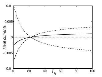
Figure 1: The heat currents $\dot{Q}_{\mu}[J/s]$ versus $T_{H}[K]$ in weak coupling regime. The solid line, the dashed line and the dash-dotted line correspond to $\dot{Q}_{C}$, $\dot{Q}_{H}$ and $\dot{Q}_{R}$, respectively. Here $g=0.001\omega_{H}$. In particular, we set $\gamma=0.001\omega_{H}$ throughout the paper.

III Results and discussions

In order to study the thermodynamical behavior of the stationary state, we will find the stationary-state solution $\rho^{S}$ of the master equation given by Eq. (18). To do so, we let $\rho^{S}$ have the vanishing derivative on $t$, i.e.,

$$\dot{\rho}^{S}=0.$$ (23)

Thus we will arrive at the following equations

$$M\left|\rho\right\rangle = 0,$$ (24)

$$\rho_{ij}^{S} = 0,i\neq j,$$ (25)

where $\left|\rho\right\rangle=[\rho_{11}^{S},\rho_{22}^{S},\rho_{33}^{S},\rho_{44}^{S},\rho_{55}^{S},\rho_{66}^{S},\rho_{77}^{S},\rho_{88}^{S}]^{T}$ is the vector made up of the diagonal entries of the stationary density matrix $\rho^{S}$, and

$$M=\sum\limits_{\mu=1}^{3}M_{\mu}.$$ (26)

In order to give the explicit expression for $M_{\mu}$, we first define some new quantities $m_{ij},i,j=1,2,3$ as

$$m_{11} = 2\mathbf{J}_{11}\otimes\left(\mathbf{1}_{+}\otimes\mathbf{1}_{+}+\mathbf{1}_{-}\otimes\mathbf{1}_{-}\right),$$ (27)

$$m_{12} = \mathbf{1}\otimes C_{23}\left(\mathbf{J}_{12}\otimes\mathbf{1}_{-}\right)C_{23}^{{\dagger}},$$ (28)

$$m_{13} = \mathbf{J}_{13}\otimes\left(\mathbf{1}_{+}\otimes\mathbf{1}_{-}+\mathbf{1}_{-}\otimes\mathbf{1}_{+}\right),$$ (29)

$$m_{21} = \left(\mathbf{1}_{+}\otimes\mathbf{J}_{21}\otimes\mathbf{1}_{+}+\mathbf{1}_{-}\otimes\mathbf{J}_{21}\otimes\mathbf{1}_{-}\right),$$ (30)

$$m_{22} = 2\left(\mathbf{1}_{+}\otimes\mathbf{J}_{22}\otimes\mathbf{1}_{-}+\mathbf{1}_{-}\otimes\mathbf{J}_{22}\otimes\mathbf{1}_{+}\right),$$ (31)

$$m_{23} = C_{13}\left(\mathbf{J}_{23}\otimes\mathbf{1}\otimes\mathbf{1}_{+}\right)C_{13}^{\dagger},$$ (32)

$$m_{31} = C_{21}\left(\mathbf{1}_{-}\otimes\mathbf{J}_{31}\otimes\mathbf{1}\right)C_{21}^{\dagger},$$ (33)

$$m_{32} = \left(\mathbf{1}_{+}\otimes\mathbf{1}_{-}+\mathbf{1}_{-}\otimes\mathbf{1}_{+}\right)\otimes\mathbf{J}_{32},$$ (34)

$$m_{33} = 2\left(\mathbf{1}_{+}\otimes\mathbf{1}_{+}+\mathbf{1}_{-}\otimes\mathbf{1}_{-}\right)\otimes\mathbf{J}_{33},$$ (35)

where

$$\mathbf{1=}\left(\begin{array}[]{cc}1&0\\ 0&1\end{array}\right),\mathbf{1}_{\pm}\mathbf{=}\frac{\mathbf{1}\pm\sigma_{z}}{2}$$ (36)

and $C_{jk},j,k=1,2,3$ denotes the control-not gate with $j$ standing for the control qubit and $k$ representing the target qubit. For example,

$$C_{12}=\left(\mathbf{1}\oplus\sigma_{x}\right)\otimes\mathbf{1}.$$ (37)

In addition, $\mathbf{J}_{\mu j}$ in Eqs. (27-35) is a matrix with its entries corresponding to the spectral density. It can be explicitly represented by

$$\mathbf{J}_{\mu j}=\left(\begin{array}[]{cc}-J_{\mu}\left(-w_{\mu j}\right)&J_{\mu}\left(w_{\mu j}\right)\\ J_{\mu}\left(-w_{\mu j}\right)&-J_{\mu}\left(w_{\mu j}\right)\end{array}\right).$$ (38)

Based on Eqs. (27-35), $M_{\mu}$ can be explicitly written by

$$M_{\mu}=\sum_{j}m_{\mu j}.$$ (39)

$M_{\mu}$ apparently includes three terms which are related to three atoms respectively. Using the definition of the heat current [34,36], we can find that the heat current subject to $\mu$th reservoir reads

$$\dot{Q}_{\mu}=Tr\left\{H_{S}\mathcal{L}_{\mu}\text{[}\rho^{S}\text{]}\right\}=\left\langle\epsilon\right|M_{\mu}\left|\rho\right\rangle.$$ (40)

It is obvious that $\dot{Q}_{\mu}$ corresponding to $M_{\mu}$ is uniquely determined by the steady state $\left|\rho\right\rangle$. It is fortunate that $\dot{Q}_{\mu}$ can be explicitly calculated, because Eq. (23) can be analytically solved. However, the concrete form of $\left|\rho\right\rangle$ is so tedious that we cannot write it here. Therefore, in the following part, we will have to give a numerical analysis based on the analytical $\left|\rho\right\rangle$ (even though it is not given here).

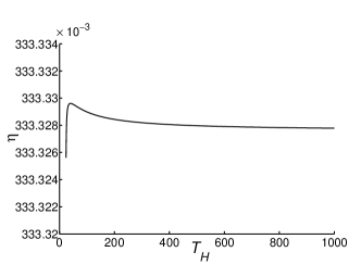
Figure 2: The efficiency $\eta$ of the refrigerator versus $T_{H}[K]$ in the weak coupling regime. The efficiency changes slightly and it can be considered to be almost invariant within a good approximation, which can also be supported by Fig. 5.

At first, we would like to consider the weak coupling case, i.e., $g\sim\gamma_{\mu}$. Based on Eq. (40), we plot the heat currents in Fig. 1. Here we suppose $\omega_{H}=3$ and $\omega_{C}=1$, so $\omega_{R}=4$. In addition, we let the room temperature be $21K$ and the temperature of the cold reservoir be $18K$ (Of course, if the other parameters are chosen, one will get the similar results). When the temperature of the hot reservoir is low, the heat will flow into the cold reservoir. So the cold atom $C$ is heated. However, with the temperature of the hot reservoir increasing, one can find that all the heat currents will become zero simultaneously when $T_{H}=T_{v}=\frac{\omega_{H}}{\frac{\omega_{R}}{T_{R}}-\frac{\omega_{C}}{T_{C}}}\simeq 22.24K$ (so long as the coupling $g$ and the decay rate $\gamma$ are small enough.). This virtual temperature $T_{v}$ is just consistent with Ref. [32] which is closely related to Ref. [28]. In addition, one can also see that the heat currents are increasing with the increase of $T_{H}$. That is, the thermodynamic machine works as a refrigerator. An obvious feature is that the heat currents subject to the hot reservoir and the cold reservoir have the same direction (sign) and the sign is determined by the virtual temperature $T_{v}$. However, if $\frac{\omega_{R}}{T_{R}}=\frac{\omega_{C}}{T_{C}}$, one will find that no matter how large $T_{H}$ is, $\dot{Q}_{C}$ is always less than zero. In addition, we also consider the efficiency of the quantum refrigerator, which is illustrated in Fig. 2. Here the efficiency $\eta$ is defined by $\eta=\frac{\dot{Q}_{C}}{\dot{Q}_{H}}$ which was deeply studied in Ref. [30]. In a simple way, it can be understood as that, by extracting heat (current) $\dot{Q}_{H}$ from the hot reservoir, we are able to extract heat (current) $\dot{Q}_{C}$ from the cold reservoir whilst dumping heat (flow) $\dot{Q}_{R}$ into the reservoir $R$. It was also shown that $\eta$ for the self-contained refrigerator in Ref. [28] was given by $\frac{\omega_{C}}{\omega_{H}}$. Take the current parameters into account, it should be $\eta=\frac{1}{3}$. From our Fig. 2, at the first glance, the efficiency seems to have a peak somewhere. But one can further find that to some acceptable approximation, $\eta$ can be considered to be invariant on $T_{H}$ and just equal to $\frac{1}{3}$. The peak will be explained in the next part. All these show that in the weak coupling regime, the treatment with respect to the quantum optical master equation (QOME) has the well consistency with the previous results given in Ref. [28]. This implies that the QOME could not be sensitive to the rotating wave approximation corresponding $g>>\gamma_{\mu}$ in this case, which could lead to that the QOME is valid here.

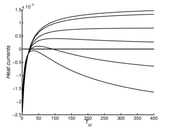
Figure 3: The heat currents $\dot{Q}_{C}[J/s]$ versus $T_{H}[K]$ for different coupling constants. From the top to the bottom, $g=0.001\omega_{H},0.1\omega_{H},0.2\omega_{H},0.25\omega_{H},0.3\omega_{H},0.35\omega_{H}$. The straight line means zero heat current.

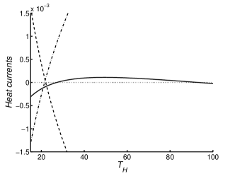
Figure 4: The heat currents versus $T_{H}[J/s]$ in the strong coupling regime. Here $g=0.3\omega_{H}$ and $\gamma=0.001\omega_{H}$. The dotted line corresponds to the zero heat current and the other lines denote the same heat currents as Fig. 1. $\dot{Q}_{C}$ is first pushed to the positive direction and then is suppressed back to the negative direction.

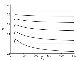
Figure 5: The efficiency $\eta$ versus $T_{H}[K]$ with different coupling constants. The lower straight line corresponds to the zero efficiency. From the top to the bottom, the lines correspond to $g=0.001\omega_{H},0.1\omega_{H},0.15\omega_{H},0.2\omega_{H},0.25\omega_{H},0.3\omega_{H}$. In particular, $\eta=const.$ within acceptable approximations for $g=0.001\omega_{H}$, which is consistent to Fig. 2.

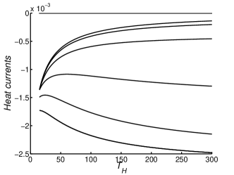
Figure 6: The heat currents $\dot{Q}_{C}[J/s]$ versus $T_{H}[K]$ for different coupling constants. Here we let $T_{C}=10K$ and $T_{R}=40K$ in order to satisfy $\frac{\omega_{C}}{T_{C}}=\frac{\omega_{R}}{T_{R}}=\frac{1}{10}$. The upper straight line means zero heat current. From up to down, the lines correspond to $g=0.001\omega_{H},0.1\omega_{H},0.2\omega_{H},0.3\omega_{H},0.4\omega_{H},0.5\omega_{H}$, respectively.

Now let’s turn to our main results i.e., $g>>\gamma_{\mu}$. To find the influence of the coupling strength $g$, we keep $\omega_{\mu}$ and $\gamma_{\mu}$ invariant and plot the heat currents in Fig. 3 with different $g$. One will immediately see that the large $g$ directly leads to the suppression of the heat current $\dot{Q}_{C}$. Compared with the case of weak coupling, the high temperature $T_{H}$ could have the negative role in the cooling of the cold atom. It is obvious that the atom C cannot be cooled if the coupling strength $g$ is too large, which is opposite to the case of weak internal coupling regime. In particular, given $T_{C}$, $T_{R}$ and all the frequencies, one will see that the cooling only happens within some range of $T_{H}$, which has also been shown in Fig. 4. Thus the direct conclusion is that the strong coupling is not beneficial to the cooling from the point of refrigerator of view. In addition, one can also find that the heat currents don’t meet at a single point (temperature), which is quite different from the weak coupling case. The heat currents don’t change their direction simultaneously. In particular, the heat current $\dot{Q}_{C}$ seems not to be directly relevant to the virtual temperature $T_{v}$. The machine becomes a refrigerator only when $\dot{Q}_{C}>0$ where one will find $T_{H}\simeq 27.25K\neq 22.24K=T_{v}$. As a refrigerator, the efficiency depends on the coupling constant $g$. The numerical results are given in Fig. 5. It is shown that the efficiency will become larger if $g$ becomes less. It will arrive at a constant efficiency ($\eta=\frac{\dot{Q}_{C}}{\dot{Q}_{H}}=\frac{\omega_{C}}{\omega_{H}}=\frac{1}{3}$) when it reaches the weak coupling limit. However, the efficiency will change with $T_{H}$ if it is still in the case of strong coupling. The peak of the efficiency mainly results from the suppression of cooling induced by the strong coupling. In particular, the suppression becomes strong for large $T_{H}$. When the reservoir $H$ is hot enough, the reservoir could be heated instead of cooled, which can be obviously found for $g=0.3\omega_{H}$. When the internal coupling become weak, the suppression will be weakened. If it is weak enough, the suppression won’t be so apparent that the peak can be neglected to some good approximation, which is just illustrated in Fig. 2. When $\frac{\omega_{R}}{T_{R}}=\frac{\omega_{C}}{T_{C}}$, one can also find that no matter what the coupling constant is, it is impossible to make a refrigerator. However, from a different angle, we can find that in the weak coupling limit, $\dot{Q}_{C}$ is reduced if we increase $T_{H}$. On the contrary, when the coupling is strong, $\dot{Q}_{C}$ become large with $T_{H}$ increasing. This is shown in Fig. 6.

IV Conclusions

In summary, we have revisited the self-contained refrigerator in the strong internal coupling regime by employing the quantum optical master equation. We find that the strong internal coupling reduces the cooling ability. In particular, in this regime, the considered machine demonstrates quite different (and even converse) thermodynamic behaviors compared with that in Ref. [28]. In addition, we find that the quantum optical master equation provides the consistent results with the Ref. [28] in the weak internal coupling regime, even though the rotating wave approximation, in principle, does not allow the weak internal coupling. This could shed new light on the validity of the master equation.

This work was supported by the National Natural Science Foundation of China, under Grant No.11375036 and 11175033, and the Xinghai Scholar Cultivation Plan.

References

• (1) S. Carnot, Réflexions sur la Puissance Motrice du Feu (Bachelier Libraire, Paris, 1824).
• (2) G. Gemma, M. Michel and G. Mahler, Quantum Thermodynamics, Springer (2004).
• (3) E. P. Gyftopoulos and G. P. Beretta, Thermodynamics: Foundations and Appications, Dover (2005).
• (4) A. E. Allahverdyan, R. Ballian and Th. M. Nieuwenhuizen, J. Mod. Opt. 51, 2703 (2004).
• (5) F. Tonner and G. Mahler, Phys. Rev. E 72, 066118 (2005).
• (6) M. Henrich, M. Michel and G. Mahler, Europhys. Lett. 76, 1057 (2006).
• (7) M. Youssef, Mahler and A.-S. F. Obada, Phys. Rev. E 80, 061129 (2009).
• (8) M. Henrich, G. Mahler and M. Michel, Phys. Rev. E 75, 051118 (2007).
• (9) A. E. Allehverdyan and Th. M. Nieuwenhuizen, Phys. Rev. Lett. 85, 1799 (2000).
• (10) T. D. Kien, Phys. Rev. Lett. 93, 140403 (2004).
• (11) T. E. Humphrey and H. Linke, Physica E 29, 390 (2005).
• (12) D. Janzing et al., Int. J. Th. Phys. 39, 2717 (2000).
• (13) J. Geusic, E. S. du Bois, R. D. Grasse, and H. Scovil, J. Appl. Phys. 30, 1113 (1959).
• (14) H. Scovil and E. S. du Bois, Phys. Rev. Lett. 2, 262 (1959).
• (15) J. Geusic, E. S. du Bois, and H. Scovil, Phys. Rev. 156, 343 (1967).
• (16) R. D. Levine and O. Kafri, Chem. Phys. Lett. 27, 175 (1974).
• (17) A. Ben-Shaul and R. D. Levine, J. Non-Equilib. Thermodyn. 4, 363 (1979).
• (18) D. Segal and A. Nitzan, Phys. Rev. E 73, 026109 (2006).
• (19) E. Geva and R. Kosloff, J. Chem. Phys. 96, 3054 (1992).
• (20) E. Geva and R. kosloff, J. Chem. Phys. 104, 7681 (1996).
• (21) T. Feldmann and R. Kosloff, Phys. Rev. E 61, 4774 (2000).
• (22) J. P. Palao, R. Kosloff and J. M. Gordon, Phys. Rev. E 64, 056130 (2001).
• (23) R. Kosloff and T. Feldmann, Phys. Rev. E 82, 011134 (2010).
• (24) T. Feldmann, E. Geva and P. Salamon, Am. J. Phys. 64, 485 (1996).
• (25) T. Feldmann and R. Kosloff, Phys, Rev. E 68, 016101 (2003).
• (26) H. T. Quan et al., Phys. Rev. E 76, 031105 (2007).
• (27) T. E. Humphrey, R. Newbury, R. P. Taylor and H. Linke, Phys. Rev. Lett. 89, 116801 (2002).
• (28) N. Linden, S. Popescu and P. Skrzypczyk, Phys. Rev. Lett. 105, 130401 (2010).
• (29) N. Linden, S. Popescu and P. Skrzypczyk, arXiv: 1010.6029v1 [quant-ph].
• (30) P. Skrzypczyk, N. Brunner, N. Linden and S. Popescu, J. Phys. A: Math. Theor. 44, 492002 (2011).
• (31) S. Popescu, arXiv: 1009.2536v1 [quant-ph].
• (32) N. Brunner, N. Linden, S. Popescu, P. Skrzypczyk, Phys. Rev. E 85, 05111 (2012).
• (33) D. F. Walls, G. J. Milburn, Quantum Optics (Springer-Verlag, Berlin Heidelberg, 1994).
• (34) H. P. Breuer and F. Petruccione, The Theory of Open Quantum Systems (Oxford University Press, Oxford, U. K., 2002).
• (35) C. Majenz, T. Albash, H.-P. Breuer, and D. A. Lidar, Phys. Rev. A 88, 012103 (2013).
• (36) T. M. Nieuwenhuizen and A. E. Allahverdyan, Phys. Rev. E 66, 036102 (2002).