On the Spin of the Black Hole in IC 10 X-1

Abstract

The compact X-ray source in the eclipsing X-ray binary IC 10 X-1 has reigned for years as ostensibly the most massive stellar-mass black hole, with a mass estimated to be about twice that of its closest rival. However, striking results presented recently by Laycock et al. reveal that the mass estimate, based on emission-line velocities, is unreliable and that the mass of the X-ray source is essentially unconstrained. Using Chandra and NuSTAR data, we rule against a neutron-star model and conclude that IC 10 X-1 contains a black hole. The eclipse duration of IC 10 X–1 is shorter and its depth shallower at higher energies, an effect consistent with the X-ray emission being obscured during eclipse by a Compton-thick core of a dense wind. The spectrum is strongly disk-dominated, which allows us to constrain the spin of the black hole via X-ray continuum fitting. Three other wind-fed black-hole systems are known; the masses and spins of their black holes are high: $M\sim 10-15{\rm M}_{\odot}$ and $a_{*}>0.8$. If the mass of IC 10 X-1’s black hole is comparable, then its spin is likewise high.

1 Introduction

IC 10 X–1, a luminous and variable X-ray binary in the dwarf irregular galaxy IC 10, was discovered by Brandt et al. (1997) using ROSAT. IC 10 is notable for being the closest starburst galaxy, at a distance of $750\pm 50$ kpc (Demers et al., 2004; Vacca et al., 2007; Sanna et al., 2008; Kniazev et al., 2008; Kim et al., 2009), and for its marked overabundance of massive stars. In particular, there is a large population of Wolf-Rayet (W-R) stars, despite IC 10 being extremely metal poor (e.g., Sakai et al., 1999; Wang et al., 2005, and references therein). IC 10 X–1 contains one such massive W-R star that closely orbits the compact X-ray source [MAC92] 17A (Clark & Crowther, 2004), which we also refer to as IC 10 X–1. Like a number of other X-ray binary systems (e.g., Cyg X–1, Gallo et al. 2005; LMC X–1, Pakull & Angebault 1986; SS 433,Fabrika 2004, XTE J1550–564, Steiner & McClintock 2012; Wang et al. 2003; Cyg X–3, Sánchez-Sutil et al. 2008; GRS 1915+105 and GRO J1655–40, Heinz 2002), IC 10 X–1 is embedded in a low-density bubble, $\sim 150$ pc across, and it is radio bright (Yang & Skillman, 1993; Bauer & Brandt, 2004; Wang et al., 2005). The X-ray source exhibits a low-frequency 7 mHz quasi-periodic oscillation (Pasham et al., 2013). Based on the brightness of the source, in their discovery paper Brandt et al. (1997) suggested IC 10 X–1 as a likely black hole W-R binary.

One intriguing outcome of the present census of stellar-black hole spin measurements is a possible dichotomy between the wind-fed (“X-ray persistent”) systems as compared to the Roche-lobe overflow (“X-ray transient”) systems (see McClintock et al. 2014; Steiner et al. 2014): The transients have spins that range widely, from near-zero to near-maximal; recent evidence suggests that much or all of the spin in these systems may have been supplied through long-acting accretion torques spinning up an initially non-rotating black hole (Fragos & McClintock, 2015). In contrast, the three known wind-fed systems – Cyg X–1, LMC X–1, and M33 X–7 – harbor high-spin black holes ($a_{*}>0.8$). The high spins of the wind-fed systems are especially noteworthy given the young ages of these systems, which precludes appreciable spin-up through accretion torques, implying that the spins of these black holes were imparted during the process of their formation. Another distinction between the two classes of X-ray binaries is that the black holes in the wind-fed systems are significantly more massive. Among the three established wind-fed systems, M33 X–7, which has a massive ($M_{2}\approx 70{\rm M}_{\odot}$) O-star companion (Orosz et al., 2007), is similar to IC 10 X–1 in that it is located in a low-metallicity Local Group galaxy at a distance of $\sim 800$ kpc and contains a quite massive $\sim 15{\rm M}_{\odot}$ black hole primary.

Firm dynamical estimates of the masses of two-dozen black holes (BHs) in X-ray binaries have been obtained, almost exclusively by measuring the Doppler shifts of photospheric absorption lines. Up until eight years ago, the distribution of masses was relatively narrow, $6{\rm M}_{\odot}$–$15{\rm M}_{\odot}$, a result that was upended by startling evidence, based on He II emission-line velocities, that IC 10 X–1 is comprised of a $\gtrsim 30{\rm M}_{\odot}$ BH in a tight 35-hr orbit with a comparably massive $\sim 35{\rm M}_{\odot}$ W-R secondary (Prestwich et al., 2007; Silverman & Filippenko, 2008). Modeling the evolutionary history of this extraordinary system proved to be quite a challenge (e.g., Bogomazov 2014). Very recently, however, the mass estimate for IC 10 X-1 has been shown to be invalid: Laycock et al. (2015a) demonstrated that the He II line does not originate from the star, but rather from a shadowed region in the wind of the W-R companion. They conclude that the mass of the primary is currently unknown and in Laycock et al. (2015b) that it may even be consistent with the mass of a neutron star.

The spins of stellar-mass BHs are presently being measured using two X-ray spectroscopic techniques: continuum-fitting and reflection modeling. Spin is a quantity of great interest because according to the “no-hair theorem” spin and mass together uniquely and fully characterize a BH in general relativity. Both methods rely upon a single foundational assumption, namely that the inner-disk terminates at the innermost stable circular orbit (ISCO). Observations establish the presence of a constant inner radius in BH systems in certain states (e.g., Steiner et al. 2010). Meanwhile, theoretical studies have identified this constant radius with the ISCO (e.g., Zhu et al. 2012; Kulkarni et al. 2011; Noble et al. 2010, but see Noble et al. 2009).

In the X-ray continuum-fitting method, one models the thermal emission from the multi-temperature accretion disk to constrain the size of the ISCO radius; the method requires accurate measurements of the BH’s mass $M$, the system’s inclination $i$ and distance $D$. For the reflection method, one models the relativistic distortion of fluorescent features from an accretion disk that is illuminated by a coronal source, with a focus on the $\sim 6.7$ keV Fe K line. The extended red wing is a measure of the strength of the gravitational potential and allows one to estimate the disk’s inner radius. To date, application of these methods has yielded estimates of spin for a total of $\sim 20$ stellar BHs (Reynolds 2014; McClintock et al. 2014; Steiner et al. 2014, and references therein); additionally, the spins of a comparable number of supermassive BHs have been measured via reflection modeling (see e.g., Walton et al. 2012; Risaliti et al. 2013; Brenneman 2013).

Given that the mass of the compact X-ray source is now unknown, we examine afresh the case of IC 10 X–1. We begin by considering the possibility that the X-ray source is a neutron star (NS) and show that this model is improbable. Having concluded that IC 10 X–1 contains a BH primary, we use the continuum-fitting method and an unrivaled spectrum obtained in simultaneous observations made using Chandra and NuSTAR  to place constraints on the spin of the BH.

2 Data

We carried out a joint observation using Chandra and NuSTAR for $\sim 150$ ks – just over one full orbit – starting on UT 2014 November 6. Chandra was operated using a single chip, ACIS I-3, using a 100-row sub-array in order to minimize photon pileup, which causes distortion of the spectrum. This operating mode reduced the frame-time nearly tenfold, to just 0.4 s. Because the maximum count rate in ACIS was merely  0.2 s^-1 (corresponding to an isotropic luminosity of $\sim 1.2\times 10^{38}$ erg s^-1), the resulting degree of photon pileup is minimal, $\sim 1\%$. The quite minor impact of the remaining pileup is nevertheless accounted for in all spectral fits, using the pileup model of Davis (2001). Because the pileup was so modest, we could not fit for the model’s grade migration term, and merely kept it fixed at a fiducial value of $0.7$. This and other pileup settings had no impact on our fit results, but were incorporated for completeness in the analysis.

Chandra data have been reduced using ciao v4.7. Because the data were obtained near the chip edge, the response files are calibrated using an exposure map and aperture correction, which has modest ($\sim 1\%$) impact on the effective area. Our final spectrum employs a circular aperture with a 5 arcsec radius centered on IC 10 X–1, which was near the detector aim Obpoint. The background is obtained using a blank region from the same observation. Data have been binned to adequately oversample the detector resolution (by a factor $\sim 3$), and to a minimum of one count per bin. Chandra spectra are fitted over 0.3–9 keV (IC 10 X–1 produces insignificant signal above this range for Chandra), and NuSTAR from 3–30 keV. All data were standardized to the Toor & Seward (1974) spectral standard model of the Crab using the model crabcor following Steiner et al. (2010). This corresponds to a shift in spectral slope of $\Delta\Gamma=0.02$ for Chandra and a renormalization of $f=1.11$. With NuSTAR, $\Delta\Gamma=0.00$ (Madsen et al., 2015), and a floating cross-normalization term was fitted.

We reduced the NuSTAR data using the standard pipeline, nupipeline, part of the NuSTAR Data Analysis Software (nustardas, v1.4.1), with the latest instrumental calibration files (caldb v20150316). The unfiltered event files were cleaned with the standard depth correction, which significantly reduces the internal high-energy background, and passages through the South Atlantic Anomaly were removed. Source spectra and instrumental responses were produced for each of the two focal plane modules (FPMA/B) using nuproducts, extracted from a circular region of radius 50^′′ centered on IC 10 X–1. The background was estimated from a much larger region on the same detector as the source. In order to maximize the good exposure, in addition to the standard “science” (mode 1) data, we also extracted the available “spacecraft science” (mode 6) data. These are events collected while the source is still visible to the X-ray optics, but the star tracker located on the optics bench no longer gives a valid solution, so the aspect solution is constructed from the star trackers on the spacecraft bus instead. This typically results in some reduction in image reconstruction capabilities, but not in the spectral response of the instruments (see Walton et al. and Fuerst et al., in preparation, for more details). In this case, the source point-spread function (PSF) degradation was very mild, and so the reduction of the mode 6 data simply followed the standard procedure outlined above, with a slightly larger source region of radius 55^′′ adopted to account for this slight degradation. These data provided an additional $\sim$30% exposure for this observation. Finally, owing to the low signal-to-noise, we combined the data from FPMA and FPMB using addascaspec. The resulting NuSTAR spectrum provides a detection up to $\sim$30 keV.

IC 10 X–1 is in a fairly isolated field. The closest field source is $1.0\arcmin$ from IC 10 X–1, and is only 1% as bright. Meanwhile, the brightest source in the FOV is $<7$% as bright and is $1.6\arcmin$ from IC 10 X–1. Neither source was problematic for the NuSTAR observations. We note, however, that the NuSTAR data appear to imply surprisingly lower flux than Chandra. The data are fainter than would be expected by $\sim 20\%$. In effort to understand this, we consider sources of calibration uncertainty in the NuSTAR data. By comparing the NuSTAR point spread enclosed energy function of IC 10 X–1 to that of the model used for correcting the PSF in the NuSTAR pipeline, we estimate that the actual count rate might be off by as much as 10–15%. In addition, IC 10 X–1 is located close to a detector edge, which at times sweeps through the PSF. This is accounted for in the pipeline, but the correction is not accurate, particularly at low count rates. While difficult to precisely assess, a conservative 5-10% uncertainty is likely from this. Finally, we note that the NuSTAR flux can be off globally by $\pm 5\%$ (Madsen et al., 2015). Therefore, in total, the net error on NuSTAR fluxes may be up to $\sim 25\%$.

Spectral analysis was conducted using xspec v.12.9.0c (Arnaud, 1996), and model optimization employed xspec’s c-statistic (“$C^{2}$”) (Cash, 1979), as appropriate for Poisson-distributed data.

The Chandra and NuSTAR light curves from our observation are shown in Figure 1. The strong dip marks the passage of the X-ray primary source behind a thick, wind-obscured core of the W-R star, marked by energy-dependent scattering (e.g., Orosz et al. 2007; Barnard et al. 2014). We select in- and out-of eclipse regions (“low” and “high”, respectively). The high-flux region is split into two segments (“high-1” and “high-2”), to check for possible phase variation as the source passes through the strong wind of the companion.

3 Wind and Absorption

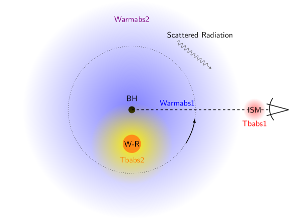
Figure 2: A schematic of the BH – W-R system illustrating the various wind and warm absorber components.

The broadband X-ray flux in eclipse is just $\sim$12% of the flux out of eclipse. Given the presence of a powerful W-R wind in which the source is embedded, the origin of this emission is likely to be electron scattering of X-rays from the photoionized wind of the W-R star and we adopt this scenario in using a corresponding model for which this signal is attributed to the inner-region’s X-ray emission scattering off of an extended “halo” of electrons in the wind. A schematic of this system is shown in Figure 2. As pointed out, e.g., by Barnard et al. (2014), this is no true “eclipse” in the sense of a solid body obscuring another, but rather must be attributed to a Compton-thick scattering agent, which is sensibly depicted by Laycock et al. (2015a) as a thick shell of wind surrounding the star. This picture is similarly compatible with the parallel system NGC 300 X–1, a 33 hr orbit WR-BH binary (Binder et al., 2015). We therefore additionally allow for highly absorbed emission from the primary source passing through such a Compton thick wind (the scattered contribution is present in both the low and high phases); for the first time, the high-energy coverage provided by NuSTAR allows for the detection of the transmitted photons at high energies which are insensitive to the veiling of the large gas column (as well as the Compton component). Ideally, this model would allow for the absorption to vary with phase over the full duration of the eclipse. However, given the faintness of the source to both instruments, we make a simplification and require a single, characteristic column of absorber to capture this effect in the “low” observation. We note, however, that given sufficient signal in conjunction with a more complete model of the W-R companion and an expected wind profile, one could place a firm constraint on the inclination using the phase evolution of the column. Our data is not of this quality, and such an investigation is beyond the scope of this paper.

A strong and broad absorption signature is detected with Chandra near $\sim 2\leavevmode\nobreak\ {\rm keV}$. The most obvious origin for such a feature is absorption in the powerful ionized winds. We delve into the absorption features further in Section 4.2. To model this appropriately, we have employed the photoionization code xstar (Kallman & Bautista, 2001) assuming the gas is hydrogen depleted (for practical reasons, we ran the code using a hydrogen abundance of 0.1 solar), and metal poor (each metal set to 0.15 solar abundance), with a solar setting for He. We employed as an input spectrum, the average spectrum corresponding to the out-of-eclipse model, with neutral absorption removed. We computed a table of warm absorbers corresponding to a range of columns and ionizations widely bracketing our system, spanning a range in column density of $2\times 10^{20}-2\times 10^{24}$ cm^-2 and of log $\xi=0-4$. (We assume a covering fraction of unity for the warm absorber.) This gas is ascribed a turbulent velocity (free in the fit) using a Gaussian smearing kernel in the same manner as Gierliński & Done (2004). Here, such blurring is ad-hoc; it may, for instance, be indicative of a mixture of ionizations given the multi-phased ionization structures present in the wind (see Laycock et al. 2015b, and Vilhu et al. 2009). The warm absorber’s ionization is fitted for and tied across phases, but the gas column is allowed to vary between “low” and each of the “high” phases. Because the 2 keV feature was not completely removed using this model, we also included a Gaussian absorption line that significantly improved the spectral fit ($\Delta C^{2}/\Delta\nu=45.5/3$), and produced relatively minor influence on the other fit parameters.

Figure 1: Chandra and NuSTAR (FPMA+FPMB) background-subtracted light curves of IC 10 X–1. As a guide to the eye, a running third-order polynomial fit is shown in red over the Chandra data. The out-of-eclipse (“high-1” and “high-2”) and in-eclipse (“low”) intervals from the text are indicated. The impressive duration of the eclipse phase, $\sim 30$% of an orbital cycle, is a consequence of the dense and powerful stellar winds emanating from the W-R companion. In the lower-panel, the Chandra curve is overlaid for reference, having been simply rescaled (red dashed). A running fit to the NuSTAR data is in blue. Note that the eclipse appears both shallower and also somewhat narrower in NuSTAR compared to Chandra. This is a direct result of NuSTAR’s sensitivity to higher energies, which are less affected by absorption in the wind.

4 Results

We first consider models in which the compact primary of IC 10 X–1 is an accreting neutron star with its spectrum dominated by a thermal component of radiation from the star’s photosphere. We show that the model implies stellar radii that are much greater than those observed for luminous accreting neutron stars, and we therefore discard this model and consider the one viable alternative, namely, that the compact object is a black hole. Using the continuum-fitting method, while considering liberal ranges for the mass of the black hole and disk inclination, we show that the black hole is spinning rapidly.

4.1 A Neutron Star Considered

Accreting NS systems in low-mass X-ray binaries fall into two categories: “Z” and “atoll”, the names of which refer to the characteristic shape traced out by each in an X-ray hardness–intensity diagram. Between the two classes, Z-sources are the most luminous, generally emitting near, even above, the Eddington limit ($L\sim 0.5\leavevmode\nobreak\ L_{\rm Edd}$ and upwards; Homan et al. 2010).

The observed (isotropic-equivalent) source luminosity in the Chandra band is $1.5\times 10^{38}$ erg s^-1 (0.5–10 keV), or $\approx 85$% of the Eddington luminosity (adopting $L_{\rm Edd}=1.25\times 10^{38}\times M/{\rm M}_{\odot}$ erg s^-1 and $M=1.4\leavevmode\nobreak\ {\rm M}_{\odot}$). This luminosity is squarely in the range observed for Z sources. That the spectrum of IC 10 X–1 is predominately thermal is indicated by the much lower luminosity observed by NuSTAR above 10 keV, which is $\lesssim 5$% of the luminosity in the full Chandra band. Meanwhile, the difference between the observed luminosity and the intrinsic source luminosity due to scattering in the stellar wind (Section 3) is $\lesssim 10$% and unimportant for the discussion at hand. Additional evidence that the spectrum is thermal is provided by results presented in this section; namely, in fitting the spectrum with thermal models, we find that the power-law component is exceptionally faint and can be accounted for by upscattering of at most only a few percent of the seed photons.

Before presenting our analysis of the spectrum of IC 10 X–1, we discuss pertinent results for accreting neutron stars with a focus on estimates of their radii. The key neutron star binary for our discussion is XTE J1701–462. This remarkable source traced out the full-repertoire of Z source states and then transitioned through a lower-luminosity atoll phase (Homan et al., 2007). In studying the evolution of the source, Lin et al. (2009b) (hereafter L09) employed a model comprised of three spectral components: (i) a single-temperature blackbody from the stellar surface, which describes emission from the boundary layer (sometimes called a “spreading” layer); (ii) a cooler multi-temperature blackbody from an accretion disk; and (iii) a power-law component due to Compton up-scattering.

We note that the model of the boundary layer region is relatively uncertain. It is frequently assumed to be optically thick and of modest height, of order $\lesssim 1$ km, (e.g., Inogamov & Sunyaev 1999; Revnivtsev & Gilfanov 2006). Alternatively, the boundary layer has been modeled as a hot, low-density gas that at high luminosities can extend both radially and out of the disk plane by more than 1 stellar radius, in which case it would behave like a scattering atmosphere (akin to a corona; Popham & Sunyaev 2001).

Given the theoretical uncertainties in the size of the boundary layer, we turn to empirical evidence that shows it is compact. For our touchstone source XTE J1701–462, during its evolution as a Z source its power-law component was generally negligible and its blackbody radius was in the range $\approx 2-4$ km over the luminosity range $\sim 0.5-2\leavevmode\nobreak\ L_{\rm Edd}$. In evolving through the fainter atoll phase in soft states, the blackbody radius remained constant at 1.7 km. In every observation throughout the outburst, the radius was strictly $<6$ km; such estimates are firm because the distance estimate for XTE J1701–462 is based on super-Eddington type I bursts (Lin et al., 2009a).

Meanwhile, small radii are widely reported in studies of other luminous accreting NSs. For the Z source GX 17+2, Lin et al. (2012) found that across all states the blackbody radius was $<6$ km. In a study of six canonical Z sources, Church et al. (2012) found blackbody radii that are consistently $\lesssim 10$ km (apart from the unstable “flaring branch” for which the maximum radius observed was 16 km). While Z sources are most appropriate for comparison with IC 10 X–1, we note that radius estimates reported for the less luminous atoll sources are typically $\sim 2$ km (Lin et al. 2007, 2010; Barret & Olive 2002, and references therein) and are strictly $<8$ km in the works cited. The small blackbody radii inferred for XTE J1701–462 and other NSs constitutes the strongest empirical evidence for a compact NS boundary layer.

We now present the results of our analysis of the data for IC 10 X–1 with a focus on the blackbody radius of its hypothetical neutron star. Our analysis follows closely the lead of L09. Our spectral model allows for the modest effects due to the presence of the phase-dependent warm absorber described in Section 3 and to scattered light, using the in-eclipse spectrum to calibrate the magnitude of its contribution. We consider two basic models: Model 1 is a single-temperature blackbody; Model 2 is this same blackbody component plus an accretion disk component (modeled via ezdiskbb; Zimmerman et al. 2005).

For both models, we: (1) model Compton scattering of thermal photons in a corona using simpl (Steiner et al., 2009). The photon spectral index is poorly determined, and so we fix $\Gamma=2$, a choice that is in this case inconsequential for the determination of the blackbody radius. (2) We include neutral absorption using tbabs (with wilm abundances; Wilms et al. 2000, and vern cross-sections; Verner et al. 1996). (3) Initially, we model the $\sim 2$ keV absorption feature (Section 3) with a Gaussian. This component turns out to be significant only for Model 1, and so we omit it in our final analysis for Model 2.

Results for the two models are summarized in Table 1. The data are well-fitted by both Models 1 and 2 with $C^{2}/\nu=1.01$ and 0.96, respectively. As mentioned above, the Compton component is faint, as measured by the parameter $f_{\rm sc}$ in Table 1; only a few percent of the thermal photons are scattered into the power law. The key results at the bottom of the table are the $3\sigma$ lower bounds on the blackbody radius, which were obtained using XSPEC’s error search command. We establish a lower limit on the size of the hypothetical neutron star in IC 10 X–1, including its boundary layer, of $R>32.5$ km at 99.7% confidence, which is much greater than the directly-comparable value of $R\lesssim 10$ km for luminous neutron stars discussed above. We therefore reject a neutron star model for IC 10 X–1.

Not only does the empirical comparison of its radius against hundreds of spectra of known NS systems rule against identifying IC 10 X–1 as a NS, but so too does interpretation of the radius in the context of NS models. We first note that emission from a neutron star’s surface is physically subject to a color correction $f_{c}$ (a scale factor relating color temperature to effective temperature that accounts for a hot scattering atmosphere), where $f_{c}\gtrsim 1.3$ (Suleimanov et al., 2011), and the emission is likewise subject to corrections that account for relativistic distortion of the emitting area (e.g., Özel 2013). Both effects serve to adjust the size of the emitter upwards, in the sense that the true size would be strictly larger than implied when such effects are ignored. Similarly, any obscuration by the disk would likewise serve to increase the true size of the emitter when compared to the blackbody fit result. Therefore, the size returned by the simple and non-relativistic blackbody model, which neglects these corrections, is already guaranteed to underestimate the true size. This is important given that the lower limit on the boundary layer size of 32.5 km is already large compared to the maximum NS size ($\lesssim 16\leavevmode\nobreak\$km, e.g., Gandolfi et al. 2012).

Finally, we consider the physical He-atmosphere model NSX of Ho & Heinke (2009), which includes the effects of spectral hardening and relativistic distortion. Replacing directly the blackbody component with this model component and repeating our analysis, we obtain the results for Models 1a and 2a, which are given in the rightmost columns of Table 1. For the NSX model, our lower limit on the radius is $R>250$ km at 99.7% confidence, which is far greater than predicted by any theoretical model of a neutron star.

In summary, using a simplistic blackbody component to describe the boundary layer emission, we have established a hard lower limit on the emitting surface area which is still a factor $2-3$ larger than has been observed for any accreting neutron star in, respectively, flaring or stable states. We are therefore forced to conclude that either IC 10 X–1 has unique properties among the NSs which cause it to appear so large, or else it is a BH. While we cannot definitively rule out the possibility that IC 10 X–1 is an exotic NS, parsimony via Occam’s razor supports its identification as a BH.

Therefore, we rule against the possibility of a neutron star primary, and with the black-hole nature of IC 10 X–1 prevailing, now change focus to black hole spectral models.

Table 1: Spectral Fit Assuming a Compact X-ray Star

Model	blackbody	blackbody + ezdiskbb	nsx	nsx + ezdiskbb
	(1)	(2)	(1a)	(2a)
$N_{\rm H}(10^{22}\leavevmode\nobreak\ {\rm cm}^{-2})$	$0.32\pm 0.07$	$0.58\pm 0.12$	$0.42\pm 0.07$	$0.20\pm 0.09$
$\Gamma$	2	2	2	2
$f_{sc}$	$<0.01$	$0.040\pm 0.015$	$<0.02$	$<0.01$
$kT_{\rm ezdiskbb}$ [keV]	$\cdots$	$0.30\pm 0.04$	$\cdots$	$0.20\pm 0.01$
$N_{\rm ezdiskbb}$	$\cdots$	$3.5^{+4.0}_{-2.0}$	$\cdots$	$800_{-250}^{+350}$
$\tau_{\rm sc.em.}$	$0.12\pm 0.01$	$0.09\pm 0.01$	$0.12\pm 0.01$	$0.13\pm 0.01$
$N_{\rm NuSTAR}/N_{\rm Chandra}$	$0.81\pm 0.05$	$0.80\pm 0.05$	$0.81\pm 0.05$	$0.80\pm 0.05$
$kT_{\rm star}$ [keV]	$0.50\pm 0.08$	$0.88\pm 0.03$	$\cdots$	$\cdots$
log ($T$/[K])nsa	$\cdots$	$\cdots$	$6.60\pm 0.06$	$6.7_{-0.005}$
$R_{\rm star}$ [km]	$1600^{+10000}_{-1300}$	$38.8\pm 3.4$	$1500_{-1000}^{+1500}$	$260\pm 6$
$R_{\rm star}$ Lower Bound ($3\sigma$) [km]	$>155$	$>32.5$	$>330$	$>250$
$C^{2}$ / d.o.f.	792.7 / 781	752.6/782	790.3/781	827.0/ 782

Note. — For clarity, this table omits the extraneous warm-absorber parameters. Those values are in line with fits presented below in Section 4.2, and are inconsequential in determining $R_{\rm star}$. All uncertainties are 1$\sigma$ equivalent confidence intervals, except as noted for the hard limit on $R_{\rm star}$.

4.2 Black Hole Spin Via Continuum Fitting

Spin is determined by fitting a disk-dominated spectrum using the relativistic thin-disk model of Novikov & Thorne (1973). In practice, one uses the publicly-available codes kerrbb (Li et al., 2005) and bhspec (Davis & Hubeny, 2006). The model determines the inner edge of the BH’s accretion disk $R_{\rm ISCO}$, which is trivially related to the spin parameter $a_{*}$. Following the procedure of Steiner et al. (2012a), we employ kerrbb and bhspec to generate a table of color correction values across a grid of $M$, $i$, $a_{*}$, and luminosity, customized to the spectral responses of Chandra and NuSTAR. This table is then employed by our standard model package, kerrbb2 (McClintock et al. 2006).

A Compton power-law component is generated using simpl, which mimics the behavior of a corona, scattering a fraction of disk photons ($f_{\rm sc}$) into a power law with photon index $\Gamma$ (Steiner et al., 2009). This contribution turns out to be quite weak. Line-of-sight absorption through the interstellar medium is calculated using tbabs. Absorption which is most prominent below 2 keV has been modeled as a warm absorber associated with the strong stellar wind, and an additional Gaussian was included as well, as described in Section 2. The warm absorber is allowed to vary in column density with orbital phase. Inclusion of these absorption features improves the fit significantly, by $\Delta\chi^{2}/\Delta\nu=53/9$, and causes a $\sim 15\%$ increase in the fitted inner radius (so that omitting absorption from the model results in a higher spin).

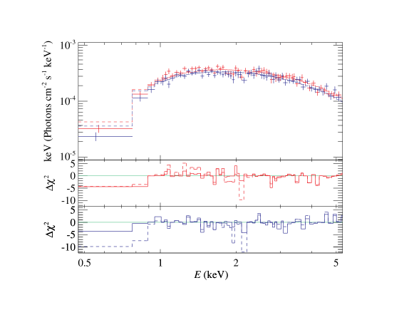
Figure 3: The effect of absorption on the spectral fits. Here, we zoom in on the low-energy region of the “high” Chandra data, at which absorption effects are evident, and we present model fits without any absorption included (dashed lines). The bottom panels show the resultant $\chi^{2}$ residuals with the sign of data-minus-model and the evident fit improvement –particularly around 2 keV– when absorption is incorporated into the model (solid lines) for each of the “high” spectra in turn. The inclusion of absorption increases the intrinsic flux of the underlying disk component in the fit, which has the effect of lowering $R_{\rm in}$, and accordingly increasing the inferred spin.

Our full, composite model is fitted to the six spectra (each of Chandra and NuSTAR for the three phase intervals) at once, and is structured as: crabcor $\times$ pileup(gabs $\times$ tbabs1 $\times$ [ warmabsorber1 $\times$ tbabs2 (simpl $\otimes$ kerrbb2) + warmabsorber2 $\times$ const (simpl $\otimes$ kerrbb2)]). Here, the constant term determines the contribution of X-ray emission scattered into our line of sight by the halo of electrons in the extended stellar wind. tbabs1 represents neutral absorption along the line of sight whereas tbabs2 gives absorption in the thick shell of wind during eclipse; accordingly, it is a fit term in the eclipsing “low” phase but the column is otherwise fixed to zero. warmabsorber1 describes the phase-dependent absorption by the wind of the source, while the column for warmabsorber2 is linked among all phases and describes the attenuation by absorption in the wind for the diffuse, scattered light. All parameters in simpl $\otimes$ kerrbb2 are linked between their two instances. (All warm absorber terms are linked to a single ionization parameter and turbulent velocity width, which turn out to be poorly constrained.) The illustration in Figure 2 shows the correspondence of these components to the structure of the system. The warm-absorber’s influence on the fit is presented in Figure 3 for the two “high” Chandra spectra.

Based on the similarity between IC 10 X–1 and the eclipsing high-mass black-hole binary M33 X–7, we adopt round fiducial values for the black-hole mass and inclination of $15\leavevmode\nobreak\ {\rm M}_{\odot}$ and $75\arcdeg$, respectively. Later, we will examine the mass-and-inclination dependence of our results. The fits, meanwhile, are only weakly sensitive to the value of the disk-viscosity term ($\alpha$), and here we pick a reference value of $\alpha=0.05$. We allow for differences with phase, including in ${\dot{M}}$ between intervals “high-1” and “high-2” (in the “low” interval, we match ${\dot{M}}$ to that obtained from “high-1”). Aside from the warm absorber column and ${\dot{M}}$ terms, all other parameters are tied among the observations.

We optimize the fit initially by directly fitting in xspec, and then for a more robust analysis a full exploration of the model is performed via Markov-Chain Monte Carlo (MCMC) using the emcee algorithm (Foreman-Mackey et al., 2013) following the setup described in Steiner et al. (2012b). Here, we apply usual noninformative priors to nearly all terms, either uniform in linear space for shape parameters (such as $a_{*}$ and $\Gamma$), or uniform on the logarithm for terms with no preferred scale (such as $N_{\rm H}$ or the normalizations). The single informative prior is on the crabcorr normalization for NuSTAR, which sets its cross-normalization relative to Chandra. We use a Gaussian centered on unity, with a width $\sigma=0.1$, based upon Madsen et al. (2015). From experience gained in Garciía et al. (2015), we favor employing a smaller number of walkers (we use 100, for 18 free parameters), in favor of running longer chains. Here, we run each walker for 50,000 steps, and discard the first 10,000 steps of each as burn-in. The auto-covariance of the parameters is significant, generally several hundred steps. Our report is comprised of the final 4 million aggregate steps, which amounts to many thousands of independent samplings for each parameter (the hundred-fold reduction is a result of the long-lived autocovariance in the chains). The best fitting black-hole model, which achieves $C^{2}/\nu=1.00$, is summarized in Table 2 and shown in Figure 4. The errors reported are (minimum-width) 90% confidence intervals. Notably, as was observed for M33 X–7, the system appears remarkably thermal, with scant allowance for nonthermal contribution from a corona. The spin obtained for this reference model is rather high and reasonably-well constrained, $a_{*}=0.85^{+0.04}_{-0.07}$ (90% confidence), where the error reflects statistical uncertainty only.

To elucidate the dependence of the spin constraint on the system’s mass and inclination, we have repeated our fit over a grid in mass and inclination, shown in Figure 5 (we have separately explored varying distance and $\alpha$; Section 5). A firm lower bound on the system inclination $i>63\arcdeg$ is possible due to the strong eclipse (Laycock et al., 2015a). Likewise, the fact that the system is X-ray persistent means that disk self-shadowing cannot be substantial, which precludes extremely high inclinations comparable to the disk scale height $h/r\sim 0.1$ (i.e., $i\lesssim 83\arcdeg$). We note that while the spin is strongly degenerate with changes in $M$ and $i$, there is nevertheless some sensitivity to the shape of the continuum for a given inclination and spin. There is a modest preference among the data for a “typical” BH mass $M\sim 5-20\leavevmode\nobreak\ {\rm M}_{\odot}$ (e.g., Özel et al. 2010), and for the inclination to be lower $i\lesssim 70\arcdeg$. This can be read from the white contours which are overlaid showing iso-surfaces of $\Delta C^{2}$ (measured relative to its global minimum). We note that the masses of the handful of wind-fed BHs are high ($\sim 10{\rm M}_{\odot}-15{\rm M}_{\odot}$) compared to transient BH systems (Özel et al. 2010). Across that mass range, the spin determination for IC 10 X–1 is generally high, with $a_{*}\gtrsim 0.8$ for most of the interval. This spin constraint for the wind-fed BHs mass range is illustrated in Figure 6. We have assumed a prior probability on each setting of $1/M$ (which has the effect of shifting spin toward lower values), as a naive proxy for a BH mass distribution which would favor lower masses, and apply a weight to each fit result according to its goodness ($w_{i}=\exp(-C^{2}/2)$). The dashed line in this figure illustrates a rough estimate of the effects of considering both a broad mass range and systematic uncertainty on the spin constraint. We note that if, despite its dubious standing, the large mass obtained by Silverman & Filippenko (2008) of $M>30\leavevmode\nobreak\ {\rm M}_{\odot}$ is later borne-out, then the corresponding spin must be extreme.

Table 2: IC 10 X–1 Black Hole Spectral Fits

Parameter	“Global” Setting	High-1	High-2	Low
$N_{\rm H}<{\rm tbabs1}>[10^{22}{\rm cm}^{-2}]$	$0.45\pm 0.06$	$\cdots$	$\cdots$	$\cdots$
warm-abs column $<$warmabs1$>$ [$10^{22}{\rm cm}^{-2}]$	$<1.6$	$<1.3$	$1.3-25.$	$\cdots$
warm-abs column $<$warmabs2$>$ [$10^{22}{\rm cm}^{-2}]$	$\cdots$	$\cdots$	$\cdots$	$<80$
$\Gamma$	$2.5^{+0.5}_{-0.7}$	$\cdots$	$\cdots$	$\cdots$
$f_{\rm sc}$	$<10\%$	$\cdots$	$\cdots$	$\cdots$
$a_{*}$	$0.85^{+0.04}_{-0.07}$	$\cdots$	$\cdots$	$\cdots$
$\dot{M}[10^{18}$ (g/s)]	$\cdots$	$2.4^{+0.7}_{-0.4}$	$2.3^{+0.7}_{-0.4}$	$\cdots$
$N_{\rm H}({\rm shell})<{\rm tbabs2}>[10^{22}{\rm cm}^{-2}]$	$\cdots$	$\cdots$	$\cdots$	$130^{+55}_{-40}$
$\tau_{\rm sc.em.}$	$0.124\pm 0.013$	$\cdots$	$\cdots$	$\cdots$
warm-abs log $\xi$	$1.3^{+2.0}_{-0.3}$	$\cdots$	$\cdots$	$\cdots$
warm-abs log ($v_{\rm turb}$/c)	$<0.5$  $\cdots$	$\cdots$	$\cdots$
NormToor&Seward,NuSTAR	$0.81\pm 0.05$	$\cdots$	$\cdots$	$\cdots$
$M[{\rm M}_{\odot}]$	15*	$\cdots$	$\cdots$	$\cdots$
$i$ [degrees]	75*	$\cdots$	$\cdots$	$\cdots$
$D$ [kpc]	750*	$\cdots$	$\cdots$	$\cdots$
$\alpha$	0.05*	$\cdots$	$\cdots$	$\cdots$
$\Delta\Gamma_{\rm Chandra}$	0.02*	$\cdots$	$\cdots$	$\cdots$
NormToor&Seward,Chandra	1.11*	$\cdots$	$\cdots$	$\cdots$
$\Delta\Gamma_{\rm NuSTAR}$	0.0*	$\cdots$	$\cdots$	$\cdots$
$E_{\rm gabs}$ [keV]	$2.02\pm 0.09$	$\cdots$	$\cdots$	$\cdots$
$\sigma_{\rm gabs}$ [keV]	$0.20^{+0.13}_{-0.09}$	$\cdots$	$\cdots$	$\cdots$
$N_{\rm gabs}$	$0.12^{+0.08}_{-0.05}$	$\cdots$	$\cdots$	$\cdots$
pileup g0	1.0*	$\cdots$	$\cdots$	$\cdots$
pileup alpha	0.7*	$\cdots$	$\cdots$	$\cdots$
pileup psffrac	0.95*	$\cdots$	$\cdots$	$\cdots$
$C^{2}/\nu$	773.43/774	$\cdots$	$\cdots$	$\cdots$

Note. — All ranges are 90% confidence intervals. Starred values were frozen in the fit.

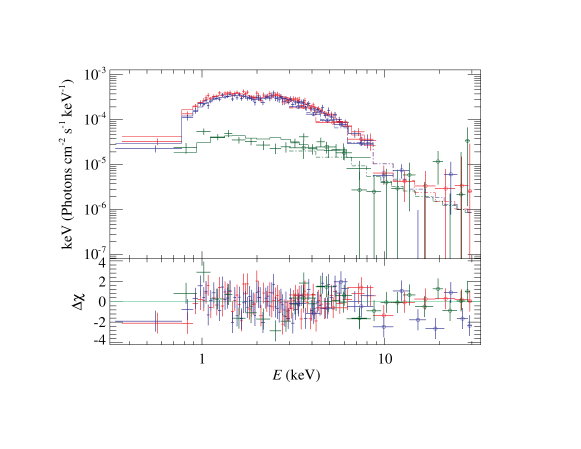
Figure 4: The best-fitting model and accompanying residuals to our joint Chandra and NuSTAR data set. The data have been rebinned for plotting purposes only. The three time intervals marked in Fig. 1 are fitted jointly. Fit parameters are given in Table 2. “High-1” and “high-2” are shown in red and blue, respectively, and green shows the “low” data for both Chandra and NuSTAR. NuSTAR data are marked with open circles, and the NuSTAR spectral models are given with dot-dashed lines, whereas Chandra’s model fits are solid lines.

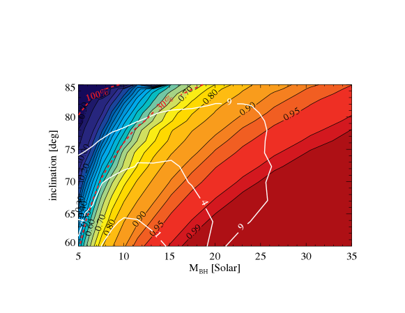
Figure 5: Spin as a function of the BH’s mass and inclination. $\Delta C^{2}$ contours are overlaid in white, marking out the weakly preferred values of mass, spin, and inclination. The statistical uncertainty in spin, while not shown here, scales nonlinearly in spin, but is rather constant in units of $\Delta R/R_{\rm ISCO}$ (the $1\sigma$ error being $\approx 5.5\%$). The red dashed lines show contours of constant luminosity, in percentage of the Eddington limit. The lower dashed line at 30% Eddington separates the region at which the model is within the thin-disk limit (below and to the right of the line) from the region for which the disk would be appreciably thick.

5 Discussion

Our thin-disk model kerrbb2 delivers reliable estimates of spin only at luminosities $L\lesssim 30\%L_{\rm Eddington}$ and for spectra that are disk-dominated (McClintock et al., 2014). The spectrum of IC 10 X–1 amply meets these two criteria for values of $M$ characteristic of the wind-fed BHs ($\sim 10-15{\rm M}_{\odot}$) and for the favored range of $i$ ($\sim 65-75\arcdeg$). However, at sufficiently low mass and high inclination the luminosity exceeds 30% of Eddington, as indicated in Figure 5 by the red-dashed contour labeled “30%”. In this regime, our model underpredicts the spin and our results become increasingly unreliable with increasing luminosity (see, e.g., Straub et al. 2011). (We note that here we use the usual definition of the Eddington luminosity, namely $L_{\rm Edd}=1.3\times 10^{38}{\rm erg\leavevmode\nobreak\ s^{-1}}(M/{\rm M}_{\odot})$, which describes the luminosity at which radiation in an isotropic hydrogen sphere is at equilibrium with gravity. However, the corresponding luminosity at which this equilibrium is reached for a He atmosphere can be a factor of 2 higher.)

Our spin estimates rely on a standard version of bhspec which assumes solar metallicity. While this is not ideal, it is likely a reasonable value given that the depressed metallicity of IC 10 ($\sim 10-20$% that of the Galaxy) is compensated by the hydrogen-depleted atmosphere of the W-R companion (Clark & Crowther, 2004). We assessed this source of uncertainty using alternate bhspec models with metallicites that are 0.1 and 0.5 the solar value and found that the effect on our results is negligible. We similarly explored the effect of varying $\alpha$; switching between the two default values of 0.01 and 0.1 has a $\sim 3-5\%$ effect on $R_{\rm ISCO}$. The uncertainty in the distance has the biggest effect, resulting in an error in $R_{\rm ISCO}$ of $\sim 6\%$, which is comparable to the precision of the spectral fit. In sum total, the systematic uncertainty in the spin constraint is $\sim 10\%$ on $R_{\rm ISCO}$; for reference, this is equivalent to $\sigma_{a_{*}}=0.045$ at $a_{*}=0.85$.

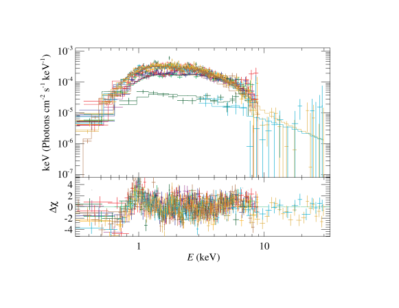
Figure 7: As in Fig. 4, but including a dozen other Chandra and XMM-Newton spectra. These spectra span a factor $\sim 2$ in luminosity. Although the other data lack high energy coverage, we find they are quite consistent with our broadband fit for spin.

In addition to our November 2014 observation, Chandra made three $30-50$ ks observations of IC 10 X–1 as well as several 15 ks snapshot observations. The frame times were longer for these observations than for ours and 10–20% of the events are piled up. XMM-Newton observed IC 10 X–1 on two occasions with exposure times of 45 and 135 ks. We analyzed all of these out-of-eclipse data. Figure 7 shows fits to the Chandra and XMM-Newton spectra, along with our data. Only the Chandra data were corrected for pileup. All the system parameters were tied except for $\dot{M}$, $f_{\rm sc}$, and the column of warmabsorber1, which were allowed to vary from observation to observation. Apart from the November 2014 data, the constraints on $f_{\rm sc}$ are weak because of the lack of high-energy coverage.

Note that the source luminosity from all epochs spans a factor $\sim 2$ (Figure 7), in line with the range observed in other wind-fed X-ray binary systems (e.g., Cyg X–1). Unfortunately, none of the spectra, apart from the November 2014 observation, can deliver an independent and reliable estimate of spin primarily because of the limited bandwidth, which does not allow one to isolate the thermal component from the Compton component. For example, consider the 135 ks XMM-Newton spectrum which has the highest $S/N$. Fits to this spectrum allow a broad range for the normalization of the Compton component, $f_{\rm sc}=0.02-0.32$ ($1\sigma$ level of confidence).

We can nevertheless determine for the complete collection of spectra that the spin is very similar to the value we obtained in Section 4.2 by analyzing just the Chandra plus NuSTAR spectra. A joint fit to all the spectra in Figure 7 yields $a_{*}=0.76\pm 0.03$ where we have assumed that scattered light is a constant fraction (set by the “low” spectrum) of the disk emission. We obtain a poorer fit in this case, with $C^{2}/\nu=1.44$. While it is possible that variation in the wind scattering or inadequate modeling of pileup may be responsible for the poorer fit and marginal decrease in spin, we note that the luminosities of several of the spectra exceed our nominal limit of 30% of Eddington, which can depress the spin value.

IC 10 X–1 has characteristics very similar to the other eclipsing BH system in the Local Group, M33 X–7, which is comprised of a $70{\rm M}_{\odot}$ O-giant and a $\sim 15{\rm M}_{\odot}$ BH (Orosz et al., 2007). For this 3.5-day period system, the duration of the X-ray eclipse, including the effects of the O-star’s extended wind ($\dot{M}_{\rm wind}\approx 2.6{\times}10^{-6}M_{\odot}$ yr^-1), is 0.15 in phase, with the full width and speed of ingress strongly influenced by the absorption and scattering of X-rays in the wind.

As was explored for M33 X–7 (Orosz et al., 2007), and as considered for IC 10 X–1 by Laycock et al. (2015b), we compute the Bondi-Holye-Littleton (BHL) rate of mass capture by IC 10 X–1 in order to check its compatibility with the mass supply and efficiency of the BH (${\dot{M}}\approx 10^{18}-10^{19}$ g s^-1 from our fits over the allowed range of $M$ and $i$ in Figure 5). From Edgar (2004), for a supersonic wind,

$$\dot{M}_{\rm BHL}=\frac{4\pi G^{2}M^{2}\rho}{v^{3}},$$ (1)

where $v$ is the relative speed of the wind and $\rho$ is the wind’s density. From Clark & Crowther (2004), we adopt $v_{\infty}=1750$ km s^-1, and use the approximate scaling law:

$$v(r)=v_{\infty}\left(1-\frac{R}{r}\right)^{\beta},$$ (2)

(Crowther, 2007), where $R$ is the stellar radius and $\beta\approx 1$. At the binary separation $a\sim 20R_{\sun}$ (Laycock et al., 2015b) we estimate roughly $v\approx 1600$ km s^-1, which includes the moderate effect of orbital motion (appropriate for the range of typical BH masses). Using the mass-loss rate from Clark & Crowther (2004) of $\dot{M}_{\rm wind}=10^{-5}\leavevmode\nobreak\ {\rm M}_{\odot}\leavevmode\nobreak\ {\rm yr}^{-1}$, the predicted electron and mass densities in the helium-dominated wind are $n_{e}\approx 4\times 10^{10}{\rm cm}^{-3}$, and $\rho\approx 2\times 10^{-13}$ g cm^-3. For the range of BH masses in question $\sim 5-40{\rm M}_{\odot}$, ${\dot{M}}_{\rm BHL}$ comes out in the range $2\times 10^{17}-2\times 10^{19}$ g s^-1, with larger values corresponding to solutions for higher BH masses. Although the estimate is crude, it demonstrates that mass capture and subsequent accretion from the W-R wind is fully capable of powering the BH.

We can check on the above prediction for the wind profile by noting that the change in the line-of-sight column of the warm absorber, while weakly constrained, grows over the orbit by, very roughly $\sim 10^{22}$ cm^-2 (noting that as determined from the MCMC analysis, the increase is at a mere 2$\sigma$ significance), being largest when eclipsed. Because the source has reached a pathlength greater by $\sim a$, the density in the wind is $n_{e}\approx\Delta N/a\approx 10^{10}\leavevmode\nobreak\ {\rm cm}^{-3}$. When accounting for the abundance differences between IC 10 and the Galaxy, the absence of H in the W-R star, again the dearth of metals wash out to a correction factor of roughly unity. This bolsters the above picture for mass-loss in the system and underscores the assumed association between warm absorber and the W-R wind. Finally, we observe that a simple estimate for the ionization pattern far from the BH at high latitudes is that the ionization parameter $\xi\sim L/nr^{2}$ should be of order thousands, and that given sufficient resolution one would expect to find a dark cone with a factor $\sim 2$ lower ionization in the shadow of the star. In practice, the constraints on the ionization parameter from the observations are weak, and so we can only say that our results are not in conflict with this value.

6 Conclusions

In summary, using a Chandra/NuSTAR observation we have demonstrated that the compact primary in IC 10 X–1 is implausible as a neutron star and therefore a black hole explanation is highly likely. Although the mass is uncertain, for any pairing of black hole mass $M$ and inclination $i$ we have determined a unique and precise estimate of the spin parameter $a_{*}$ using the continuum-fitting method. The strongly disk-dominated spectrum of IC 10 X–1 makes this method an especially reliable one. Meantime, this distant source ($\sim 750$ kpc) is presently too faint for application of the Fe-line method. NuSTAR’s high-energy coverage picks up precisely where Chandra’s effective area is falling. Critically, the mutual capabilities of Chandra and NuSTAR allow one to firmly anchor the power-law component and thereby isolate and reliably model the thermal component.

Our excellent data set allows us to obtain a net precision of $\sigma_{a_{*}}\approx 0.05$. However, we are hampered by a serious limitation, namely the uncertain mass of the black hole. We meet this challenge by computing the spin as a function of $M$ and $i$ over a broad range of these parameters; our constraints on $a_{*}$ are displayed in Figure 5. We find that if the mass is comparable to that in the other wind-fed systems (a value significantly above the typical mass of a transient black hole) then the spin of IC 10 X–1 is likely be high ($a_{*}\gtrsim 0.7$), as it is for the other wind-fed systems.

The massive W-R companion implies a young age for IC 10 X–1, which in turn implies that the high spin was imparted to the black hole during its birth event. It is important now to attempt to estimate the mass of the black hole because the combination of high-mass and high-spin would strengthen the apparent dichotomy between wind-fed and transient black hole X-ray binaries (Section 1), which would point to a distinct formation channel for BH systems with massive companions (e.g., Kochanek 2015). Presently, while we can rule against a neutron-star primary, the jury is still out on the mass – and hence the spin – of the BH in IC 10 X–1. If in future work the mass of the BH can be constrained, then our results provide an immediate complementary estimate of its spin.

Figure 6: A probability distribution estimate for spin, in which fit results have been weighted according to the goodness of fit. The solid line shows the spin distribution associated with BH masses in the wind-fed range, $10-15\leavevmode\nobreak\ {\rm M}_{\odot}$, and allowing for the full range of allowed inclinations. However, secondary model parameters (e.g., $\alpha$ and $D$) have been merely fixed at their nominal values. The dashed line shows a complementary constraint, in which we crudely assess a broad range of uncertainty by allowing for many unknowns, e.g., we consider the full range of explored BH masses, from $5-35\leavevmode\nobreak\ {\rm M}_{\odot}$, again consider all allowed inclinations, and similarly incorporate the uncertainty in $D$ and the full span of possible settings for $\alpha$.

References

- Arnaud (1996) Arnaud, K. A. 1996, in Astronomical Society of the Pacific Conference Series, Vol. 101, Astronomical Data Analysis Software and Systems V, ed. G. H. Jacoby & J. Barnes, 17
- Barnard et al. (2014) Barnard, R., Steiner, J. F., Prestwich, A. F., Stevens, I. R., Clark, J. S., & Kolb, U. C. 2014, ApJ, 792, 131
- Barret & Olive (2002) Barret, D., & Olive, J.-F. 2002, ApJ, 576, 391
- Bauer & Brandt (2004) Bauer, F. E., & Brandt, W. N. 2004, ApJ, 601, L67
- Binder et al. (2015) Binder, B., Gross, J., Williams, B. F., & Simons, D. 2015, MNRAS, 451, 4471
- Bogomazov (2014) Bogomazov, A. I. 2014, Astronomy Reports, 58, 126
- Brandt et al. (1997) Brandt, W. N., Ward, M. J., Fabian, A. C., & Hodge, P. W. 1997, MNRAS, 291, 709
- Brenneman (2013) Brenneman, L. 2013, Measuring the Angular Momentum of Supermassive Black Holes
- Cash (1979) Cash, W. 1979, ApJ, 228, 939
- Church et al. (2012) Church, M. J., Gibiec, A., Bałucińska-Church, M., & Jackson, N. K. 2012, A&A, 546, A35
- Clark & Crowther (2004) Clark, J. S., & Crowther, P. A. 2004, A&A, 414, L45
- Crowther (2007) Crowther, P. A. 2007, ARA&A, 45, 177
- Davis (2001) Davis, J. E. 2001, ApJ, 562, 575
- Davis & Hubeny (2006) Davis, S. W., & Hubeny, I. 2006, ApJS, 164, 530
- Demers et al. (2004) Demers, S., Battinelli, P., & Letarte, B. 2004, A&A, 424, 125
- Dickey & Lockman (1990) Dickey, J. M., & Lockman, F. J. 1990, ARA&A, 28, 215
- Edgar (2004) Edgar, R. 2004, New A Rev., 48, 843
- Fabrika (2004) Fabrika, S. 2004, Astrophysics and Space Physics Reviews, 12, 1
- Foreman-Mackey et al. (2013) Foreman-Mackey, D., Hogg, D. W., Lang, D., & Goodman, J. 2013, PASP, 125, 306
- Fragos & McClintock (2015) Fragos, T., & McClintock, J. E. 2015, ApJ, 800, 17
- Gallo et al. (2005) Gallo, E., Fender, R., Kaiser, C., Russell, D., Morganti, R., Oosterloo, T., & Heinz, S. 2005, Nature, 436, 819
- Gandolfi et al. (2012) Gandolfi, S., Carlson, J., & Reddy, S. 2012, Phys. Rev. C, 85, 032801
- Garciía et al. (2015) Garciía, J. A., Steiner, J. F., McClintock, J. E., Remillard, R. A., Grinberg, V., & Dauser, T. 2015, ApJ, 813, 84
- Gierliński & Done (2004) Gierliński, M., & Done, C. 2004, MNRAS, 349, L7
- Heinz (2002) Heinz, S. 2002, A&A, 388, L40
- Ho & Heinke (2009) Ho, W. C. G., & Heinke, C. O. 2009, Nature, 462, 71
- Homan et al. (2010) Homan, J., et al. 2010, ApJ, 719, 201
- Homan et al. (2007) —. 2007, ApJ, 656, 420
- Inogamov & Sunyaev (1999) Inogamov, N. A., & Sunyaev, R. A. 1999, Astronomy Letters, 25, 269
- Ishida et al. (2011) Ishida, M., et al. 2011, PASJ, 63, 657
- Kallman & Bautista (2001) Kallman, T., & Bautista, M. 2001, ApJS, 133, 221
- Kim et al. (2009) Kim, M., Kim, E., Hwang, N., Lee, M. G., Im, M., Karoji, H., Noumaru, J., & Tanaka, I. 2009, ApJ, 703, 816
- Kniazev et al. (2008) Kniazev, A. Y., Pustilnik, S. A., & Zucker, D. B. 2008, MNRAS, 384, 1045
- Kochanek (2015) Kochanek, C. S. 2015, MNRAS, 446, 1213
- Kulkarni et al. (2011) Kulkarni, A. K., et al. 2011, MNRAS, 414, 1183
- Laycock et al. (2015a) Laycock, S. G. T., Cappallo, R. C., & Moro, M. J. 2015a, MNRAS, 446, 1399
- Laycock et al. (2015b) Laycock, S. G. T., Maccarone, T. J., & Christodoulou, D. M. 2015b, ArXiv e-prints
- Li et al. (2005) Li, L.-X., Zimmerman, E. R., Narayan, R., & McClintock, J. E. 2005, ApJS, 157, 335
- Lin et al. (2009a) Lin, D., Altamirano, D., Homan, J., Remillard, R. A., Wijnands, R., & Belloni, T. 2009a, ApJ, 699, 60
- Lin et al. (2007) Lin, D., Remillard, R. A., & Homan, J. 2007, ApJ, 667, 1073
- Lin et al. (2009b) —. 2009b, ApJ, 696, 1257
- Lin et al. (2010) —. 2010, ApJ, 719, 1350
- Lin et al. (2012) Lin, D., Remillard, R. A., Homan, J., & Barret, D. 2012, ApJ, 756, 34
- Madsen et al. (2015) Madsen, K. K., et al. 2015, ArXiv e-prints
- McClintock et al. (2014) McClintock, J. E., Narayan, R., & Steiner, J. F. 2014, Space Sci. Rev., 183, 295
- McClintock et al. (2006) McClintock, J. E., Shafee, R., Narayan, R., Remillard, R. A., Davis, S. W., & Li, L.-X. 2006, ApJ, 652, 518
- Noble et al. (2009) Noble, S. C., Krolik, J. H., & Hawley, J. F. 2009, ApJ, 692, 411
- Noble et al. (2010) —. 2010, ApJ, 711, 959
- Novikov & Thorne (1973) Novikov, I. D., & Thorne, K. S. 1973, in Black Holes (Les Astres Occlus), 343–450
- Orosz et al. (2007) Orosz, J. A., et al. 2007, Nature, 449, 872
- Özel (2013) Özel, F. 2013, Reports on Progress in Physics, 76, 016901
- Özel et al. (2010) Özel, F., Psaltis, D., Narayan, R., & McClintock, J. E. 2010, ApJ, 725, 1918
- Pakull & Angebault (1986) Pakull, M. W., & Angebault, L. P. 1986, Nature, 322, 511
- Pasham et al. (2013) Pasham, D. R., Strohmayer, T. E., & Mushotzky, R. F. 2013, ApJ, 771, L44
- Popham & Sunyaev (2001) Popham, R., & Sunyaev, R. 2001, ApJ, 547, 355
- Prestwich et al. (2007) Prestwich, A. H., et al. 2007, ApJ, 669, L21
- Revnivtsev & Gilfanov (2006) Revnivtsev, M. G., & Gilfanov, M. R. 2006, A&A, 453, 253
- Reynolds (2014) Reynolds, C. S. 2014, Space Sci. Rev., 183, 277
- Risaliti et al. (2013) Risaliti, G., et al. 2013, Nature, 494, 449
- Sakai et al. (1999) Sakai, S., Madore, B. F., & Freedman, W. L. 1999, ApJ, 511, 671
- Sánchez-Sutil et al. (2008) Sánchez-Sutil, J. R., Martí, J., Combi, J. A., Luque-Escamilla, P., Muñoz-Arjonilla, A. J., Paredes, J. M., & Pooley, G. 2008, A&A, 479, 523
- Sanna et al. (2008) Sanna, N., et al. 2008, ApJ, 688, L69
- Silverman & Filippenko (2008) Silverman, J. M., & Filippenko, A. V. 2008, ApJ, 678, L17
- Steiner & McClintock (2012) Steiner, J. F., & McClintock, J. E. 2012, ApJ, 745, 136
- Steiner et al. (2014) Steiner, J. F., McClintock, J. E., Orosz, J. A., Remillard, R. A., Bailyn, C. D., Kolehmainen, M., & Straub, O. 2014, ApJ, 793, L29
- Steiner et al. (2012a) Steiner, J. F., McClintock, J. E., & Reid, M. J. 2012a, ApJ, 745, L7
- Steiner et al. (2010) Steiner, J. F., McClintock, J. E., Remillard, R. A., Gou, L., Yamada, S., & Narayan, R. 2010, ApJ, 718, L117
- Steiner et al. (2009) Steiner, J. F., Narayan, R., McClintock, J. E., & Ebisawa, K. 2009, PASP, 121, 1279
- Steiner et al. (2012b) Steiner, J. F., et al. 2012b, MNRAS, 427, 2552
- Straub et al. (2011) Straub, O., et al. 2011, A&A, 533, A67
- Suleimanov et al. (2011) Suleimanov, V., Poutanen, J., & Werner, K. 2011, A&A, 527, A139
- Toor & Seward (1974) Toor, A., & Seward, F. D. 1974, AJ, 79, 995
- Vacca et al. (2007) Vacca, W. D., Sheehy, C. D., & Graham, J. R. 2007, ApJ, 662, 272
- Verner et al. (1996) Verner, D. A., Ferland, G. J., Korista, K. T., & Yakovlev, D. G. 1996, ApJ, 465, 487
- Vilhu et al. (2009) Vilhu, O., Hakala, P., Hannikainen, D. C., McCollough, M., & Koljonen, K. 2009, A&A, 501, 679
- Walton et al. (2012) Walton, D. J., Reis, R. C., Cackett, E. M., Fabian, A. C., & Miller, J. M. 2012, MNRAS, 422, 2510
- Wang et al. (2005) Wang, Q. D., Whitaker, K. E., & Williams, R. 2005, MNRAS, 362, 1065
- Wang et al. (2003) Wang, X. Y., Dai, Z. G., & Lu, T. 2003, ApJ, 592, 347
- Wilms et al. (2000) Wilms, J., Allen, A., & McCray, R. 2000, ApJ, 542, 914
- Yang & Skillman (1993) Yang, H., & Skillman, E. D. 1993, AJ, 106, 1448
- Zhu et al. (2012) Zhu, Y., Davis, S. W., Narayan, R., Kulkarni, A. K., Penna, R. F., & McClintock, J. E. 2012, MNRAS, 424, 2504
- Zimmerman et al. (2005) Zimmerman, E. R., Narayan, R., McClintock, J. E., & Miller, J. M. 2005, ApJ, 618, 832