Implications on the cosmic coincidence by a dynamical extrinsic curvature

Abstract

In this work, we apply the smooth deformation concept in order to obtain a modification of Friedmann equations. It is shown that the cosmic coincidence can be at least alleviated using the dynamical properties of the extrinsic curvature. We investigate the transition from nucleosynthesis to the coincidence era obtaining a very small variation of the ratio $r=\frac{\rho_{m}}{\rho_{ext}}$, that compares the matter energy density to extrinsic energy density, compatible with the known behavior of the deceleration parameter. We also show that the calculated “equivalence” redshift matches the transition redshift from a deceleration to accelerated phase and the coincidence ceases to be. The dynamics on $r$ is also studied based on Hubble parameter observations as the latest Baryons Acoustic Oscillations/Cosmic Microwave Background Radiation (BAO/CMBR) + SNIa.

I Introduction

Modifications of gravity at very large scales have been predominantly associated with the existence of extra dimensions, an idea that has been explored in various theories beyond the standard model of particle physics. As proposed in ADD , these extra dimensions may also provide a possible explanation for the huge difference between the two fundamental energy scales in nature, namely, the electroweak and Planck scales [$M_{Pl}/m_{EW}\sim 10^{16}$]. Essentially, if our four-dimensional space-time is embedded in a higher dimensional space, then the gravitational field can also propagate along the extra dimensions, while the standard gauge interactions remain confined to the four-dimensional spacetime. The impact of such program in theoretical and observational cosmology has been substantial and discussed at length as, e.g., in Refs. RS ; RS1 ; 7 ; Tsujikawa ; 9 ; maartens ; maeda ; sepangi ; sepangi1 ; QBW ; rostami ; jalal ; heydari with or without junction conditions. However, the majority of contributions on this theme are string (or brane) inspired models, in which the brane-world is generated by the motion of a three-dimensional brane in the bulk.

In a different approach, we have explored the physical applications and implications of using the concept of smooth deformations of Nash’s theorem Nash where the bulk geometry is defined by the Einstein-Hilbert principle of smooth curvature and only gravity necessarily propagates in the extra dimensions. In that respect, it should be emphasized that the four-dimensionality of the embedded space-time is regarded as a consequence of the structure of the gauge field equations, which is applicable to all embedded space-times (and not just to a fixed boundary). Such extended notion of confinement is consistent with the Einstein-Hilbert dynamics for the bulk geometry, and also to the extrinsic curvature satisfying the Gupta equations Gupta ; GDEI for spin-2 fields in space-time.

In what follows, we focus on the coincidence problem, sometimes referred as the “new” cosmological constant (CC) problem weinberg ; weinberg2 ; shapiro1 ; shapiro2 ; shapiro3 which, in short, refers to the lack of a proper explanation of the present-day contributions of vacuum energy density $\Omega^{0}_{\Lambda}$ and the matter energy density $\Omega^{0}_{m}$ that are roughly the same order, i.e, $\Omega^{0}_{m}\sim\Omega^{0}_{\Lambda}$ since CC is considered the main cause of the accelerated expansion of the universe. Hence, as commonly stated, it seems we are living is a very special phase to observe it.

In this work, we study a process to at least alleviate the cosmic coincidence through the introduction of the dynamics of the extrinsic curvature $k_{\mu\nu}$, interpreted as an additional component to the gravitational field. Then, CC is totally uncorrelated to this process and is not considered here. We also analyze the necessary conditions of our model in order to do not jeopardize the nucleosynthesis from the standard cosmological model and the compatibility with the declaration parameter in different eras. Moreover, using a modified Friedmann equations we look for an expression in order to relate the ratio $r=\frac{\rho_{m}}{\rho_{ext}}$ to the Hubble parameter $H$, where $\rho_{m}$ denotes the total matter energy density (including cold dark matter contribution) and the $\rho_{ext}$ density denotes the extrinsic energy density, in order to get information of the dynamics on the ratio $r$. Finally, remarks are presented in the conclusion section.

II Modified Friedmann equations

The traditional gravitational perturbation mechanisms in cosmology are essentially plagued by coordinate gauges, mostly inherited from the group of diffeomorphisms of general relativity. Fortunately there are some very successful criteria to filter out the latter perturbations Bardeen ; Geroch ; Walker , but they still depend on a choice of a perturbative model. A lesser known, but far more general approach to gravitational perturbation can be derived from a theorem due to John Nash, showing that any Riemannian geometry can be generated by a continuous sequence of local infinitesimal increments of a given geometry Nash ; Greene .

Nash’s theorem solves an old dilemma of Riemannian geometry, namely that the Riemann tensor is not sufficient to make a precise statement about the local shape of a geometrical object or a manifold. The simplest example is given by a 2-dimensional Riemannian manifold, where the Riemann tensor has only one component $R_{1212}$ which coincides with the Gaussian curvature. Thus, a flat Riemannian 2-manifold defined by $R_{1212}=0$ may be interpreted as a plane, a cylinder or a even a helicoid, in the sense of Euclidean geometry. Riemann regarded his concept of curvature as defining an equivalent class of manifolds instead of a specific one Riemann . While such equivalence of forms is mathematically interesting, it is less than adequate to derive physical conclusions from today’s sophisticated astronomical observations.

Using only differentiable (non-analytic) properties, Nash showed that any other embedded Riemannian geometry can be generated by differentiable perturbations with a perturbed metric $\tilde{g}_{\mu\nu}=g_{\mu\nu}+\delta g_{\mu\nu}$, where

$$\delta g_{\mu\nu}=-2k_{\mu\nu a}\delta y^{a}\;,$$ (1)

where $\delta y^{a}$ is an infinitesimal displacement in one of the extra dimension and $k_{\mu\nu}$ is the non-perturbed extrinsic curvature GDEI ; QBW . From this new metric, we obtain a new extrinsic curvature $k_{\mu\nu}$ and the procedure can be repeated indefinitely:

$$\tilde{g}_{\mu\nu}=g_{\mu\nu}+\delta y^{a}\,k_{\mu\nu a}+\delta y^{a}\delta y^{b}\,g^{\rho\sigma}k_{\mu\rho a}k_{\nu\sigma b}+\cdots\;,$$ (2)

and gives the possibility to generate new geometries by smooth deformations.

In our description of the universe, we use the Friedmann-Lemaître-Robertson-Walker (FLRW) line element in coordinates $(r,\theta,\phi,t)$ which is given by

$$ds^{2}=\;-dt^{2}+a^{2}\left[dr^{2}+f_{\kappa}^{2}(r)\left(d\theta^{2}+\sin^{2}\theta d\varphi^{2}\right)\right]\;,$$ (3)

where the set of functions $f_{\kappa}(r)=\sin r$, $r$,$\sinh r$ corresponds to spatial curvatures $\kappa$ = (1, 0, -1), and the function $a=a(t)$ is the expansion parameter. This geometry can be regarded as a four-dimensional hypersurface dynamically evolving in a five-dimensional bulk space with constant curvature. Since Nash’s smooth deformations are applied to the embedding process and the FLRW geometry is completely embedded in five-dimensions rosen ; szek ; maia , the coordinate $y$, usually noticed in ridig embedded models, e.g RS ; RS1 , is omitted in Eq.(3). Concerning notation, we use the same conventions as posed in GDEI .

The bulk geometry is actually defined by the Einstein-Hilbert principle, which leads to the Einstein equations

$${\mathcal{R}}_{AB}-\frac{1}{2}{\mathcal{R}}{\mathcal{G}}_{AB}=\alpha_{*}T^{*}_{AB}\;,$$ (4)

where $T^{*}_{AB}$ denotes the energy-momentum tensor of the known sources. For the present application, capital Latin indices run from 1 to 5. Small case Latin indices refer to the only one extra dimension considered. All Greek indices refer to the embedded space-time counting from 1 to 4.

The confinement of gauge fields and ordinary matter are a standard assumption specially in what concerns the brane-world program as a part of the solution of the hierarchy problem of the fundamental interactions: the four-dimensionality of space-time is a consequence of the invariance of Maxwell’s equations under the Poincaré group. Such condition was latter seen to be proper to all gauge fields expressed in terms of differential forms and their duals. However, in spite of many attempts, gravitation, in the sense of Einstein, does not fit in such scheme. Thus, while all known gauge fields are confined to the four-dimensional submanifold, gravitation as defined in the whole bulk space by the Einstein-Hilbert principle, propagates in the bulk. The proposed solution of the hierarchy problem says that gravitational energy scale is somewhere within TeV scale.

The most general expression of this confinement is that the confined components of $T_{AB}$ are proportional to the energy-momentum tensor of general relativity: $\alpha_{*}T_{\mu\nu}=-8\pi GT_{\mu\nu}$. On the other hand, since only gravity propagates in the bulk we have $T_{\mu a}=0$ and $T_{ab}=0$.

Since we are dealing with embedded space-times, we need to write the induced field equations of the embedded geometry which in fact they result from the geometrical features of the bulk space by the integration of the Gauss-Codazzi equations (GDEI, ; QBW, ). To this end, we can define a five-dimensional local embedding with an embedding map $\mathcal{Z}\mathrel{\mathop{\mathchar 58\relax}}V_{4}\rightarrow V_{5}$. We admit that $\mathcal{Z}^{\mu}$ is a regular and differentiable map with $V_{4}$ and $V_{5}$ being the embedded space-time and the bulk, respectively. The components $\mathcal{Z}^{A}=\;f^{A}(x^{1},...,x^{4})$ associate with each point of $V_{4}$ a point in $V_{5}$ with coordinates $\mathcal{Z}^{A}$. These coordinates are the components of the tangent vectors of $V_{4}$. Moreover, taking the tangent, vector and scalar components of Eq.(4) defined in the Gaussian frame veilbein $\{\mathcal{Z}^{A}_{,\mu},\eta^{A}\}$, where $\eta^{A}$ are the components of the normal vectors of $V_{4}$, one can obtain the following equations in the embedded spacetime (GDEI, ; QBW, )

$$R_{\mu\nu}-\frac{1}{2}Rg_{\mu\nu}-Q_{\mu\nu}=-8\pi GT_{\mu\nu}\;,\hskip 11.38109pt$$ (5)

$$k_{\mu;\;\rho}^{\;\rho}-h_{,\mu}=0\;,$$ (6)

where $T_{\mu\nu}$ is the four-dimensional energy-momentum tensor of the perfect fluid expressed in co-moving coordinates as

$$T_{\mu\nu}=(p+\rho)U_{\mu}U_{\nu}+p\;g_{\mu\nu},\;\;\;U_{\mu}=\delta_{\mu}^{4}\;.$$

The quantity $Q_{\mu\nu}$ is a geometrical term defined as

$$Q_{\mu\nu}=g^{\rho\sigma}k_{\mu\rho}k_{\nu\sigma}-k_{\mu\nu}h-\frac{1}{2}\left(K^{2}-h^{2}\right)g_{\mu\nu}\;,$$ (7)

where $h=g^{\mu\nu}k_{\mu\nu}$, $h^{2}=h.h$ and $K^{2}=k^{\mu\nu}k_{\mu\nu}$. It follows that the quantity $Q_{\mu\nu}$ is conserved in the sense that

$$Q^{\mu\nu}{}_{;\nu}=0\;,$$ (8)

where the symbol $(;)$ denotes the four-dimensional induced covariant derivative.

The general solution for Eq.(6) using the FLRW metric is

$$k_{ij}=\frac{b}{a^{2}}g_{ij},\;\;k_{44}=\frac{-1}{\dot{a}}\frac{d}{dt}\frac{b}{a}$$

in this case $i,j=1,2,3$, where the bending function $b(t)=k_{11}$ is an arbitrary function of time, resulting from the Codazzi homogeneous equations in Eq.(6).

From the calculations of Eq.(5) and Eq.(6), one can obtain

$$k_{44}=-\frac{b}{a^{2}}\left(\frac{B}{H}-1\right)g_{44},\;h=\frac{b}{a^{2}}\left(\frac{B}{H}+2\right),$$ (9)

$$K^{2}=\frac{b^{2}}{a^{4}}\left(\frac{B^{2}}{H^{2}}-2\frac{B}{H}+4\right),$$ (10)

$$Q_{ij}=\frac{b^{2}}{a^{4}}\left(2\frac{B}{H}-1\right)g_{ij},\;Q_{44}=-\frac{3b^{2}}{a^{4}},$$ (11)

$$Q=-(K^{2}-h^{2})=\frac{6b^{2}}{a^{4}}\frac{B}{H}\;.$$ (12)

In the case of Eq.(11), consider $i,j=1,2,3$. The usual Hubble parameter in terms of the expansion scaling factor $a(t)=a$ is denoted by $H=\dot{a}/a$ and the extrinsic parameter $B=\dot{b}/b$, where the dot holds for the ordinary time derivative. It is important to point out that the determination of the bending function $b(t)$ comes from the determination of dynamical equations for extrinsic curvature. To this end, we used the “vacuum” Gupta equations

$$\mathcal{F}_{\mu\nu}=0\;,$$ (13)

where, unlike the case of Einstein’s equations, we do not have the equivalent to the Newtonian weak field limit and we cannot tell about the nature of the source term of Eq.(13) based on current experience and observations. Accordingly, the “f-Ricci tensor” and the “f-Ricci scalar”, defined with $f_{\mu\nu}$ are, respectively,

$${\cal F}_{\mu\nu}=f^{\alpha\lambda}\mathcal{F}_{\nu\alpha\lambda\mu}\;\;\mbox{and}\;\;\mathcal{F}=f^{\mu\nu}\mathcal{F}_{\mu\nu}$$

and also the “f-Riemann tensor”

$$\mathcal{F}_{\nu\alpha\lambda\mu}=\;\partial_{\alpha}\Upsilon_{\mu\lambda\nu}-\;\partial_{\lambda}\Upsilon_{\mu\alpha\nu}+\Upsilon_{\alpha\sigma\mu}\Upsilon_{\lambda\nu}^{\sigma}-\Upsilon_{\lambda\sigma\mu}\Upsilon_{\alpha\nu}^{\sigma}$$

constructed from a “connection” associated with $k_{\mu\nu}$. We stress that the geometry of the embedded space-time has been previously defined by $g_{\mu\nu}$. Hence, we define the tensors

$$f_{\mu\nu}=\frac{2}{K}k_{\mu\nu},\;\;\mbox{and}\;\;f^{\mu\nu}=\frac{2}{K}k^{\mu\nu}\;,$$ (14)

so that $f^{\mu\rho}f_{\rho\nu}=\delta^{\mu}_{\nu}$. In the sequence we construct the “Levi-Civita connection” associated with $f_{\mu\nu}$, based on the analogy with the “metricity condition” $f_{\mu\nu||\rho}=0$, where $||$ denotes the covariant derivative with respect to $f_{\mu\nu}$ (while keeping the usual $(;)$ notation for the covariant derivative with respect to $g_{\mu\nu}$). With this condition we obtain the “f-connection”

$$\Upsilon_{\mu\nu\sigma}=\;\frac{1}{2}\left(\partial_{\mu}\;f_{\sigma\nu}+\partial_{\nu}\;f_{\sigma\mu}-\partial_{\sigma}\;f_{\mu\nu}\right)$$

and

$$\Upsilon_{\mu\nu}{}^{\lambda}=f^{\lambda\sigma}\;\Upsilon_{\mu\nu\sigma}\;.$$

Replacing these results in Eq.(5), we obtain the Friedman equation modified by the extrinsic curvature as

$$\left(\frac{\dot{a}}{a}\right)^{2}+\frac{\kappa}{a^{2}}=\frac{4}{3}\pi G\rho+\frac{b^{2}}{a^{4}}\;\;,$$ (15)

where the general expression for $b(t)$ is given by

$$b(t)=\alpha_{0}a^{\beta_{0}}e^{\pm\frac{1}{2}\gamma(t)}\;,$$ (16)

where $\alpha_{0}=b_{0}/a_{0}^{\beta_{0}}$ denoting $a_{0}$ by the present value of the expansion scaling factor and $b_{0}$ is an integration constant representing the present-day warp of the universe. The $\gamma$-exponent in the exponential function is given by $\gamma(t)=\sqrt{4\eta_{0}a^{4}-3}-\sqrt{3}\arctan\left(\frac{\sqrt{3}}{3}\sqrt{4\eta_{0}a^{4}-3}\right)$. The two signs represent two possible signatures of the evolution of the bending function $b(t)$ in which we denote for simplicity $\gamma^{+}$ and $\gamma^{-}$ solutions. The $\beta_{0}$ parameter affects the magnitude of the deceleration parameter $q$ and the $\eta_{0}$ parameter measures the width of the transition phase $z_{t}$ from a decelerating to accelerating regime. These two parameters were generated essentially from Eqs.(8) and (13), respectively, as shown in GDEI .

Accordingly, using Eqs.(15) and (16) we can write Friedmann equations in a form

$$H(z)=H_{0}\sqrt{\Omega_{\;m}(1+z)^{3}+\Omega_{\;ext}(1+z)^{4-2\beta_{0}}e^{\pm\gamma(z)}}\;,$$ (17)

where $H(z)$ is the Hubble parameter in terms of redshift $z$ and $H_{0}$ is the current Hubble constant. The matter density parameter is denoted by $\Omega_{m}$ and the term $\Omega_{ext}$ stands for the density parameter associated with the extrinsic curvature.

III Alleviating the coincidence

The coincidence problem basically results in the explanation of the why matter density contribution $\rho_{m}$ and the vacuum contribution $\rho_{\Lambda}$ are about the same order at present time. The alleviation occurs when the contributions $\Omega_{m}/\Omega_{\Lambda}<(1+z)^{3}$ (dalal, ; alc, ) and is used to select cosmological models. Since we are not attributing any dynamical property to CC, we use the extrinsic curvature to make the appropriate correction adding an extra-information to this framework with its “extrinsic” contribution $\Omega_{ext}$. Moreover, using “fluid analogy” and Eq.(15) we denote $\Omega_{ext}$ as

$$\Omega_{ext}=\frac{b^{2}}{a^{4}}=\frac{8\pi G}{3}\rho_{ext}\;,$$

where $\rho^{0}_{ext}$ denotes the current extrinsic energy density. It is important to notice that matter energy density and extrinsic energy density are conserved independently in the sense that $T_{\mu\nu;\nu}=0$ and, according to Eq.(8), $Q_{\mu\nu;\nu}=0$. Thus, we can write the conservation equation for matter as

$$\dot{\rho}_{m}+3H\rho_{m}=0\;,$$

where the dot symbol denotes the time derivative. Moreover, using Eq.(15), we denote

$$\rho_{ext}=\rho_{ext}^{0}(1+z)^{4-2\beta_{0}}\;,$$

where $\rho_{ext}^{0}$ is the current extrinsic energy density, one can get the conservation equation for the extrinsic contribution as

$$\dot{\rho}_{ext}+(4-2\beta_{0})H\rho_{ext}=0\;.$$

At first, due to its dynamical characteristics, we regard the extrinsic curvature as the main cause of the current accelerated expansion rather than CC in accordance with GDEI . Since they are two different quantities, the coincidence tends to vanish once the dynamics of extrinsic curvature can be understood. To this end, we define the ratio $r=\frac{\rho_{m}}{\rho_{ext}}$ and study its behavior seeking a relation with $r$ to the Hubble parameter as we do not have an independent observational data of the ratio $r$. As a starting point, we adopt the current value as $r_{0}=3/7$ (delcampo, ) as an input parameter. Bearing in mind that the modified Friedmann equations as shown in Eq.(15) they can be written in terms of energy density as

$$3H^{2}=\kappa^{2}\left(\rho_{m}+\rho_{ext}\exp{(\pm\gamma)}\right)\;,$$

and one can obtain

$$\dot{r}=(1-2\beta_{0})rH\;.$$ (18)

Moreover, from the analysis of the critical point from the direct derivation of Eq.(18), one can obtain

$$\left(\frac{\dot{r}}{r}\right)\rfloor_{0}=(1-2\beta_{0})^{2}rH^{2}_{0}>0\;.$$ (19)

As it happens, the minima points occur at $\beta_{0}<1/2$, which means that $r$ is bounded from below.

In addition, Eq.(18) can be easily integrated and gives the solution

$$r(z)=r_{0}(1+z)^{\left(2\beta_{0}-1\right)}\;,$$ (20)

in terms of redshift, where we have used the relation $\frac{d}{dt}=-H(1+z)\frac{d}{dz}$.

It is important to notice that the pair of parameters $(\beta_{0},\eta_{0})$ in Eq.(15) was already constrained in the model presented in (Capistrano, ). For instance, we adopt the values $\beta_{0}=2$, $\eta_{0}=0.001$ and $\eta_{0}=0.25$ that passed through cosmokinetics tests. For accelerated expansion it was shown that $2\leq\beta_{0}\leq 3$ Capistrano . Moreover, the solution with $\beta_{0}=2$ and $\eta_{0}=0.25$ can lead to a recollapsing universe with a total density parameter $\Omega>1$. Based on the fact that Eq.(15) can provide different solutions with the term $\gamma$, for the special case when $\pm\gamma(z)=0$, one can obtain XCDM-like patterns as shown in GDEI with a correspondence

$$4-2\beta_{0}=3(1+w)\;,$$ (21)

where $w$ is a dimensionless parameter of the X-fluid equation of state $w=\frac{p}{\rho}$ (turner, ) as a ratio between its pressure $p$ and density $\rho$. Moreover, we adopt the current value of Hubble constant $H_{0}$ as $H_{0}=67.8\pm 0.9\;km.s^{-1}.Mpc^{-1}$ based on the latest observations (Ade, ).

In Fig.(1), we have used Eq.(17) and present the evolution of the Hubble parameter for the two models ($\gamma^{(+)}$, $\gamma^{(-)}$) with adopted values of $(\beta_{0},\eta_{0})$. The graph also shows that those solutions are very close to $\Lambda$CDM prediction (solid line).

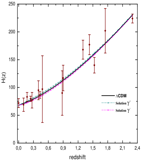
Figure 1: As an example, we show the Hubble parameter as a function of redshift for two models Capistrano . The model I is defined by the $\gamma^{(+)}$ and $\gamma^{(-)}$ solutions with the values for $\beta_{0}=2$ and $\eta_{0}=0.001$, the curves coincide with the curve from $\Lambda$CDM (solid line). Moreover, for the model II the curves are shown with $\gamma^{(+)}$ (triangles) and $\gamma^{(-)}$ (circles) solutions for the values $\beta_{0}=2$ and $\eta_{0}=0.25$. Error bar points were extracted from (cao, ) supplemented with additional data from (busca, ; zhai, ) at $H(z=2.3)$.

In order to do not jeopardize the nucleosynthesis, we use $|r_{nuc}=r(z\sim 10^{9})|\leqslant 10\%$ grande ; sola that gives a constraint $\beta_{0}\lesssim 0.465$. Moreover, from Eq.(17), we can write the deceleration parameter conveniently written in terms of the redshift $z$ as

$$q(z)=\frac{1}{H(z)}\frac{dH(z)}{dz}(1+z)-1\;.$$ (22)

Hence, we can write

$$q(z)=\frac{3}{2}\left[\frac{\Omega_{\;m}(1+z)^{3}+\gamma^{*}\Omega_{\;ext}(1+z)^{4-2\beta_{0}}e^{\mp\gamma(z)}}{\Omega_{\;m}(1+z)^{3}+\Omega_{\;ext}(1+z)^{4-2\beta_{0}}e^{\mp\gamma(z)}}\right]-1\;\;,$$ (23)

where $\gamma^{*}=\frac{1}{3}\left[4-2\beta_{0}\pm 2\sqrt{\frac{4\eta_{0}}{(1+z)^{4}}-3}\;\right]$.

Using the related value of $\beta_{0}$ for nucleosynthesis era, the baryon contribution $\Omega_{b}\mathrel{\mathop{\mathchar 58\relax}}=0.022\pm 0.00023$ and Cold dark matter contribution $0.1197\pm 0.0022$ with $68\%$C.L. Ade , we obtain the deceleration parameter $q\sim 0.535$ with the expected ratio $r\sim 0.1$. Moreover, for $\beta_{0}=1/2$ (that corresponds to the matter dominated era with $w=0$ in accordance with Eq.(21) ) and $\eta_{0}=0.001$, we obtain the predicted value $q=1/2$ expected for the matter domination and putting $\beta_{0}=1/2$ in Eq.(20) it converges to the value $r_{0}=3/7$. Actually, the same value for the deceleration parameter is obtained even considering the highest value of $\eta_{0}=0.5$. Moreover, taking Eq.(23) with the previous values for $\beta_{0}=1/2$ and $q=1/2$ related to matter-dominated era, we can obtain an estimative for the magnitude of the “equivalence redshift” $z_{e}$ given by

$$z_{e}=|\left(\frac{4}{3}|\eta_{0}|\right)^{(1/4)}-1|\;.$$ (24)

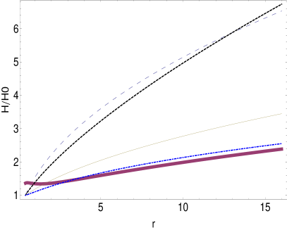
(a)

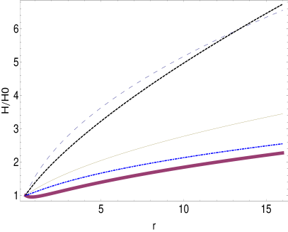
(b)

Figure 2: The relation of Hubble parameter to ratio $r$ raging from the input parameter $r_{0}=3/7$ to $r=15.4$ where is present the solutions of the model, including a XCDM-like solutions for $\pm\gamma=0$. The thin line mimics the $\Lambda$CDM model with $w=-1$, the thick dashed line mimics a quintessence model with $w=-0.73$. Phantom models with $w=-1.2$ are represented by the thick dotted-dashed line. The dashed lines and thick lines are solutions for $\pm\gamma\neq 0$.

In order to approximate the matter dominated era we know that the variation of the $\eta_{0}$ parameter has a constrained small value in the accelerated expansion where was found that $0\leq\eta_{0}\leq 0.5$ that gives the range $1\geq z_{e}\geq 0.09$. Interestingly, if we consider a tighter range for the width of transition, i.e., $0.01\leq\eta_{0}\leq 0.25$, we have $0.66\geq z_{e}\geq 0.24$ which means that the beginning of the “coincidence” happens in the end of the matter dominated era, since the value of $z_{e}$ matches the transition redshift from a deceleration to accelerated phase, as several different data sets indicate, e.g, $z_{t}=0.56^{+0.13}_{-0.10}$ as the latest Baryons Acoustic Oscillations/Cosmic Microwave Background (BAO/CMBR) + SNIa Giostri with MLCS2K2 light-curve fitter or using the SALT2 fitter $z_{t}=0.64^{+0.13}_{-0.07}$. This leads us to the interesting conclusion that the apparent “coincidence” began in the matter-dominated era and the current “coincidence” observed is far from being special.

It is important to point out that the apparent variation of the $\beta_{0}$ parameter is from its inner relation to the deceleration parameter $q$ and any change of $\beta_{0}$ is related to phase transitions in the universe. As previously commented, the current accelerated expansion (at $z=0$) regime can be obtained with $2\leq\beta_{0}\leq 3$ and with the expected $q_{0}<0$. In short, based on the fact that we have minima points such that $\beta_{0}<1/2$, the $\beta_{0}$ parameter can be constrained as $0.465\leq\beta_{0}\leq 3$ from nucleosynthesis until the present-day accelerated expansion regime.

In addition, we try to obtain more information on the evolving $r$ looking for a relation between Hubble parameter and the ratio $r$. At first, one can write the following relation

$$\dot{r}=\dot{H}\frac{dr}{dH}\;.$$ (25)

Starting from calculating the first derivative of the Friedman equation in Eq.(15) in terms of densities $\rho_{m}$ and $\rho_{ext}$, one can obtain

$$\dot{H}=\frac{\kappa^{2}}{6}\left((2\beta_{0}-4)\rho_{ext}\exp{(\pm\gamma)}-3\rho_{m}\pm\rho_{ext}\dot{\gamma}\frac{\exp{(\pm\gamma)}}{H}\right)\;.$$

After a long algebra, one can write

$$\dot{H}=-\frac{3}{2}\left[\frac{r+\Theta\exp{(\pm\gamma)}}{r+\exp{(\pm\gamma)}}\right]H^{2}\;.$$

Interestingly, if we consider a particular case (i.e, to mimic XCDM), one can set the term $\gamma=0$ and the appropriate correspondence $\beta_{0}=\frac{1}{2}\left(1-3w\right)$, where $w<-1/3$. So we have $\Theta=1+w$. Hence,

$$\dot{H}=-\frac{3}{2}\left[\frac{1+w+r}{r+1}\right]H^{2}\;,$$

which is the same equation obtained in (delcampo, ).

Moreover, the relation in Eq.(25) can be readily integrated and after a long algebra, one can write

$$H=H_{0}\left[\frac{r+\exp{(\pm\gamma)}}{r_{0}+\exp{(\pm\gamma)}}\right]^{-\frac{3}{2}\frac{1-\Theta}{(1-2\beta_{0})}}\left(\frac{r}{r_{0}}\right)^{-\frac{3}{2}\frac{(\Theta)}{(1-2\beta_{0})}}\;,$$

where the Hubble parameter $H$ is a function of $r$. The function $\Theta(r)$ is denoted by

$$\Theta(r)=\frac{1}{3}\left[(4-2\beta_{0})\pm 2\sqrt{4\eta_{0}\left(\frac{r}{r_{0}}\right)^{4/(2\beta_{0}-1)}-3}\right]\;,$$

with two signs $\Theta^{+}$ and $\Theta^{-}$. These two possibilities induce to four possible behaviors of $H(r)$ which we denote $H(r)^{+-},H(r)^{-+},H(r)^{++},H(r)^{--}$ as shown below.

$$H(r)^{+-} = H_{0}\left[\frac{r+\exp{(+\gamma)}}{r_{0}+\exp{(+\gamma)}}\right]^{-\frac{3}{2}\frac{1-\Theta^{-}}{(1-2\beta_{0})}}\left(\frac{r}{r_{0}}\right)^{-\frac{3}{2}\frac{(\Theta^{-})}{(1-2\beta_{0})}}\;$$

$$H(r)^{--} = H_{0}\left[\frac{r+\exp{(-\gamma)}}{r_{0}+\exp{(-\gamma)}}\right]^{-\frac{3}{2}\frac{1-\Theta^{-}}{(1-2\beta_{0})}}\left(\frac{r}{r_{0}}\right)^{-\frac{3}{2}\frac{(\Theta^{-})}{(1-2\beta_{0})}}\;$$

$$H(r)^{++} = H_{0}\left[\frac{r+\exp{(+\gamma)}}{r_{0}+\exp{(+\gamma)}}\right]^{-\frac{3}{2}\frac{1-\Theta^{+}}{(1-2\beta_{0})}}\left(\frac{r}{r_{0}}\right)^{-\frac{3}{2}\frac{(\Theta^{+})}{(1-2\beta_{0})}}\;$$

$$H(r)^{-+} = H_{0}\left[\frac{r+\exp{(-\gamma)}}{r_{0}+\exp{(-\gamma)}}\right]^{-\frac{3}{2}\frac{1-\Theta^{+}}{(1-2\beta_{0})}}\left(\frac{r}{r_{0}}\right)^{-\frac{3}{2}\frac{(\Theta^{+})}{(1-2\beta_{0})}}\;$$

In Fig.(2) we present some results of different models with an evolving Hubble parameter as the ratio $r$ increases (and the coincidence ceases to be). As a particular solution of our model, one can get the curves in fig.(2) that mimics XCDM, as previously commented. The thin line mimics the $\Lambda$CDM model with $w=-1$, the thick dashed line mimics a quintessence model with $w=-0.73$. Phantom models with $w=-1.2$ are represented by the thick dotted-dashed line. In the left panel, the dashed line and the thick line represent the functions $H(r)^{++}$ and $H(r)^{+-}$, respectively. In the right panel, the dashed line and the thick line represent the functions $H(r)^{-+}$ and $H(r)^{--}$, respectively.

We note that both left and right panels present a general similar behavior. Starting with $H(r)^{++}$ and $H(r)^{-+}$ one finds curves very close to a quintessence model. Moreover, the $H(r)^{+-}$ and $H(r)^{--}$ are close to phantom. The solution $H(r)^{+-}$ presents a smooth decaying at $r<1$ differently from $H(r)^{--}$ that mimics a more negative equation of state with $w=-1.3$ . It is worth noting to say that the evolution of $H(z)$ in terms of redshift was shown in (Capistrano, ) and the values of parameters $(\eta_{0}=0.25,\beta_{0}=2)$ passed through cosmokinetics tests confronted to observational data from (cao, ) based on observations of red-enveloped galaxies (stern, ) and BAO peaks (gaztanaga, ) being also supplemented with the observational data on Hubble parameter (OHD) and BAO in Ly$\alpha$ (busca, ; zhai, ) with $H(z=2.3)=(224\pm 8)km.s^{-1}.Mpc^{-1}$. As it may seem, the apparent coincidence is caused by the effect of extrinsic curvature on the dynamics of the universe mainly on the variation of the deceleration parameter.

IV Final remarks

Until recently the problem of classes of equivalence of manifolds defined by the same Riemann curvature, but with different topological properties, was ignored in general relativity because the Minkowski space-time, postulated as the ground state of gravitational field, is uniquely and well defined as a flat-plane manifold, characterized by the existence of Poincaré translations in all directions in all of its points. However, recent astrophysical experiments such as, e.g, WMAP, SDSS and Planck Mission, have shown that exists a small CC which explains the accelerated expansion within the so called $\Lambda$CDM paradigm. In this case, we no longer have the Minkowski space-time as a solution of Einstein’s equations, so that the ground state of the gravitational field, or equivalently the Minkowski standard of Riemann curvature set by Einstein is ambiguous: Either we have Minkowski without CC or else we have de Sitter space-times with CC. In order to solve that problem, the embedding between geometries has been revealed to be an appropriate underlying mechanism to obtain a gravitational theory and a possible way to get to a quantum-gravity theory QBW ; rostami ; jalal in the future. The relevant detail in Nash’s theorem is that it provides a mathematically sound and coordinate gauge free way to construct any Riemannian geometry, and in particular any space-time structures by a continuous sequence of infinitesimal perturbations along the extra dimensions of the bulk space generated by the extrinsic curvature. Due to its perturbative characteristics, Nash’s geometric smooth perturbative process can be an important principle to cosmological applications.

We focused our present work on the “new” CC problem commonly referred as coincidence problem on the values of the contributions of matter and the vacuum and the why they seem to have the same order. Motivated by the former geometrical dilemma on Riemann’s geometry, we studied the contribution of the extrinsic curvature as a dynamical quantity and its influence to the coincidence problem as we replace the CC contribution by the extrinsic one. It was shown that the coincidence problem can be at least alleviated with the presence of the extrinsic curvature. Interestingly, the $\beta_{0}$ parameter revealed to be very promising term since it is related to the magnitude of the declaration parameter $q$ and its small changes are related to the transition phases of the universe. It helped us to understand that the current coincidence ceases to be since it began close to the end of the matter dominated or even in the passage from the decelerated to accelerated regime, where we found the “equivalence” redshift around $0.66\geq z_{e}\geq 0.24$ compatible with the transition phase. Moreover, the parameter $\beta_{0}$ could be highly constrained as $0.465\leq\beta_{0}\leq 3$ from nucleosynthesis until the present-day accelerated expansion era showing how the ratio $r$ evolved to its present value $r_{0}=3/7$. An explicit relation of the ratio of the densities $r=\frac{\rho_{m}}{\rho_{ext}}$ to the Hubble parameter was obtained in order to understand more the dynamics on the ratio $r$. This analysis can be improved as the observational data of the ratio $r$ can be available in future observations.

References

- (1) N. Arkani-Hamed, S. Dimopoulos, G. Dvali, Phys. Lett. B, 429, 263, (1998).
- (2) L. Randall, R. Sundrum, Phys. Rev. Lett., 83, 3370, (1999).
- (3) L. Randall, R. Sundrum, Phys. Rev. Lett., 83, 4690, (1999).
- (4) S.H.H. Tye, I. Wasserman, Phys. Rev. Lett., 86, 1682, (2001).
- (5) S. Tsujikawa, M. Sami, R. Maartens, Phys. Rev. D, 70, 063525, (2004).
- (6) Z. Kakushhadze, Phys. Lett. B, 491, 317, (2000).
- (7) R. Maartens, Living Rev. Rel., 7, 7, (2004).
- (8) T. Shiromizu, K. Maeda, M. Sasaki, Phys. Rev. D, 62, 024012, (2000).
- (9) M. Heydari-Fard, H.R. Sepangi, Phys.Lett. B, 649, 1, (2007).
- (10) S. Jalalzadeh, M. Mehrnia, H.R. Sepangi, Class.Quant.Grav., 26, 155007, (2009).
- (11) M.D. Maia, N. Silva, M.C.B. Fernandes, JHEP, 047, 04, (2007).
- (12) T. Rostami, S. Jalalzadeh, Phys. Dark Univ., 9-10, 31, (2015).
- (13) S. Jalalzadeh, T. Rostami, Int. J. Mod. Phys. D, 24, 1550027, (2015).
- (14) M. Heydari-Fard, M. Shirazi, S. Jalalzadeh, H. R. Sepangi, Phys. Lett. B 640, 1, (2006).
- (15) J. Nash, Ann. Maths., 63, 20, (1956).
- (16) S.N. Gupta, Phys. Rev., 96, 6, (1954).
- (17) M.D Maia, A.J.S Capistrano, J.S. Alcaniz, E.M. Monte, Gen. Rel. Grav., 10, 2685, (2011).
- (18) S. Weinberg, Rev.Mod.Phys., 61, 1, (1989).
- (19) S. Weinberg, The Cosmological Constant Problems (Talk given at Dark Matter 2000, February, 2000), ArXiv:astro-ph/0005265.
- (20) I. Shapiro, J. Sóla, Phys. Lett. B, 475, 236, (2000).
- (21) I. Shapiro I., J. Sóla, Nuc. Phys. B (Proc. suppl.), 127, 71, (2004).
- (22) I. Shapiro I., Class. Quantum Grav., 25, 103001, (2008).
- (23) J. Bardeen, Phys. Rev. D, 31, 1792, (1985).
- (24) R. Geroch, Comunn. Math. Phys., 13, 180, (1969).
- (25) J. M. Stewart, M. Walker, Proc. Roy. Soc. (London), A341, 49 (1974).
- (26) R. Greene, Memoirs Amer. Math. Soc., 97, (1970).
- (27) B. Riemann (Translated by W. K. Clifford), Nature, 8, 114, 136, (1873).
- (28) J. Rosen, Rev. Mod. Phys., 37, (1965).
- (29) P. Szekeres, ll Nuovo Cimento A Series 10, 43, 4, (1966).
- (30) M.D. Maia, E.M. Monte, J.M.F. Maia, Phys. Lett. B, 585, 1-2, (2004).
- (31) N. Dalal, K. Abazajian, E. Jenkins, A.V. Manohar, Phys. Rev. Lett., 86, 1939, (2001).
- (32) J.S Alcaniz et al., Phys. Lett. B, 716, 165, (2012).
- (33) S. Del Campo, R. Herrera, D. Pavón, Phys. Rev. D, 78, 021302(R), (2008).
- (34) A.J.S Capistrano, Mon.Not.Roy.Astron.Soc., 448, 1232, (2015).
- (35) M.S. Turner, M. White, Phys.Rev.D56, 4439, (1997).
- (36) P.A.R. Ade et.al. (PLANCK Collaboration), Planck 2015 results. XIII. Cosmological parameters, ArXiv: 1502.01589.
- (37) S. Cao, Z.H. Zhu, N. Liang, AA, 529, A61, (2011).
- (38) N.G. Busca et al., AA, 552, A96, (2013).
- (39) Z.X. Zhai et al., Phys. Lett. B727, 8, (2013).
- (40) J. Grande, J. Solà, H. Štefancic, J. Phys. A, 40, 6787, (2007).
- (41) J. Solà, H. Štefancic, Phys. Lett.B, 624, 147, (2005).
- (42) R. Giostri et al., JCAP, 1203, 027, (2012).
- (43) D. Stern et al., JCAP, 02, 008, (2010).
- (44) E. Gaztañaga, A. Cabré, L. Hui, Mon.Not.Roy.Astron.Soc., 399, 1663, (2009).