Calculation of expectation values of operators in the Complex Scaling method

Abstract

The complex scaling method (CSM) provides with a way to obtain resonance parameters of particle unstable states by rotating the coordinates and momenta of the original Hamiltonian. It is convenient to use an L² integrable basis to resolve the complex rotated or complex scaled Hamiltonian H_θ, with $\theta$ being the angle of rotation in the complex energy plane. Within the CSM, resonance and scattering solutions do not exhibit an outgoing or scattering wave asymptotic behavior, but rather have decaying asymptotics. One of the consequences is that, expectation values of operators in a resonance or scattering complex scaled solution are calculated by complex rotating the operators. In this work we are exploring applications of the CSM on calculations of expectation values of quantum mechanical operators by retrieving the Gamow asymptotic character of the decaying state and calculating hence the expectation value using the unrotated operator. The test cases involve a schematic two-body Gaussian model and also applications using realistic interactions.

I Introduction

When a nucleus or any other quantum mechanical system is in a metastable state with positive energy and decays to a more stable configuration by emitting massive particles or photons, the state is widely known as a resonance. For the resonance to be fully characterized one needs to know the positive energy above the associated threshold, which can be denoted as E_r, and also a quantity that would be related to the time that is takes for the resonance to decay to the more stable configuration. The latter is known as the width $\Gamma$ of the resonance. E_r and $\Gamma$ uniquely define the resonance and they are called resonance parameters.

Resonances appear in reaction experiments, manifested as enhanced “bumps” in the measured cross-sections. In nuclear physics, resonance parameters have been extracted by fitting the Thomas-Lane formulas Lane and Thomas (1958) to the data, as for example in the compilation of light nuclei in Tilley et al. (1992). This process is known as phenomenological R-matrix and has been the workhorse for data evaluation and determination of resonance parameters. There also exists a wealth of microscopic methods to solve the nuclear many-body problem and obtain resonance parameters. At this point one needs to distinguish the phenomenological R-matrix for fitting the data, to the calculable R-matrix Descouvemont and Baye (2010); Thompson (1988).

The calculable R-matrix provides with a numerical foundation for solving the scattering problem by assuming a partition of the space into internal (bound states regime) and external (scattering regime) and using a matching of the solutions and appropriate boundary conditions at infinity. It has been applied for evaluation of scattering observables and resonances with both phenomenological Descouvemont and Baye (2010); Thompson (1988) and also realistic nucleon-nucleon interactions Quaglioni and Navrátil (2009). There has been a lot of work for describing nuclear physics phenomena with positive energies and the effort cannot be captured in this work, howewer it needs to be mentioned that another basic numerical tool to study reaction mechanisms is the so-called continuum discretized coupled channel (CDCC) approach, especially for multi-channel reactions and reactions that involve reactions of nuclei with fragile radioactive beams Austern et al. (1987); Thompson and Nunes (2009).

The last decade there is a revival of methods that are developed in the complex energy plane and provide a solid theoretical framework towards the unification of structure and reaction aspects of nuclei. Examples are calculations in the Berggren basis Michel et al. (2009); Id Betan et al. (2003); Papadimitriou et al. (2013); Hagen and Michel (2012); Lundmark et al. (2015); Jaganathen et al. (2014) which is a complex single particle (s.p.) basis that utilizes extended completeness relations Berggren (1968) and unifies resonant and non resonant continuum degrees of freedom.

A resonant state or Gamow state or complex pole of the S-matrix, is a state regular at the origin that satisfies outgoing boundary conditions at infinity. In this sense, resonant states cannot be described by Hermitian Quantum Mechanics (QM) which deal with wavefunctions that vanish at large distances. However, since very soon the usefulness of the resonant states was realized for the theoretical description of time dependent processes (e.g. radioactive decays) and Open Quantum Systems (OQSs) Okołowicz et al. (2003), solid mathematical foundations were developed Bottino et al. (1962); Aguilar and Combes (1971); *abc2; Simon (1972); de la Madrid (2004); Civitarese and Gadella (2004) in the framework of non-Hermitian QM and also advances in numerical techniques and non-Hermitian diagonalizers were called for Milfeld and Moiseyev (1986); Santra and Cederbaum (2002); Mizusaki et al. (2014); Vecharynski et al. (2015).

Studying reactions in the complex energy plane can have some attractive advantages. It has been observed that even in the phenomenological R-matrix case, it is beneficial to perform a continuation of the S-matrix in the complex energy plane in order to determine more reliably resonance parameters Csótó and Hale (1997). At first glance the complex energy would seem unnatural since reactions take place on the real energy axis. The formulation on the complex energy, however, offers a mathematical getaway that alleviates some, difficult to tackle, problems on the real axis and then an analytical continuation on the real axis takes place in order to calculate scattering quantities.

On the real axis and on the configuration space it is known that boundary conditions quickly become complicated by increasing the number of reactive particles and in the case of three charged particles the asymptotic is not even known in closed form. Such boundary conditions are not appearing in momentum space, but then one deals with singularities which are treated by calculating the resolvent in the complex energy plane by going over the singularity by small finite radii Kamada et al. (2003); Uzu et al. (2003). This technique is widely known as complex energy method and was recently employed successfully for describing reactions above four-body breakup threshold with realistic interactions Deltuva and Fonseca (2014a); *deltuva2 and also for calculations on the lattice Rupak and Lee (2013). The analytical continuation on the real axis is taken after extrapolations of the radius, that goes over the singularity, to zero.

The other complex energy alternative is based on a rotation of coordinates and momenta of the Hamiltonian which leads in bound state like boundary conditions for the description of scattering. The work was originated by Nuttall and Cohen Nuttall and Cohen (1969), as a way of solving the purely scattering many-body problem for energies above the break-up threshold to obtain scattering amplitudes without imposing many-body scattering boundary conditions. It was shown to be successful for both short range and long range potentials Rescigno et al. (1997); Kruppa et al. (2007); Kikuchi et al. (2011), for mean field calculations Shi et al. (2014), for scattering calculations above the four body break-up threshold Lazauskas (2012) and recently also facilitated modern nuclear forces Lazauskas (2015); Papadimitriou and Vary (2015a, b). This complex energy formalism appears with different names and flavors in bibliography such as complex-coordinate method Moiseyev and Hirschfelder (1988); Nuttall and Cohen (1969) or complex scaled Lippmann-Schwinger (CSLS) method Kruppa et al. (2007); Kikuchi et al. (2011). In our work we are using the uniform complex rotation of coordinates and momenta which will give rise to a complex eigenvalue problem and in all the following this will be denoted as Complex Scaling Method (CSM) Moiseyev (1998); Ho (1983) which is also the most widely known name. In this case the analytical continuation on the real axis and the connection with real energy scattering observables is done through the calculation of the complex scaled Green’s operator that is used for the evaluation of the continuum level density.

Within the CSM, one is able to describe resonances naturally by calculating the complex eigenstates of a complex symmetric non-Hermitian Hamiltonian matrix. The wavefunctions $\Phi_{\theta}$, which are a linear combination of $L^{2}$ integrable basis states, do not have the asymptotic behavior that would characterize a resonant state and they fall-off at large distances. It is known that in order to obtain the Gamow or outgoing character of the CSM wavefunction one needs to perform the backrotation operation: $\Phi$ = U$(\theta)$^-1$\Phi_{\theta}$. The backrotation, however, is shown to be very unstable and it belongs in the category of ill-posed inverse problems.

There are ill-posed inverse problems within the low-energy nuclear physics field that have been tackled through regularization process. The inversion of the Laplace Transform faced in calculations of the Trento group for electromagnetic response functions was treated with the Lorentz Inverse Transform ) method Efros et al. (1994), while for calculations of nuclear responses within the Argonne’s imaginary time Quantum Monte Carlo (QMC) methods, the inversion of the imaginary time Euclidean response is stabilized via maximum entropy techniques (MET) Lovato et al. (2015). In QMC calculations of the Seattle-Warsaw groups, the spectral weight function which is calculated by inversion of the Green’s function, is also regularized by using the MET Magierski et al. (2009); Magierski and Wlazłowski (2012) or by singular value decomposition (SVD) Magierski and Wlazłowski (2012). Coming back to the CSM and the backrotation inverse problem, the regularization solution was proposed in Kruppa et al. (2014), it is known as Tikhonov regularization Fu et al. (2009); Tikhonov (1963); Tikhonov and Goncharsky (1987) and results in retrieving a meaningful Gamow state from the complex scaled solutions.

In this work we will apply the Tikhonov regularization technique for the backrotation of the complex scaled wavefunction and we will calculate expectation values of the radius and dipole operators. We will study the behavior of the backrotated wavefunctions and check the stability of the expectation values on the regularization parameter. We will apply our techniques to a schematic 3D Gaussian problem Csótó et al. (1990); Myo et al. (2014); Baye (2015) which supports bound states and resonances. We will also calculate the scattering phase shifts of the Gaussian model and deduce from them resonance parameters using R-matrix formulas. Having simultaneously the resonance parameters from the diagonalization of the complex scaled Hamiltonian we will study the limits of applicability of traditional R-matrix formulas, especially when the resonance has a large width. Finally we will present applications of the Tikhonov technique for the case of the deuteron system and study the expectation value of the dipole operator for the transition from the ³S₁-³D₁ coupled channel bound ground state (g.s.) to the ³P₁ continuum states and conclude with perspectives and future plans.

II The CSM

We will briefly mention the basic aspects of the CSM and also refer the reader to Moiseyev (1998); Ho (1983). The CSM is mathematically based on the Aguilar-Balslev-Combes (ABC) theorem Aguilar and Combes (1971); *abc2. A resonance can be revealed in the spectrum of the original Hamiltonian once the momenta and coordinates of the latter are uniformly rotated in the complex energy plane. The ABC theorem then states that the resonant states of the original Hamiltonian are invariant and the non-resonant scattering states are rotated and distributed on a 2$\theta$ ray that cuts the complex energy plane with a corresponding threshold being the rotation point. Within the CSM, a resonant state behaves asymptotically as a bound state (see also Fig.1), which implies that the description of resonances does not require special boundary conditions at infinity and their description adopting an L² integrable basis is sufficient.

The Hamiltonian is transformed under the action of the non unitary complex scaling operator U$(\theta)$ as:

$$H(\theta,r)=U(\theta)H(r)U(\theta)^{-1},$$ (1)

where we have assumed for simplicity that the Hamiltonian depends only on the coordinate r and U$(\theta)$ has the following property when acting on a state:

$$U(\theta)\Phi(r)=e^{\frac{3}{2}if\theta}\Phi(re^{i\theta})$$ (2)

with $f$ = 1 for a two-body system. CSM has the flexibility to be adopted to the coordinate system one uses to describe a particular nucleus, hence the degrees of freedom (or f in (2)) is usually larger than one e.g. for multi-cluster systems. One of the ways to solve the problem governed by the Hamiltonian in Eq.(1) is the expansion in a complete basis. Any L² basis could be employed for this purpose, such as the Harmonic Oscillator (HO) basis, Slater basis Kruppa et al. (2014),tempered Gaussian basis Arai et al. (2001), basis defined on a grid such as Lagrange mesh Baye (2015), Discrete Variable Representation basis Lill et al. (1986) etc. We are adopting for the time being the HO basis characterized by a length parameter $b$, without being restrictive to other more flexible basis and we end up with a complex symmetric eigenvalue problem:

$$H_{\theta}\Phi_{\theta}=E_{\theta}\Phi_{\theta}.$$ (3)

III Computations

III.1 Backrotation, expectation values of operators and phase-shifts with a schematic potential

III.1.1 Backrotation of CSM wavefunction

We start our calculations by considering a schematic Hamiltonian $H=-\frac{\hbar^{2}}{2\mu}\nabla^{2}+V$ with the potential consisting of two Gaussian form factors, one attractive and one repulsive:

$$V(r)=-8.0e^{-0.16r^{2}}+4.0e^{-0.04r^{2}}$$ (4)

and also working in a system of units where $\hbar$ = 1, $b$=1, $\mu$ = 1. It is worth noting that this potential was employed for first time in calculations for the exploration of the direct backrotation and how one could minimize errors associated with it in Csótó et al. (1990) and later on for CSM calculations of the complex scaled Green operator Homma et al. (1997); Myo et al. (1998); Odsuren et al. (2014). It also provides with a testing bed for other methods as well Baye (2015).

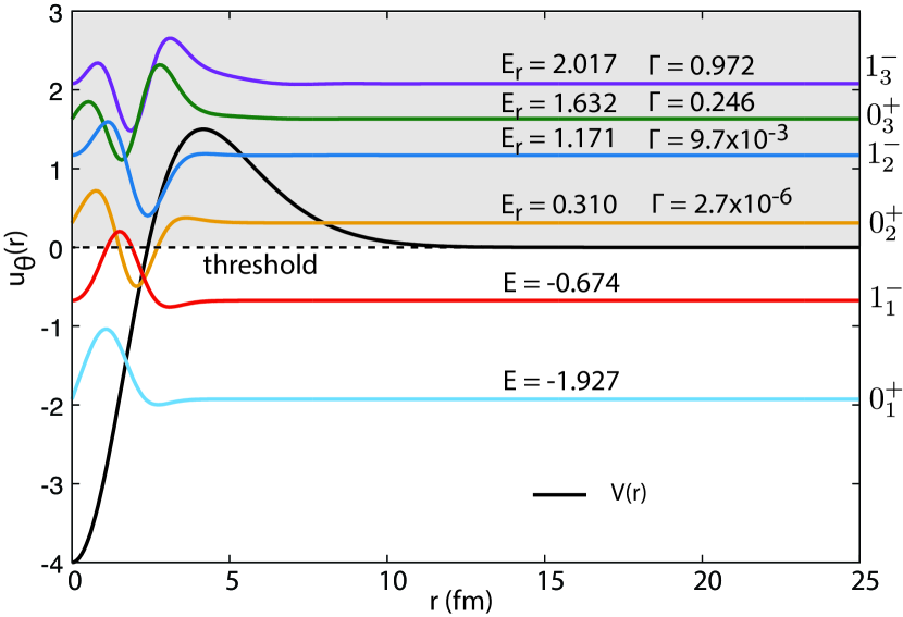
Figure 1: (Color online) Resonant eigenvalues and radial wavefunctions of the complex scaled schematic Gaussian Hamiltonian. The gray area denotes the positive energy part of the spectrum above threshold. Even though the last four states are above threshold, their radial dependence resembles the one of a bound state. The energies and widths are in MeV.

For the Hamiltonian in Eg.(4) the transformation (1) implies a uniform rotation of the coordinate as $r$ $\to$ $re^{i\theta}$ and momentum $p$ $\to$ $pe^{-i\theta}$. The kinetic energy becomes $\nabla^{2}$ $\to$ $\nabla^{2}e^{-2i\theta}$ and for the local potential we just have to scale the coordinate, so basically $r^{2}$ $\to$ $r^{2}e^{2i\theta}$. The solution is assumed to have the form (5) and the complex coefficients are determined by solving the non-Hermitian complex symmetric eigenvalue problem. In Fig.1 we gather some of the resonant solutions that the potential supports for the $\ell$=0,1 states for a basis size of N=30 HO radial nodes and a rotation angle $\theta$ = 0.35 radians. The resonant states depicted are invariant with respect to changes in $\theta$ and convergence was tested as a function of both the basis size and $\theta$. For a range of rotation angles up to $\theta$ = 0.6 radians and for N=30 the real and imaginary part of the resonant states are unchanged up to the sixth significant digit.

We notice of course that even though the resonant solutions above the threshold are all complex with non-zero widths, their radial dependence is reminiscent of a bound state. This is to be expected since the radial wavefunctions are expanded in an L² basis as:

$$u_{\theta}(r)=\sum_{n=1}^{N}C_{n}^{\theta}\phi_{n}(r)$$ (5)

where the expansion coefficients are the complex eigenvectors of the H_θ diagonalization and $\phi_{n}(r)$ in our case are the spherical HO radial basis functions. The radial wavefunctions have both real and imaginary parts because of the complex nature of the C^θ coefficients.

In order to obtain the Gamow character of the radial wavefunction u(r), as noted earlier, the backrotation transformation $U(\theta)^{-1}$ has to be applied on the CSM solution. In the case of the two-body problem and according to (2) that would constitute to the following transformation:

$$u(r)=e^{-\frac{3}{2}i\theta}\sum_{n=1}^{N}C_{n}^{\theta}\phi_{n}(re^{-i\theta}).$$ (6)

As it was shown in Kruppa et al. (2014) and also presented here in Fig.2, the direct backrotation is very unstable and retrieving the Gamow character of the wavefunction in this way is not possible. The source of the problem is two-fold. First, the expansion coefficients contain errors which are magnified in the process of the inversion. Second and actually the main source of the instability is that the HO backrotated basis functions exhibit a very large amplitude oscillatory behavior when increasing the back rotation angle $\theta$. This is exactly what is depicted in Fig.2 for the backrotation of the broad 1${}_{3}^{-}$ resonant state. Eventually the oscillations diminish for large distances, but at intermediate distances we observe very large amplitudes. This behavior of the complex scaled HO basis functions was the reason in Hagen et al. (2004) the authors worked in momentum space and adopted the contour deformation method for solving a complex momentum T-matrix equation. We also note that in a recent work of the CSM with realistic potentials Papadimitriou and Vary (2015a, b) the backrotation of HO basis functions did not cause any problem since, due to the short range nature of the nucleon-nucleon force, the complex scaled matrix elements were all converged.

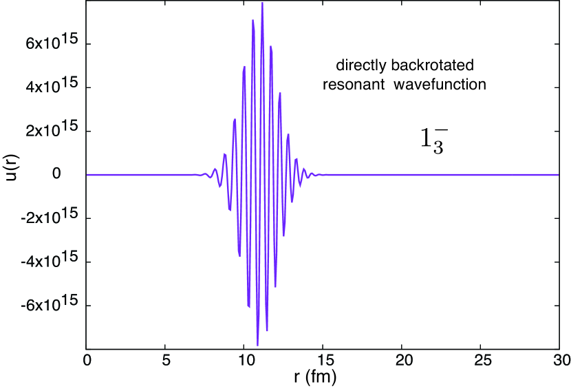
Figure 2: (Color online) Real part of the backrotated 1${}_{3}^{-}$ resonant state for $\theta$=0.35 rad and N=30. The subscript $\theta$ was dropped to differentiate from the CSM $u_{\theta}(r)$ solution.

At this point we will employ the Tikhonov regularization technique Kruppa et al. (2014); Fu et al. (2009). The recipe that is followed was used for first time in the context of CSM in Kruppa et al. (2014) and consists of three steps. Initially the function that needs to be backrotated is mapped onto the interval (-$\infty$,+$\infty$) through the transformation:

$$f_{\theta}(x)=u_{\theta}(r_{0}e^{-x}),$$ (7)

where u_θ is defined in Eq.(5) and $r_{0}$ = 1fm. The parameter $r_{0}$ serves the role of making variable $x$, as we will see below, dimensionless. Then Eq.(7) is Fourier transformed to obtain the:

$$u_{\theta}(\xi)=\frac{1}{\sqrt{2\pi}}\int_{-\infty}^{\infty}e^{-ix\xi}f_{\theta}(x)dx.$$ (8)

Finally, the regularized backrotated wavefunction is computed as:

$$u^{reg}(x+iy)=\frac{1}{\sqrt{2\pi}}\int_{-\infty}^{\infty}e^{-i(x+iy)\xi}$$

$$\times\frac{u_{\theta}(\xi)}{1+\kappa e^{-2y\xi}}d\xi,$$ (9)

where $x$ = $\ln(r/r_{0})$, y = $\theta$ and as we mentioned already $x$ and also $\xi$ are dimensionless quantities. The parameter $\kappa$ in Eq.(III.1.1) is the Tikhonov parameter which controls the smoothing of the backrotated wavefunction or the amount of regularization of the inverse problem of backrotation in CSM.

In Fig.3 we present the backrotated regularized $1_{3}^{-}$ wavefunction for several values of the parameter $\kappa$ and for comparison we also include the CSM $1_{3}^{-}$ wavefunction.

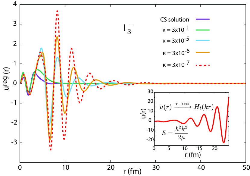
Figure 3: (Color online) Real parts of the reconstructed Gamow states for the 1${}_{3}^{-}$ resonant state. Several states corresponding to a different regularization parameter are shown. In the inset it is shown the true $1^{-}_{3}$ resonant solution which is regular at the origin and has a pure outgoing behavior Vertse et al. (1982).

We notice that depending on the regularization parameter $\kappa$ we obtain different Gamow states. In practice a CSM solution once backrotated via the Tikhonov method will generate an infinite number of Gamow states, since the parameter $\kappa$ can take any positive value. The wavefunctions are not observables so this feature is not necessarily a problem, but what we will investigate later is what the impact of the parameter $\kappa$ and of the form of the Gamow function on an observable.

Another feature that we observe is that the regularized wavefunctions do not exhibit the large amplitudes that we find in Fig.2. We see that for different values of the parameter $\kappa$ what is changing is basically the asymptotic behavior of the backrotated wavefunction. A large parameter $\kappa$ is shown to over-regulate the backrotated wavefunction and the form looks similar to the CSM one e.g. for $\kappa$ = 3$\times$10^-1. For distances r $<$ 3 fm (inside the potential well) the CSM wavefunction and the regularized backrotated wavefunctions look almost identical. For larger distances the regularized solutions are reminiscent of the behavior of an outgoing wave with an increasing amplitude for some distance outside the potential “lip” but with decaying amplitudes at larger distances. By backrotating hence the CSM solutions, the Gamow character of the resonant state being an outgoing wave at large distances is not fully retrieved. It is however interesting that for distances up to r $\sim$ 10 fm the behavior is more or else the expected one, namely a bound-state like formation inside the potential well and an outgoing wave just outside the well. It remains to be seen how observables will be affected once we will use the regularized backrotated states for the calculation of the expectation values. In the inset of Fig.3 we are showing the behavior of the true Gamow solution with a complex energy $E=2.017-i\frac{0.972}{2}$MeV, which was calculated by integrating the Shrödinger equation subjected to pure outgoing boundary conditions Vertse et al. (1982).

III.1.2 Calculations of the root mean square radius

Calculating an operator in a resonant state, as the one depicted in the inset of Fig.3, will lead in divergent matrix elements and the $r^{2}$ operator is not an exception. Techniques such as the exterior complex scaling Gyarmati and Vertse (1971) or Zel’dovich regularization Zel’dovich (1960) are employed for the calculation of integrals. In a recent work for the description of rotational bands in ⁸Be, expectation values of transition operators in the continuum were calculated by adopting the Zel’dovich prescription Garrido et al. (2013), whereas in GSM for example Michel et al. (2009) diverging integrals are computed though the exterior complex scaling.

In the case of CSM, since the resonant state is always behaving as a bound state the divergence is not appearing (see Table 1). One may say that due to the discretization of the continuum in the HO basis, the integral for the $r^{2}$ calculation is regulated by the fixed b and fixed N of the HO truncation and when one is using the Gamow backrotated solutions the integral is regulated via the Tikhonov method. Before continuing the discussion and applications of the backrotated wavefunctions, let us mention that the expectation value of an observable in a resonant state above threshold will always have an imaginary part as we will notice for the rms radius. It was explained by Berggren that the physical interpretation of the imaginary part of the operator is related to the uncertainty in the determination of its mean value Berggren (1996).

We saw that the Hamiltonian operator in CSM is transformed under (1). It is then expected that any quantum mechanical operator $\hat{O}$ will be transformed as:

$$\hat{O}(\theta)=U(\theta)\hat{O}U(\theta)^{-1},$$ (10)

as for example in ab-initio calculations of the dipole operator Horiuchi et al. (2012) or in benchmark CSM calculations Kruppa et al. (2014); Masui et al. (2014). In order to calculate its expectation value, one could use the transformed operator and calculate its expectation value between CSM solutions or calculate the expectation value of the bare operator but using the backrotated Gamow states. Now that we have obtained the regularized backrotated solutions for several Tikhonov parameters we will calculate the root mean square (rms) expectation value of the radius square operator $r^{2}$. We will perform our calculations for the unrotated bare $r^{2}$ operator in the broad $1_{3}^{-}$ resonant state using the wavefunctions that are shown in Fig.3 and the expectation value of the complex scaled operator $r_{\theta}^{2}\,=\,U_{\theta}r^{2}U_{\theta}^{-1}\,=\,e^{2i\theta}r^{2}$ will be used as a benchmark.

For the calculation we will use a large basis spanned by N=30 HO states so as to assure that $\langle r^{2}_{\theta}\rangle$ is fully converged as a function of basis states and as a function of $\theta$. For the rms radii calculations of the $1_{3}^{-}$ resonant state we used a value of $\theta$ = 0.4 rad. The state is revealed at an angle $\theta$ $\sim$ 0.23 rad in the complex energy plane and for values of $\theta$ = 0.35 and larger and for the size of the basis N=30 the radii have already converged up to the fourth significant digit as we present in Table 1.

Table 1: Dependence of the rms of the expectation value of the $r^{2}$ operator in the $1_{3}^{-}$ resonant state on the rotation angle $\theta$ for a basis of N=30 HO states. Both the real and imaginary parts are shown and the radius is expresed as $\langle r^{2}\rangle^{1/2}=(\Re(\langle r^{2}\rangle^{1/2}),\Im(\langle r^{2}\rangle^{1/2}))$.

$\theta$ (rad)	$\langle r^{2}\rangle^{\frac{1}{2}}$ (fm)
0.2	(3.693, 1.763)
0.3	(3.227, 1.398)
0.4	(3.220, 1.393)
0.5	(3.220, 1.393)
0.6	(3.220, 1.393)
0.7	(3.220, 1.393)

In Table 2 we gather the results for the rms expectation value of the $r^{2}$ operator for several renormalization parameters $\kappa$. The tilde symbol implies that conjugation does not affect the radial parts of the wavefunctions and stems from the fact that the solutions of the complex scaled Hamiltonian do not satisfy the usual inner product but rather the generalized c-product Moiseyev (1998). It is worth noting that the same holds for the backrotated regularized solutions since they are also not part of the Hilbert space and they do satisfy the generalized c-product.

Table 2: Calculations of the rms of the expectation value of the $r^{2}$ operator in the regularized backrotated Gamow states. Calculations correspond to N=30 and $\theta$ = 0.4.

$\kappa$	$\langle\widetilde{u^{reg}(r)}|r^{2}|u^{reg}(r)\rangle^{\frac{1}{2}}$ (fm)
3$\times$10-1	(4.36348, 0.80081)
3$\times$10-3	(3.24315, 1.34967)
3$\times$10-4	(3.21818, 1.39037)
3$\times$10-5	(3.22016, 1.39346)
3$\times$10-6	(3.22010, 1.39341)
3$\times$10-7	(3.22009, 1.39345)
3$\times$10-8	(3.22005, 1.39359)
3$\times$10-9	(3.22018, 1.39323)
3$\times$10-10	(3.22003, 1.39456)
$\langle\widetilde{u_{\theta}(r)}|e^{2i\theta}r^{2}|u_{\theta}(r)\rangle^{\frac{1}{2}}$	(3.22008, 1.39351)

For values of $\kappa$ smaller than 3$\times$10^-5 a plateau of rms radii starts to appear and the results coincide up to the fourth significant digit with the benchmark value of the CSM $r^{2}$ operator. For values larger than 3$\times$10^-4 the result is deteriorating since then as was also shown in Fig.2 there is an over-regulation of the backrotated Gamow state. Overall, for a range of parameters $\kappa$ the rms radius computed from the backrotated wavefunctions is coinciding with the expectation value of the complex rotated operator and the fact that the backrotated states go to zero for large distances, does not really affect the expectation value of the radius operator. We can safely claim then that the Tikhonov backrotation produces a Gamow function which does not require extra care for treating the asymptotic distance divergence of a typical Gamow state, but at the same time reproduces the results that would be obtained using the exact outgoing solution of the Shrödinger equation.

III.1.3 Calculations of the dipole strength function.

The calculation of the dipole strength function constitutes the calculation of the expectation value of the dipole operator between two different states. The so called dipole transition is allowed between states with opposite parity and that differ by one unit of angular momentum. Testing the Tikhonov regularization for such an observable is a more stringent test since the transition will involve an ensemble of states which will be backrotated and not a single state. The CSM allows to conveniently calculate the strength function via the complex scaled Green’s function and by exploiting the completeness relation of the CSM resonant and and non-resonant scattering solutions. The completeness relationship in CSM reassures that the many-body spectrum of the CSM Hamiltonian (1) which contains resonant and non-resonant scattering states form a complete set Giraud and Katō (2003) and allows to separate contributions of each element in computations of strength functions, phase-shifts and cross-sections Myo et al. (2014). The completeness of the CSM spectrum is formally identical to the Berggren completeness Berggren (1968) relation which was also utilized in the Gamow Shell Model (GSM) Michel et al. (2009).

The dipole strength function $\mathcal{S}(E)$ in CSM then is given by the following formula:

$$\mathcal{S}(E)=-\frac{1}{\pi}\sum_{\nu=1}^{N}Im\frac{\langle\widetilde{u_{\theta}^{i}(r)}|\hat{O}(\theta)|u_{\theta}^{\nu}(r)\rangle\langle\widetilde{u_{\theta}^{\nu}(r)}|\hat{O}^{\dagger}(\theta)|u_{\theta}^{i}(r)\rangle}{E-E_{\nu}^{\theta}},$$ (11)

where the indexes i and $\nu$ denote the initial and final states between which the transition occurs, $E$ is the excitation energy above threshold, $E_{\nu}$ are the complex eigenstates of the CSM Hamiltonian which we do not distinguish at this point if they are resonant or non-resonant continuum states and $\nu$ then denotes the number of states we use for discretizing the continuum, hence it is equal to the number N of HO states we use in the basis. Usually, for calculations that take place on the real energy axis, the number $\nu$ is also referred to as pseudostates for the fact that one describes the continuum in a bound state method spirit. The operator $\hat{O}$ in our case is the dipole operator $\hat{O}$ = $\frac{4\pi}{3}rY_{0}^{1}$ which is transformed as $\hat{O}(\theta)$ = $\hat{O}$$e^{i\theta}$ and also $\hat{O}^{\dagger}(\theta)$ = $\hat{O}^{\dagger}$$e^{i\theta}$.

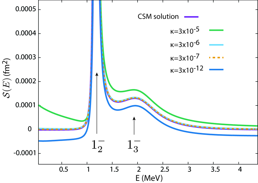
Figure 4: (Color online) Response function for the transition $0^{+}$ bound ground state $\to$ $1^{-}$ states in the continuum. The 1^- CSM solutions were all backrotated using the Tikhonov method. For several Tikhonov parameters $\kappa$ we compare the results against the CSM solution. The arrows denote the positions of the resonances (see also Fig.1).

As we did for the radius operator, we backrotate in (11) each one of the CSM solutions that are involved in the summation. We then calculate the strength as:

$$\mathcal{S}(E)=-\frac{1}{\pi}\sum_{\nu=1}^{N}Im\frac{\langle\widetilde{u_{reg}^{i}(r)}|\hat{O}|u_{reg}^{\nu}(r)\rangle\langle\widetilde{u_{reg}^{\nu}(r)}|\hat{O}^{\dagger}|u_{reg}^{i}(r)\rangle}{E-E_{\nu}^{\theta}},$$ (12)

using the bare dipole operator and not the $\hat{O}(\theta)$ one. We gather our results on Fig.4. As we see, for a range of Tikhonov parameters the strength function (12) calculated with the regularized Gamow states is identical to the strength function using formula (11) and a similar situation was also encountered in rms radius calculation. As a matter of fact, in Kruppa et al. (2014) a criterion that eliminates too low and too large values of $\kappa$ was established, confirming that there is a plateau of regularization parameters for which results are converged. This is important to know as we may not have an “exact” reference curve to our disposal. Furthermore, we may also conclude that the regularized backrotated functions also form a complete set which includes resonant and non-resonant backrotated states.

The problem of this chapter consisted of studying the resonant features of two particles interacting in a potential well, which is very similar with the way s.p. basis is generated for certain problems. We have seen basis generating potentials of Woods-Saxon type Vertse et al. (1982); Michel et al. (2009) or once again Gaussian potentials (e.g. KKNN Kanada et al. (1979)) that are basically effective forces imitating the interaction of a target with a single projectile. The possibility of obtaining a basis after backrotating CSM solutions could be considered and it worths to check if the set of backrotated states forms an orthogonal set.

In Fig.5 we plot the overlaps of the solutions for the $1^{-}$ backrotated states.

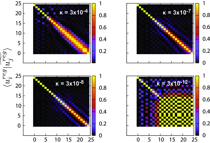
Figure 5: (Color online) Overlaps of the regularized backrotated $1^{-}$ states of the Gaussian schematic model for N=25 and $\theta$ = 0.3.

We see that for $\kappa$ = 3$\times$10^-7 and $\kappa$ = 3$\times$10^-8, that also belong in the plateau of parameters that provide excellent agreement with the comparisons against the CSM solutions and the CSM operators, most of the overlaps are zero but the matrix is not strictly unity. The similarity with the unity matrix is worse for other Tikhonov parameters. In general the regularized backrotated states are not orthogonal and if one could find a way to utilize them in a basis expansion method that would lead to a generalized diagonalization problem, with the calculation of the norm kernel being a necessity.

III.1.4 Phase shifts and widths.

We make a small parenthesis from studying the Tikhonov regularization in more realistic cases and we will compute the scattering phase shifts produced by the schematic model. Within the CSM the resonance parameters are determined as the eigenstates of the CSM Hamiltonian matrix which are stationary with respect to variations of the rotation angle. An eigenstate then with complex energy $E=E_{r}-i\frac{\Gamma}{2}$ will fully characterize the resonance. Of course, resonance parameters can be also conveniently calculated using techniques on the real energy axis. One of the most common ways to calculate resonance parameters on the real-axis is by using the inflection criterion for the scattering phase shifts Thompson and Nunes (2009). The position of the resonance $E_{r}$ then is computed from the derivative of the phase-shift at the point that this derivative is maximum and the widths are obtained using the formula:

$$\Gamma=\frac{2}{d\delta(E)/dE}\big{|}_{E=E_{r}}.$$ (13)

In CSM one can also calculate phase-shifts and then applying the inflection criterion formula we could see under which conditions are agreeing with each other.

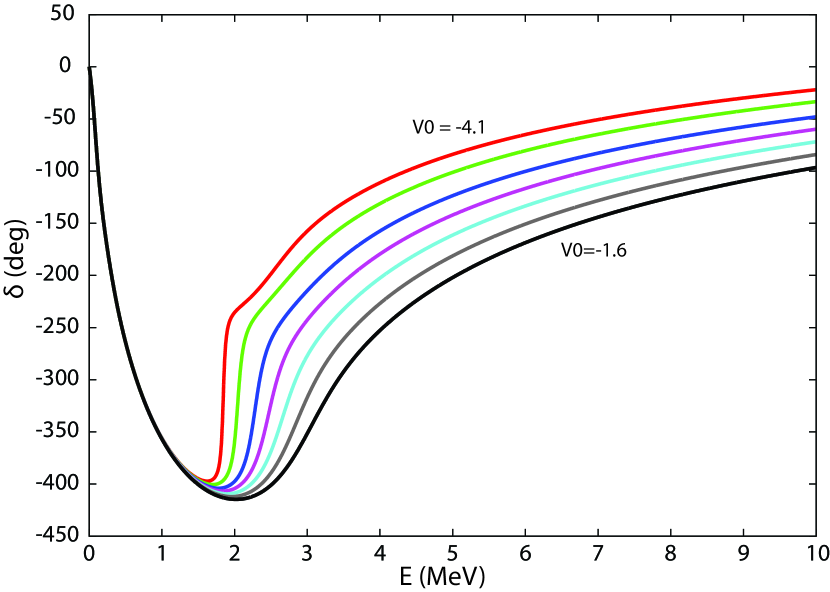
Figure 6: (Color online) Elastic scattering phase shifts for the schematic Gaussian potential as a function of the potential depth. The inflection criterion is applied to the phase shifts in order to deduce resonance parameters. See also Table 3.

We calculate the phase shifts through the complex scaled continuum level density (CLD). The complex scaled CLD is defined as Suzuki et al. (2005):

$$\Delta^{\theta}(E)=-\frac{1}{\pi}Im\int d{\bf r}\langle{\bf r}|\frac{1}{E-H_{\theta}}-\frac{1}{E-H_{\theta}^{0}}|{\bf r^{\prime}}\rangle.$$ (14)

and

$$\delta(E)=\int_{0}^{E}\Delta^{\theta}(E)dE.$$ (15)

In (14) $H_{\theta}$ is the CSM interacting Hamiltonian whereas $H_{\theta}^{0}$ is the CSM kinetic energy. We should note that in (14) all the eigenvalues of the complex rotated interacting and asymptotic Hamiltonian are needed, nevertheless investigations on truncations of the number eigenvalues and the impact they have on the phase-shifts are underway. By calculating the CLD we could already determine resonance parameters because of its relation to the S-matrix and resonances appear as pronounced peaks on the CLD spectrum. The authors in Kruppa (1998); Arai and Kruppa (1999); Kruppa and Arai (1999) showed that resonance parameters can be extracted by calculating solely the CLD in an $L^{2}$ basis and after fitting the resonance region with Lorentzian or Breit-Wigner distributions. Similar techniques were also used in the framework of Hartree-Fock-Bogoliubov (HFB) calculations Pei et al. (2011) in order to extract resonance parameters from the HFB quasiparticle continuum space of weakly bound nuclei. The only practical difference between calculating the CLD in a real energy formalism or within CSM is that in the CSM case one achieves a natural smoothing of the level density without resorting to other smoothing techniques.

Table 3: Resonances and widths for the potential $V(r)=-V_{0}e^{-0.16r^{2}}+4.0e^{-0.04r^{2}}$ obtained from the diagonalization of $H_{\theta}$ directly and also from the scattering phase shifts using the R-matrix inflection criterion (13).

$-V_{0}$	($E_{r},\Gamma$) diagonalization	($E_{r},\Gamma$) inflection
4.1	(1.843, 5.343$\times$10-2)	(1.843, 5.422$\times$10-2)
3.7	(2.042, 0.118)	(2.046, 0.117)
3.2	(2.279, 0.251)	(2.282, 0.240)
2.8	(2.463, 0.402)	(2.471, 0.370)
2.4	(2.644, 0.596)	(2.660, 0.522)
2.0	(2.825, 0.834)	(2.857, 0.696)
1.6	(3.009, 1.211)	(3.064, 0.886)

The scattering phase-shifts in CSM can be evaluated by integrating (14) over the range of energies. It has been shown that coupled-channels can be treated in this way Suzuki et al. (2008). The relation that connects the CLD with the phase-shift is also encountered in the work by Osborn and Bollé (1977); Osborn et al. (1980) and it was generalized for the scattering of three-body systems (clusters) Svenne et al. (1989). In Fig.6 we show the phase-shifts calculated for a two-body system with the particles interaction via the Gaussian potential (4). We changed the depth of the attractive form factor from -8.0 MeV to -4.1 MeV to obtain a single resonance in the $\ell$=1 channel. In Table 3 we gather the resonance parameters for different potential depths as they are obtained from the diagonalization of the CSM Hamiltonian matrix and also from the inflection criterion (13) for the phase-shift. We see that for resonances with a width as large as 600 keV the inflection formula and the result coming from the diagonalization of the complex matrix are in good agreement. For broader resonances the inflection criterion is probably not so safe to use for extracting the width Thompson and Nunes (2009). It is interesting however that the position of the resonance $E_{r}$ is in good agreement with the diagonalization result even in the case of broad resonances, so a conclusion that can be drawn is that the inflection phase shift R-matrix criterion would work well for the description of resonances as broad as approximately 600 keV for the width, but the position $E_{r}$ could be evaluated with good precision even when the resonance is much broader.

III.2 Non-local potential used in CSM calculations and phase shifts

When the potential has an analytical form in coordinate or momentum space, applications of the CSM transformation are trivial since the CSM transformation can be directly applied to the coordinates of the potential. Nowadays, most of the realistic microscopic potentials are given as matrix elements expressed in a HO basis in configuration space. It has been shown Papadimitriou and Vary (2015a) that in this case the CSM can be also applied. We are repeating here the methodology that we followed. Having an expression of HO basis matrix elements which we will call $A_{nn^{\prime}}^{C;b}$ Vary (2015) the following expansion is satisfied for the NN potential:

$$\hat{V_{b}}=\sum_{nn^{\prime};C}A_{nn^{\prime}}^{C;b}|n\rangle\langle n^{\prime}|$$ (16)

where the quantum number $n$ denotes the nodes of the HO basis and $C$ denotes the specific channel which carries the rest of the quantum numbers and $b$ (or $\hbar\omega$) is the length parameter of the underlying HO basis. From (16) one is able to express the potential in coordinate space as:

$$V(r,r^{\prime})=\langle r|\hat{V_{b}}|r^{\prime}\rangle=\sum_{nn^{\prime};C}A_{nn^{\prime}}^{C;b}\phi_{n}^{C;b}(r)\phi_{n^{\prime}}^{C;b}(r^{\prime})$$ (17)

where the $\phi$ functions stand for the analytical radial 3D HO wavefunctions. It was numerically shown in Papadimitriou and Vary (2015a) that treating the potential in this way also holds for a general class of potentials of non separable nature, such as chiral potentials. Having the potential in this form we apply the CSM transformation and we do that in particular by shifting the CSM transformation from the potential to the HO basis, namely we calculate expressions of the form:

$$\begin{split}V(re^{i\theta},r^{\prime}e^{i\theta})&=e^{-i6\theta}\int_{0}^{\infty}\phi_{n}(re^{-i\theta})\\ &V(r,r^{\prime})\phi_{n^{\prime}}(re^{-i\theta})r^{2}r^{\prime 2}drdr^{\prime}\end{split}$$ (18)

which together with the complex scaled kinetic energy will lead to a complex symmetric eigenvalue problem and, in general, positions and widths of states above thresholds and scattering phase shifts can be obtained. In (18), due to the analytical form of the HO basis one can either scale the coordinate $r$ or scale the HO length parameter $b$ $\to$ $be^{i\theta}$. Notice that eventually the inverse CSM transformation on the HO basis will cause large oscillatory behavior for large $\theta$. Nevertheless, this oscillatory behavior does not cause any problem for rotation angles as large as $\theta$ $\sim$ 0.45 radians.

In all the following we employed the JISP16 NN realistic potential Shirokov et al. (2007) at an $\hbar\omega$ = 30 MeV (or $b$ = 1.6627 fm). In Fig.7 we depict how the non local coordinate representations of the realistic JISP16 potential look like for the ³D₂ and ³P₁ channels. Also shown are phase shifts for the corresponding channels, which are being calculated by utilizing the CSM solutions and the CLD formula (14). It is also of educational and illustrative purpose to notice the attractive/repulsive nature of the interaction in these two different channels and also the positive/negative phase shifts that are produced. From the numerical point of view, the phase shifts for $\theta$=0.4 radians and a number of HO radial nodes of N=20 ( see also Fig.8 have converged. We also performed calculations at different $\hbar\omega$ and checked convergence patterns with respect to N.

The way one is able to obtain scattering phase shifts within the CSM while using a pure HO basis is an attractive characteristic. Methods that have employed an L² basis and determined resonant and scattering characteristics of systems by varying the basis parameters are known in bibliography as L² stabilization methods Salzgeber et al. (1996). In this sense the HO basis CSM can be seen as a complex analogue of an L² stabilization technique. Stabilization methods for the description of scattering exist in the field of Lattice QCD (LQCD) where the interacting particles are now positioned on a lattice instead of inside a HO. By varying the volume of the lattice, scattering phase shifts are then determined from the energy eigenstates of the system Beane et al. (2011); Elhatisari et al. (2015). The mathematical connection between the volume dependence and the scattering observable is provided by the Lüscher formula Lüscher (1986) in LQCD or the Busch formula in HO based calculations Busch et al. (1998); Stetcu et al. (2010); Luu et al. (2010). The CSM also provides with a way to describe scattering within an L² integrable basis, but at a lower computational cost and at the same time with the flexibility to be applied to the many-body scattering problem.

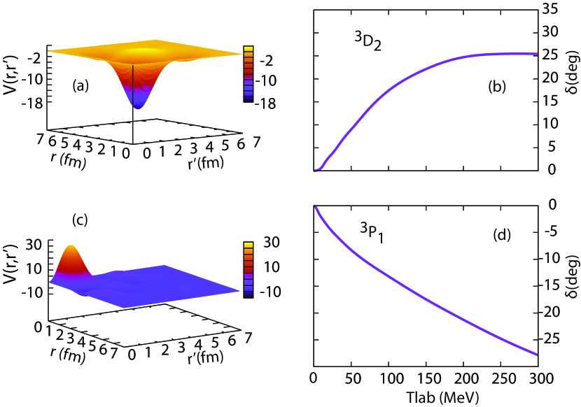
Figure 7: (Color online) Panels (a) and (c) : Non-local potentials produced using (17) for the JISP16 interaction and then utilized within CSM to calculate scattering phase shifts as depicted in Panels (b) and (d).

It is useful at this point to make an investigation on the precision of the results when varying the rotation angle $\theta$, discuss some current limitations and propose solutions for future applications. First of all we would like to mention that the CSM with Gaussian potentials cannot be applied for rotation angles larger than $\sim$ 0.78 radians ($\pi/4$) since the potential starts to appear singularities for larger values, so it would be useful to check the range of applicability when the interaction is realistic. We also refer the reader to an earlier work Rittby et al. (1981); *rittby2 where cases for rotation angles larger than the critical value of $\theta$ = $\pi/4$ where investigated.

It has been observed that when it comes to the phase-shifts (see also Papadimitriou and Vary (2015a)), there is indeed a rapid convergence of the results to the exact phase shift and the results are stable. We have noticed that the stability is numerically related to the distribution of the non-resonant scattering states along the $2\theta$ ray in the complex energy plane. If the distribution of the non-resonant solutions is to a good approximation close to the $2\theta$ ray, as it is also predicted by the ABC theorem, and the states do not depart much, then the phase shift calculated with (14) is equivalent to the exact one. On the contrary if the non-resonant continua are scattered, then the quality of the phase shift deteriorates. We show this behavior in Fig.8 where part of the solutions for the ³D₂ channel are shown and the corresponding phase shifts are calculated from this spectrum.

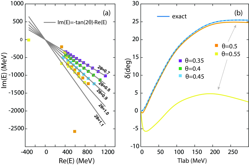
Figure 8: (Color online) Panel (a) : Part of the total ³D₂ eigenspectrum; it shows ten eigenvalues as a function of $\theta$ and as compared to the $2\theta$ ray which the ABC theorem predicts. Panel (b) : The corresponding phase shifts which were computed by using the solutions in (a) are shown.

Indeed, for rotation angles up to $\theta$=0.45 radians the calculated CSM phase shift is coinciding with the exact phase shift obtained by directly integrating the Shrödinger equation. Up to this point the complex eigenstates of the Hamiltonian (non-resonant continua) all fall almost exactly on a $2\theta$ path. For $\theta$ = 0.5 radians (orange points) the distribution of eigenstates is departing from the 2$\theta$ path and so the phase shift becomes less accurate, departing from the exact one. Of course for $\theta$ = 0.55 radians (yellow points) the eigenstates are even more scattered and the phase shift is much different from the exact one. Even though for practical applications a rotation angle of $\theta$ $\sim$ 0.4 radians is sufficient for revealing quite broad resonant states and also for convergence of observables, the stability issue for large rotation angles remains. This is something that is well known within the CSM calculations that also have employed a HO basis and in our case is also related to the fact that in order to create complex scaled matrix elements of the NN interaction we shift the transformation to the HO basis, which as it was already mentioned causes a large oscillatory behavior of the basis. It will be the topic of another publication to explore more flexible basis but still in the framework of employing realistic NN potentials and also try to tackle more precisely the numerical integration of functions that have large oscillatory behavior. It is also interesting to explore the possibility of generating pseudo-eigenstates that lie on a $2\theta$ trajectory and calculate phase shifts in this way. For phase shifts in particular it is sufficient to only know the complex eigenstates for each channel without the need to calculate eigenvectors. Knowing already the trajectory of these solutions on the complex energy plane it would be worth trying to generate artificial non resonant eigenstates, as if they were produced by the eigensolver, and use the CLD formula to compute the phase shift.

III.3 Backrotation application on deuteron for the dipole ³S₁-³D₁ $\to$ ³P₁ transition with a realistic force.

We move forward to test the Tikhonov backrotation on the calculation the dipole transition from the deuteron g.s. to the ³P₁ continuum channel (see also test studies in a different context using the LIT Leidemann (2015)). At this point our goal is not to benchmark the CSM method for calculating transitions with another method or compare with experiment, but we aim on testing the use of Tikhonov backrotated states for its calculation. Hence, for simplicity we have limited our selves to study the partial transition only to the ³P₁ channel. Of course the Tikhonov method is a regularization technique that regularizes the backrotation transformation and there should be no dependence of the regularization on whether the CSM solution comes from a toy model or a realistic Hamiltonian.

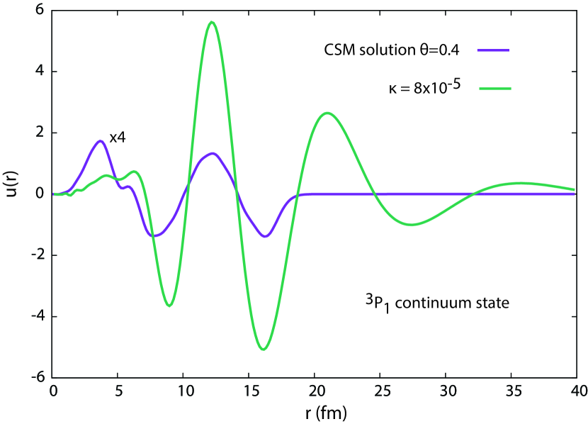
Figure 9: (Color online) Same as Fig.3 but for the ³P₁ non-resonant continuum wavefunction calculated with the JISP16 interaction. What is shown is the real part of the radial behavior of the fourth normalized non-resonant continuum ³P₁ solution that lies on the complex energy plane along a 2$\theta$ ray and $\theta$=0.4 radians. Also shown is the reconstructed backrotated Gamow solution. For better visualization the CSM solution was multiplied by a factor of 4.

We diagonalized the complex symmetric Hamiltonian matrix using a HO basis spanned by N=30 states and the CSM rotation angle was $\theta$ = 0.4 radians. In Fig.9 we present the CSM solution for the ³P₁ continuum channel, which in this case was the fourth continuum eigenstate. What is also shown is the reconstruction of the Gamow backrotated wavefunction using the Tikhonov technique for a regularization parameter $\kappa$ = 8$\times$10^-5. Then in Fig.10 we show the transition from the ³S₁-³D₁ g.s. to the ³P₁ continua, namely in Eq.12 the initial state is the deuteron g.s. and there is a sum over the HO basis complex scaled ³P₁ discretized continua which we have backrotated. As in the case of the Gaussian potential, the response calculated using the CSM solutions and the complex scaled dipole operator served as a benchmark (see Eq.11). We indeed observe that one can safely use the backrotated continua to calculate the response function with a more complicated and realistic interaction and there also exists a plateau of Tikhonov parameters for which the result coincides with the benchmark CSM one. This is an indication that backrotated non-resonant continua form a complete set in this case and actually the situation is the same with the one discussed around Fig.4.

IV Conclusions and perspectives

In this work we have explored more aspects of the Tikhonov backrotation process for the calculation of observables in CSM. In CSM even though one can conveniently determine resonant parameter of states above thresholds, the resonant and non-resonant states are all expressed as linear combinations of L² integrable functions. Hence they exhibit an asymptotic behavior which is permitted within the CSM, but is not the characteristic outgoing asymptotic behavior of a resonant state. This is not affecting calculation of a large variety of expectation values of operators that can be easily complex rotated. However it would always be useful within CSM to retrieve the correct asymptotic behavior of the Gamow wavefunction in calculations of excited states that are above particle thresholds. The Tikhonov method has proven to be suitable for this purpose.

We found out that the regularized backrotated Gamow wavefunction does not diverge at large distances which results in no special treatment for calculation of radial integrals. Even though the Gamow character was not fully retrieved this did not affect expectation values of observables in backrotated resonant states. This was shown by calculating expectation values of operators such as radii and response functions using the unrotated operator and the reconstructed Gamow functions. The method was tested on a system of two particles interacting via a Gaussian potential and also in the deuteron for studying the transition to the ³P₁ scattering state. We also investigated the orthogonality properties of the Gamow backrotated states for several regularization parameters and found out that they are not orthogonal.

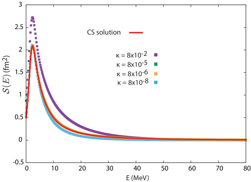
Figure 10: (Color online) Same as Fig.4 but for the transition from the deuteron g.s. to the ³P₁ continua and also using the realistic JISP16 interaction.

At the same time we explored some other features of the CSM, such as the ability to have access to both resonant parameters and also scattering quantities such as phase shifts. Within the schematic Gaussian model we were able to compare resonant parameters stemming from the CSM diagonalization and the scattering phase shift using the so-called inflection criterion. The inflection formula provided good results for resonances as broad as 600 keV whereas for broader resonances a complex energy method such as the CSM appears to be more accurate.

We studied the behavior of the CSM scattering eigenvalues for large rotation angles. For $\theta$ as large as 0.4 radians the scattering states are distributed along the, expected by the ABC theorem, 2$\theta$ line. We found out that this is the necessary condition to have stable and converged scattering phase shifts. Increasing the rotation angle to very large values causes the departure of the solutions from the 2$\theta$ line and at the same time the phase shift becomes unstable.

This problem would be treated by employing different L² basis sets for the discretization of the continuum which may increase precision of calculations and even use different complex energy eigenvalue solvers. In particular it is of interest to us to invest time on implementing L² basis for the discretization of the continuum in CSM that are defined on a grid such as Lagrange basis Baye (2015) or wavelet basis Cerioni et al. (2013), since it was recently shown that they can increase the precision, in particular the distribution of continuum states along the 2$\theta$ cuts of the complex energy plane. We would also like to use more advanced quadratures to integrate matrix elements between backrotated HO states or alternatively to regularize via the Tikhonov method the HO wavefunctions entering (18) and then use these states to express the complex scaled interaction matrix elements and check if results would stabilize for angles larger than $\theta$ $\sim$ 0.5 radians.