Guaranteed inference in topic models

Abstract

One of the core problems in statistical models is the estimation of a posterior distribution. For topic models, the problem of posterior inference for individual texts is particularly important, especially when dealing with data streams, but is often intractable in the worst case (Sontag and Roy, 2011). As a consequence, existing methods for posterior inference are approximate and do not have any guarantee on neither quality nor convergence rate. In this paper, we introduce a provably fast algorithm, namely Online Maximum a Posteriori Estimation (OPE), for posterior inference in topic models. OPE has more attractive properties than existing inference approaches, including theoretical guarantees on quality and fast rate of convergence to a local maximal/stationary point of the inference problem. The discussions about OPE are very general and hence can be easily employed in a wide range of contexts. Finally, we employ OPE to design three methods for learning Latent Dirichlet Allocation from text streams or large corpora. Extensive experiments demonstrate some superior behaviors of OPE and of our new learning methods.

Keywords: Topic models, posterior inference, online MAP estimation, theoretical guarantee, stochastic methods, non-convex optimization

1 Introduction

Latent Dirichlet allocation (LDA) (Blei et al., 2003) is the class of Bayesian networks that has gained arguably significant interests. It has found successful applications in a wide range of areas including text modeling (Blei, 2012), bioinformatics (Pritchard et al., 2000; Liu et al., 2010), history (Mimno, 2012), politics (Grimmer, 2010; Gerrish and Blei, 2012), psychology (Schwartz et al., 2013), to name a few.

One of the core issues in LDA is the estimation of posterior distributions for individual documents. The research community has been studying many approaches for this estimation problem, such as variational Bayes (VB) (Blei et al., 2003), collapsed variational Bayes (CVB) (Teh et al., 2007), CVB0 (Asuncion et al., 2009), and collapsed Gibbs sampling (CGS) (Griffiths and Steyvers, 2004; Mimno et al., 2012). Those approaches enable us to easily work with millions of texts (Mimno et al., 2012; Hoffman et al., 2013; Foulds et al., 2013). The quality of LDA in practice is determined by the quality of the inference method being employed. However, none of the mentioned methods has a theoretical guarantee on quality or convergence rate. This is a major drawback of existing inference methods.

Our first contribution in this paper is the introduction of a provably efficient algorithm, namely Online Maximum a Posteriori Estimation (OPE), for doing posterior inference of topic mixtures in LDA. This inference problem is in fact nonconvex and is NP-hard (Sontag and Roy, 2011; Arora et al., 2016). Our new algorithm is stochastic in nature and theoretically converges to a local maximal/stationary point of the inference problem. We prove that OPE converges at a rate of $O({1/T})$, which surpasses the best rate of existing stochastic algorithms for nonconvex problems (Mairal, 2013; Ghadimi and Lan, 2013), where $T$ is the number of iterations. Hence, OPE overcomes many drawbacks of VB, CVB, CVB0, and CGS. Those properties help OPE to be preferable in many contexts, and to provide us real benefits when using OPE in a wide class of probabilistic models.

The topic modeling literature has seen a fast growing interest in designing large-scale learning algorithms (Mimno et al., 2012; Than and Ho, 2012; Broderick et al., 2013; Foulds et al., 2013; Patterson and Teh, 2013; Hoffman et al., 2013; Than and Doan, 2014; Sato and Nakagawa, 2015). Existing algorithms allow us to easily analyze millions of documents. Those developments are of great significance, even though the posterior estimation is often intractable. Note that the performance of a learning method heavily depends on its core inference subroutine. Therefore, existing large-scale learning methods seem to likely remain some of the drawbacks from VB, CVB, CVB0, and CGS.

Our second contribution in this paper is the introduction of 3 stochastic algorithms for learning LDA at a large scale: Online-OPE which is online learning; Streaming-OPE which is streaming learning; and ML-OPE which is regularized online learning. These algorithms own the stochastic nature when learning global variables (topics), and employ OPE as the core for inferring local variables for individual texts, which is also stochastic. They overcome many drawbacks of existing large-scale learning methods owing to the preferable properties of OPE. From extensive experiments we find that Online-OPE, Streaming-OPE, and ML-OPE often reach very fast to a high predictiveness level, and are able to consistently increase the predictiveness of the learned models as observing more data. In paricular, while Online-OPE surpasses the state-of-the-art methods, ML-OPE often learns tens to thousand times faster than existing methods to reach the same predictiveness level. Therefore, our new methods are efficient tools for analyzing text streams or big collections.

Organization: in the next section we briefly discuss related work. In Section 3, we present the OPE algorithm for doing posterior inference. We also analyze the convergence property. We further compare OPE with existing inference methods, and discuss how to employ it in other contexts. Section 4 presents three stochastic algorithms for learning LDA from text streams or big text collections. Practical behaviors of large-scale learning algorithms and OPE will be investigated in Section 5. The final section presents some conclusions and discussions.

Notation: Throughout the paper, we use the following conventions and notations. Bold faces denote vectors or matrices. $x_{i}$ denotes the $i^{th}$ element of vector $\boldsymbol{x}$, and $A_{ij}$ denotes the element at row $i$ and column $j$ of matrix $\boldsymbol{A}$. The unit simplex in the $n$-dimensional Euclidean space is denoted as $\Delta_{n}=\{\boldsymbol{x}\in\mathbb{R}^{n}:\boldsymbol{x}\geq 0,\sum_{k=1}^{n}x_{k}=1\}$, and its interior is denoted as $\overline{\Delta}_{n}$. We will work with text collections with $V$ dimensions (dictionary size). Each document $\boldsymbol{d}$ will be represented as a frequency vector, $\boldsymbol{d}=(d_{1},...,d_{V})^{T}$ where $d_{j}$ represents the frequency of term $j$ in $\boldsymbol{d}$. Denote $n_{d}$ as the length of $\boldsymbol{d}$, i.e., $n_{d}=\sum_{j}d_{j}$. The inner product of vectors $\boldsymbol{u}$ and $\boldsymbol{v}$ is denoted as $\left<\boldsymbol{u},\boldsymbol{v}\right>$.

2 Related work

Notable inference methods for probabilistic topic models include VB, CVB, CVB0, and CGS. Except VB (Blei et al., 2003), most other methods originally have been developed for learning topic models from data. Fortunately, one can adapt them to do posterior inference for individual documents (Than and Ho, 2015). Other good candidates for doing posterior inference include Concave-Convex procedure (CCCP) by Yuille and Rangarajan (2003), Stochastic Majorization-Minimization (SMM) by Mairal (2013), Frank-Wolfe (FW) (Clarkson, 2010), Online Frank-Wolfe (OFW) (Hazan and Kale, 2012), and Thresholded Linear Inverse (TLI) which has been newly developed by Arora et al. (2016).

Few methods have an explicit theoretical guarantee on inference quality and convergence rate. In spite of being popularly used in topic modeling, we have not seen any theoretical analysis about how fast VB, CVB, CVB0, and CGS do inference for individual documents. One might employ CCCP (Yuille and Rangarajan, 2003) and SMM (Mairal, 2013) to do inference in topic models. Those two algorithms are guaranteed to converge to a stationary point of the inference problem. However, the convergence rate of CCCP and SMM is unknown for non-convex problems which are inherent in LDA and many other models. Each iteration of CCCP has to solve a (non-linear) equation system, which is expensive and non-trivial in many cases. Furthermore, up to now those two methods have not been investigated rigorously in the topic modeling literature.

It is worth discussing about FW (Than and Ho, 2015), OFW (Hazan and Kale, 2012), and TLI (Arora et al., 2016), the three methods with theoretical guarantees on quality. FW is a general method for convex programming (Clarkson, 2010). Than and Ho (2015, 2012) find that it can be effectively used to do inference for topic models. OFW is an online version of FW for convex problems whose objective functions come partly in an online fashion. One important property of FW and OFW is that they can converge fast and return sparse solutions. Nonetheless, FW and OFW only work with convex problems, and thus require some special settings/modifications for topic models. On the other hand, TLI has been proposed recently to do exact inference for individual texts. This is the only inference method which is able to recover solutions exactly under some assumptions. TLI requires that a document should be very long, and the topic matrix should have a small condition number. Those conditions might not always be present in practice. Therefore TLI is quite limited and should be improved further.

Two other algorithms for MAP estimation with provable guarantees are Particle Mirror Decent (PMD) (Dai et al., 2016) and HAMCMC (Simsekli et al., 2016). Both algorithms base on sampling to estimate a posterior distribution. Therefore they can be used to do posterior inference for topic models. PMC is shown to converge at a rate of $\mathcal{O}(T^{-1/2})$, while HAMCMC converges at a rate of $\mathcal{O}({T}^{-1/3})$ as suggested by Teh et al. (2016). Those are significant developments for Bayesian inference. However, their effectiveness in topic modeling is unclear at the time of writing this article.

In this work, we propose OPE for doing posterior inference. Unlike CCCP and SMM, OPE is guaranteed to converge very fast to a local maximal/stationary point of the inference problem. The convergence rate of OPE is faster than that of PMD and HAMCMC. Each iteration of OPE requires modest arithmetic operations and thus OPE is significantly more efficient than CCCP, SMM, PMD, and HAMCMC. Having an explicit guarantee helps OPE to overcome many limitations of VB, CVB, CVB0, and CGS. Further, OPE is so general that it can be easily employed in a wide range of contexts, including MAP estimation and non-convex optimization. Therefore, OPE overcomes some drawbacks of FW, OFW, and TLI. Table 1 presents more details to compare OPE and various inference methods.

3 Posterior inference with OPE

LDA (Blei et al., 2003) is a generative model for modeling texts and discrete data. It assumes that a corpus is composed from $K$ topics $\boldsymbol{\beta}_{1},...,\boldsymbol{\beta}_{K}$, each of which is a sample from a $V$-dimensional Dirichlet distribution, $Dirichlet(\eta)$. A document $\boldsymbol{d}$ arises from the following generative process:

1. Draw $\boldsymbol{\theta}_{d}|\alpha\sim Dirichlet(\alpha)$

2. For the $n^{th}$ word of $\boldsymbol{d}$:

   • draw topic index $z_{dn}|\boldsymbol{\theta}_{d}\sim Multinomial(\boldsymbol{\theta}_{d})$

   • draw word $w_{dn}|z_{dn},\boldsymbol{\beta}\sim Multinomial(\boldsymbol{\beta}_{z_{dn}})$.

Each topic mixture $\boldsymbol{\theta}_{d}=(\theta_{d1},...,\theta_{dK})$ represents the contributions of topics to document $\boldsymbol{d}$, while $\beta_{kj}$ shows the contribution of term $j$ to topic $k$. Note that $\boldsymbol{\theta}_{d}\in\Delta_{K},\boldsymbol{\beta}_{k}\in\Delta_{V},\forall k$. Both $\boldsymbol{\theta}_{d}$ and $\boldsymbol{z}_{d}$ are unobserved variables and are local for each document.

According to Teh et al. (2007), the task of Bayesian inference (learning) given a corpus $\mathcal{C}=\{\boldsymbol{d}_{1},...,\boldsymbol{d}_{M}\}$ is to estimate the posterior distribution $p(\boldsymbol{z,\theta,\beta}|\mathcal{C},\alpha,\eta)$ over the latent topic indicies $\boldsymbol{z}=\{\boldsymbol{z}_{1},...,\boldsymbol{z}_{d}\}$, topic mixtures $\boldsymbol{\theta}=\{\boldsymbol{\theta}_{1},...,\boldsymbol{\theta}_{M}\}$, and topics $\boldsymbol{\beta}=(\boldsymbol{\beta}_{1},...,\boldsymbol{\beta}_{K})$. The problem of posterior inference for each document $\boldsymbol{d}$, given a model $\{\boldsymbol{\beta},\alpha\}$, is to estimate the full joint distribution $p(\boldsymbol{z}_{d},\boldsymbol{\theta}_{d},\boldsymbol{d}|\boldsymbol{\beta},\alpha)$. Direct estimation of this distribution is intractable. Hence existing approaches uses different schemes. VB, CVB, and CVB0 try to estimate the distribution by maximizing a lower bound of the likelihood $p(\boldsymbol{d}|\boldsymbol{\beta},\alpha)$, whereas CGS (Mimno et al., 2012) tries to estimate $p(\boldsymbol{z}_{d}|\boldsymbol{d},\boldsymbol{\beta},\alpha)$. For a detailed discussion and comparison of those methods, the reader should refer to Than and Ho (2015).

3.1 MAP inference of topic mixtures

We now consider the MAP estimation of topic mixture for a given document $\boldsymbol{d}$:

$$\boldsymbol{\theta}^{*}=\arg\max_{\boldsymbol{\theta}\in\Delta_{K}}\Pr(\boldsymbol{\theta},\boldsymbol{d}|\boldsymbol{\beta},\alpha)=\arg\max_{\boldsymbol{\theta}\in\Delta_{K}}\Pr(\boldsymbol{d}|\boldsymbol{\theta},\boldsymbol{\beta})\Pr(\boldsymbol{\theta}|\alpha).$$ (1)

Than and Ho (2015) show that this problem is equivalent to the following one:

$$\boldsymbol{\theta}^{*}=\arg\max_{\boldsymbol{\theta}\in\Delta_{K}}\sum_{j}d_{j}\log\sum_{k=1}^{K}\theta_{k}\beta_{kj}+(\alpha-1)\sum_{k=1}^{K}\log\theta_{k}.$$ (2)

Sontag and Roy (2011) showed that this problem is NP-hard in the worst case when $\alpha<1$. In the case of $\alpha\geq 1$, one can easily show that the problem (2) is concave, and therefore it can be solved in polynomial time. Unfortunately, in practice of LDA, the parameter $\alpha$ is often small, says $\alpha<1$, causing (2) to be nonconcave. That is the reason for why (2) is intractable in the worst case.

We present a novel algorithm (OPE) for doing inference of topic mixtures for documents. The idea of OPE is quite simple. It solves problem (2) by iteratively finding a good vertex of $\overline{\Delta}_{K}=\{\boldsymbol{x}\in\mathbb{R}^{K}:\sum_{k=1}^{K}x_{k}=1,\boldsymbol{x}\geq\epsilon>0\}$ to improve its solution. A good vertex at each iteration is decided by assessing stochastic approximations to the gradient of the objective function $f(\boldsymbol{\theta})$. When the number of iterations goes to infinity, OPE will approach to a local maximal/stationary point of problem (2). Details of OPE is presented in Algorithm 1.

Algorithm 1 OPE: Online maximum a posteriori estimation

  Input: document $\boldsymbol{d}$, and model $\{\boldsymbol{\beta},\alpha\}$.

  Output: $\boldsymbol{\theta}$ that maximizes $f(\boldsymbol{\theta})=\sum_{j}d_{j}\log\sum_{k=1}^{K}\theta_{k}\beta_{kj}+(\alpha-1)\sum_{k=1}^{K}\log\theta_{k}.$

  Initialize $\boldsymbol{\theta}_{1}$ arbitrarily in $\overline{\Delta}_{K}=\{\boldsymbol{x}\in\mathbb{R}^{K}:\sum_{k=1}^{K}x_{k}=1,\boldsymbol{x}\geq\epsilon>0\}$.

  for  $t=1,...,\infty$ do

     Pick $f_{t}$ uniformly from $\;\;\;\{\sum_{j}d_{j}\log\sum_{k=1}^{K}\theta_{k}\beta_{kj};\;\;(\alpha-1)\sum_{k=1}^{K}\log\theta_{k}\}$

     $F_{t}:=\frac{2}{t}\sum_{h=1}^{t}f_{h}$

     $\boldsymbol{e}_{t}:=\arg\max_{\boldsymbol{x}\in\overline{\Delta}_{K}}\left<F^{\prime}_{t}(\boldsymbol{\theta}_{t}),\boldsymbol{x}\right>\;\;\;\;$ (the vertex of $\overline{\Delta}_{K}$ that follows the maximal gradient)

     $\boldsymbol{\theta}_{t+1}:=\boldsymbol{\theta}_{t}+(\boldsymbol{e}_{t}-\boldsymbol{\theta}_{t})/t$

  end for

3.2 Convergence analysis

In this section, we prove the convergence of OPE which appears in Theorem 2. We need the following observations.

Lemma 1

Let $\{X_{1},X_{2},...\}$ be a sequence of uniformly i.i.d. random variables on $\{-1,1\}$. (Each $X_{i}$ is also known as a Rademacher random variable.) The followings hold for the sequence $S_{n}=X_{1}+X_{2}+\cdots+X_{n}$:

1. $\frac{S_{n}}{n}\rightarrow 0$ as $n\rightarrow+\infty$.

2. There exist constants $v\in[0,1)$ and $N_{0}>1$ such that $\forall n\geq N_{0},|S_{n}|\leq n^{v}$ (equivalently, $\log_{n}|S_{n}|\leq v$).

Proof  Let $a_{n}$ (and $b_{n}$ respectively) be the number of times that $1$ (and $-1$) appears in the sum $X_{1}+X_{2}+\cdots+X_{n}$. So $a_{n}+b_{n}=n$ and $S_{n}=a_{n}-b_{n}$. If $S_{n}=cn$ for some $c$, then $a_{n}=(c+1)n/2,b_{n}=(1-c)n/2$. Since $X_{i}$ is picked uniformly from $\{-1,1\}$ for every $i$, both $a_{n}/n$ and $b_{n}/n$ go to 0.5 as $n\rightarrow+\infty$. This suggests that $c$ goes to 0 as $n\rightarrow+\infty$. Therefore $\frac{S_{n}}{n}\rightarrow 0$ as $n\rightarrow+\infty$.

We will prove the second result by contrapositive. Assume

$$\forall v\in[0,1),\forall N_{0}>1,\exists n\geq N_{0}\text{ such that }\log_{n}|S_{n}|>v.$$ (3)

Take an infinite sequence $v_{t}\in[0,1)$ such that $v_{t}\rightarrow 1$ as $t\rightarrow+\infty$. Then statement (3) implies that $\forall t\geq 1,\exists n_{t}$ satisfying

$$\log_{n_{1}}(n_{1}+1) > \log_{n_{1}}|S_{n_{1}}|>v_{1},$$

$$\log_{n_{t}}(n_{t}+1) > \log_{n_{t}}|S_{n_{t}}|>v_{t},$$ (4)

$$n_{t} > n_{t-1}\text{ for }t\geq 2.$$

It is easy to see that $\log_{n_{t}}(n_{t}+1)\rightarrow 1$ as $t\rightarrow\infty$. Therefore $\log_{n_{t}}|S_{n_{t}}|\rightarrow 1$ as $t\rightarrow\infty$. In other words, $|S_{n_{t}}|\rightarrow n_{t}$ as $t\rightarrow\infty$. This is in contrary to the first result. Hence the second result holds.  

Theorem 2 (Convergence)

Consider the objective function $f(\boldsymbol{\theta})$ in problem (2), given fixed $\boldsymbol{d},\boldsymbol{\beta},\alpha$. For Algorithm 1, the followings hold

1. For any $\boldsymbol{\theta}\in\overline{\Delta}_{K}$, $F_{t}\left(\boldsymbol{\theta}\right)$ converges to $f\left(\boldsymbol{\theta}\right)$ as ${t}\rightarrow+\infty$,

2. $\boldsymbol{\theta}_{t}$ converges to a local maximal/stationary point $\boldsymbol{\theta}^{*}$ of $f$ at a rate of $\mathcal{O}(1/t)$.

Proof  Denote $g_{1}=\sum_{j}d_{j}\log\sum_{k=1}^{K}\theta_{k}\beta_{kj}$ and $g_{2}=(\alpha-1)\sum_{k=1}^{K}\log\theta_{k}$, we have $f=g_{1}+g_{2}$. Let $a_{t}$ and $b_{t}$ be the number of times that we have already picked $g_{1}$ and $g_{2}$ respectively after $t$ iterations. Note that $a_{t}+b_{t}=t$. Therefore for any $\boldsymbol{\theta}\in\overline{\Delta}_{K}$ we have

$$F_{t} = \frac{2}{t}(a_{t}g_{1}+b_{t}g_{2})$$ (5)

$$F_{t}-f = \frac{a_{t}-b_{t}}{t}(g_{1}-g_{2})=\frac{S_{t}}{t}(g_{1}-g_{2})$$ (6)

$$F^{\prime}_{t}-f^{\prime} = \frac{a_{t}-b_{t}}{t}(g^{\prime}_{1}-g^{\prime}_{2})=\frac{S_{t}}{t}(g^{\prime}_{1}-g^{\prime}_{2}),$$ (7)

where we have denoted $S_{t}=a_{t}-b_{t}$.

For each iteration $t$ of OPE we have to pick uniformly randomly an $f_{t}$ from $\{g_{1},g_{2}\}$. Now we make a correspondence between $f_{t}$ and a uniformly random variable $X_{t}$ on $\{1,-1\}$. This correspondence is a one-to-one mapping. So $S_{t}$ can be represented as $S_{t}=X_{1}+\cdots+X_{t}$. Lemma 1 shows that $S_{t}/t\rightarrow 0$ as $t\rightarrow\infty$. Combining this with (6) we conclude that the sequence ${F_{t}}$ converges to $f$. Also due to (7), the sequence $F^{\prime}_{t}$ converges to $f^{\prime}$. The convergence holds for any $\boldsymbol{\theta}\in\overline{\Delta}_{K}$. This proves the first statement of the theorem.

It is easy to see that the sequence $\{\boldsymbol{\theta}_{1},\boldsymbol{\theta}_{2},...\}$ converges to a point $\boldsymbol{\theta}^{*}\in\overline{\Delta}_{K}$ at the rate $\mathcal{O}(1/t)$, due to the update of $\boldsymbol{\theta}_{t+1}:=\boldsymbol{\theta}_{t}+(\boldsymbol{e}_{t}-\boldsymbol{\theta}_{t})/t$. We next show that $\boldsymbol{\theta}^{*}$ is a local maximal/stationary point of $f$.

Consider

$$\left\langle F^{\prime}_{t}(\boldsymbol{\theta}_{t}),\frac{\boldsymbol{e}_{t}-\boldsymbol{\theta}_{t}}{t}\right\rangle = \left\langle F^{\prime}_{t}(\boldsymbol{\theta}_{t})-f^{\prime}(\boldsymbol{\theta}_{t}),\frac{\boldsymbol{e}_{t}-\boldsymbol{\theta}_{t}}{t}\right\rangle+\left\langle f^{\prime}(\boldsymbol{\theta}_{t}),\frac{\boldsymbol{e}_{t}-\boldsymbol{\theta}_{t}}{t}\right\rangle$$ (8)

$$= \left\langle\frac{S_{t}}{t}(g^{\prime}_{1}(\boldsymbol{\theta}_{t})-g^{\prime}_{2}(\boldsymbol{\theta}_{t})),\frac{\boldsymbol{e}_{t}-\boldsymbol{\theta}_{t}}{t}\right\rangle+\left\langle f^{\prime}(\boldsymbol{\theta}_{t}),\frac{\boldsymbol{e}_{t}-\boldsymbol{\theta}_{t}}{t}\right\rangle$$ (9)

$$= \frac{S_{t}}{t^{2}}\left\langle g^{\prime}_{1}(\boldsymbol{\theta}_{t})-g^{\prime}_{2}(\boldsymbol{\theta}_{t}),{\boldsymbol{e}_{t}-\boldsymbol{\theta}_{t}}\right\rangle+\left\langle f^{\prime}(\boldsymbol{\theta}_{t}),\frac{\boldsymbol{e}_{t}-\boldsymbol{\theta}_{t}}{t}\right\rangle$$ (10)

Note that $g_{1},g_{2}$ are Lipschitz continuous on $\overline{\Delta}_{K}$. Hence there exists a constant $L$ such that

$$\left<f^{\prime}(z),y-z\right> \leq f(y)-f(z)+L||y-z||^{2},\forall z,y\in\overline{\Delta}_{K}$$ (11)

Exploiting this to (10) we obtain

$$\left\langle F^{\prime}_{t}(\boldsymbol{\theta}_{t}),\frac{\boldsymbol{e}_{t}-\boldsymbol{\theta}_{t}}{t}\right\rangle \leq \frac{S_{t}}{t^{2}}\left\langle g^{\prime}_{1}(\boldsymbol{\theta}_{t})-g^{\prime}_{2}(\boldsymbol{\theta}_{t}),{\boldsymbol{e}_{t}-\boldsymbol{\theta}_{t}}\right\rangle+f(\boldsymbol{\theta}_{t+1})-f(\boldsymbol{\theta}_{t})+\frac{L}{t^{2}}||\boldsymbol{e}_{t}-\boldsymbol{\theta}_{t}||^{2}.$$

Since $\boldsymbol{e}_{t}$ and $\boldsymbol{\theta}_{t}$ belong to $\Delta_{K}$, the quantity $|\left\langle g^{\prime}_{1}(\boldsymbol{\theta}_{t})-g^{\prime}_{2}(\boldsymbol{\theta}_{t}),{\boldsymbol{e}_{t}-\boldsymbol{\theta}_{t}}\right\rangle|$ is bounded above for any $t$. Therefore, there exists a constant $c_{2}>0$ such that

$$\left\langle F^{\prime}_{t}(\boldsymbol{\theta}_{t}),\frac{\boldsymbol{e}_{t}-\boldsymbol{\theta}_{t}}{t}\right\rangle \leq \frac{c_{2}|S_{t}|}{t^{2}}+f(\boldsymbol{\theta}_{t+1})-f(\boldsymbol{\theta}_{t})+\frac{c_{2}L}{t^{2}}.$$ (12)

Summing both sides of (12) for all $t$ we have

$$\sum_{h=1}^{t}\frac{1}{h}\left\langle F^{\prime}_{h}(\boldsymbol{\theta}_{h}),\boldsymbol{e}_{h}-\boldsymbol{\theta}_{h}\right\rangle \leq \sum_{h=1}^{t}\frac{c_{2}|S_{h}|}{h^{2}}+f(\boldsymbol{\theta}_{t+1})-f(\boldsymbol{\theta}_{1})+\sum_{h=1}^{t}\frac{c_{2}L}{h^{2}}.$$ (13)

As $t\rightarrow+\infty$ we note that $f(\boldsymbol{\theta}_{t})\rightarrow f(\boldsymbol{\theta}^{*})$ due to the continuity of $f$. As a result, inequality (13) implies

$$\sum_{h=1}^{+\infty}\frac{1}{h}\left\langle F^{\prime}_{h}(\boldsymbol{\theta}_{h}),\boldsymbol{e}_{h}-\boldsymbol{\theta}_{h}\right\rangle \leq \sum_{h=1}^{+\infty}\frac{c_{2}|S_{h}|}{h^{2}}+f(\boldsymbol{\theta}^{*})-f(\boldsymbol{\theta}_{1})+\sum_{h=1}^{+\infty}\frac{c_{2}L}{h^{2}}.$$ (14)

According to Lemma 1, there exist constants $v\in[0,1)$ and $T_{0}>1$ such that $\forall t\geq T_{0},|S_{t}|\leq t^{v}$. Therefore

$$\sum_{h=1}^{+\infty}\frac{1}{h}\left\langle F^{\prime}_{h}(\boldsymbol{\theta}_{h}),\boldsymbol{e}_{h}-\boldsymbol{\theta}_{h}\right\rangle \leq c_{2}\sum_{h=1}^{T_{0}}\frac{|S_{h}|}{h^{2}}+c_{2}\sum_{h=T_{0}+1}^{+\infty}\frac{h^{v}}{h^{2}}+f(\boldsymbol{\theta}^{*})-f(\boldsymbol{\theta}_{1})+\sum_{h=1}^{+\infty}\frac{c_{2}L}{h^{2}}.$$ (15)

Note that the series $\sum_{h=T_{0}+1}^{+\infty}{h^{v}/h^{2}}$ converges due to $v\in[0,1)$, and $\sum_{h=1}^{T_{0}}{|S_{h}|}/{h^{2}}$ is bounded. Further, $\sum_{h=1}^{+\infty}{L}/{h^{2}}<\infty$. Hence, the right-hand side of (15) is finite. In addition, $\left\langle F^{\prime}_{h}(\boldsymbol{\theta}_{h}),\boldsymbol{e}_{h}\right\rangle>\left\langle F^{\prime}_{h}(\boldsymbol{\theta}_{h}),\boldsymbol{\theta}_{h}\right\rangle$ for any $h>0$ because of $\boldsymbol{e}_{h}=\arg\max_{\boldsymbol{x}\in\overline{\Delta}_{K}}\left\langle F^{\prime}_{h}(\boldsymbol{\theta}_{h}),\boldsymbol{x}\right\rangle$. Therefore we obtain the following

$$0\leq\sum_{h=1}^{+\infty}\frac{1}{h}\left\langle F^{\prime}_{h}(\boldsymbol{\theta}_{h}),\boldsymbol{e}_{h}-\boldsymbol{\theta}_{h}\right\rangle < \infty.$$ (16)

In other words, the series $\sum_{h=1}^{+\infty}\frac{1}{h}\left\langle F^{\prime}_{h}(\boldsymbol{\theta}_{h}),\boldsymbol{e}_{h}-\boldsymbol{\theta}_{h}\right\rangle$ converges to a finite constant.

Note that $0\leq\left\langle F^{\prime}_{h}(\boldsymbol{\theta}_{h}),\boldsymbol{e}_{h}-\boldsymbol{\theta}_{h}\right\rangle$ for any $h$. If there exists constant $c_{3}>0$ satisfying $\left\langle F^{\prime}_{h}(\boldsymbol{\theta}_{h}),\boldsymbol{e}_{h}-\boldsymbol{\theta}_{h}\right\rangle\geq c_{3}$ for an infinite number of $h$’s, then the series $\sum_{h=1}^{+\infty}\frac{1}{h}\left\langle F^{\prime}_{h}(\boldsymbol{\theta}_{h}),\boldsymbol{e}_{h}-\boldsymbol{\theta}_{h}\right\rangle$ could not converge to a finite constant, which is in contrary to (16). Therefore,

$$\left\langle F^{\prime}_{h}(\boldsymbol{\theta}_{h}),\boldsymbol{e}_{h}-\boldsymbol{\theta}_{h}\right\rangle\rightarrow 0\text{ as }h\rightarrow+\infty.$$ (17)

In one case, there exists a large $H$ such that $|\boldsymbol{e}_{h}-\boldsymbol{\theta}_{h}|\rightarrow 0$ for any $h\geq H$. This suggests one of the vertex of $\overline{\Delta}_{K}$ is a local maximal point of $f$, which proves the theorem. On the other case, assume that the sequence $\boldsymbol{e}_{h}-\boldsymbol{\theta}_{h}$ diverges or converges to a nonzero constant $c_{4}$. Then (17) holds if and only if $F^{\prime}_{h}(\boldsymbol{\theta}_{h})$ goes to 0 as $h\rightarrow+\infty$. Since $\boldsymbol{\theta}_{h}\rightarrow\boldsymbol{\theta}^{*}$, we have

$$\lim\limits_{h\rightarrow+\infty}||F^{\prime}_{h}(\boldsymbol{\theta}_{h})||=\lim\limits_{h\rightarrow+\infty}||f^{\prime}(\boldsymbol{\theta}_{h})||=||f^{\prime}(\boldsymbol{\theta}^{*})||=0.$$ (18)

In other words, $\boldsymbol{\theta}^{*}$ is a stationary point of $f$.

 

3.3 Comparison with existing inference methods

Table 1: Theoretical comparison of 5 inference methods, given a document $\boldsymbol{d}$ and model $\mathcal{M}$ with $K$ topics. MAP denotes maximum a posterior, ELBO denotes maximizing an evidence lower bound on the likelihood. $T$ denotes the number of iterations. $n_{d}$ and $\ell_{d}$ respectively are the number of different terms and number of tokens in $\boldsymbol{d}$. ‘-’ denotes ‘unknown’. Note that $n_{d}\leq\ell_{d}$.

Method	OPE	VB	CVB	CVB0	CGS
Posterior probability of interest	$\Pr(\boldsymbol{\theta,d}|\mathcal{M})$	$\Pr(\boldsymbol{\theta,z,d}|\mathcal{M})$	$\Pr(\boldsymbol{z,d}|\mathcal{M})$	$\Pr(\boldsymbol{z,d}|\mathcal{M})$	$\Pr(\boldsymbol{z,d}|\mathcal{M})$
Approach	MAP	ELBO	ELBO	ELBO	Sampling
Quality bound	Yes	-	-	-	-
Convergence rate	$O(1/T)$	-	-	-	-
Iteration complexity	$O(K.n_{d})$	$O(K.n_{d})$	$O(K.\ell_{d})$	$O(K.\ell_{d})$	$O(K.\ell_{d})$
Storage	$O(K)$	$O(K.n_{d})$	$O(K.\ell_{d})$	$O(K.\ell_{d})$	$O(K.\ell_{d})$
$Digamma$ evaluations	0	$O(K.n_{d})$	0	0	$O(K.n_{d})$
$Exp$ or $Log$ evaluations	$O(K.n_{d})$	$O(K.n_{d})$	$O(K.\ell_{d})$	0	$O(K.n_{d})$
Modification on global variables	No	No	Yes	Yes	No

Comparing with other inference approaches (including VB, CVB, CVB0 and CGS), our algorithm has many preferable properties as summarized in Table 1.

• OPE has explicitly theoretical guarantees on quality and fast convergence rate. This is the most notable property of OPE, for which existing inference methods often do not have.

• Its rate of convergence surpasses the best rate of existing stochastic algorithms for non-convex problems (Ghadimi and Lan, 2013; Mairal, 2013). Note that OPE can be easily modified to solve more general non-convex problems. Therefore, it is applicable to a wide range of contexts.

• OPE requires a very modest memory of $O(K)$ for storing temporary solutions and gradients, which is significantly more efficient than VB, CVB, CVB0, and CGS.

• Each iteration of OPE requires $O(Kn_{d})$ computations for computing gradients and updating solutions. This is much more efficient than VB, CVB, CVB0, and CGS in practice.

• Unlike CVB and CVB0, OPE does not change the global variables when doing inference for individual documents. Hence OPE embarrasingly enables parallel inference, and is more beneficial than CVB and CVB0.

3.4 Extension to MAP estimation and non-convex optimization

It is worth realizing that the employment of OPE for other contexts is straightforward. The main step of using OPE is to formulate the problem of interest to be maximization of a function of the form $f(x)=g_{1}(x)+g_{2}(x)$. In the followings, we demonstrate this main step in two problems which appear in a wide range of contexts.

The MAP estimation problem in many probabilistic models is the task of finding an

$$x^{*}=\arg\max_{x}\Pr(x|D)=\arg\max_{x}\Pr(D|x)\Pr(x)/\Pr(D),$$

where $\Pr(D|x)$ denotes the likelihood of an observed variable $D$, $\Pr(x)$ denotes the prior of the hidden variable $x$, and $\Pr(D)$ denotes the marginal probability of $D$. Note that

$$x^{*}=\arg\max_{x}\Pr(D|x)\Pr(x)=\arg\max_{x}[\log\Pr(D|x)+\log\Pr(x)].$$

If the densities of the distributions over $x$ and $D$ can be described by some analytic functions, then the MAP estimation problem turns out to be maximization of $f(x)=g_{1}(x)+g_{2}(x)$, where $g_{1}(x)=\log\Pr(D|x),g_{2}(x)=\log\Pr(x)$.

Now consider a general non-convex optimization problem $x^{*}=\arg\max_{x}f(x)$. Theorem 1 by Yuille and Rangarajan (2003) shows that we can always decompose $f(x)$ into the sum of a convex function and a concave function, provided that $f(x)$ has bounded Hessian. This is one way to decompose $f$ into the sum of two functions. We can use many other ways to make a decomposition of $f=g_{1}+g_{2}$ and then employ OPE, because the convergence proof of OPE does not require $g_{1}$ and $g_{2}$ to be concave/convex.

The analysis above demonstrates that OPE can be easily employed in a wide range of contexts, including posterior estimation and non-convex optimization. One may need to suitably modify the domain of $\boldsymbol{\theta}$, and hence the step of finding $\boldsymbol{e}_{t}$ will be a linear program which can be solved efficiently. Comparing with non-linear steps in CCCP (Yuille and Rangarajan, 2003) and SMM (Mairal, 2013), OPE could be much more efficient. In this paper, we do not try to make a rigorous investigation of OPE in those contexts, and leave it open for future research.

4 Stochastic algorithms for learning LDA

We have seen many attractive properties of OPE that other methods do not have. We further show in this section the simplicity of using OPE for designing fast learning algorithms for topic models. More specifically, we design 3 algorithms: Online-OPE which learns LDA from large corpora in an online fashion, Streaming-OPE which learns LDA from data streams, and ML-OPE which enables us to learn LDA from either large corpora or data streams. These algorithms employ OPE to do MAP inference for individual documents, and the online scheme (Bottou, 1998; Hoffman et al., 2013) or streaming scheme (Broderick et al., 2013) to infer global variables (topics). Hence, the stochastic nature appears in both local and global inference phases. Note that the MAP inference of local variables by OPE has theoretical guarantees on quality and convergence rate. Such a property might help the new large-scale learning algorithms be more attractive than existing ones, which base on VB, CVB, CVB0, and CGS.

4.1 Regularized online learning

Given a corpus $\mathcal{C}$ (with finite or infinite number of documents) and $\alpha>0$, we will estimate the topics $\boldsymbol{\beta}_{1},...,\boldsymbol{\beta}_{K}$ that maximize

$$\begin{split}\mathcal{L}(\boldsymbol{\beta})&=\sum_{\boldsymbol{d}\in\mathcal{C}}\log\Pr\left(\boldsymbol{\theta}_{d},\boldsymbol{d}|\boldsymbol{\beta},\alpha\right)\\ &=\sum_{\boldsymbol{d}\in\mathcal{C}}\left(\sum_{j}d_{j}\log\sum_{k=1}^{K}\theta_{dk}\beta_{kj}+(\alpha-1)\sum_{k=1}^{K}\log\theta_{dk}\right)+constant.\end{split}$$ (19)

To solve this problem, we use the online learning scheme by Bottou (1998). More specifically, we repeat the following steps:

• Sample a subset $\mathcal{C}_{t}$ of documents from $\mathcal{C}$. Infer the local variables ($\boldsymbol{\theta}_{d}$) for each document $\boldsymbol{d}\in\mathcal{C}_{t}$, given the global variable $\boldsymbol{\beta}^{t-1}$ in the last step.

• Form an intermediate global variable $\hat{\boldsymbol{\beta}}^{t}$ for $\mathcal{C}_{t}$.

• Update the global variable to be a weighted average of $\hat{\boldsymbol{\beta}}^{t}$ and $\boldsymbol{\beta}^{t-1}$.

Details of this learning algorithm is presented in Algorithm 2, where we have used the same arguments as Than and Ho (2012) to update the intermediate topics $\hat{\boldsymbol{\beta}}^{t}$ from $\mathcal{C}_{t}$:

$$\hat{\beta}^{t}_{kj}\propto\sum_{\boldsymbol{d}\in\mathcal{C}_{t}}d_{j}\theta_{dk}.$$ (20)

Note that in Algorithm 2 the step-size $\rho_{t}=\left(t+\tau\right)^{-\kappa}$ satisfies two conditions: $\sum_{t=1}^{\infty}\rho_{t}=\infty$ and $\sum_{t=1}^{\infty}\rho_{t}^{2}<\infty$. These conditions are to assure that the learning algorithm will converge to a stationary point (Bottou, 1998). $\kappa\in(0.5,1]$ is the forgeting rate, the higher the lesser the algorithm weighs the role of new data.

Algorithm 2 ML-OPE for learning LDA from massive/streaming data

  Input: data sequence, $K,\alpha,\tau>0,\kappa\in(0.5,1]$

  Output: $\boldsymbol{\beta}$

  Initialize $\boldsymbol{\beta}^{0}$ randomly in $\Delta_{V}$

  for  $t=1,...,\infty$ do

     Pick a set $\mathcal{C}_{t}$ of documents

     Do inference by OPE for each $\boldsymbol{d}\in\mathcal{C}_{t}$ to get $\boldsymbol{\theta}_{d}$, given $\boldsymbol{\beta}^{t-1}$

     Compute intermediate topics $\hat{\boldsymbol{\beta}}^{t}$ as:

$$\hat{\beta}_{kj}^{t}\propto\sum_{\boldsymbol{d}\in\mathcal{C}_{t}}d_{j}\theta_{dk}$$ (21)

     Set step-size: $\rho_{t}=\left(t+\tau\right)^{-\kappa}$

     Update topics: $\boldsymbol{\beta}^{t}:=\left(1-\rho_{t}\right)\boldsymbol{\beta}^{t-1}+\rho_{t}\hat{\boldsymbol{\beta}}^{t}$

  end for

It is worth discussing some fundamental differences between ML-OPE and existing online/streaming methods. First, we need not to know a priori how many documents to be processed. Hence, ML-OPE can deal well with streaming/online environments in a realistical way. Second, ML-OPE learns topics ($\boldsymbol{\beta}$) directly instead of learning the parameter ($\boldsymbol{\lambda}$) of a variarional distribution over topics as in SVI (Hoffman et al., 2013), in SSU (Broderick et al., 2013), and in the hybrid method by Mimno et al. (2012). While $\boldsymbol{\beta}$ are regularized to be in the unit simplex $\Delta_{V}$, $\boldsymbol{\lambda}$ can grow arbitrarily. The uncontrolled growth of $\boldsymbol{\lambda}$ might potentially cause overfitting as sufficiently many documents are processed. In contrast, the regularization on $\boldsymbol{\beta}$ helps ML-OPE to avoid overfitting and generalize better.

4.2 Online and streaming learning

In the existing literature of topic modeling, most methods for posterior inference try to estimate $\Pr(\boldsymbol{\theta,z,d}|\mathcal{M})$ or $\Pr(\boldsymbol{z,d}|\mathcal{M})$ given a model $\mathcal{M}$ and document $\boldsymbol{d}$. Therefore, existing large-scale learning algorithms for topic models often base on those probabilities. Some examples include SVI (Hoffman et al., 2013), SSU (Broderick et al., 2013), SCVB0 (Foulds et al., 2013; Sato and Nakagawa, 2015), Hybrid sampling and SVI (Mimno et al., 2012), Population-VB (McInerney et al., 2015).

Different with other approaches, OPE directly infers $\boldsymbol{\theta}$ by maximizing the joint probability $\Pr(\boldsymbol{\theta,d}|\mathcal{M})$. Following the same arguments with Than and Ho (2015), one can easily exploit OPE to design new online and streaming algorithms for learning LDA. Online-OPE in Algorithm 3 and Streaming-OPE in Algorithm 4 are two exploitations of OPE. It is worth noting that Online-OPE and Streaming-OPE are hybrid combinations of OPE with SVI, which are similar in manner to the algorithm by Mimno et al. (2012). Further, Streaming-OPE and ML-OPE do not need to know a priori the number of documents to be processed in the future, and hence are suitable to work in a real streaming environment.

Algorithm 3 Online-OPE for learning LDA from massive data

  Input: training data $\mathcal{C}$ with $D$ documents, $K,\alpha,\eta,\tau>0,\kappa\in(0.5,1]$

  Output: $\boldsymbol{\lambda}$

  Initialize $\boldsymbol{\lambda}^{0}$ randomly

  for  $t=1,...,\infty$ do

     Sample a set $\mathcal{C}_{t}$ consisting of $S$ documents.

     Use Algorithm 1 to do posterior inference for each document $\boldsymbol{d}\in\mathcal{C}_{t}$, given the global variable $\boldsymbol{\beta}^{t-1}\propto\boldsymbol{\lambda}^{t-1}$ in the last step, to get topic mixture $\boldsymbol{\theta}_{d}$. Then compute $\boldsymbol{\phi}_{d}$ as

$$\phi_{djk}\propto\theta_{dk}\beta_{kj}.$$ (22)

     For each $k\in\{1,2,...,K\}$, form an intermediate global variable $\hat{\boldsymbol{\lambda}}_{k}$ for $\mathcal{C}_{t}$ by

$$\hat{\lambda}_{kj}=\eta+\frac{D}{S}\sum_{\boldsymbol{d}\in\mathcal{C}_{t}}d_{j}\phi_{djk}.$$ (23)

     Update the global variable by, where $\rho_{t}=(t+\tau)^{-\kappa}$,

$$\boldsymbol{\lambda}^{t}:=(1-\rho_{t})\boldsymbol{\lambda}^{t-1}+\rho_{t}\hat{\boldsymbol{\lambda}}.$$ (24)

  end for

Algorithm 4 Streaming-OPE for learning LDA from massive/streaming data

  Input: data sequence, $K,\alpha$

  Output: $\boldsymbol{\lambda}$

  Initialize $\boldsymbol{\lambda}^{0}$ randomly

  for  $t=1,...,\infty$ do

     Sample a set $\mathcal{C}_{t}$ of documents.

     Use Algorithm 1 to do posterior inference for each document $\boldsymbol{d}\in\mathcal{C}_{t}$, given the global variable $\boldsymbol{\beta}^{t-1}\propto\boldsymbol{\lambda}^{t-1}$ in the last step, to get topic mixture $\boldsymbol{\theta}_{d}$. Then compute $\boldsymbol{\phi}_{d}$ as

$$\phi_{djk}\propto\theta_{dk}\beta_{kj}.$$ (25)

     For each $k\in\{1,2,...,K\}$, compute sufficient statistics $\hat{\boldsymbol{\lambda}}_{k}$ for $\mathcal{C}_{t}$ by

$$\hat{\lambda}_{kj}=\sum_{\boldsymbol{d}\in\mathcal{C}_{t}}d_{j}\phi_{djk}.$$ (26)

     Update the global variable by

$$\boldsymbol{\lambda}^{t}:=\boldsymbol{\lambda}^{t-1}+\hat{\boldsymbol{\lambda}}.$$ (27)

  end for

5 Empirical evaluation

This section is devoted to investigating practical behaviors of OPE, and how useful it is when OPE is employed to design new algorithms for learning topic models at large scales. To this end, we take the following methods, datasets, and performance measures into investigation.

Inference methods:

• Online MAP estimation (OPE).

• Variational Bayes (VB) (Blei et al., 2003).

• Collapsed variational Bayes (CVB0) (Asuncion et al., 2009).

• Collapsed Gibbs sampling (CGS) (Mimno et al., 2012).

CVB0 and CGS have been observing to work best by several previous studies (Asuncion et al., 2009; Mimno et al., 2012; Foulds et al., 2013; Gao et al., 2015; Sato and Nakagawa, 2015). Therefore they can be considered as the state-of-the-art inference methods.

Large-scale learning methods:

• Our new algorithms: ML-OPE, Online-OPE, Streaming-OPE

• Online-CGS by Mimno et al. (2012)

• Online-CVB0 by Foulds et al. (2013)

• Online-VB by Hoffman et al. (2013), which is often known as SVI

• Streaming-VB by Broderick et al. (2013) with original name to be SSU

Online-CGS (Mimno et al., 2012) is a hybrid algorithm, for which CGS is used to estimate the distribution of local variables ($\boldsymbol{z}$) in a document, and VB is used to estimate the distribution of global variables ($\boldsymbol{\lambda}$). Online-CVB0 (Foulds et al., 2013) is an online version of the batch algorithm by Asuncion et al. (2009), where local inference for a document is done by CVB0. Online-VB (Hoffman et al., 2013) and Streaming-VB (Broderick et al., 2013) are two stochastic algorithms for which local inference for a document is done by VB. To avoid possible bias in our investigation, we wrote 6 methods by Python in a unified framework with our best efforts, and Online-VB was taken from http://www.cs.princeton.edu/~blei/downloads/onlineldavb.tar.

Data for experiments: The following three large corpora were used in our experiments. Pubmed consists of 8.2 millions of medical articles from the pubmed central; New York Times consists of 300,000 news; and Tweet consists of nearly 1.5 millions tweets. The vocabulary size ($V$) of New York Times and Pubmed is more than 110,000, while that of Tweet is more than 89,000. It is worth noting that the first two datasets contain long documents, while Tweet contains very short tweets. The shortness of texts poses various difficulties (Tang et al., 2014; Arora et al., 2016; Mai et al., 2016). Therefore the usage of both long and short texts in our investigation would show more insights into performance of different methods. For each corpus we set aside randomly 1000 documents for testing, and used the remaining for learning.

Parameter settings:

• Model parameters: $K=100,\alpha=1/K,\eta=1/K$. Such a choice of $(\alpha,\eta)$ has been observed to work well in many previous studies (Griffiths and Steyvers, 2004; Hoffman et al., 2013; Broderick et al., 2013; Foulds et al., 2013).

• Inference parameters: at most 50 iterations were allowed for OPE and VB to do inference. We terminated VB if the relative improvement of the lower bound on likelihood is not better than $10^{-4}$. 50 samples were used in CGS for which the first 25 were discarded and the remaining were used to approximate the posterior distribution. 50 iterations were used to do inference in CVB0, in which the first 25 iterations were burned in. Those number of samples/iterations are often enough to get a good inference solution, according to Mimno et al. (2012); Foulds et al. (2013).

• Learning parameters: minibatch size $S=|\mathcal{C}_{t}|=5000$, $\kappa=0.9,\tau=1$. This choice of learning parameters has been found to result in competitive performance of Online-VB (Hoffman et al., 2013) and Online-CVB0 (Foulds et al., 2013). Therefore it was used in our investigation to avoid possible bias. We used default values for some other parameters in Online-CVB0.

Performance measures: We used NPMI and Predictive Probability to evaluate the learning methods. NPMI (Lau et al., 2014) measures the semantic quality of individual topics. From extensive experiments, Lau et al. (2014) found that NPMI agrees well with human evaluation on the interpretability of topic models. Predictive probability (Hoffman et al., 2013) measures the predictiveness and generalization of a model to new data. Detailed descriptions of these measures are presented in Appendix A.

5.1 Performance of learning methods

We first investigate the performance of the learning methods when spending more time on learning from data. Figure 1 shows how good they are. We observe that OPE-based methods and Online-CGS are among the fastest methods, while Online-CVB0, Online-VB and Streaming-VB performed very slowly. Remember from Table 1 that VB requires various evaluations of expensive functions (e.g., digamma, exp, log), while CVB0 needs to update a large number of statistics which associate with each token in a document. That is the reason for the slow performance of Online-CVB0 and VB-based methods. In contrast, each iteration of OPE and CGS is very efficient. Further, OPE can converge very fast to a good approximate solution of the inference problem. Those reasons explain why OPE-based methods and Online-CGS learned significantly more efficiently than the others.

Figure 1: Predictiveness (log predictive probability) and semantic quality (NPMI) of the models learned by different methods as spending more time on learning. Higher is better. Note that ML-OPE and Online-OPE often reach state-of-the-art performance. To reach the same predictiveness level, ML-OPE and Online-OPE work many times faster than Online-CGS, hundred times faster than Online-CVB0, and thousand times faster than both Online-VB and Streaming-VB.

In terms of predictiveness, Streaming-OPE seems to perform worst, while 6 other methods often perform well. It is worth observing that while ML-OPE consistently reached state-of-the-art performance, Online-OPE surpassed all other methods for three datasets. Online-OPE even outperformed the others with a significant margin in Tweet, despite that such a dataset contains very short documents. ML-OPE and Online-OPE can quickly reach to a high predictiveness level, while Online-VB, Online-CGS, Online-CVB0, and Streaming-VB need substantially more time. Online-VB, Online-CGS, Online-CVB0, and Streaming-VB can perform considerably well as provided long time for leanring. Note that those four methods did not consistently perform well. For example, Online-VB worked on Pubmed worse than other methods, Online-CVB0 performed on Tweet worse than the others. The consistent superior performance of Online-OPE and ML-OPE might be due to the fact that the inferred solutions by OPE are provably good as guaranteed in Theorem 2. However, the goodness of OPE seems not to be inherited well in Streaming-OPE.

In terms of semantic quality measured by NPMI, Figure 1 shows the results from our experiments. It is easy to observe that Online-OPE often learns models with a good semantic quality, and is often among the top performers. Online-OPE and Online-CGS can return models with a very high quality after a short learning time. In contrast, Streaming-OPE and Online-CVB0 were among the worst methods. Interestingly, Streaming-VB often reach state-of-the-art performance when provided long time for learning, although many of its initial steps are quite bad. Comparing with predictiveness, NMPI did not consistently increase as the learning methods were allowed more time to learn. NPMI from long texts seems to be more stable than that for short texts, suggeting that learning from long texts often gets more coherent models than learning from short texts. In our experience with short texts, most methods often return models with many incoherent and noisy topics for some initial steps.

Figure 2: Performance of different learning methods as seeing more documents. Higher is better. Online-OPE often surpasses all other methods, while ML-OPE performes comparably with existing methods in terms of predictiveness.

Figure 2 shows another perspective of performance, where 7 learning methods were fed more documents for learning and were allowed to pass a dataset many times. We oberve that most methods can reach to a high predictiveness and semantic quality after reading some tens of thousand documents. All methods improve their predictiveness as learning from more documents. The first pass over a dataset often helps the learning methods to increase predictiveness drastically. However, more passes over a dataset are able to help improve predictiveness slightly. We find that Streaming-VB often needs many passes over a dataset in order to reach comparable predictiveness. It is easy to see that Online-OPE surpassed all other methods as learning from more documents, while ML-OPE performed comparably. Though being fed more documents in Tweet, existing methods were very hard to reach the same performance of Online-OPE in terms of predictiveness.

Those investigations suggest that ML-OPE and Online-OPE can perform comparably or even significantly better than existing state-of-the-art methods for learning LDA at large scales. This further demonstrates another benefit of OPE for topic modeling.

A sensitivity analysis: We have seen an impressive performance of some OPE-based methods. We find that ML-OPE and Online-OPE can be potentially useful in practice of large-scale modeling. We next help them more usable by analyizing sensitivity with their parameters as below.

Figure 3: Sensitivity of ML-OPE when changing its parameters. (a) Change the minibatch size when fixed $\{\kappa=0.9,\tau=1,T=50\}$. (b) Change the number $T$ of iterations for OPE when fixed $\{\kappa=0.9,\tau=1\}$. (c) Change the forgetting rate $\kappa$ when fixed $\{\tau=1,T=50\}$. (d) Change $\tau$ when fixed $\{\kappa=0.9,T=50\}$. The minibatch size in the cases of (b), (c), (d) is 5000. All of these experiments were done on New York Times, with $K=100$ topics.

We now consider the effects of the parameters on the performance of our new learning methods. The parameters include: the forgetting rate $\kappa$, $\tau$, the number $T$ of iterations for OPE, and the minibatch size. Inappropriate choices of those parameters might affect significantly the performance. To see the effect of a parameter, we changed its values in a finite set, but fixed the other parameters. We took ML-OPE into consideration, and results of our experiments are depicted in Figure 3.

We observe that $\kappa$ and $T$ did not significantly affect the performance of ML-OPE. These behaviors of ML-OPE are interesting and beneficial in practice. Indeed, we do not have to consider much about the effect of the forgetting rate $\kappa$ and thus no expensive model selection is necessary. Figure 3(b) reveals a much more interesting behavior of OPE. One easily observes that more iterations in OPE did not necessarily help the performance of ML-OPE. Just $T=20$ iterations for OPE resulted in a comparable predictiveness level as $T=100$. It suggests that OPE converges very fast in practice, and that $T=20$ might be enough for practical employments of OPE. This behavior is really beneficial in practice, especially for massive data or streaming data.

$\tau$ and minibatch size did affect ML-OPE significantly. Similar with the observation by Hoffman et al. (2013) for SVI, we find that ML-OPE performed consistently better as the minibatch size increased. It can reach to a very high predictiveness level with a fast rate. In contrast, ML-OPE performed worse as $\tau$ increased. The method performed best at $\tau=1$. It is worth noting that the dependence between the performance of ML-OPE and {$\tau$, minibatch size} is monotonic. Such a behavior enables us to easily choose a good setting for the parameters of ML-OPE in practice.

5.2 Speed of inference methods

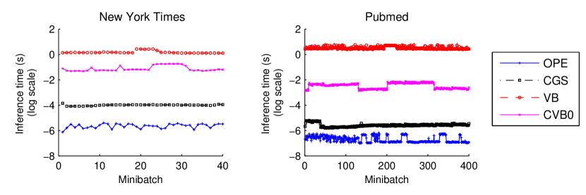
Figure 4: Average time to do inference for a doccument as the number of minibatches increases. Lower is faster. Note that OPE often performs many times faster than CGS, and hundreds times faster than VB.

Next we investigate the speed of inference. We took VB, CVB0, CGS, and OPE into consideration. For all of these methods, we compute the average time to do inference for a document at every minibatch when learning LDA. Figure 4 depicts the results. We find that among 4 inference methods, OPE consumed a modest amount of time, while CGS needed slightly more time. VB needed intensive time to do inference. The main reasons are that it requires various evaluations of expensive functions (e.g., log, exp, digamma), and that it needs to check convergence, which in our observation was often very expensive. Due to maintainance/update of many statistics which associate with each token in a document (see Table 1), CVB0 also consumed significant time. Note further that VB and CVB0 do not have any guarantee of convergence rate. Hence in practice VB and CVB0 might converge slowly.

Figure 4 suggests that OPE can perform fastest, compared with existing inference methods. Our investigation in the previous subsection demonstrates that OPE can find very good solutions for the posterior estimation problem. Those observations suggests that OPE is a good candidate for posterior inference in various situations.

5.3 Convergence and stability of OPE in practice

Our last investigation is about whether or not OPE performs stably in practice. We have to consider this behavior as there are two probabilistic steps in OPE: initialization of $\boldsymbol{\theta_{1}}$ and pick of $f_{t}$. To see stability, we took 100 testing documents from New York Times to do inference given the 100-topic LDA model previously learned by ML-OPE. For each document, we did 10 random runs for OPE, saved the objective values of the last iterates, and then computed the standard deviation of the objective values.

Stability of OPE is assessed via the standard deviation of the objective values. The smaller, the more stable. Figure 5 shows the histogram of the standard deviations computed from 100 functions. Each $T$ corresponds to a choice of the number of iterations for OPE.

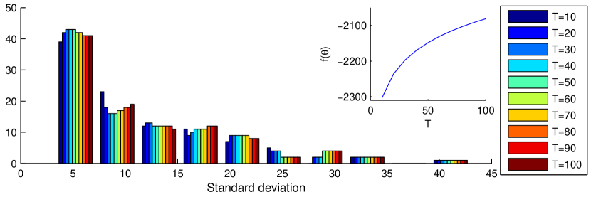
Figure 5: Convergence and stability of OPE in practice. The top-right corner shows convergence of OPE as allowing more iterations. The stability of OPE is measured by the standard deviation of the objective values ($f(\boldsymbol{\theta})$) from 10 random runs. The histogram (bar) for each setting of the number $T$ of iterations is computed from 100 different functions. This experiment was done on 100 documents of New York Times.

Observing Figure 5, we find that the standard deviation is small ($\leq 20$) for a large amount of functions. Comparing with the mean value of $f(\boldsymbol{\theta})$ which often belonged to $[-2300,-2000]$, the deviation is very small in magnitude. This suggests that for each function, the objective values returned by OPE from 10 runs seem not to significantly differ from each other. In other words, OPE behaved very stable in our observation.

Figure 5 also suggests that OPE converges very fast. The growth of $f(\boldsymbol{\theta})$ seems to be close to a linear function. This agrees well with Theorem 2 on convergence rate of OPE.

6 Conclusion

We have discussed how posterior inference for individual texts in topic models can be done efficiently. Our novel algorithm (OPE) is the first one which has a theorerical guarantee on quality and fast convergence rate. In practice, OPE can do inference very fast, and can be easily extended to a wide range of contexts including MAP estimation and non-convex optimization. By exploiting OPE carefully, we have arrived at new efficient methods for learning LDA from data streams or large corpora: ML-OPE, Online-OPE, and Streaming-OPE. Among those, ML-OPE and Online-OPE can reach state-of-the-art performance at a high speed. Furthermore, Online-OPE surpasses all existing methods in terms of predictiveness, and works well with short text. As a result, they are good candidates to help us deal with text streams and big data. The code of those methods are available at http://github.com/Khoat/OPE/.

Acknowledgments

This research is funded by Vietnam National Foundation for Science and Technology Development (NAFOSTED) under Grant Number 102.05-2014.28 and by the Air Force Office of Scientific Research (AFOSR), Asian Office of Aerospace Research & Development (AOARD), and US Army International Technology Center, Pacific (ITC-PAC) under Award Number FA2386-15-1-4011.

A Predictive Probability

Predictive Probability shows the predictiveness and generalization of a model $\mathcal{M}$ on new data. We followed the procedure in (Hoffman et al., 2013) to compute this quantity. For each document in a testing dataset, we divided randomly into two disjoint parts $\boldsymbol{w}_{obs}$ and $\boldsymbol{w}_{ho}$ with a ratio of 70:30. We next did inference for $\boldsymbol{w}_{obs}$ to get an estimate of $\mathbb{E}(\boldsymbol{\theta}^{obs})$. Then we approximated the predictive probability as

$$\Pr(\boldsymbol{w}_{ho}|\boldsymbol{w}_{obs},\mathcal{M})\approx\prod_{w\in\boldsymbol{w}_{ho}}\sum_{k=1}^{K}\mathbb{E}(\boldsymbol{\theta}^{obs}_{k})\mathbb{E}(\boldsymbol{\beta}_{kw}),$$

$$\text{Log Predictive Probability}=\frac{\log\Pr(\boldsymbol{w}_{ho}|\boldsymbol{w}_{obs},\mathcal{M})}{|\boldsymbol{w}_{ho}|},$$

where $\mathcal{M}$ is the model to be measured. We estimated $\mathbb{E}(\boldsymbol{\beta}_{k})\propto\boldsymbol{\lambda}_{k}$ for the learning methods which maintain a variational distribution ($\boldsymbol{\lambda}$) over topics. Log Predictive Probability was averaged from 5 random splits, each was on 1000 documents.

B NPMI

NPMI (Aletras and Stevenson, 2013; Bouma, 2009) is the measure to help us see the coherence or semantic quality of individual topics. According to Lau et al. (2014), NPMI agrees well with human evaluation on interpretability of topic models. For each topic $t$, we take the set $\{w_{1},w_{2},...,w_{n}\}$ of top $n$ terms with highest probabilities. We then computed

$$NPMI(t)=\frac{2}{n(n-1)}\sum_{j=2}^{n}\sum_{i=1}^{j-1}\frac{\log\frac{P(w_{j},w_{i})}{P(w_{j})P(w_{i})}}{-\log P(w_{j},w_{i})},$$

where $P(w_{i},w_{j})$ is the probability that terms $w_{i}$ and $w_{j}$ appear together in a document. We estimated those probabilities from the training data. In our experiments, we chose top $n=10$ terms for each topic.

Overall, NPMI of a model with $K$ topics is averaged as:

$$NPMI=\frac{1}{K}\sum_{t=1}^{K}NPMI(t).$$

References

- Aletras and Stevenson (2013) Nikolaos Aletras and Mark Stevenson. Evaluating topic coherence using distributional semantics. In Proceedings of the 10th International Conference on Computational Semantics, pages 13–22, 2013.
- Arora et al. (2016) Sanjeev Arora, Rong Ge, Frederic Koehler, Tengyu Ma, and Ankur Moitra. Provable algorithms for inference in topic models. In ICML, Journal of Machine Learning Research: W&CP, 2016.
- Asuncion et al. (2009) A. Asuncion, M. Welling, P. Smyth, and Y.W. Teh. On smoothing and inference for topic models. In Proceedings of the Twenty-Fifth Conference on Uncertainty in Artificial Intelligence, pages 27–34, 2009.
- Blei (2012) David M Blei. Probabilistic topic models. Communications of the ACM, 55(4):77–84, 2012.
- Blei et al. (2003) David M. Blei, Andrew Y. Ng, and Michael I. Jordan. Latent dirichlet allocation. Journal of Machine Learning Research, 3(3):993–1022, 2003.
- Bottou (1998) Léon Bottou. Online learning in neural networks. chapter Online Learning and Stochastic Approximations, pages 9–42. Cambridge University Press, 1998.
- Bouma (2009) Gerlof Bouma. Normalized (pointwise) mutual information in collocation extraction. Proceedings of GSCL, pages 31–40, 2009.
- Broderick et al. (2013) Tamara Broderick, Nicholas Boyd, Andre Wibisono, Ashia C Wilson, and Michael Jordan. Streaming variational bayes. In Advances in Neural Information Processing Systems, pages 1727–1735, 2013.
- Clarkson (2010) Kenneth L. Clarkson. Coresets, sparse greedy approximation, and the frank-wolfe algorithm. ACM Trans. Algorithms, 6:63:1–63:30, 2010. ISSN 1549-6325. doi: http://doi.acm.org/10.1145/1824777.1824783. URL http://doi.acm.org/10.1145/1824777.1824783.
- Dai et al. (2016) Bo Dai, Niao He, Hanjun Dai, and Le Song. Provable bayesian inference via particle mirror descent. In Proceedings of the 19th International Conference on Artificial Intelligence and Statistics, pages 985–994, 2016.
- Foulds et al. (2013) James Foulds, Levi Boyles, Christopher DuBois, Padhraic Smyth, and Max Welling. Stochastic collapsed variational bayesian inference for latent dirichlet allocation. In Proceedings of the 19th ACM SIGKDD International Conference on Knowledge Discovery and Data Mining, pages 446–454. ACM, 2013.
- Gao et al. (2015) Yang Gao, Zhenlong Sun, Yi Wang, Xiaosheng Liu, Jianfeng Yan, and Jia Zeng. A comparative study on parallel lda algorithms in mapreduce framework. In Advances in Knowledge Discovery and Data Mining, volume 9078 of LNCS, pages 675–689. Springer, 2015.
- Gerrish and Blei (2012) Sean Gerrish and David Blei. How they vote: Issue-adjusted models of legislative behavior. In Advances in Neural Information Processing Systems, volume 25, pages 2762–2770, 2012.
- Ghadimi and Lan (2013) Saeed Ghadimi and Guanghui Lan. Stochastic first-and zeroth-order methods for nonconvex stochastic programming. SIAM Journal on Optimization, 23(4):2341–2368, 2013.
- Griffiths and Steyvers (2004) T.L. Griffiths and M. Steyvers. Finding scientific topics. Proceedings of the National Academy of Sciences of the United States of America, 101(Suppl 1):5228, 2004.
- Grimmer (2010) Justin Grimmer. A bayesian hierarchical topic model for political texts: Measuring expressed agendas in senate press releases. Political Analysis, 18(1):1–35, 2010. doi: 10.1093/pan/mpp034. URL http://pan.oxfordjournals.org/content/18/1/1.abstract.
- Hazan and Kale (2012) Elad Hazan and Satyen Kale. Projection-free online learning. In Proceedings of the 29th Annual International Conference on Machine Learning (ICML), 2012.
- Hoffman et al. (2013) Matthew D Hoffman, David M Blei, Chong Wang, and John Paisley. Stochastic variational inference. The Journal of Machine Learning Research, 14(1):1303–1347, 2013.
- Lau et al. (2014) Jey Han Lau, David Newman, and Timothy Baldwin. Machine reading tea leaves: Automatically evaluating topic coherence and topic model quality. In Proceedings of the Association for Computational Linguistics, pages 530–539, 2014.
- Liu et al. (2010) B. Liu, L. Liu, A. Tsykin, G.J. Goodall, J.E. Green, M. Zhu, C.H. Kim, and J. Li. Identifying functional mirna–mrna regulatory modules with correspondence latent dirichlet allocation. Bioinformatics, 26(24):3105, 2010.
- Mai et al. (2016) Khai Mai, Sang Mai, Anh Nguyen, Ngo Van Linh, and Khoat Than. Enabling hierarchical dirichlet processes to work better for short texts at large scale. In Advances in Knowledge Discovery and Data Mining, volume 9652 of LNCS, pages 431–442. 2016.
- Mairal (2013) Julien Mairal. Stochastic majorization-minimization algorithms for large-scale optimization. In Advances in Neural Information Processing Systems, pages 2283–2291, 2013.
- McInerney et al. (2015) James McInerney, Rajesh Ranganath, and David Blei. The population posterior and bayesian modeling on streams. In Advances in Neural Information Processing Systems, pages 1153–1161, 2015.
- Mimno (2012) David Mimno. Computational historiography: Data mining in a century of classics journals. Journal on Computing and Cultural Heritage, 5(1):3, 2012.
- Mimno et al. (2012) David Mimno, Matthew D. Hoffman, and David M. Blei. Sparse stochastic inference for latent dirichlet allocation. In Proceedings of the 29th Annual International Conference on Machine Learning, 2012.
- Patterson and Teh (2013) Sam Patterson and Yee Whye Teh. Stochastic gradient riemannian langevin dynamics on the probability simplex. In Advances in Neural Information Processing Systems, pages 3102–3110, 2013.
- Pritchard et al. (2000) Jonathan K Pritchard, Matthew Stephens, and Peter Donnelly. Inference of population structure using multilocus genotype data. Genetics, 155(2):945–959, 2000.
- Sato and Nakagawa (2015) Issei Sato and Hiroshi Nakagawa. Stochastic divergence minimization for online collapsed variational bayes zero inference of latent dirichlet allocation. In Proceedings of the 21th ACM SIGKDD International Conference on Knowledge Discovery and Data Mining, pages 1035–1044. ACM, 2015.
- Schwartz et al. (2013) H Andrew Schwartz, Johannes C Eichstaedt, Lukasz Dziurzynski, Margaret L Kern, Martin EP Seligman, Lyle H Ungar, Eduardo Blanco, Michal Kosinski, and David Stillwell. Toward personality insights from language exploration in social media. In AAAI Spring Symposium Series, 2013.
- Simsekli et al. (2016) Umut Simsekli, Roland Badeau, Gaël Richard, and Taylan Cemgil. Stochastic quasi-newton langevin monte carlo. In Proceedings of the 33th International Conference on Machine Learning (ICML), 2016.
- Sontag and Roy (2011) David Sontag and Daniel M. Roy. Complexity of inference in latent dirichlet allocation. In Advances in Neural Information Processing Systems (NIPS), 2011.
- Tang et al. (2014) Jian Tang, Zhaoshi Meng, Xuanlong Nguyen, Qiaozhu Mei, and Ming Zhang. Understanding the limiting factors of topic modeling via posterior contraction analysis. In Proceedings of The 31st International Conference on Machine Learning, pages 190–198, 2014.
- Teh et al. (2016) Yee Whye Teh, Alexandre H Thiery, and Sebastian J Vollmer. Consistency and fluctuations for stochastic gradient langevin dynamics. Journal of Machine Learning Research, 17(7):1–33, 2016.
- Teh et al. (2007) Y.W. Teh, D. Newman, and M. Welling. A collapsed variational bayesian inference algorithm for latent dirichlet allocation. In Advances in Neural Information Processing Systems, volume 19, page 1353, 2007.
- Than and Doan (2014) Khoat Than and Tung Doan. Dual online inference for latent dirichlet allocation. In Proceedings of the 6th Asian Conference on Machine Learning (ACML), volume 39 of Journal of Machine Learning Research: W&CP, pages 80–95, 2014.
- Than and Ho (2015) Khoat Than and Tu Bao Ho. Inference in topic models: sparsity and trade-off. arXiv preprint arXiv:1512.03300, 2015. URL http://arxiv.org/abs/1512.03300.
- Than and Ho (2012) Khoat Than and Tu Bao Ho. Fully sparse topic models. In Peter Flach, Tijl De Bie, and Nello Cristianini, editors, Machine Learning and Knowledge Discovery in Databases, volume 7523 of Lecture Notes in Computer Science, pages 490–505. Springer, 2012.
- Yuille and Rangarajan (2003) Alan L Yuille and Anand Rangarajan. The concave-convex procedure. Neural computation, 15(4):915–936, 2003.